Gluon radiation by heavy quarks at intermediate energies

Abstract

Employing scalar QCD we study the gluon emission of heavy quarks created by the interaction with light quarks considered as dynamical scattering centers. We develop approximation formulas for the high energy limit and study when the full calculation reaches this high energy limit. For zero quark masses and in the high energy limit our model reproduces the Gunion-Bertsch results. We justify why scalar QCD represents a good approximation to the full QCD approach for the energy loss of heavy quarks. In the regime of accessible phenomenology we observe that the emission at small transverse momentum (dead cone effect) is less suppressed than originally suggested. We also investigate the influence of a finite gluon mass on the discussed results.

I Introduction

Lattice Gauge Theory predicts that at high temperatures/densities a new state of matter is formed, a plasma of quarks and gluons (QGP) Borsanyi:2010cj . There is strong circumstantial evidence that in ultrarelativistic heavy-ion collisions such a plasma is created for a short amount of time. It quickly expands and hadronizes. It is the main objective of the present experiments at the ultrarelativistic heavy ion colliders to study the properties of the QGP. The experiments of the last ten years at RHIC as well as the first runs at LHC have revealed that the hadron multiplicities are compatible with the assumption that hadrons are produced in statistical equilibrium at a temperature compatible with the predictions of Lattice Gauge calculations for the chiral/confinement phase transition Borsanyi:2010cj . Therefore the hadrons which are formed from plasma constituents are only of very limited use for the understanding of properties of the QGP.

For the study of the properties of the QGP during its expansion one has to rely on probes which do not come to an equilibrium with the plasma constituents. High-momentum heavy hadrons, those which contain a charm or a bottom quark, are such a probe. Due to the high energy required for their production heavy quarks are created in hard collisions during the initial phase of the reaction and do not annihilate in later phases Andronic:2007 . The number of these collisions can be determined from the collision geometry and the initial momentum distribution of the heavy quarks can be calculated from perturbative QCD (pQCD) Vogt:2003 ; Cacciari:2005 ; Cacciari:2012 . During the expansion of the plasma the heavy quarks interact with the plasma constituents, light quarks and gluons, but their initial momentum distribution is so different from that of the plasma particles that they do not come to thermal equilibrium Phenix:2011 ; ALICE:2012 . Therefore, their final momentum distribution at hadronization contains the desired information on the properties of the plasma during its evolution and this information is transferred to the heavy hadrons whose kinematics is largely determined by that of the entrained heavy quark.

The interpretation of the experimental (open) heavy flavor results is in reality a double challenge: One has to understand the elementary interaction of the heavy quarks with the plasma constituents but also the expansion of the plasma itself. For the same elementary interaction different expansion scenarios yield different results of the observables Gossiaux:2011ea .

Heavy quarks interact with the plasma constituents either by elastic collisions Bjorken ; Braaten:1991jj ; Peshier:2006hi ; Peigne:2008nd ; Gossiaux:2008jv or by inelastic radiative collisions Gyulassy94 ; Wang95 ; Baier95 ; Baier97 ; Zakharov ; GLV ; Dokshitzer:2001zm ; AMY ; Zakharov:2004 ; ASW ; Zhang:2004 ; Djordjevic:2004 or both Wicks:2007am . Whereas radiative collisions dominate the energy loss of light quarks, for the heavy quarks the relative importance of the elastic and of the radiative energy loss is debated. Detailed calculations for an expanding plasma are not available yet and the approximate calculations, using a static plasma of a given length, indicate that both are of the same order of magnitude  Wicks:2007am . Another complication for the judgement of the importance of the radiative energy loss is the Landau Pomeranchuck Migdal (LPM) effect, which states that radiative collisions are not independent but that a second gluon can only be emitted after the first one is formed.

For energetic light quarks the LPM effect in an infinite medium with a constant temperature and with static scattering centers has been evaluated independently by Zakharov Zakharov and by Baier, Dokshitzer, Mueller, Peigné and Schiff Baier95 ; Baier97 . Later it has been found that both approaches are identical Baier:2000mf and the approach has been extended to an expanding medium by applying time-dependent transport coefficients Baier:1998yf or time-dependent parton densities Zakharov:98 . More recently Arnold, Moore and Yaffe Arnold:2002ja , using diagrammatic methods, extended these calculations to dynamical gauge fields. The influence of the LPM effect for heavy quarks in a static medium is, however, presently still under debate and the calculation of how it shows up in an expanding medium whose temperature is rapidly changing is a theoretical challenge which has not been met yet.

A while ago we have advanced a pQCD-inspired calculation for the elastic collisions of heavy quarks with the QGP constituents which employs a running coupling constant and an infrared regulator which reproduces the energy loss of the heavy quarks in the hard thermal loop approach Gossiaux:2008jv ; Gossiaux:2009mk . Embedding these cross sections in the hydrodynamical description of the expanding plasma of Heinz and Kolb Kolb:2003dz we could show that the collisional energy loss underpredicts the measured energy loss of heavy mesons at large momenta as well as their elliptic flow by roughly a factor of two.

It is the purpose of this article to provide the basis for an extension of our pQCD calculation toward the calculation of the radiative energy loss. Some preliminary considerations have been published in Gossiaux:2010yx , where the calculation of Gunion:1981qs for the radiative cross section was extended to the case of a collision implying one heavy quark. In Gossiaux:2010yx , it is argued that for heavy quarks of intermediate energy, those which constitute the bulk of the production at RHIC and LHC, the gluon formation-time is strongly reduced by mass effects, so that coherence effects can be discarded in first approximation. In this respect, we offer a complementary viewpoint to the works of Dokshitzer:2001zm ; ASW ; Zhang:2004 ; Djordjevic:2004 ; Zakharov:2004 where heavy quarks are assumed to be ultrarelativistic and where the phase space boundaries are not of primary importance. The same viewpoint will be adopted in the present work in order to deduce and study the radiative cross section that will be later implemented in our Monte Carlo simulations in the same spirit as Fochler:2013 . The colliding light partons will be naturally considered as genuine dynamical degrees of freedom – see Djordjevic:2007at as well – and not as fixed scattering centers, as it was the case in most of the aforementioned works.

Starting out in section II from the standard QCD radiation matrix elements we calculate the gluon emission cross section for the collisions of a heavy quark with a light quark. The complexity of this result can be substantially reduced by realizing that matrix elements can be regrouped into three gauge invariant subgroups out of which one is dominating the energy loss. We then establish that pQCD and scalar QCD (SQCD) give only slightly different results as far as the energy loss of the heavy quark in a single collision is concerned. Therefore we continue our calculation in the SQCD approach which allows to compare our results with previous work of Gunion and Bertsch for the light quark sector Gunion:1981qs . We then discuss in section III the radiated gluon distribution and in particular the “dead cone” effect, the suppression of almost collinear gluon emission. This effect has been proposed a while ago by Dokshitzer and Kharzeev Dokshitzer:2001zm . We show that the emission of gluons with a small traverse momentum (with respect to the direction of the incoming quark) is reduced but remains finite as soon as this effect is calculated with gauge invariant matrix elements. In section IV we calculate the fractional radiative energy loss cross section $x\frac{d\sigma}{dx}$ as well as its integral over $x$ entering the calculation of the radiative energy loss $\frac{dE}{dz}$; we pay a particular attention to the kinematic region for which $s-M^{2}\gg T^{2}$ but $s$ not $\gg M^{2}$, relevant for production of heavy quarks at intermediate $p_{t}$ in ultrarelativistic heavy ion collisions at RHIC and LHC. In section V we extend the model by introducing a finite gluon mass, as done in a number of phenomenological approaches to study heavy ion collisions. We study in detail the influence of such a mass for the radiative energy loss. In section VI, we then provide a comparison of radiative and collisional energy loss. In an upcoming publication we will embed these results into a numerical simulation of the radiative and collisional energy loss using the hydrodynamical expansion scenario of ref. Werner:2010aa ; Werner:2012xh . Preliminary results for this approach have been presented recently gosssiaux:qnp .

II Model

II.1 Matrix elements

The starting point of our calculation are those five QCD bremsstrahlung diagrams which are of the order of $g^{3}$ and describe the creation of a gluon of 4-momentum $k$ in a collision between a heavy quark $Q$ with mass $M$ and incoming (outgoing) 4-momentum $P$ ($P^{\prime}$) and a light quark $q$ taken as massless with incoming (outgoing) 4-momentum $q$ ($q^{\prime}$) which is part of the plasma. They are shown in Fig. 1. $\ell=q-q^{\prime}$ is the 4-momentum transferred from the light quark. The matrix elements are given in Appendix A for completeness. We found that the quark spin is inessential. Considering scalar quarks is then sufficient and we give here $\mathcal{M}_{1}$, $\mathcal{M}_{2}$ and $\mathcal{M}_{3}$ in scalar QCD (SQCD, whose Feynman rules can be found in IZ ; Meggiolaro:1995cu )

$$\mathcal{M}_{1} = C_{1}\tilde{\mathcal{M}}_{1}=g^{3}C_{1}\ \frac{(q+q^{\prime})^{\mu}}{(q^{\prime}-q)^{2}}D_{\mu\nu}[q^{\prime}-q]\left\{\frac{(P-k+P^{\prime})^{\nu}(2P-k)\cdot\epsilon}{(P-k)^{2}-M^{2}}-\epsilon^{\nu}\right\},$$

$$\mathcal{M}_{2} = C_{2}\tilde{\mathcal{M}}_{2}=g^{3}C_{2}\ \frac{(q+q^{\prime})^{\mu}}{(q^{\prime}-q)^{2}}D_{\mu\nu}[q^{\prime}-q]\left\{\frac{(P+P^{\prime}+k)^{\nu}(2P^{\prime}+k)\cdot\epsilon}{(P^{\prime}+k)^{2}-M^{2}}-\epsilon^{\nu}\right\},$$

$$\mathcal{M}_{3} = C_{3}\tilde{\mathcal{M}}_{3}=g^{3}C_{3}\frac{(q+q^{\prime})^{\mu}(P+P^{\prime})^{\nu}}{(q^{\prime}-q)^{2}(P^{\prime}-P)^{2}}\,D_{\mu\mu^{\prime}}[q^{\prime}-q]D_{\nu\nu^{\prime}}[P^{\prime}-P]$$ (1)

$$\times \left\{g^{\mu^{\prime}\nu^{\prime}}(P-P^{\prime}+q^{\prime}-q)^{\sigma}+g^{\nu^{\prime}\sigma}(P^{\prime}-P-k)^{\mu^{\prime}}+g^{\sigma\mu^{\prime}}(q-q^{\prime}+k)^{\nu^{\prime}}\right\}\epsilon_{\sigma}\,.$$

In $\mathcal{M}_{1}$ and $\mathcal{M}_{2}$ the $\epsilon^{\nu}$-term comes from the extra diagram in SQCD where the emitted gluon is attached to the upper quark-exchanged-gluon vertex. We work in light cone gauge, $A\cdot n=0$ with $n$ being a fixed light-like vector, for which we find $D_{\mu\nu}[\ell]=-g_{\mu\nu}+\frac{\ell_{\mu}n_{\nu}+\ell_{\nu}n_{\mu}}{\ell\cdot n}$. The color matrix elements are

$$C_{1}=(T^{b}T^{a})(T^{b}),\quad C_{2}=(T^{a}T^{b})(T^{b}),\quad C_{3}=if_{abc}(T^{c})(T^{b}),$$ (2)

where the color matrix in the first (second) bracket is that of the heavy (light) quark. The two remaining matrix elements $\mathcal{M}_{4}$ and $\mathcal{M}_{5}$ can be obtained from $\mathcal{M}_{1}$ and $\mathcal{M}_{2}$ by exchanging heavy and light quark momenta ($P\leftrightarrow q$, $P^{\prime}\leftrightarrow q^{\prime}$) and color labels.

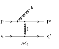
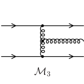
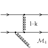
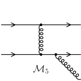
Figure 1: (Color online) The five matrix elements which contribute to the gluon bremsstrahlung in a collision between a heavy quark of incoming 4-momentum $P$ and a light quark of incoming 4-momentum $q$.

The commutation relation

$$T^{b}T^{a}=T^{a}T^{b}-if_{abc}T^{c},$$ (3)

allows for regrouping the five matrix elements into three combinations, each of them being gauge invariant:

$$\mathcal{M}^{\rm SQED}_{Q} = C_{2}(\tilde{\mathcal{M}}_{1}+\tilde{\mathcal{M}}_{2}),$$

$$\mathcal{M}^{\rm SQED}_{q} = C_{5}(\tilde{\mathcal{M}}_{4}+\tilde{\mathcal{M}}_{5}),$$

$$\mathcal{M}^{\rm SQCD} = C_{3}(\tilde{\mathcal{M}}_{3}-\tilde{\mathcal{M}}_{1}+\tilde{\mathcal{M}}_{4}),$$ (4)

where the $\tilde{\mathcal{M}}_{i}$ are defined in eq. 1. $Q$ ($q$) marks the emission of the gluon from the heavy (light) quark line. $C_{5}$ is obtained from $C_{2}$ by exchanging the heavy quark and light quark in eq. 2. The combination of diagrams labeled as SQED are the bremsstrahlung matrix elements already present in scalar Quantum Electrodynamics (SQED) whereas the amplitude labeled SQCD is a genuine matrix element of Quantum Chromo Dynamics. $\mathcal{M}^{\rm SQCD}$ is the main objet of interest here. It dominates the energy loss of heavy quarks, as we will show. In passing we mention that the decomposition of the five amplitudes into gauge invariant subgroups of diagrams is not unique. Beside the decomposition shown in eq. II.1 one can find a decomposition into commuting and anticommuting color operators. Such a decomposition has the advantage that the interference term disappears but the inconvenience of lengthy expressions.

II.2 Differential cross section at finite energy (model I)

It is convenient to specify the kinematics using a Sudakov decomposition of momenta. Pick $q$ as a light-like momentum (here chosen as the 4-momentum of the massless light quark) and choose $p$ such that $p^{2}=0$ and $P=p+b\,q$. From $P^{2}=M^{2}$ and $s=(P+q)^{2}$, it follows that

$$P=p+\frac{M^{2}}{2\,p\cdot q}q,\quad s=M^{2}+2\,p\cdot q.$$ (5)

The emitted gluon 4-momentum thus reads as

$$k=x\,p+k_{q}\,q+k_{t},\quad\mathrm{with}\quad k_{q}=\frac{\vec{k}_{t}^{2}}{2xp\cdot q}.$$ (6)

In this form, it is clear that the momentum fraction $x$ is a Lorentz invariant ($x=k\cdot q/p\cdot q$) and that $k_{t}$ is a space-like 4-vector which is transverse to both $p$ and $q$. Thus, it is equivalent to $\vec{k}_{t}\in\mathbb{R}^{2}$, with a norm $k_{t}^{2}=-\vec{k}_{t}^{2}$. Writing $\ell=\ell_{p}\,p+\ell_{q}\,q+\ell_{t}$, the set of independent variables can be chosen as $s$, $x$, the magnitude of $\vec{k}_{t}$, that of $\vec{\ell}_{t}$ and $\vec{k}_{t}\cdot\vec{\ell}_{t}$, or the angle $\phi_{k_{t}}$ between $\vec{k}_{t}$ and $\vec{\ell}_{t}$. $\mathcal{M}^{\rm SQCD}$ then reads as follows:

$$\mathcal{M}^{\rm SQCD}=g\,C_{3}\,\left(\frac{-4\,g^{2}\,P\cdot q}{\ell^{2}}\right)\left(\frac{(2(1-x)-x^{\prime})\,\vec{\epsilon}_{t}\cdot\vec{k}_{t}}{\vec{k}_{t}^{2}+x^{2}M^{2}}-\frac{2(1-x-x^{\prime})\,\vec{\epsilon}_{t}\cdot(\vec{k}_{t}-\vec{\ell}_{t})}{(\vec{k}_{t}-\vec{\ell}_{t})^{2}+(x+x^{\prime})^{2}M^{2}}\right).$$ (7)

In order to keep the matrix element in a compact form, the extra variable $x^{\prime}\equiv-\ell_{p}=-\ell^{2}/(2p\cdot q)$ is used in addition to the set of independent kinematical variables $(x,\vec{k}_{t},\vec{\ell}_{t})$. The appearance of $x^{\prime}$ and its deduction are explained in the Appendix B. Obtaining eq. 7 is straightforward, noticing that the occurrence of $x^{\prime}$ in the numerator partly comes from the identity $\frac{-2\,P\cdot q}{\ell^{2}}\times x^{\prime}=1$. The interest to factorize out $\frac{-2\,P\cdot q}{\ell^{2}}$ becomes clear at high energy as will be discussed shortly.

As it stands the matrix element is infrared sensitive. For a $qQ$ scattering taking place inside a QCD medium at finite temperature, the gluon propagator acquires finite electric and magnetic thermal masses Silva:2013 $m_{D}\sim gT$ and $m_{\rm mag}\sim g^{2}T$ which are usually interpreted in terms of screening effects. This screening prevents the cross section from being sensitive to $\sqrt{-\ell^{2}}$ smaller than the gluon mass, which acts therefore as a typical momentum transfer. The prescription for regularization that we adopt is to multiply the amplitude $\mathcal{M}$ by $\vec{\ell}_{t}^{2}/(\vec{\ell}_{t}^{2}+\mu^{2})$, with $\mu\sim gT$. There are other propositions, to use hard thermal loop calculations Braaten:1991jj ; Djordjevic:2007at or to introduce a self consistent temperature dependent Debye mass Peshier:2007 .

After squaring the matrix element, summing over the transverse polarizations, and making use of the phase space integral derived in Appendix B, one obtains, for the gluon emission cross section:

$$\frac{d\sigma^{Qq\rightarrow Qgq}}{dxd^{2}k_{t}d^{2}\ell_{t}}=\frac{1}{2(s-M^{2})}|\mathcal{M}|^{2}\frac{1}{4(2\pi)^{5}\,\sqrt{\Delta}}\Theta(\Delta)\,,$$ (8)

with

$$\Delta=\left(x(1-x)\,s-x\,M^{2}-\vec{k}_{t}^{2}+2x\,\vec{k}_{t}\cdot\vec{\ell}_{t}\right)^{2}-4x(1-x)\,\vec{\ell}_{t}^{2}\,(x\,s-\vec{k}_{t}^{2}).$$ (9)

The evaluation of $\frac{d\sigma^{Qq\rightarrow Qgq}}{dxd^{2}k_{t}d^{2}\ell_{t}}$, eq. 8, with $\mathcal{M}=\mathcal{M}^{\rm SQCD}$, eq. 7, gives what we call the finite energy cross section, model I. With the presence of $x^{\prime}$ and its somewhat complicated dependence on the other variables the full result does not allow for an easy physical discussion at all energies. In section IV.2 we present the numerical results in which the full matrix element, eq. 7, is used and the subsequent integration over the phase space variables has been done by a Monte Carlo method. This allows for taking into account the boundaries of the integration in a very convenient way.

The physics becomes more transparent when we go to the high energy limit where subleading terms in $\sqrt{s}$ are neglected. This limit has also the advantage that the expressions for the differential as well as for the various integrated cross sections become very compact. One of the aims of the present study is to investigate the accuracy of the high-energy approximation with respect to the full result.

II.3 High-energy approximation and model II

To elucidate the physics of the gluon emission we specify the high-energy regime of interest. Assuming that $s\approx 2P\cdot q$, i.e., $M^{2}\ll s$, our discussion parallels that of Gunion and Bertsch Gunion:1981qs . At the end of the section we examine more deeply the interplay between $M^{2}$ and $s$ in order to specify what happens if $M^{2}\ll s$ is not fulfilled. However, this discussion is easier to carry out a posteriori.

At high energy there is room for radiation in a wide rapidity interval Gunion:1981qs . The central region, $x\ll 1$ and $k_{q}\equiv\frac{\vec{k}_{t}^{2}}{2xp\cdot q}\ll 1$, is driven by $\mathcal{M}^{\mathrm{SQCD}}$, which thus forms the bulk of radiation (see Gunion:1981qs and also the discussion in section III). $\mathcal{M}^{\mathrm{SQED}}_{Q}$ and $\mathcal{M}^{\mathrm{SQED}}_{q}$ become competitive respectively at large $x$ and at large $k_{q}$ (corresponding to very small $x$), but are otherwise suppressed. In section III, it is shown that the important region of phase space for radiation is $\vec{k}_{t}^{2}\lesssim|\ell^{2}|$. This is a consequence of the $1/(\vec{k}_{t}^{2})^{2}$ behavior of the differential cross section, eq. 8, with the matrix element, eq. 7, at large $\vec{k}_{t}^{2}$ for fixed $t\equiv\ell^{2}$. In addition the $1/t^{2}$ suppression of the differential cross section at large $|t|$ makes the large $|t|$ region essentially irrelevant.

We therefore define the large $s$ domain as

$$s,x\,s\gg|\ell^{2}|,\vec{k}_{t}^{2}.$$ (10)

It encompasses the rapidity interval between the fragmentation regions of heavy and light quarks where $x$ is small but not that small that it approaches the light quark fragmentation regime $x\sim\vec{k}_{t}^{2}/s$. The latter region will be discarded from the analysis. Eq. 10 also covers the heavy quark fragmentation region, where $x$ is finite, $x\sim 1$, allowing us to quantify the relative importance of $\mathcal{M}^{\mathrm{SQCD}}$ and $\mathcal{M}^{\mathrm{SQED}}_{Q}$, see Appendix C.

In leading order of $s$ all squares of the matrix elements, $|\mathcal{M}|^{2}$, factorize

$$|\mathcal{M}|^{2}=16\pi^{3}x(1-x)\,|\mathcal{M}_{\rm el}(s,\vec{\ell}_{t})|^{2}P_{g}(x,\vec{k}_{t},\vec{\ell}_{t}),$$ (11)

with $|\mathcal{M}_{\rm el}(s,\vec{\ell}_{t})|^{2}=\frac{C_{F}}{2N_{c}}g^{4}\frac{4s^{2}}{(\vec{\ell}_{t}^{2}+\mu^{2})^{2}}$ being the regularized matrix element squared for the elastic cross section at high energy ($C_{F}/(2N_{c})=2/9$). As a consequence the differential cross section can be written as

$$\frac{d\sigma^{Qq\rightarrow Qgq}}{dxd^{2}k_{t}d^{2}\ell_{t}}\underset{s\gg M^{2}}{\to}\frac{d\sigma_{\rm el}}{d^{2}\ell_{t}}\,P_{g}(x,\vec{k}_{t},\vec{\ell}_{t}),$$ (12)

with $\frac{d\sigma_{\rm el}}{d^{2}\ell_{t}}\rightarrow\frac{8\alpha_{s}^{2}}{9(\vec{\ell}_{t}^{2}+\mu^{2})^{2}}$. We mention that the spin averaged square of the QCD matrix element is the sum of $|\mathcal{M}^{\rm SQCD}|^{2}$ which is the squared matrix element for the same bremsstrahlung process in SQCD and a correction term which is negligible at small $x$, the dominating region of the gluon emission:

$$\frac{1}{4}\sum_{\rm spin}|\mathcal{M}^{\rm QCD}|^{2}=|\mathcal{M}^{\rm SQCD}|^{2}+\frac{x^{2}}{2(1-x)}\frac{\vec{\ell}_{t}^{2}}{(\vec{k}_{t}^{2}+x^{2}M^{2})\left((\vec{k}_{t}-\vec{\ell}_{t})^{2}+x^{2}M^{2}\right)}C_{A}16\pi\alpha_{s}(1-x)^{2}|\mathcal{M}_{\rm el}|^{2}.$$ (13)

The color factor is $C_{A}=3$. Thus at small $x$, as we will see, the dominant region for the energy loss as well as for the gluon emission, spinor QCD can be well approximated by scalar QCD and we can profit from the fact that $|\mathcal{M}^{\rm SQCD}|^{2}$ has in the large energy limit a very simple form:

$$|\mathcal{M}^{\rm SQCD}|^{2}=C_{A}16\pi\alpha_{s}(1-x)^{2}|\mathcal{M}_{\rm el}|^{2}\left(\frac{\vec{k}_{t}}{\vec{k}_{t}^{2}+x^{2}M^{2}}-\frac{\vec{k}_{t}-\vec{\ell}_{t}}{(\vec{k}_{t}-\vec{\ell}_{t})^{2}+x^{2}M^{2}}\right)^{2},$$ (14)

leading to

$$P_{g}(x,\vec{k}_{t},\vec{\ell}_{t};M)=\frac{C_{A}\alpha_{s}}{\pi^{2}}\frac{1-x}{x}\left(\frac{\vec{k}_{t}}{\vec{k}_{t}^{2}+x^{2}M^{2}}-\frac{\vec{k}_{t}-\vec{\ell}_{t}}{(\vec{k}_{t}-\vec{\ell}_{t})^{2}+x^{2}M^{2}}\right)^{2}.$$ (15)

In light-cone gauge with fixing gauge vector $n=q$, the first term in the bracket describes the emission from the incoming heavy quark line and the second term the emission from the gluon. This shows that in this gauge and away from the light quark fragmentation region the matrix element for the emission from the light quark does not contribute. In Sect. IV.2 the comparison between the full result, model I, and the high-energy approximation will allow for a quantitative judgement of the relevance of the latter in the phenomenologically accessible range of $\sqrt{s}$.

The high-energy approximation eq. 14 is easily obtained by setting $x^{\prime}\to 0$ in eq. 7 . Using this result in eq. 8 and approximating $\sqrt{\Delta}\approx x(1-x)\,s$, $s-M^{2}\approx s$ and $-t\approx\vec{\ell}_{t}^{2}$, but keeping the exact phase space boundaries eqs. 50, gives an approximation, referred to as model II, that incorporates part of the finite energy corrections easy to implement:

$$\frac{d\sigma^{Qq\rightarrow Qgq}_{II}}{dxd^{2}k_{t}d^{2}\ell_{t}}=\frac{d\sigma_{\rm el}}{d^{2}\ell_{t}}\,P_{g}(x,\vec{k}_{t},\vec{\ell}_{t})\Theta(\Delta)\,.$$ (16)

Model II is situated midway between the full calculation, model I, and the high-energy approximation eq. 12.

We observe that the high-energy approximation does not necessarily require $s$ to be much bigger than $M^{2}$ in $\mathcal{M}^{\rm SQCD}$. Only $x^{\prime}\ll x$ and $x^{\prime}\ll 1-x$ are mandatory. The first condition writes $-t\ll x(s-M^{2})$, which can be fulfilled for moderate $t$ even if $s$ is not very large with respect to $M^{2}$. In such a circumstance, one power of $2\,P\cdot q=s-M^{2}$ in $|\mathcal{M}^{\rm SQCD}|^{2}$ cancels out with the same factor in the denominator of eq. 8 while the second power cancels out exactly at small $x$ where $\sqrt{\Delta}\approx x\,(s-M^{2})$. Thus, imposing both $x^{\prime}\ll x$ and $k_{q}\ll 1$, corresponding to $\vec{k}_{t}^{2}\ll x\,(s-M^{2})$, eq. 10 is replaced by

$$s-M^{2},\ x\,(s-M^{2})\gg|\ell^{2}|,\vec{k}_{t}^{2}.$$ (17)

In the case of massless quarks, eq. 14 is identical with the matrix elements of Gunion and Bertsch (GB) of ref. Gunion:1981qs . Their discussion at the amplitude level is carried through within SQCD at both small $x$ and finite $x$. In spinor QCD, even for massless quarks, we were able to compute finite $x$ correction only at the squared amplitude level. At $M=0$, we observe the factorization between transverse ($\vec{k}_{t}$, $\vec{\ell}_{t}$) and longitudinal ($x$) dependence, and for the latter a factor $2(1-x)$ in SQCD and $2(1-x)+x^{2}$ in spinor QCD which is reminiscent of the quark splitting functions in SQCD and QCD.

Similarly we derive the QED-like terms. $|\mathcal{M}^{\rm QED}_{Q}|^{2}$ can be directly drawn from eqs 13 and 14 by changing $\vec{\ell}_{t}\to x\vec{\ell}_{t}$ and the color factor $C_{A}\to C_{F}=4/3$. At small $x$, one gets $|\mathcal{M}^{\rm QED}_{Q}|^{2}=|\mathcal{M}^{\rm SQED}_{Q}|^{2}+\mathcal{O}(x^{2})$ with

$$|\mathcal{M}^{\rm SQED}_{Q}|^{2}=C_{F}\ 16\pi\alpha_{s}(1-x)^{2}|\mathcal{M}_{\rm el}|^{2}\left(\frac{\vec{k}_{t}}{\vec{k}_{t}^{2}+x^{2}M^{2}}-\frac{\vec{k}_{t}-x\vec{\ell}_{t}}{(\vec{k}_{t}-x\vec{\ell}_{t})^{2}+x^{2}M^{2}}\right)^{2}.$$ (18)

III Gluon distribution in the high energy approximation

In this section, we study the gluon distribution $P_{g}$ as a function of $k_{t}$ (from now on, $k_{t}$ will refer to $|\vec{k}_{t}|$ and $\ell_{t}$ to $|\vec{l}_{t}|$). $P_{g}$ exhibits the well-known bremsstrahlung phenomenology. When $\ell_{t}$ and $xM$ are incommensurate, there are two extreme regimes: the hard scattering regime, $\ell_{t}\gg xM$, and the soft scattering regime, $\ell_{t}\ll xM$. Inspection of eq. 14 shows that the important region for radiation is that of intermediate $k_{t}$ since $P_{g}$ remains finite at small $k_{t}$ and $P_{g}\propto k_{t}^{-4}$ at large $k_{t}$. Thus, for a hard scattering we find

$$P_{g}\propto\frac{\vec{k}_{t}^{2}}{(\vec{k}_{t}^{2}+x^{2}M^{2})^{2}},$$ (19)

assuming $\frac{x^{2}M^{2}}{\ell_{t}}\ll k_{t}\ll\ell_{t}$. In the hard scattering regime, the radiation is logarithmically enhanced for $k_{t}\gg xM$ and there is a dead cone for $k_{t}<xM$. There the ratio between the gluon distribution function for the massive and massless cases reads

$$K_{\mathrm{HQ}}=\frac{P_{g}(x,\vec{k}_{t},\vec{\ell}_{t};M)}{P_{g}(x,\vec{k}_{t},\vec{\ell}_{t};0)}=\frac{1}{\left(1+\frac{x^{2}M^{2}}{\vec{k}_{t}^{2}}\right)^{2}}.$$ (20)

The situation of hard scatterings on the medium is implicitly assumed in the analysis of Ref. Dokshitzer:2001zm . For soft scattering, $\ell_{t}\ll xM$, there is a strong interference between both factors in the bracket of eq. 14 and no room for large (i.e. log-enhanced) radiation.

Considering charm or bottom quarks, $M=1.3$, 4.5 GeV, in a medium characterized by $\mu=0.4$ GeV, both regimes are encountered in the $x,\ell_{t}$ plane and we now study quantitatively the resulting $k_{t}$ dependence.

III.1 Integration over $\angle(\vec{\ell}_{t},\vec{k}_{t})$

In the high energy limit the integral over $\phi_{k_{t}}$ can be performed analytically over $[0,2\pi]$:

$$\mathcal{I}(x,k_{t},\ell_{t};M) = \int d\phi_{k_{t}}P_{g}(x,\vec{k}_{t},\vec{\ell}_{t})=\frac{2C_{A}\alpha_{s}}{\pi}\frac{1-x}{x}\left[\frac{\vec{\ell}_{t}^{2}+2x^{2}M^{2}}{\left(\vec{k}_{t}^{2}+x^{2}M^{2}\right)\left(\left(\vec{k}_{t}^{2}+x^{2}M^{2}+\vec{\ell}_{t}^{2}\right)^{2}-4\vec{k}_{t}^{2}\vec{\ell}_{t}^{2}\right)^{1/2}}\right.$$ (21)

$$\left.-\frac{x^{2}M^{2}}{(\vec{k}_{t}^{2}+x^{2}M^{2})^{2}}-\frac{x^{2}M^{2}(\vec{k}_{t}^{2}+x^{2}M^{2}+\vec{\ell}_{t}^{2})}{\left(\left(\vec{k}_{t}^{2}+x^{2}M^{2}+\vec{\ell}_{t}^{2}\right)^{2}-4\vec{k}_{t}^{2}\vec{\ell}_{t}^{2}\right)^{3/2}}\right],$$

and one finds for zero mass quarks as well the GB result:

$$\mathcal{I}(x,k_{t},\ell_{t};M=0)=\frac{2C_{A}\alpha_{s}}{\pi}\frac{1-x}{x}\frac{\vec{\ell}_{t}^{2}}{\vec{k}_{t}^{2}|\vec{k}_{t}^{2}-\vec{\ell}_{t}^{2}|}.$$ (22)

Again, the corresponding SQED term can be obtained by replacing $\vec{\ell}_{t}\to x\vec{\ell}_{t}$ and $C_{A}\to C_{F}$.

Fig. 2 shows the behaviour of $\mathcal{I}$ for $\ell_{t}=1$, $xM=0.01$ (dashed black line) and $\ell_{t}=0.01$, $xM=1$ (full red line), chosen to make visible the aforementioned hard and soft scattering regimes. In Fig. 2 $\mathcal{I}$ is divided by its value at $k_{t}=0$:

$$\mathcal{I}(x,0,\ell_{t};M)=\frac{2C_{A}\alpha_{s}}{\pi}\frac{1-x}{x}\frac{\vec{\ell}_{t}^{2}}{(\vec{\ell}_{t}^{2}+x^{2}M^{2})^{2}}.$$ (23)

For comparison, the “dead cone” distribution eq. 19 is also plotted for $xM=0.01$ (dash-dotted blue line).

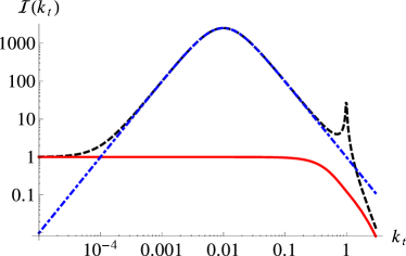
Figure 2: (Color online) $k_{t}$ distribution of gluons. The full red line and the dashed black line correspond to $\mathcal{I}(x,k_{t},t;M)$, eq. 21, with $\ell_{t}=0.01,xM=1$ and $\ell_{t}=1,xM=0.01$, respectively, while the dash-dotted blue line corresponds to the dead cone distribution, eq. 19, with $xM=0.01$.

We observe that for hard scattering $\mathcal{I}(x,|\vec{k}_{t}|,\ell_{t};M)$ falls off $\propto 1/|\vec{k}_{t}|^{4}$ for large $k_{t}$. This can be directly read off from eq. 14 setting $M=0$ which leads us back to the Gunion-Bertsch behavior, eq. 22. For $k_{t}$ in between $(xM)^{2}/\ell_{t}$ and $\ell_{t}$, $\mathcal{I}$ behaves as indicated in eq. 19, which corresponds to dropping the second term in the bracket of eq. 14, hence we observe the absence of interference in this range: on the plot, the dash-dotted line is on top of the dashed line. As anticipated, we observe a log-enhanced radiation $\mathcal{I}\propto 1/\vec{k}_{t}^{2}$ for $xM<k_{t}<\ell_{t}$ and a dead cone suppression for $(xM)^{2}/\ell_{t}<k_{t}<xM$, as well as a maximum at $k_{t}\sim xM$. The second region of enhanced radiation on Fig. 2, visible around $k_{t}=\ell_{t}$ , is due to the second term in the bracket of eq. 14.

For soft scattering, keeping only terms of at most $\mathcal{O}(\vec{\ell}_{t}^{2})$, we find

$$\mathcal{I}(x,k_{t},\ell_{t};M)=\frac{2C_{A}\alpha_{s}}{\pi}\frac{1-x}{x}\frac{\vec{\ell}_{t}^{2}}{(\vec{k}_{t}^{2}+x^{2}M^{2})^{2}}\times\frac{|\vec{k}_{t}|^{4}+x^{4}M^{4}}{(\vec{k}_{t}^{2}+x^{2}M^{2})^{2}}.$$ (24)

This behavior results from a strong interference between the two terms in the bracket of eq. 14, since both terms can be large but their difference is small in this regime. The full line shows the direct transition from a constant value at small $k_{t}$ to a $1/|\vec{k}_{t}|^{4}$ dependence for large $k_{t}$. This behavior is easily obtained from the approximation in eq. 24, noticing that the last factor is 1 in both limits.

III.2 Gluon emission in $x-k_{t}$ space and the dead cone effect

One step further can be made by averaging over the elastic cross section, defining

$${\bar{P}}_{g}(x,k_{t};M)=\frac{\int d^{2}\vec{\ell}_{t}\frac{1}{(\vec{\ell}_{t}^{2}+\mu^{2})^{2}}P_{g}(x,\vec{k}_{t},\vec{\ell}_{t})}{\int d^{2}\vec{\ell}_{t}\frac{1}{(\vec{\ell}_{t}^{2}+\mu^{2})^{2}}},$$ (25)

with an infrared regularization for the elastic cross section as discussed above. Let us notice that due to the fast decrease of the differential elastic cross section with $|\vec{l}_{t}|$, the gross features of ${\bar{P}}_{g}$ can be obtained from those of $P_{g}$ – or more precisely from those of ${\cal I}/(2\pi)$ in eq. 21 – by substituting $\mu$ for $|\vec{l}_{t}|$. Contours of the distribution of gluons emitted from a charm quark as a function of $x$ and $k_{t}$, ${\bar{P}}_{g}(x,k_{t};M)$, are shown in fig. 3(left). We have illustrated the case $\mu<M$ which includes both hard and soft scattering regimes. We see that the radiation is concentrated at small $x$ (in the hard scattering regime) and small $k_{t}$ - values.

Figure 3: Left: Contour plot of the $x$ and $k_{t}$ distribution of gluons emitted from charm quarks, $\bar{P}_{g}(x,k_{t};M=1.3~{}\mathrm{GeV})$, in logarithmic scale. Right: Contour plot of the relative contribution of the QED-like cross section to the total gluon emission cross section for $M=1.3~{}\mathrm{GeV}$ as a function of $x$ and $k_{t}$. The infrared regulator is chosen as $\mu=0.4$ GeV. The dashed line at $x=\mu/M$ indicates the transition from hard scattering regime ($x\lesssim\mu/M$) to soft scattering regime ($x\gtrsim\mu/M$).

The QED-like term, eq. 18, contributes only little to the overall radiation, as can be seen in Fig. 3(right) which shows contours of the ratio ${\bar{P}}_{g}^{\rm SQED}/{\bar{P}}_{g}^{tot}$ as a function of $x$ and $k_{t}$ for $M=1.3$ GeV. ${\bar{P}}_{g}^{tot}$ is built from $|\mathcal{M}^{\rm SQCD}+\mathcal{M}_{Q}^{\rm SQED}|^{2}$ whereas ${\bar{P}}_{g}^{\rm SQED}$ is built from $|\mathcal{M}_{Q}^{\rm SQED}|^{2}$.

In the regime of hard scattering, at small $x\lesssim\mu/M$, the QED-like contribution is marginal for almost all $k_{t}$. The ratio becomes sizable (property A) for very small $k_{t}$ only, $k_{t}<\frac{x^{2}M^{2}}{\langle l_{t}\rangle}\approx\frac{x^{2}M^{2}}{\mu}<xM$, corresponding to large rapidities Gunion:1981qs . The SQED contribution can even become the dominant one (property B) for $x<\mu^{2}/M^{2}$ and $k_{t}<x\langle l_{t}\rangle\approx x\mu<xM$. In both cases however, those regions of phase phase space are very limited in comparison to the range $k_{t}\in[xM,\mu]$ where the QCD radiation is large. The ratio becomes sizable (property C) also in the soft scattering regime (at large $x$), where the radiation is weak. A more detailed analysis is given in Appendix C. The second QED-like term, $|\mathcal{M}^{\rm SQED}_{q}|^{2}$, describing the gluon emission from the light quark, is irrelevant at high-energy away from the light-quark fragmentation region.

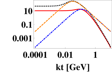
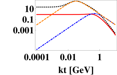
Figure 4: (Color online) The suppression of gluon radiation of quarks, $\bar{P}_{g}(x=0.1,k_{t},M)$, in our approach (red full line and black dotted line for the emission from a heavy quark and of a quark with mass $M=0.1$ GeV, respectively) as compared to the hard scattering approach, eq. 19, (blue dash-dotted line and orange dashed line for the emission from heavy and $M=0.1$ GeV quarks, respectively). On the left hand side we display the results for charm quarks, $M=1.3$ GeV, and on the right hand side for bottom quarks, $M=4.5$ GeV.

Fig. 4 compares our results, eq. 25, including the squared matrix element given by eq. 14, with the dead cone approximation eq. 19. The red full line shows on the left (right) hand side the $k_{t}$ distribution of gluons at $x=.1$, ${\bar{P}}_{g}(x=0.1,k_{t};M)$, emitted from charm (bottom) quarks, and the black dashed line shows the distribution of gluons emitted from light quarks with $M=0.1$ GeV. These curves are compared with the results of the hard scattering approach (blue dash-dotted line for the heavy quark and orange dashed line for the light quarks). The main features, discussed in the last section for a fixed $\ell_{t}$, are still visible after the averaging over elastic cross section, $\ell_{t}$ being replaced by $\mu$. For the light quark, and the chosen $x$-value, $xM$ is much smaller than $\mu$ and the characteristics of the hard scattering regime are visible. In particular, we observe a strong radiation window at intermediate $k_{t}\lesssim\mu$ that is fairly well reproduced by the dead cone approximation. For the bottom quark, for which $xM$ is comparable to $\mu$, the trend is typical of the soft scattering regime, with nowhere a match with the dead cone approximation.

The suppression of the radiation from heavy quarks as compared to that from light quarks at small $k_{t}$ can be quantified by a suppression factor $\bar{K}$

$$\bar{K}(x,k_{t};M)={\bar{P}}_{g}(x,k_{t};M)/{\bar{P}}_{g}(x,k_{t};M=0.1\ \mathrm{GeV}).$$ (26)

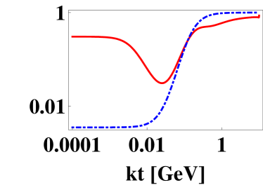
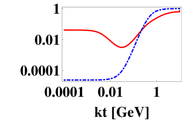
Figure 5: (Color online) The suppression of radiation (as compared to that from light quarks) at $x=0.1$ for charm quarks, left, and for bottom quarks, right. The full red line is the SQCD result, $\bar{K}$, and the dash-dotted blue line corresponds to the dead cone ratio $K_{\mathrm{HQ}}$, eq. 20.

In fig. 5 we display this suppression of radiation from a charm quark, left, and from a bottom quark, right, for $x=.1$ as a function of $k_{t}$. The full red line is the SQCD result, $\bar{K}(x=0.1,k_{t};M)$, and the dash-dotted blue line is the result of the hard scattering approach, for which $\bar{K}=K_{\mathrm{HQ}}$, see eq. 20. The suppression of the yield at small $k_{t}$ is largely overestimated in the latter approach, but, more important for the whole radiation, the SQCD ratio behaves as $\vec{k}_{t}^{2}$ at intermediate $k_{t}$ when $xM$ is comparable to $\mu$ (this is the case for the bottom quark in fig. 5) instead of the $(\vec{k}_{t}^{2})^{2}$ rise of $K_{\mathrm{HQ}}$. For somewhat smaller $xM$ (charm quark case in fig. 5), the rise after the dip is comparable to that of $K_{\mathrm{HQ}}$ in the middle of the range but there is an extra reduction visible for higher $k_{t}$. Looking at fig. 4, the latter effect corresponds to the depletion of the full curve relative to the dash-dotted curve. It is a consequence of the mass effect in the region where $k_{t}$ is comparable to $xM$. Such a feature is already present before $\ell_{t}$ averaging where it can be attributed to the departure from 1 of the last factor in eq. 24.

These results show that the mass effect on radiation is more involved than what can be modeled with a simple “dead cone suppression” factor. A similar conclusion was reached in Ref. ASW in a situation that goes beyond one single averaged scattering.

IV Radiation Cross Section and Power Spectrum

We now come back to the case of finite $s$ and perform successively the integration on $\vec{k}_{t}$ and $\vec{l}_{t}$ to obtain the differential cross section $\frac{d\sigma^{Qq\rightarrow Qgq}}{dx}$ which describes the power spectrum.

IV.1 Integration over $k_{t}$

For the “exact” model, model I, performing the integration over $k_{t}$ is rather involved and a numerical approach was preferred. In the case of model II, eq. 16, the simple integrand makes it possible to perform the integration over $k_{t}$ analytically provided one neglects the angular dependence of the phase space boundary, which is indeed rather mild under the conditions of eq. 17.:

$$\int\!P_{g}\,\Theta(K_{t}-k_{t})d^{2}\vec{k}_{t} = \frac{C_{A}\alpha_{s}}{\pi}\frac{1-x}{x}\left(-\frac{K_{t}^{2}}{K_{t}^{2}+x^{2}M^{2}}-\frac{1}{2}-\frac{K_{t}^{2}-\vec{\ell}_{t}^{2}-x^{2}M^{2}}{2\sqrt{K_{t}^{4}-2\left(\vec{\ell}_{t}^{2}-x^{2}M^{2}\right)K_{t}^{2}+\left(\vec{\ell}_{t}^{2}+x^{2}M^{2}\right)^{2}}}\right.$$

$$+ \frac{\vec{\ell}_{t}^{2}+2x^{2}M^{2}}{\sqrt{\vec{\ell}_{t}^{2}(\vec{\ell}_{t}^{2}+4x^{2}M^{2})}}\left[\log\frac{\vec{\ell}_{t}^{2}+3x^{2}M^{2}+\sqrt{1+4x^{2}M^{2}/\vec{\ell}_{t}^{2}}\;(\vec{\ell}_{t}^{2}+x^{2}M^{2})}{x^{2}M^{2}}\right.$$

$$- \left.\left.\log\frac{-K_{t}^{2}+\vec{\ell}_{t}^{2}+3x^{2}M^{2}+\sqrt{1+4x^{2}M^{2}/\vec{\ell}_{t}^{2}}\,\sqrt{K_{t}^{4}-2\left(\vec{\ell}_{t}^{2}-x^{2}M^{2}\right)K_{t}^{2}+\left(\vec{\ell}_{t}^{2}+x^{2}M^{2}\right)^{2}}}{K_{t}^{2}+x^{2}M^{2}}\right]\right)\,,$$

Physics-wise, the expression for the upper limit of the $k_{t}$ integration $K_{t}\rightarrow k_{\rm max}(s,\ell_{t})$ is given by the root of $\Delta$ in eq. 9. It is shown in fig. 6, as a function of $\ell_{t}$ (left) and as a function of $x$ (right). Except close to the boundaries, $x=0$ and $x=x_{\mathrm{max}}=(s-M^{2})/s$ the kinematically allowed values reach several GeV for typical $\ell_{t}$, $\ell_{t}=\mathcal{O}(\mu)\leq 1$ GeV. In this situation, the high energy limit $K_{t}\to\infty$ should provide a reasonable approximation of the full expression. Requiring $K_{t}\gg\mu$ at $x=x_{\mathrm{max}}/2$ translates into $s-M^{2}\gg 2\sqrt{s}\mu$. For realistic numbers, we anticipate a failure of the high-energy approximation in the whole $x$-range for $\sqrt{s}\leq 2$ GeV, respectively 5 GeV, in the case of a charm, respectively bottom, quark.

In the $K_{t}\to\infty$ limit, eq. IV.1 simplifies considerably:

$$\int P_{g}d^{2}\vec{k}_{t}=\frac{C_{A}\alpha_{s}}{\pi}\frac{1-x}{x}\left(\frac{\vec{\ell}_{t}^{2}+2x^{2}M^{2}}{\sqrt{\vec{\ell}_{t}^{2}(\vec{\ell}_{t}^{2}+4x^{2}M^{2})}}\log\left(\frac{\vec{\ell}_{t}^{2}\left(\sqrt{1+4x^{2}M^{2}/\vec{\ell}_{t}^{2}}+1\right)+4x^{2}M^{2}}{x^{2}M^{2}\left(\sqrt{1+4x^{2}M^{2}/\vec{\ell}_{t}^{2}}-1\right)}+1\right)-2\right).$$ (28)

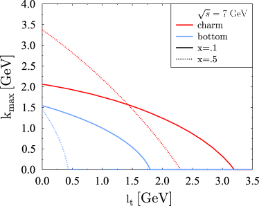
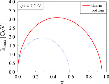
Figure 6: (Color online) The upper integration limit $k_{\mathrm{max}}$ as a function of $\ell_{t}$ for $x=.1$ and $x=.6$ and for charm and bottom quarks (left) and as a function of $x$ for $\ell_{t}=.3$ GeV for charm and bottom quarks (right).

In fig. 7 we show the ratio $\int P_{g}\Theta(k_{\mathrm{max}}-k_{t})d^{2}\vec{k}_{t}/\int P_{g}d^{2}\vec{k}_{t}$ for $\sqrt{s}=$7 GeV. The main effect is the absence of radiation in the kinematically forbidden region $x\geq x_{\mathrm{max}}$, a characteristic that is not present in the approximate expression eq. 28. Close to $x=0$ the phase space limit reduces the integral but for finite values of $x$ up to the upper limit in $x$ both equations agree very well. We notice that the ratio at small $x$ should not be expected to go to 0 despite of a closure of phase space such as $k^{2}_{\mathrm{max}}\sim x(s-M^{2})$ since the effective lower bound for large radiation goes to 0 even faster as $x^{2}M^{2}$. In practice, this influence of the phase space boundary shows up when $x^{2}M^{2}\lesssim k_{\rm max}^{2}\lesssim\vec{l}_{t}^{2}$. However, we already mentioned that this very small $x$ region $x=\mathcal{O}(\vec{l}_{t}^{2}/(s-M^{2}))$ is beyond the scope of the present study.

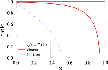
Figure 7: (Color online) Influence of the phase space limitation for $\sqrt{s}=$7 GeV and $\ell_{t}=$ .3 GeV. We display the ratio $\int P_{g}\Theta(k_{\mathrm{max}}-k_{t})d^{2}\vec{k}_{t}/\int P_{g}d^{2}\vec{k}_{t}$ , the right hand side of eq. IV.1 divided by the right hand side of eq. 28, for charm and bottom quarks.

The integrated gluon distribution, eq. 28, depends on $\vec{\ell}_{t}^{2}$ and $x^{2}M^{2}$ through the ratio $\vec{\ell}_{t}^{2}/(x^{2}M^{2})$ only. For hard scattering, when this ratio is large, the limiting form of eq. 28 is given by

$$\int P_{g}d^{2}\vec{k}_{t}\sim 2\frac{C_{A}\alpha_{s}}{\pi}\frac{1-x}{x}\log\frac{\vec{\ell}_{t}^{2}}{x^{2}M^{2}},$$ (29)

which shows the logarithmic enhancement mentioned at the beginning of section III. For soft scattering, when the ratio $\vec{\ell}_{t}^{2}/(x^{2}M^{2})$ is small, the limiting form is

$$\int P_{g}d^{2}\vec{k}_{t}\sim\frac{C_{A}\alpha_{s}}{\pi}\frac{1-x}{x}\frac{2\,\vec{\ell}_{t}^{2}}{3\,x^{2}M^{2}}.$$ (30)

The proportionality of the result to $\vec{\ell}_{t}^{2}/(x^{2}M^{2})$ is evident from the approximate constancy of $\mathcal{I}$ in this regime, eq. 24, up to $\vec{k}_{t}^{2}\sim x^{2}M^{2}$. The hard scattering approximation of the spectrum, eq. 19, supplemented with a cut-off $\vec{k}_{t}^{2}<\vec{\ell}_{t}^{2}$, is completely off as it would result in a proportionality of the result to $(\vec{\ell}_{t}^{2}/(x^{2}M^{2}))^{2}$. This sheds a complementary light to the discussion carried out in section III.2 on the dead cone effect. In eq. 30 the radiation is in proportion to the square of the transverse momentum transfer, as expected. It is comparatively weak as compared to the hard scattering regime as a consequence of a strong destructive interference in the soft regime. A simple interpolation between these two limiting forms has been advanced in Peigne:2008wu

$$\int P_{g}d^{2}\vec{k}_{t}\approx 2\frac{C_{A}\alpha_{s}}{\pi}\frac{1-x}{x}\log\left(1+\frac{\vec{\ell}_{t}^{2}}{3\,x^{2}M^{2}}\right).$$ (31)

This expression approximates the full result, eq. 28, with a deviation smaller than 3% over the full range of $\vec{\ell}_{t}^{2}/(x^{2}M^{2})$. This is the approximation we will consider in all subsequent comparisons.

IV.2 Power spectrum

In order to calculate the power spectrum we come back to the radiation cross section eq. 8. We have to integrate it first over $\vec{k}_{t}$ as detailed above for the gluon distribution $P_{g}$ and next over the momentum transfer $\vec{\ell}_{t}$. Thus, from

$$\frac{d\sigma}{dx}=\int\frac{d\sigma^{Qq\to Qgq}}{dxd^{2}k_{t}d^{2}\ell_{t}}d^{2}\vec{k}_{t}d^{2}\vec{\ell}_{t},$$ (32)

we obtain the fractional momentum loss spectrum $x\,d\sigma/dx$. At high-energy, in the frame of the heat bath where non zero components of the target parton momentum $q$ are of order $T$, we have

$$P^{0}\approx p^{0}\quad\mathrm{and}\quad k^{0}\approx x\,p^{0},$$ (33)

(even at small $x\sim k_{q}\equiv\vec{k}_{t}^{2}/(2xp\cdot q)$, we benefit from the strong hierarchy $p^{0}\gg q^{0}$ in this frame) thus

$$x\frac{d\sigma}{dx}\approx\left(\frac{k^{0}}{P^{0}}\right)_{\mathrm{HB}}\frac{d\sigma}{dx},$$ (34)

justifying the identification of $x\,d\sigma/dx$ as a (fractional) energy loss spectrum. For $k_{\mathrm{max}}\to\infty$ we obtain a simple formula for the fractional energy loss spectrum

$$x\frac{d\sigma}{dx}=\frac{4C_{A}C_{F}}{N_{c}}\alpha_{s}^{3}(1-x)\frac{\log(\frac{3x^{2}M^{2}}{\mu^{2}})}{3x^{2}M^{2}-\mu^{2}}=\sigma_{\rm el}\,\frac{dI}{dx}\,,$$ (35)

where

$$\sigma_{\rm el}=\frac{C_{F}}{2N_{c}}\int\frac{4\alpha_{s}^{2}}{(\vec{\ell}_{t}^{2}+\mu^{2})^{2}}\;d^{2}\vec{\ell}_{t}=\frac{4\pi C_{F}\alpha_{s}^{2}}{2N_{c}\mu^{2}}$$ (36)

is the elastic $Qq\to Qq$ cross section and where

$$\frac{dI}{dx}=\frac{2C_{A}}{\pi}\alpha_{s}(1-x)\frac{\log(\frac{3x^{2}M^{2}}{\mu^{2}})}{\frac{3x^{2}M^{2}}{\mu^{2}}-1}$$ (37)

is the differential fractional energy loss spectrum per elastic collision. At small $x$ the hard scattering regime may be recognized with a behavior that can be traced back to that of the integrated gluon distribution, see eq. (29). At larger $x$ the soft scattering regime takes over with a power-law suppression $\sim 1/x^{2}$, while the factor $1-x$ comes as an additional suppression factor. The transition between the two regimes is at $x_{M}=\frac{1}{\sqrt{3}}\mu/M$.

The cross section then allows for calculating an approximate value of the energy loss per unit length due to radiation, assuming all partons of the medium to be quasi static (and neglecting coherence effects of the LPM type):

$$\frac{dE_{\rm rad}}{dz}\approx\rho\int\omega\frac{d\sigma}{d\omega}d\omega\approx\rho E_{\rm beam}\int x\frac{d\sigma}{dx}dx.$$ (38)

The integral $\int x\frac{d\sigma}{dx}dx$ has no simple form but behaves as $\sim(\mu/M)\times 1/\mu^{2}$. This scaling law can be worked out by breaking the integral of $\frac{dI}{dx}$ into two pieces, the first encompassing the hard regime and the second for the soft one. Making the appropriate approximations in both regimes, it is found that both parts contribute equally when $\mu\ll M$, leading quantitatively to $\int\frac{dI}{dx}dx\approx 4\,x_{M}\,(2C_{A}\alpha_{s}/\pi)$ up to a factor increasing from 0.5 when $M=\mu$ to 1.2 when $M\to\infty$. For a small quark mass $M<\mu$, i.e. for larger values of $x_{M}$, the dependence becomes logarithmic. From this discussion it is clear that the radiation depends strongly on the infrared cut-off $\mu$ introduced in the matrix element for the elastic collisions.

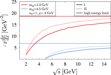
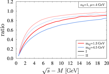
Figure 8: (Color online) Left: Integrated fractional energy loss $\int x\frac{d\sigma}{dx}\,dx$ as a function of $\sqrt{s}$ for models I and II as well as for the high energy limit eq. 35. Right: The same divided by the high-energy limit as a function of $\sqrt{s}-M$.

In fig. 8 left, the integrated fractional energy loss $\int(xd\sigma/dx)\,dx$, corresponding to the energy loss per unit length normalized to $\rho E_{\rm beam}$, is shown as a function of $\sqrt{s}$. Model I and model II take finite $s$ corrections into account (see Sect. II.2) and are compared to the $s$-independent integral of the high-energy approximation eq. (35). For the charm quark the full calculation, model I, reaches 50% of the high-energy limit at $\sqrt{s}=4.5$ GeV and 75% at $\sqrt{s}=10$ GeV. It is also seen that model II sits halfway between model I and the asymptotic result. In the right panel, the same quantity normalized to the high-energy limit is displayed as a function of $\sqrt{s}-M$ in order to better judge the influence of the heavy quark mass. As it turns out, the phase space limitation explains roughly half of the difference between model I and the high-energy limit and has the advantage to allow for an easy implementation.

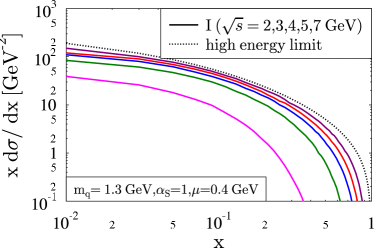
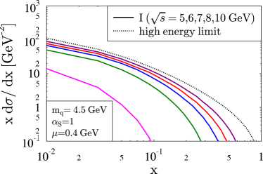
Figure 9: (Color online) The gluon emission cross section, $x\frac{d\sigma}{dx}$, for a charm quark (left) and a bottom quark (right) for several values of $\sqrt{s}$. We display the results of model I and of the high-energy formula eq. 35.

Fig. 9 shows the $x$-weighted differential energy loss cross section $xd\sigma/dx$ calculated with the full SQCD matrix element squared as compared to the approximation eq. 35. The calculation is performed for several values of $\sqrt{s}$. We observe that the approximate spectrum, eq. 35, describes the trend, shown by the SQCD calculation, quite well at low $x$ values, $0.01\leq x\leq 0.2$, where the deviation is roughly constant and less than 50% for $\sqrt{s}$ above 4.5 GeV. This explains the result seen in fig. 8, remembering that the median of $xd\sigma/dx$ is roughly given by $x_{M}$ (about $0.2$ for charm and $0.05$ for bottom). The phase space suppression at large $x$ plays an even larger role and makes the emission of an energetic gluon an even rarer process for the complete spectrum than it is when finite-$s$ corrections are ignored.

The semi-quantitative description of the full result by the high-energy approximation is welcomed for the phenomenology of quenching which is dominated by the emission of low energy gluons Baier:2001yt . Fig. 10 shows the ratio model II over model I, for the quantity $x\frac{d\sigma}{dx}$, as a function of $x$ and for several center of mass energies. We observe that model II (in which only the boundaries of the $(x,\vec{k}_{t},\vec{\ell}_{t})$ space are $s$-dependent) provides a reasonable approximation of the full result, model I, in a large interval of $x$, except at large $x$ or at rather small energies.

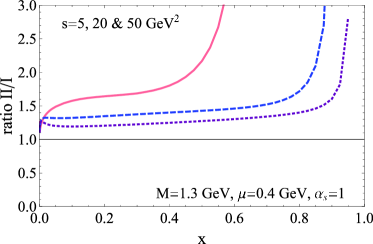
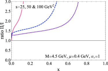
Figure 10: (Color online) Ratio of the result of model II to the result of model I for the quantity $x\frac{d\sigma}{dx}$ for charm (left) and bottom (right), plain and short-dashed lines correspond to the smallest and the largest values of $s$ in the set, respectively.

V Finite gluon mass

In the plasma the gluon is not a free particle since it is in interaction with the plasma environment. Lacking a tractable theory of how this modifies the rules used to compute the collisional and the radiative cross sections we are bound to speculate on the main phenomenological effects that could modify our results so far. In Ref. Gossiaux:2008jv , for the study of collisional losses within an approach inspired by that of Braaten and Thoma Braaten:1991jj , the effect of Debye screening was found to have a large impact on the values obtained for the energy loss. In the above results, the regularization of the elastic amplitude with the introduction of a mass parameter $\mu$ mimicked in a certain way the screening phenomenon due to a gluon thermal mass. Of course, the consequences of the occurrence of a thermal mass is not limited to the addition of a regulator in some of the propagators. With the aim of making a comparison between collisional and radiative energy losses where thermal mass effects are treated on a similar footing we want to explore the possible importance of a gluon mass on radiation.

To do so we employ a simple approach. We start out from the SQCD matrix elements and retain only the dominant terms of the series expansion in $\sqrt{s}$. Then we assume that the gluons have a finite mass $k_{\mu}k^{\mu}=m_{g}^{2}$. Going through this calculation we find that a finite gluon mass modifies only the denominator of the SQCD matrix elements and we have to replace in eqs. 14 and 18

$$x^{2}M^{2}\to x^{2}M^{2}+(1-x)m_{g}^{2}.$$ (39)

The modification of the phase space can by found in Appendix B. These modifications provide an extension of model II for finite $m_{g}$. Starting out from the hard thermal loop propagators Djordjevic et al. Djordjevic:2007at arrived recently at a similar conclusion.

Using a finite gluon mass the matrix element for gluon emission, eq. 14, does not diverge for $k_{t}\to 0$ or $k_{t}\to\ell_{t}$, even for the massless case $M=0$. Moreover, the energy loss at small $x\lesssim m_{g}/M$ – that is to say in the region of hard scattering and dead cone effect – is strongly reduced. In addition, finite gluon masses reduce the phase space and very small values of $x$ are kinematically not allowed anymore. This is seen in fig. 11 which shows for a gluon mass of $m_{g}=0,0.4$ and $0.8$ GeV the $x$-weighted differential gluon cross section $x\frac{d\sigma}{dx}$. The left panel shows the cross section for charm quarks at $\sqrt{s}=5$ GeV, the right panel that for bottom quarks at $\sqrt{s}=8$ GeV. One can extend the approximative formula, eq. 35, also toward finite gluon masses

$$x\frac{d\sigma}{dx}=4C_{F}\alpha_{s}^{3}(1-x)\frac{\log(\frac{3(m_{g}^{2}+x^{2}M^{2})}{\mu^{2}})}{3(m_{g}^{2}+x^{2}M^{2})-\mu^{2}}.$$ (40)

This formula is compared in fig. 11 with the SQCD calculation in the high energy limit. Good agreement is found for a small gluon mass only. The phase space limitations at small $x$, caused by a finite gluon mass, are indeed not contained in eq. 40.

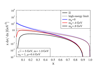
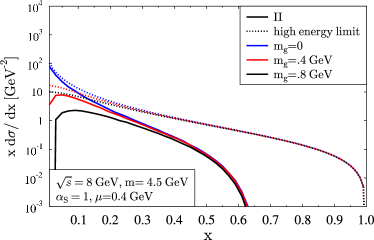
Figure 11: (Color online) Comparison of the approximate formula (eq. 40) as compared to the SQCD solution for high energies and for different gluon masses $m_{g}$. Left: $xd\sigma/dx$ of charm quarks at $\sqrt{s}=5$ GeV, right: $xd\sigma/dx$ of bottom quarks at $\sqrt{s}=8$ GeV.

The effect of a finite $m_{g}$ on the integrated fractional energy loss $\int(xd\sigma/dx)\,dx$ is shown in fig. 12. Although the gluon mass has a large effect on the absolute values, it affects only mildly the normalized quantities obtained by dividing by the high-energy limit.

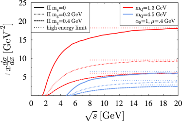
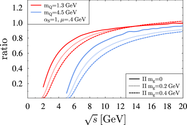
Figure 12: (Color online) Left: integrated fractional energy loss $\int xd\sigma/dx\,dx$ as a function of $\sqrt{s}$ for model II with $m_{g}=0,0.2,0.4$ GeV and $M=1.3,4.5$ GeV. Right: model II divided by the high-energy limit as a function of $\sqrt{s}$.

VI Energy loss

To close this investigation we compare the radiative and collisional energy loss of heavy quarks induced by scattering on light ones. To evaluate those, we start from the covariant expression for the infinitesimal evolution of the average 4-momentum:

$$\langle\frac{-dP^{\mu}}{d\tau}\rangle=\frac{1}{M}\int\frac{d^{3}q}{q^{0}}P\cdot qf(q)\int\frac{d\sigma}{dQ}(P-P^{\prime})^{\mu}dQ,$$ (41)

where $\tau$ is the heavy quark proper time, $dQ$ is the invariant phase space corresponding to the exit channel and $f$ is the invariant Fermi-Dirac distribution of light quarks

$$f(q)=\frac{g_{q}}{e^{(q\cdot u_{\rm HB}-\mu_{q})/T}+1},$$ (42)

with $g_{q}$ the degeneracy factor and $u_{\rm HB}$ the heat bath 4-velocity. To evaluate the average energy loss in the heat bath frame, we project eq. 41 on $u_{{\rm HB},\mu}$ and then proceed to the calculation of the integrals in the rest frame (r.f.) of the heavy quark. Concentrating on the energy lost through gluon radiation, eq. 41 simplifies to

$$\langle-\frac{dE_{\rm rad}}{d\tau}\rangle=\frac{M}{2}\int d^{3}qf_{\rm r.f.}(\vec{q})\int\frac{d\sigma}{dQ}\left[(u^{0}_{\rm HB}+|\vec{u}_{\rm HB}|\cos\theta{(\vec{u}_{\rm HB},\vec{q})})x+(u^{0}_{\rm HB}-|\vec{u}_{\rm HB}|\cos\theta{(\vec{u}_{\rm HB},\vec{q})})\frac{\vec{k}_{t}^{2}}{xM^{2}}\right]dQ\,,$$ (43)

where $u_{\rm HB}$ is here the heat bath velocity measured in the HQ rest frame, $u_{\rm HB}=(P^{0},-\vec{P})/M$. As $f_{\rm r.f.}(\vec{q})$ is centered around $\vec{q}$ such that $(u^{0}_{\rm HB}-|\vec{u}_{\rm HB}|\cos\theta{(\vec{u}_{\rm HB},\vec{q})})=0$, while $\int\frac{\vec{k}_{t}^{2}}{xM^{2}}\frac{d\sigma}{dQ}dQ$ is generically smaller than $\int x\frac{d\sigma}{dQ}dQ$ for $x\in[\mu/M,1]$ which represents the largest fraction of the integration domain, we neglect the second term in the bracket of eq. 43. Using $d\tau=\frac{M}{P^{0}}dt$, we then arrive at

$$\langle-\frac{dE_{\rm rad}}{dt}\rangle\approx\frac{M}{2}\int d^{3}qf_{\rm r.f.}(\vec{q})\left(1+\frac{|\vec{P}|}{P^{0}}\cos\theta{(\vec{u}_{\rm HB},\vec{q})}\right)\int x\frac{d\sigma}{dx}dx\,,$$ (44)

where the last factor has been discussed in the previous sections. It is then trivial to perform the angular integration on $\cos\theta{(\vec{u}_{\rm HB},\vec{q})}$ and to express the energy loss as a simple convolution on the $s$ variable. We proceed similarly for the collisional energy loss, using the SQCD expression for $\frac{d\sigma_{\rm el}}{dQ}$.

In fig. 13, we illustrate $dE/dt$ per flavour degree of freedom normalized to the heavy quark energy. A Fermi-Dirac distribution has been used, with a temperature $T=0.4~{}{\rm GeV}$ and 0 quark chemical potential $\mu_{q}$, while the screening mass $\mu$ was taken as $\sqrt{0.15}\,m_{D}\approx 0.4~{}{\rm GeV}$, in agreement with the model C of Gossiaux:2008jv . The plain and dashed lines show $m_{g}=0$ results with either model I or II for both charm and bottom quarks. Model II with $m_{g}=m_{D}/\sqrt{2}\approx 2T=0.8$ GeV is displayed as dot-dashed line. The energy loss strongly depends on the values of $\mu$ and $m_{g}$ and hence on the plasma environment in which the heavy quark moves. For our choice $\mu^{2}=0.3m_{g}^{2}$, the radiative energy loss for heavy quarks is even dominated by the collisional energy loss (short-dashed lines) for $|\vec{P}|$ up to several times the heavy quark mass.

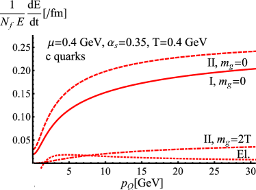
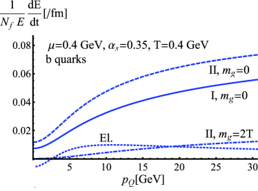
Figure 13: (Color online) Comparison between radiative and collisional energy loss of charm quarks (left) and of bottom quarks (right). Only the contribution from collisions with the light quarks of the heat bath is shown.

The radiative energy loss is calculated for the interaction of the heavy quark with the light quarks of the plasma. If one wants to add the radiation due to the interaction af a heavy quark with gluons one has to add the gluon density to the quark density in eq. 38. At high energy, this corresponds to a multiplication of the quark density by $(1+\frac{N_{f}}{6})/\frac{N_{f}}{6}$ which stems from the color factor and the flavor degrees of freedom (including quantum statistics) of $t$-channel elastic scattering of $Q-q$ and $Q-g$ Peigne:2008nd .

VII Conclusion

We present in this paper an approach to describe gluon emission from a heavy quark in collision with a light quark at mid and forward rapidity, i.e. for $x\gg k_{t}^{2}/s$. Because this radiation is centered at $x\sim k_{t}/\sqrt{s}$ and the correction are of ${\cal O}(x^{2})$ we use for this approach the scalar QCD formalism which allows identifying the physical processes much easier. We separate the matrix elements into three gauge invariant subgroups where two of them are identical with the bremsstrahlung diagrams already observed in QED. In the paper we concentrate on the third group which is genuine to QCD and dominates the radiation in the central rapidity region.

We compare the full result with a high energy approximation which can be analytically calculated and find fair agreement already for moderate $\sqrt{s}$ values ($\sqrt{s}-M\gtrsim 7\ {\rm GeV}$). In ultrarelativistic heavy ion collisions at RHIC and LHC the typical $\sqrt{s}$ value of collisions of heavy quarks with heat bath particles is lower and therefore the approximate formulas are not directly applicable. We show that the phase boundaries are responsible for a substantial part of the corrections at intermediate energies, so that a model based on asymptotic transition elements and exact phase space boundaries can be used for semi-quantitative purposes.

We find that the mass of the heavy quark suppresses the emission of gluons at low transverse momentum (dead cone effect) but this suppression is less important and less universal than originally advocated. We study the influence of a finite gluon mass on the energy loss of heavy quarks in radiative collisions and find a quite strong dependence. For massless gluons, the energy loss of heavy quarks due to radiative collisions exceeds that due to elastic collisions for all heavy quark momenta, while for massive gluons the crossing happens at moderate but finite momenta. In all cases, we conclude that radiative collisions have to be included for a quantitative description of the energy loss of heavy quarks in a quark gluon plasma. We have carried out this study assuming a constant infrared regularization scale $\mu$ for the elastic cross section and leave calculation with hard thermal loop propagators for future studies.

Appendix A Spinor QCD matrix element

For completeness we give the matrix elements for spin-$\frac{1}{2}$ quarks, $\mathcal{M}_{1}$, $\mathcal{M}_{2}$ and $\mathcal{M}_{3}$,

$$\mathcal{M}_{1} = g^{3}C_{1}\ \frac{\bar{u}(q^{\prime})\gamma^{\mu}u(q)}{(q^{\prime}-q)^{2}}D_{\mu\nu}[q^{\prime}-q]\bar{u}(P^{\prime})\frac{\gamma^{\nu}({P}\!\!\!{/}-{k}\!\!\!{/}+M){\epsilon}\!\!\!{/}}{(P-k)^{2}-M^{2}}u(P)$$

$$\mathcal{M}_{2} = g^{3}C_{2}\ \frac{\bar{u}(q^{\prime})\gamma^{\mu}u(q)}{(q^{\prime}-q)^{2}}D_{\mu\nu}[q^{\prime}-q]\bar{u}(P^{\prime})\frac{{\epsilon}\!\!\!{/}({P}\!\!\!{/}^{\prime}+{k}\!\!\!{/}+M)\gamma^{\nu}}{(P^{\prime}+k)^{2}-M^{2}}u(P)$$

$$\mathcal{M}_{3} = g^{3}C_{3}D^{\mu\mu^{\prime}}[q^{\prime}-q]D^{\nu\nu^{\prime}}[P^{\prime}-P]\Big{[}g_{\mu^{\prime}\nu^{\prime}}(P-P^{\prime}+q^{\prime}-q)_{\sigma}+g_{\nu^{\prime}\sigma}(P^{\prime}-P-k)_{\mu^{\prime}}+g_{\sigma\mu^{\prime}}(q-q^{\prime}+k)_{\nu^{\prime}}\Big{]}\epsilon^{\sigma}$$ (45)

$$\times \frac{\bar{u}(q^{\prime})\gamma^{\mu}u(q)\bar{u}(P^{\prime})\gamma^{\nu}u(P)}{(q^{\prime}-q)^{2}(P^{\prime}-P)^{2}}.$$

Appendix B Phase space

Here we calculate the three body phase space in the Sudakov variables of Sect II.2. We introduce here in addition a finite gluon mass $m_{g}$. We assume that the light quark is massless. Using $p$ and $q$ as defined in Sect II.2 and writing $k=x\,p+k_{q}\,q+k_{t}$, we note first that

$$\int d^{3}k/(2E_{k}) = \int d^{4}k\,\Theta(k^{0})\,\delta(k^{2}-m_{g}^{2})$$ (46)

$$= \int(p\cdot q)\,dx\,dk_{q}\,d^{2}k_{t}\,\Theta(x)\,\delta(2(p\cdot q)\,x\,k_{q}-\vec{k}_{t}^{2}-m_{g}^{2})$$

$$= \int dxd^{2}k_{t}\,\Theta(x)/(2x).$$

Introducing $q^{\prime}=x^{\prime}\,p+q^{\prime}_{q}\,q+q^{\prime}_{t}$ and taking into account $\ell_{t}=-q^{\prime}_{t}$, the 3-body phase space reads

$$L_{3} = \frac{1}{(2\pi)^{5}}\int d^{4}P^{\prime}\,d^{4}k\,d^{4}q^{\prime}\Theta(P^{\prime 0})\,\delta(P^{\prime 2}-M^{2})\Theta(k^{0})\,\delta(k^{2}-m_{g}^{2})\Theta(q^{\prime 0})\,\delta(q^{\prime 2})\delta(P+q-P^{\prime}-k-q^{\prime})$$ (47)

$$= \frac{1}{4\,(2\pi)^{5}}\int\frac{dx}{x}\Theta(x)d^{2}k_{t}\frac{dx^{\prime}}{x^{\prime}}\Theta(x^{\prime})d^{2}\ell_{t}\,\Theta(1-x-x^{\prime})\delta((P+q-k-q^{\prime})^{2}-M^{2}).$$

The integration over $x^{\prime}$ can be performed after writing

$$\frac{1}{xx^{\prime}}\delta\bigl{(}(P+q-k-q^{\prime})^{2}-M^{2}\bigr{)} = \delta\bigl{(}x^{\prime 2}(x\,s-\vec{k}_{t}^{2}-m_{g}^{2})-x^{\prime}(x(1-x)\,s-x\,M^{2}-\vec{k}_{t}^{2}-m_{g}^{2}+2x\,\vec{k}_{t}\cdot\vec{\ell}_{t})+x(1-x)\vec{\ell}_{t}^{2}\bigr{)}$$ (48)

$$= \frac{\Theta(\Delta)}{\sqrt{\Delta}}\bigl{\{}\delta(x^{\prime}-x^{\prime}_{1})+\delta(x^{\prime}-x^{\prime}_{2})\bigr{\}},$$

with

$$\Delta=\bigl{(}x(1-x)\,s-x\,M^{2}-\vec{k}_{t}^{2}-m_{g}^{2}+2x\,\vec{k}_{t}\cdot\vec{\ell}_{t}\bigr{)}^{2}-4x(1-x)\,\vec{\ell}_{t}^{2}\,(x\,s-\vec{k}_{t}^{2}-m_{g}^{2}).$$ (49)

Among the two roots, $x^{\prime}_{1}$ and $x^{\prime}_{2}$, one is of order 1 and the other is of order $\vec{\ell}_{t}^{2}/s$. Only the latter is relevant at high-energy, because of the suppression by the elastic matrix element at large $|t|$ and since $t=\ell^{2}=(q-q^{\prime})^{2}=-x^{\prime}\,(2p\cdot q)$. For completeness we also give the boundaries in explicit forms:

$$0\leq x \leq 1-M^{2}/s,$$

$$\vec{k}_{t}^{2} \leq x(1-x)\,s-x\,M^{2}-m_{g}^{2},$$

$$|\vec{\ell}_{t}| \leq \frac{x(1-x)\,s-x\,M^{2}-\vec{k}_{t}^{2}-m_{g}^{2}}{2\left(\sqrt{x(1-x)(x\,s-\vec{k}_{t}^{2}-m_{g}^{2})}-x\,|\vec{k}_{t}|\cos\phi\right)}.$$ (50)

Appendix C Comparison between the QCD and the QED-like gluon distributions

Here we want to further investigate the comparison between the gluon distribution eq. 15 as deduced from eq. 14 and the QED-like one that could be deduced from eq. 18. Our aim is to extract the gross features in limiting regimes in order to prove that the QED-like terms contribute only little to radiation. The discussion thus follows from the one given when commenting Fig. 2.

Again the discussion is carried out for $\mathcal{I}$, the $\phi_{k_{t}}$-integrated gluon distribution, which is made explicit in eq. 21 and will be referred to as the QCD distribution. The QED-like distribution is deduced from eq. 21 by changing $\vec{\ell}_{t}\to x\,\vec{\ell}_{t}$ and $C_{A}\to C_{F}$. For simplicity the distributions will be shown omitting their color factors and the common prefactor $\frac{2\alpha_{s}}{\pi}\frac{1-x}{x}$. Since we are mostly interested in the comparison between the QCD and the QED-like distributions the common prefactor is inessential.

The parameter space $(\ell_{t},M)$ can be split into two parts. When $M<\ell_{t}$ the regime is hard for every $x$ for the QCD distribution (since $M<\ell_{t}\Rightarrow x\,M<\ell_{t}$). We recall that in such regime we have (assuming a strong hierarchy of scales)

• $\mathcal{I}\propto 1/\vec{\ell}_{t}^{2}$ (here and in the following the constant of proportionality is the color factor times the common prefactor which we decided to skip) at small $k_{t}$, $k_{t}\ll(xM)^{2}/\ell_{t}$;

• $\mathcal{I}\propto\vec{k}_{t}^{2}/(xM)^{4}$ in the dead-cone region $(xM)^{2}/\ell_{t}\ll k_{t}\ll xM$;

• $\mathcal{I}\propto 1/\vec{k}_{t}^{2}$ in the log-enhanced region $xM\ll k_{t}\ll\ell_{t}$;

• $\mathcal{I}\propto\vec{\ell}_{t}^{2}/(\vec{k}_{t}^{2})^{2}$ at large $k_{t}$, $k_{t}\gg\ell_{t}$.

Figure 14: (Color online) $k_{t}$ distribution of gluons $\mathcal{I}(x,|\vec{k}_{t}|,t;M)$ for the QCD (thick lines) and the QED-like cases. Left (hard scattering only): $|\vec{\ell}_{t}|=1$, $M=0.1$ and $x=0.3$. Right : $|\vec{\ell}_{t}|=1$, $M=3.$; $x_{1}=0.5$ (dashed lines; soft scattering) and $x_{1}=0.01$ (solid lines).

This trend is visible in Fig. 14 (left) which shows the QCD distribution (thick line). The QED-like distribution is also shown for comparison (thin line). For $M<\ell_{t}$ the regime is also hard for the latter, since $x\,M<x\,\ell_{t}$. Therefore the same sequence of behavior is obtained but the change of $\ell_{t}$ by $x\,\ell_{t}$ squeezes the intermediate range. Both curves are on top of each other in both, the dead-cone and the log-enhanced windows, since the function there is $\ell_{t}$-independent. With the above-mentioned squeezing the log-enhanced window is shorten in the QED-like case and therefore the QED-like distribution becomes negligible for $k_{t}>x\,\ell_{t}$. A further consequence is that the $k_{t}$-integrated distribution is $\propto\ln(\ell_{t}/M)$ for the QED-like case to be compared with $\ln(\ell_{t}/(x\,M))$ for the QCD case, hence the dominance of the QCD distribution at small $x$. At small $k_{t}$ the squeezing of the dead-cone window results in the dominance of the QED distribution which is $\propto 1/(x^{2}\vec{\ell}_{t}^{2})$. This region is irrelevant for the whole radiation as the $k_{t}$-integration demonstrates.

When $M>\ell_{t}$, the regime is soft for the QED-like distribution, as $x\,\ell_{t}<x\,M$. For the QCD distribution, as thoroughly investigated in the main part of the paper, the regime is hard at small $x$ when $x\,M<\ell_{t}$ and becomes soft for larger $x$. We recall that the soft regime for the QCD distribution is characterized by

• $\mathcal{I}\propto\vec{\ell}_{t}^{2}/(x\,M)^{4}$ at small $k_{t}$, $k_{t}\ll x\,M$;

• $\mathcal{I}\propto\vec{\ell}_{t}^{2}/(\vec{k}_{t}^{2})^{2}$ at large $k_{t}$, $k_{t}\gg x\,M$.

The various possibilities are plotted in Fig. 14 (right). The thick red dashed line is the QCD distribution for a typical large $x$ value, $x=x_{1}$ (soft regime), and the thin red dashed line is the QED-like distribution for the same $x=x_{1}$. From the above behaviors and the change $\ell_{t}\to x\,\ell_{t}$ when going from QCD to QED-like we see that the QED-like distribution is simply scaled down by a factor $x^{2}$ with respect to the QCD one (property C). This simple scaling translates to the $k_{t}$-integrated distributions, being respectively $\propto\vec{\ell}_{t}^{2}/(x\,M)^{2}$ and $\vec{\ell}_{t}^{2}/M^{2}$ for the QCD and QED-like situations. At smaller $x$, $x=x_{2}$, the trend is exemplified in Fig. 14 (right) with the thick black curve (QCD) and the thin black curve (QED-like). For $x<\vec{\ell}_{t}^{2}/M^{2}$ ($x_{2}$ was chosen in this range), the QED-like distribution overshoots the QCD one at small $k_{t}$, precisely when $k_{t}<x\,\ell_{t}$. This is the property B pointed out in Sect. III.2 – with $l_{t}$ taken as $\mu$ – when discussing the ratio ${\bar{P}}_{g}^{SQED}/{\bar{P}}_{g}^{tot}$. As already mentioned this overshooting is harmless for the overall radiation. For $\vec{\ell}_{t}^{2}/M^{2}<x<\ell_{t}/M$, the curves (not plotted) show the same trend as the solid curves in Fig. 14 (right) but the QCD distribution is always greater than the QED-like one, with however a sizable ratio $\mathcal{O}\left(\frac{l_{t}^{2}}{xM^{2}}\right)^{2}$ provided $k_{t}\lesssim\frac{(xM)^{2}}{l_{t}}$ (property A).

References

- (1) S. Borsanyi, G. Endrodi, Z. Fodor, A. Jakovac, S. D. Katz, S. Krieg, C. Ratti and K. K. Szabo, JHEP 1011, 077 (2010).
- (2) A. Andronic, P. Braun-Munzinger, K. Redlich, J. Stachel, Nucl.Phys.A 789, 334 (2007).
- (3) R. Vogt, Int. J. Mod. Phys. E 12, 211 (2003).
- (4) M. Cacciari, P. Nason, R. Vogt, Phys. Rev. Lett. 95, 122001 (2005)
- (5) M. Cacciari, S. Frixione, N. Houdeau, M. L. Mangano, P. Nason, G. Ridolfi, JHEP 10, 137 (2012).
- (6) PHENIX Collaboration (A. Adare et al.), Phys. Rev.C 84, 044905 (2011).
- (7) ALICE Collaboration (B. Abelev et al.), JHEP 09, 112 (2012).
- (8) P. B. Gossiaux, S. Vogel, H. van Hees, J. Aichelin, R. Rapp, M. He and M. Bluhm, arXiv:1102.1114 [hep-ph].
- (9) J. D. Bjorken, Fermilab preprint Pub-82/59-THY (1982).
- (10) E. Braaten and M. H. Thoma, Phys. Rev. D 44, 1298 (1991); Phys. Rev. D 44, 2625 (1991).
- (11) A. Peshier, Phys. Rev. Lett. 97, 212301 (2006).
- (12) S. Peigne and A. Peshier, Phys. Rev. D 77, 114017 (2008).
- (13) P. B. Gossiaux and J. Aichelin, Phys. Rev. C 78, 014904 (2008); J. Phys. G 36, 064028 (2009).
- (14) M. Gyulassy and X.-N. Wang, Nucl. Phys. B 420, 583 (1994).
- (15) X.-N. Wang, M. Gyulassy, and M. Plümer, Phys. Rev. D 51, 3436 (1995).
- (16) R. Baier, Y. L. Dokshitzer, S. Peigné, and D. Schiff, Phys. Lett. B 345, 277 (1995).
- (17) R. Baier, Y. L. Dokshitzer, A. H. Müller, S. Peigné, and D. Schiff, Nucl. Phys. B 478, 577 (1996); ibid. 483, 291 (1997); ibid. 484, 265 (1997).
- (18) B. G. Zakharov, JETP Lett. 63,952 (1996) ; ibid. 65, 615 (1997); ibid. 73, 49 (2001); Phys. Atom. Nucl. 61, 838 (1998) [Yad. Fiz. 61, 924 (1998)].
- (19) M. Gyulassy, P. Levai, and I. Vitev, Phys. Rev. Lett. 85, 5535 (2000); Nucl. Phys. B 571, 197 (2000); ibid. 594, 371 (2001).
- (20) Y. L. Dokshitzer and D. E. Kharzeev, Phys. Lett. B 519, 199 (2001).
- (21) P. B. Arnold, G. D. Moore, and L. G. Yaffe, JHEP 0011, 001 (2000); ibid. 0305, 051 (2003).
- (22) B. G. Zakharov, JETP Lett. 80, 617 (2004)
- (23) N. Armesto, C. A. Salgado, and U. A. Wiedemann, Phys. Rev. D 69, 114003 (2004); Phys. Rev. C 72, 064910 (2005).
- (24) B.-W. Zhang, E.Wang and X.-N.Wang, Phys. Rev. Lett. 93, 072301 (2004).
- (25) M. Djordjevic and M. Gyulassy, Nucl.Phys. A 733, 265 (2004); M. Djordjevic, M. Gyulassy and S.Wicks, Phys. Rev. Lett. 94, 112301 (2005).
- (26) S. Wicks, W. Horowitz, M. Djordjevic and M. Gyulassy, Nucl. Phys. A 783, 493 (2007)
- (27) R. Baier, D. Schiff and B. G. Zakharov, Ann. Rev. Nucl. Part. Sci. 50, 37 (2000).
- (28) R. Baier, Y. L. Dokshitzer, A. H. Mueller and D. Schiff, Phys. Rev. C 58, 1706 (1998).
- (29) B.G. Zakharov, arxiv :hep-ph/9807396v1.
- (30) P. B. Arnold, G. D. Moore and L. G. Yaffe, JHEP 0206, 030 (2002).
- (31) P. B. Gossiaux, R. Bierkandt and J. Aichelin, Phys. Rev. C 79, 044906 (2009).
- (32) P. F. Kolb and U. W. Heinz, In *Hwa, R.C. (ed.) et al.: Quark gluon plasma*, 634-714
- (33) P. B. Gossiaux, J. Aichelin, T. Gousset and V. Guiho, Phys. G 37, 094019 (2010).
- (34) J. F. Gunion and G. Bertsch, Phys. Rev. D 25, 746 (1982).
- (35) O. Fochler, J. Uphoff, Z. Xu and C. Greiner, arXiv:1302.5250.
- (36) M. Djordjevic and U. Heinz, Phys. Rev. C 77, 024905 (2008).
- (37) K. Werner, I. Karpenko, T. Pierog, M. Bleicher and K. Mikhailov, Phys. Rev. C 82, 044904 (2010).
- (38) K. Werner, I. Karpenko, M. Bleicher, T. Pierog and S. Porteboeuf-Houssais, Phys. Rev. C 85, 064907 (2012).
- (39) P. B. Gossiaux, J. Aichelin, M. Bluhm, T. Gousset, M. Nahrgang, S. Vogel and K. Werner, PoS QNP 2012, 160 (2012).
- (40) C. Itzykson and J.-B. Zuber, Quantum Field Theory, Dover Publications, Mineola, New York (2005).
- (41) E. Meggiolaro, Phys. Rev. D 53, 3835 (1996).
- (42) P. J. Silva, O. Oliveira, P. Bicudo, N. Cardoso, arXiv:1310.5629.
- (43) A. Peshier, arxiv: hep-ph/0601119.
- (44) S. Peigne and A. V. Smilga, Phys. Usp. 52, 659 (2009) [Usp. Fiz. Nauk 179, 697 (2009)].
- (45) R. Baier, Y. L. Dokshitzer, A. H. Mueller and D. Schiff, JHEP 0109, 033 (2001).