A class of exactly solvable models for the Schrödinger equation

Abstract

We present a class of confining potentials which allow one to reduce the one-dimensional Schrödinger equation to a named equation of mathematical physics, namely either Bessel’s or Whittaker’s differential equation. In all cases, we provide closed form expressions for both the symmetric and antisymmetric wavefunction solutions, each along with an associated transcendental equation for allowed eigenvalues. The class of potentials considered contains an example of both cusp-like single wells and a double-well.

I Introduction

Exact solutions of the steady-state one-dimensional Schrödinger equationSchrodinger for a particle of mass $m$, energy $E$, and with an external potential $V(x)$,

$$\frac{-\hbar^{2}}{2m}\frac{d^{2}}{dx^{2}}\psi(x)+V(x)\psi(x)=E\psi(x),$$ (1)

are not only of a purely mathematical interest or useful as a testbed of numerical, perturbative or semi-classical treatments, but are important to elucidate interesting physics at an analytic level of realistic systems.

Since the historic solutionsMorse ; Eckart ; Rosen ; Teller ; Manning found at the advent of quantum mechanics there has been much effort in the community to find further exact solutions,Scarf ; Loudon ; Whitehead ; Pertsch ; Wang ; Parfitt ; Bagrov either by use of special functions, or via the ideas of the factorization methodInfeld and supersymmetric quantum mechanics.Cooper ; Mallow Lately, finding quasi-exact solutions,Turbiner ; Ushveridze ; Bender ; DowningHeun ; Hartmann where only some of the eigenfunctions and eigenvalues are found explicitly, has also become a popular pursuit.

Here we investigate the following class of attractive confining potential

$$V(x)=-\frac{\hbar^{2}}{2m}U_{0}\frac{(|x|/d)^{p}}{(1+|x|/d)^{2}},\qquad p=0,1,2$$ (2)

with the parameters $U_{0}>0$ and $d>0$ describing the well depth and width respectively, and the class parameter $p$ defining either: a steep well falling as $1/|x|^{2}$ $(p=0)$; a double-well $(p=1)$; or a shallow well dropping as $1/|x|$ $(p=2)$, as we plot in Fig. 1.

We have also investigated the cases $p=-1,-2$ and found, whilst a similar change of variable to what is used here leads to a confluent Heun differential equation,Heun attempts at finding closed form solutions are frustrated by the stringent conditions required for confluent Heun polynomials.Ronveaux

Whilst the importance of single wells in physics and chemistry is well known, the double-well problem is equally interesting, with applications in areas including double-well tunneling,Gillan semiconductor heterostructures,Alferov atom transfer in a scanning tunneling microscope,Budau Bose-Einstein condensationSpekkens and instantons.Coleman

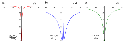
Figure 1: The class of potentials considered, Eq. (2), with (a) $p=0$, (b) $p=1$ and (c) $p=2$. Please note in (c) we have shifted the energy reference level and redefined constants, as in Eq. (18).

The rest of this work details our search for bound state $(E<0)$ solutions of Eq. (1) with the family of potentials Eq. (2), namely we solve

$$\psi^{\prime\prime}(x)+\left(U_{0}\frac{(|x|/d)^{p}}{(1+|x|/d)^{2}}-\kappa^{2}\right)\psi(x)=0,$$ (3)

where ^′ denotes taking a derivative with respect to $x$ and $\kappa^{2}=-2mE/\hbar^{2}$, for the class parameter $p=0,1,2$ in Sec. II, Sec. III and Sec. IV respectively. We draw some conclusions in Sec. V.

II Steep single well: p=0

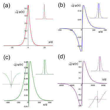
Figure 2: The four lowest eigenstates of the $p=0$ potential, with $U_{0}d^{2}=1$ and (a) $\kappa d=0.477$, (b) $\kappa d=0.0373$, (c) $\kappa d=0.0111$, and (d) $\kappa d=0.000911$. Inset: probability density. In (c) and (d) a zoom in close to the origin shows the number of nodes more clearly.

We substitute $p=0$ into Eq. (3) and find with the change of variables $\xi=\kappa d(1\pm x/d)$, where $(+)$ and $(-)$ are taken in half-axes $x>0$ and $x<0$ respectively, the following Schrödinger equation

$$\psi^{\prime\prime}(\xi)+\left(\frac{U_{0}d^{2}}{\xi^{2}}-1\right)\psi(\xi)=0.$$ (4)

Seeking a solution in the form $\psi(\xi)=\xi^{1/2}f(\xi)$ yields the modified Bessel differential equationAbramowitz

$$\xi^{2}f^{\prime\prime}(\xi)+\xi f^{\prime}(\xi)-\left(\xi^{2}+\alpha^{2}\right)f(\xi)=0,$$ (5)

with order $\alpha=\sqrt{\frac{1}{4}-U_{0}d^{2}}$. The asymptotically decaying solution is the modified Bessel function of the second kind, defined through the modified Bessel function of the first kind $I_{\alpha}(\xi)=\sum_{m=0}^{\infty}\frac{1}{m!}\frac{1}{\Gamma(m+\alpha+1)}\left(\frac{\xi}{2}\right)^{2m+\alpha}$ as followsAbramowitz

$$K_{\alpha}(\xi)=\frac{\pi}{2}\frac{I_{-\alpha}(\xi)-I_{\alpha}(\xi)}{\sin(\alpha\pi)},$$ (6)

which has the large $|\xi|$ asymptotic expansion

$$K_{\alpha}(\xi)\sim\sqrt{\frac{\pi}{2\xi}}e^{-\xi}.$$ (7)

The full solution should include two constants $c_{\pm}$ arising from the regions $x\geq 0$ and $x\leq 0$ respectively

$$\psi_{\pm}(\xi)=\frac{c_{\pm}}{\sqrt{d}}\xi^{1/2}K_{\alpha}(\xi),$$ (8)

and, upon matching these solutions and their first spatial derivatives across the boundary $x=0$, we find the odd solutions have eigenvalues defined by the transcendental equation

$$K_{\alpha}(\kappa d)=0,$$ (9)

along with the condition $c_{+}=-c_{-}$, whilst the even solutions have eigenvalues given by

$$\frac{K_{\alpha+1}(\kappa d)}{K_{\alpha}(\kappa d)}=\frac{\alpha+1/2}{\kappa d},$$ (10)

as well as the restriction $c_{+}=c_{-}$. The form of these conditions, Eq. (9) and Eq. (10), are familiar from the pioneering work of LoudonLoudon on the one-dimensional hydrogen atom.

We plot in Fig. 2 the four lowest eigenstates respectively, detailing the usual alternating symmetric and antisymmetric solutions. The advance of these four states with the system parameters $U_{0}$ and $d$ is shown in Fig. 3.

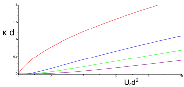
Figure 3: The progression of the four lowest eigenstates of the $p=0$ potential with system parameters $U_{0}d^{2}$, found via solutions of Eq. (9) and Eq. (10).

III Double-well: p=1

Considering a double hump potential profile, we set $p=1$ in Eq. (3). Eliminating the independent variable via the transformation $\xi=2\kappa d(1\pm x/d)$ we intermediately obtain Whittaker’s differential equationGradshteyn

$$\psi^{\prime\prime}(\xi)+\left(-\frac{1}{4}+\frac{\mu}{\xi}+\frac{\frac{1}{4}-\nu^{2}}{\xi^{2}}\right)\psi(\xi)=0.$$ (11)

where

$$\mu=\frac{U_{0}d}{2\kappa},\qquad\nu=\sqrt{\frac{1}{4}+U_{0}d^{2}}.$$ (12)

The square-integrable solution we desire is the Whittaker function of second kind, which can be constructed as followsGradshteyn

$$W_{\mu,\nu}(\xi)=\frac{\Gamma(-2\nu)}{\Gamma(\frac{1}{2}-\nu-\mu)}M_{\mu,\nu}(\xi)+\frac{\Gamma(2\nu)}{\Gamma(\frac{1}{2}+\nu-\mu)}M_{\mu,-\nu}(\xi),$$ (13)

in terms of the Whittaker function of first kind, $M_{\mu,\nu}(\xi)=\xi^{\nu+\frac{1}{2}}e^{-\frac{\xi}{2}}_{1}F_{1}\left(\frac{1}{2}+\nu-\mu;2\nu+1;\xi\right)$, where ${}_{1}F_{1}(\alpha;\beta;z)$ is a confluent hypergeometric function and $\Gamma(z)$ a gamma function. Eq. (13) decays for large $|\xi|$ as follows

$$W_{\mu,\nu}(\xi)\sim e^{-\frac{\xi}{2}}\xi^{\mu},$$ (14)

and is thus indeed a solution corresponding to a bound-state wavefunction.

Figure 4: The four lowest eigenstates of the $p=1$ potential, with $U_{0}d^{2}=1$ and (a) $\kappa d=0.408$, (b) $\kappa d=0.290$, (c) $\kappa d=0.222$, and (d) $\kappa d=0.183$. Inset: probability density.

Upon ensuring both the full solution,

$$\psi_{\pm}(x)=\frac{c_{\pm}}{\sqrt{d}}W_{\mu,\nu}(2\kappa d(1\pm x/d)),$$ (15)

and its first spatial derivative are continuous across the interface at the origin, we find the eigenvalues of antisymmetric solutions arise via

$$W_{\mu,\nu}(2\kappa d)=0,$$ (16)

which is coupled to the constraint $c_{+}=-c_{-}$. The symmetric solutions have eigenvalues governed by

$$W_{\mu,\nu}^{\prime}(\xi)\bigg{|}_{x=0}=0,$$ (17)

along with the condition $c_{+}=c_{-}$. Eqs. (16, 17) can be solved by the usual graphical or numerical methods and the remaining normalization constant $c_{+}$ is found by square-integrating over the interval $(-\infty,\infty)$.

In Fig. 4 we display in our wavefunction plots the parity interchange of successive states, from the ground to the next three highest states, as expected for an even potential. The evolution of these states with modulation of the system parameters $U_{0}$ and $d$ is shown Fig. 5.

Figure 5: The progression of the four lowest eigenstates of the $p=1$ potential with system parameters $U_{0}d^{2}$, found via solutions of Eq. (16) and Eq. (17).

IV Shallow single well: p=2

When taking the $p=2$ case, we shift where we measure the reference level and redefined constants, preferring to instead consider

$$V(x)=-\frac{\hbar^{2}}{2m}U_{0}\left(1-\frac{(|x|/d)^{2}}{(1+|x|/d)^{2}}\right).$$ (18)

As in Sec. III, working in the variable $\xi=2\kappa d(1\pm x/d)$ leads to a Whittaker differential equation, but now with a transformed $\mu$ parameter

$$\mu\to\frac{U_{0}d}{\kappa}.$$ (19)

Remarkably, the $p=1$ solution Eq. (15), along with both eigenvalue conditions Eqs. (16, 17), solve this toy model problem upon making the above transformation, Eq. (19). Fig. 6 and Fig. 7 show the behavior of example eigenstates and eigenvalues respectively.

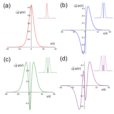
Figure 6: The four lowest eigenstates of the $p=2$ potential, with $U_{0}d^{2}=1$ and (a) $\kappa d=0.796$, (b) $\kappa d=0.532$, (c) $\kappa d=0.425$, and (d) $\kappa d=0.345$. Inset: probability density.

Differences between this shallower single well Eq. (18), compared to the steeper well of Sec. II, is most noticeable in both the inter-energy-level separation, which is smaller, and the actual values of the energy levels, which are deeper (both features are measured as a function of the ground state energy). This is simply due to the wavefunctions, in going from a steeper to a shallower well, become (relatively) extended, squeezing and lowering the energy levels of the system.

Figure 7: The progression of the four lowest eigenstates of the $p=2$ potential with system parameters $U_{0}d^{2}$.

V Discussion

The structure of the Schrödinger equation means the potential class investigated here with Eq. (2) is exactly-solvable in terms of Whittaker functions, and in fact remains so even with an additional Loudon-typeLoudon function also added

$$V(x)=-\frac{\hbar^{2}}{2m}\left(U_{0}\frac{(|x|/d)^{p}}{(1+|x|/d)^{2}}+U_{1}\frac{(|x|/d)^{q}}{(1+|x|/d)}\right),$$ (20)

$$p=0,1,2,\qquad q=0,1,$$

with the change of variable used in this work, and with only the parameters $\mu,\nu$ of the Whittaker functions being modified.

In conclusion, bound states solutions for a class of confining potential have been obtained with the one-dimensional Schrödinger equation. In constructing our solutions, we made significant use of Whittaker functionsnote to express the eigenstates, and found brief transcendental equations specify the allowed eigenvalues. Notably, the model systems include examples of both single wells and a double-well, which increases the variety of potential applications in physics and chemistry. We hope that these exact solutions will be of use in the construction of new physical models.

References

- (1) E. Schrödinger, Ann. Phys. (Leipzig) 79 361 (1926).
- (2) P. M. Morse, Phys. Rev. 34, 57 (1929).
- (3) C. Eckart, Phys. Rev. 35, 1303 (1930).
- (4) N. Rosen and P. M. Morse, Phys. Rev. 42, 210 (1932).
- (5) G. Pöschl and E. Teller, Z. Phys. 83, 143 (1933).
- (6) A list of exact solutions from the genesis of quantum mechanics is given in M. F. Manning, Phys. Rev. 48, 161 (1935).
- (7) F. Scarf, Phys. Rev. 112, 1137 (1958).
- (8) R. Loudon, Am. J. Phys. 27, 649 (1959).
- (9) R. R. Whitehead, A. Watt, G. P. Flessas and M. A. Nagarajan, J. Phys. A: Math. Gen. 15, 1217 (1982).
- (10) D. Pertsch J. Phys. A: Math. Gen. 23, 4145 (1990).
- (11) C. M. Bender and Q. Wang, J. Phys. A: Math. Gen. 34 9835 (2001).
- (12) D. G. W. Parfitt and M. E. Portnoi, J. Math. Phys. 43, 4681 (2002).
- (13) For a comprehensive list of exact solutions please see V. G. Bagrov and D. M. Gitman, Exact Solutions of Relativistic Wave Equations (Kluwer, Dordrecht, 1990).
- (14) L. Infeld and T. E. Hull, Rev. Mod. Phys. 23, 21 (1951).
- (15) F. Cooper, A. Khare, and U. P. Sukhatme, Supersymmetry in Quantum Mechanics (World Scientific, Singapore, 2001).
- (16) A. Gangopadhyaya, J. V. Mallow and C. Rasinariu, Supersymmetric Quantum Mechanics (World Scientific, Singapore, 2011), and references therein.
- (17) A. V. Turbiner, Sov. Phys. JETP 67, 230 (1988); A. Turbiner, Commun. Math. Phys. 118, 467 (1988).
- (18) A. G. Ushveridze, Quasi-exactly Solvable Models in Quantum Mechanics (Institute of Physics, Bristol, 1994).
- (19) C. M. Bender and S. Boettcher, J. Phys. A 31, L273 (1998).
- (20) C. A. Downing, J. Math. Phys. 54, 072101 (2013).
- (21) R. R. Hartmann, arXiv:1306.2836 (2013).
- (22) M. J. Gillan, J. Phys. C: Solid State Phys. 20 3621 (1987).
- (23) Z. I. Alferov, Rev. Mod. Phys. 73, 767 (2001).
- (24) P. Budau and M. Grigorescu, Phys. Rev. B 57, 6313 (1998).
- (25) R. W. Spekkens and J. E. Sipe, Phys. Rev. A 59, 3868 (1999).
- (26) S. Coleman, Aspects of Symmetry (Cambridge University Press, Cambridge, 1985).
- (27) K. Heun Math. Ann. 33, 161 (1889).
- (28) A. Ronveaux, Heun’s Differential Equations (Oxford University Press, Oxford, 1995).
- (29) M. Abramowitz and I. Stegun, Handbook of Mathematical Functions (Dover, New York, 1972).
- (30) I. S. Gradshteyn and I. M. Ryzhik, Table of Integrals, Series and Products (Academic, New York, 1980).
- (31) Markedly, the analysis in Sec. II could also be carried out with Whittaker functions, after using the identity .