An Information Theoretic Measure of
Judea Pearl’s Identifiability and Causal Influence

Abstract

In this paper, we define a new information theoretic measure that we call the “uprooted information”. We show that a necessary and sufficient condition for a probability $P(s|do(t))$ to be “identifiable” (in the sense of Pearl) in a graph $G$ is that its uprooted information be non-negative for all models of the graph $G$. In this paper, we also give a new algorithm for deciding, for a Bayesian net that is semi-Markovian, whether a probability $P(s|do(t))$ is identifiable, and, if it is identifiable, for expressing it without allusions to confounding variables. Our algorithm is closely based on a previous algorithm by Tian and Pearl, but seems to correct a small flaw in theirs. In this paper, we also find a necessary and sufficient graphical condition for a probability $P(s|do(t))$ to be identifiable when $t$ is a singleton set. So far, in the prior literature, it appears that only a sufficient graphical condition has been given for this. By “graphical” we mean that it is directly based on Judea Pearl’s 3 rules of do-calculus.

1 Introduction

For a good textbook on Bayesian networks, see, for example, the one by Koller and Friedman, Ref.[1]. We will henceforth abbreviate “Bayesian networks” by “B-nets”.

In a seminal 1995 paper (Ref.[2]), Judea Pearl defined his $do()$ operator. Then he stated and proved his 3 Rules of do-calculus. In that paper, he also defined for the first time those probabilities $P(s|do(t))$ that are identifiable (where $s$ and $t$ denote disjoint sets of visible nodes, for a given B-net whose nodes are of two kinds, either visible or unobserved.) Pearl also gave various examples of identifiable and non-identifiable probabilities $P(s|do(t))$.

Identifiable probabilities $P(s|do(t))$ can be expressed as a function of the probability distribution $P(v)$ of visible nodes. Call the act of doing this $P(v)$ expressing $P(s|do(t))$.

Later on, in Refs.[3] and [4], Tian and Pearl gave an algorithm for $P(v)$ expressing any identifiable $P(s|do(t))$, for a special type of B-net called a semi-Markovian net. They also consider B-nets that are not semi-Markovian, but that won’t concern us here as this paper will only deal with semi-Markovian nets.

Ref.[5] by Huang and Valtorta and Ref.[6] by Shpitser and Pearl have further validated the algorithm of Tian and Pearl by proving that the 3 rules of do-calculus are enough to prove the algorithm.

In this paper, we define a new, as far as we know (but read the comments about Ref.[7] below) information theoretic measure that we call the “uprooted information”. We show that a necessary and sufficient condition for a probability $P(s|do(t))$ to be identifiable in a graph $G$ is that its uprooted information be non-negative for all models of the graph $G$.

In Ref.[7], Raginsky introduced an information theoretic measure that he called “directed information” and he related it, in a loose way, to Pearl’s do-calculus. In this paper, besides the uprooted information, we also define a different quantity which we call the “information loss”. Our “information loss” is exactly equal to Raginsky’s directed-information. Thus, the uprooted information and Raginsky’s directed-information are different quantities, although they are related.

This paper connects the fields of information theory and Pearl’s identifiability in a strong way, by means of an if-and-only-if theorem, whereas Ref.[7] by Raginsky has very little to say about identifiability. Ref.[7] only mentions identifiability in its 5th and last section, and there only to connect information theory with one of the simplest possible examples of identifiability, what Pearl calls the back-door formula.

Note that Pearl’s do-calculus rules are a direct offshoot of d-separation. The Raginsky paper spends most of its time deriving some rules that are less general than Pearl’s do-calculus rules and are not stated in terms of d-separation. In fact, the Raginsky paper mentions the word “d-separation” for the first time, in italics, in the last paragraph of the paper. Contrary to the Raginsky paper, our paper will put Pearl’s do-calculus rules and d-separation front and center, ad-nauseam. In fact, this paper contains more than a dozen d-separation arguments with accompanying figures.

In this paper, we also give a new algorithm that does the same thing as the algorithm by Tian and Pearl that was mentioned above. Our algorithm is closely based on the one by Tian and Pearl, but seems to correct a small flaw in theirs. This paper includes 9 examples of B-nets to which we apply our algorithm. All examples are placed at the end of the paper, as appendices.

We also prove (in Section B.3 of this paper) that an example given in Ref.[3] by Tian and Pearl (viz., the example illustrated by Fig.9 of Ref.[3]) is actually NOT identifiable, contrary to what Ref.[3] claims! Our algorithm doesn’t get stumped by this example but the Tian and Pearl algorithm apparently does.

We also find a necessary and sufficient graphical condition for a probability $P(s|do(t))$ to be identifiable when $t$ is a singleton set. So far, in the prior literature, it appears that only a sufficient graphical condition has been given for this. By “graphical” we mean that it is directly based on Judea Pearl’s 3 rules of do-calculus.

In a future paper, we hope to generalize the measure of uprooted information to quantum mechanics by using the nowadays standard prescription of replacing probability distributions by density matrices.

2 Some Basic Notation

In this section, we will define some notation that is used throughout the paper.

Ref.[8] is a short, pedagogical introduction to Judea Pearl’s do-calculus written by Tucci, the same author as the present paper. The reader of the present paper is expected to have read Ref.[8] first, and to be thoroughly familiar with the notation of that previous paper.

As usual, ${\mathbb{Z}},{\mathbb{R}},{\mathbb{C}}$ will denote the integers, real numbers, and complex numbers, respectively. We will sometimes add superscripts to these symbols to indicate subsets of these sets. For instance, we’ll use ${\mathbb{R}}^{\geq 0}$ to denote the set of non-negative reals. For $a,b\in{\mathbb{Z}}$ such that $a\leq b$, let $Z_{a,b}=\{a,a+1,a+2,\ldots,b\}$.

Let $Bool=\{0,1\}$. Suppose $x,y\in Bool$. Let ${\overline{x}}=1-x$. Let $\wedge$ denote AND, $\vee$ denote OR, and $\oplus$ denote mod 2 addition (a.k.a. XOR). Hence

$$\begin{array}[]{c|c||c|c|c|c|}x&y&x+y&x\wedge y&x\vee y&x\oplus y\\ \hline\cr\hline\cr 0&0&0&0&0&0\\ \hline\cr 0&1&1&0&1&1\\ \hline\cr 1&0&1&0&1&1\\ \hline\cr 1&1&2&1&1&0\\ \hline\cr\end{array}\;$$ (1)

Note that one can express some of these operations in terms of others. For example, $x\wedge y=xy$, $x\vee y=x+y-xy=x\oplus y\oplus xy$, $x\oplus y=x+y-2xy$, etc.

Suppose we are given a set $(a_{j})_{\forall j\in S}$. If $T\subset S$, we will sometimes use $a_{T}$ to denote the set $(a_{j})_{\forall j\in T}$. For example, $a_{1,2,3}=(a_{1},a_{2},a_{3})$. If $a.=(a_{1},a_{2},a_{3},\ldots a_{N})$, and $j\in Z_{1,N}$, let $a_{<j}=(a_{1},a_{2},\ldots,a_{j-1})$, $a_{\leq j}=(a_{1},a_{2},\ldots,a_{j})$. $a_{>j}$ and $a_{\geq j}$ are defined in the obvious way.

Let $\delta^{x}_{y}=\delta(x,y)$ denote the Kronecker delta function: it equals 1 if $x=y$ and 0 if $x\neq y$.

In cases where $f(x)$ is a complicated expression of $x$, we will often use the abbreviation

$$\frac{f(x)}{\sum_{x}num}=\frac{f(x)}{\sum_{x}f(x)}\;.$$ (2)

Random variables will be denoted by underlined letters; e.g., ${\,\underline{a}\,}$. The (finite) set of values (a.k.a. states) that ${\,\underline{a}\,}$ can assume will be denoted by $S_{\,\underline{a}\,}$. Let $N_{\,\underline{a}\,}=|S_{\,\underline{a}\,}|$. The probability that ${\,\underline{a}\,}=a$ will be denoted by $P({\,\underline{a}\,}=a)$ or $P_{\,\underline{a}\,}(a)$, or simply by $P(a)$ if the latter will not lead to confusion in the context it is being used.

Given a known probability distribution $\{P(x)\}_{\forall x\in S_{\,\underline{x}\,}}$, we will use the following shorthand to denote the $P(x)$-weighted average of a function $f(x)$:

$$\left\langle f(x)\right\rangle_{x}=\sum_{x\in S_{\,\underline{x}\,}}P(x)f(x)\;.$$ (3)

In cases where we are dealing with several probability distributions $\{P(x)\}_{\forall x\in S_{\,\underline{x}\,}}$ and $\{Q(x)\}_{\forall x\in S_{\,\underline{x}\,}}$, and we want to make clear which one of them we are averaging over, we might replace $\left\langle f(x)\right\rangle_{x}$ by the more explicit notations $\left\langle f(x)\right\rangle_{P(x)}$ or $\left\langle f(x)\right\rangle_{P_{\,\underline{x}\,}}$.

Given two probability distributions $\{P(x)\}_{\forall x\in S_{\,\underline{x}\,}}$ and $\{Q(x)\}_{\forall x\in S_{\,\underline{x}\,}}$, the relative entropy of $P(x)$ over $Q(x)$ is defined as

$$D(P(x)//Q(x))_{\forall x\in S_{\,\underline{x}\,}}=\sum_{x\in S_{\,\underline{x}\,}}P(x)\ln\frac{P(x)}{Q(x)}\;.$$ (4)

Consider a graph $G$ with nodes ${\,\underline{x}\,}.$. Suppose ${\,\underline{b}\,}.\subset{\,\underline{B}\,}.\subset{\,\underline{c}\,}.\subset{\,\underline{x}\,}.$. Using notation which we used previously in Ref.[8], when ${\,\underline{B}\,}.$ contains ${\,\underline{b}\,}.$ and all the ancestors of ${\,\underline{b}\,}.$ in the graph $G_{{\,\underline{c}\,}.}$, we write

$${\,\underline{B}\,}.=\overline{{\,\underline{an}\,}}({\,\underline{b}\,}.,G_{{\,\underline{c}\,}.})\;.$$ (5)

In this paper, we will say that ${\,\underline{B}\,}.$ is an ancestral set in $G_{{\,\underline{c}\,}.}$ if

$${\,\underline{B}\,}.=\overline{{\,\underline{an}\,}}({\,\underline{B}\,}.,G_{{\,\underline{c}\,}.})\;.$$ (6)

Given a B-net with nodes ${\,\underline{x}\,}.=({\,\underline{x}\,}_{1},{\,\underline{x}\,}_{2},\ldots,{\,\underline{x}\,}_{N})$, suppose

$${\,\underline{x}\,}_{j(N)}\leftarrow\ldots{\,\underline{x}\,}_{j(2)}\leftarrow{\,\underline{x}\,}_{j(1)}\;$$ (7)

is a topological ordering (top-ord) of ${\,\underline{x}\,}.$. Therefore, $j(\cdot):Z_{1,N}\rightarrow Z_{1,N}$ is a permutation map. The argument of $j(\cdot)$ labels time. Hence, $j(2)$ occurs after or concurrently with $j(1)$, $j(3)$ occurs after or concurrently with $j(2)$, and so on. We will set $j(t)=\left\langle t\right\rangle$ and represent Eq.(7) by

$${\,\underline{x}\,}\left\langle N\right\rangle\leftarrow\ldots{\,\underline{x}\,}\left\langle 2\right\rangle\leftarrow{\,\underline{x}\,}\left\langle 1\right\rangle\;$$ (8)

or just by $\{{\,\underline{x}\,}{\left\langle t\right\rangle}\}_{\forall t}$. Likewise, if ${\,\underline{a}\,}.\subset{\,\underline{x}\,}.$, we will represent a top-ord of ${\,\underline{a}\,}.$ by $\{{\,\underline{a}\,}{\left\langle t\right\rangle}\}_{\forall t}$.

The Pauli matrices will be denoted by

$$\sigma_{X}=\left[\begin{array}[]{cc}0&1\\ 1&0\end{array}\right]\;\;,\;\;\sigma_{Y}=\left[\begin{array}[]{cc}0&-i\\ i&0\end{array}\right]\;\;,\;\;\sigma_{Z}=\left[\begin{array}[]{cc}1&0\\ 0&-1\end{array}\right]\;.$$ (9)

We will also have occasion to use the following 2X2 matrix, which we call the averaging matrix:

$${\cal A}=\frac{1}{2}\left[\begin{array}[]{cc}1&1\\ 1&1\end{array}\right]\;.$$ (10)

If we define $\Omega$ to be the following orthogonal matrix (real space rotation)

$$\Omega=\frac{1}{\sqrt{2}}\left[\begin{array}[]{cc}1&1\\ -1&1\end{array}\right]=e^{i\frac{\pi}{4}\sigma_{Y}}\;,$$ (11)

then ${\cal A}$ can be diagonalized as follows:

$${\cal A}=\Omega\left[\begin{array}[]{cc}0&0\\ 0&1\end{array}\right]\Omega^{T}\;.$$ (12)

More generally, if we consider the effect of $\Omega(\cdot)\Omega^{T}$ on $\left[\begin{array}[]{cc}c&f\\ g&(1+d)\end{array}\right]$ where $c,d,f,g\neq 0$, we get

$$\Omega\left[\begin{array}[]{cc}c&f\\ g&(1+d)\end{array}\right]\Omega^{T}=(1+d){\cal A}+\frac{1}{2}\left[\begin{array}[]{cc}f+g&f-g\\ g-f&-(f+g)\end{array}\right]+\frac{c}{2}\left[\begin{array}[]{cc}1&-1\\ -1&1\end{array}\right]\;.$$ (13)

${\cal A}$ is obviously real, Hermitian and a projector (${\cal A}^{2}={\cal A}$). It projects $\sigma_{X}$ to itself and the other two Pauli matrices to zero:

$${\cal A}\left\{\begin{array}[]{c}\sigma_{X}\\ \sigma_{Y}\\ \sigma_{Z}\end{array}\right\}{\cal A}=\left\{\begin{array}[]{c}\sigma_{X}\\ 0\\ 0\end{array}\right\}\;.$$ (14)

3 Visible and Unobserved Variables,
Identifiability

In this section, we will define what Judea Pearl calls “identifiability” of a quantity associated with a B-net. To define identifiability, we first have to partition the nodes of a B-net into visible and unobserved ones.

Recall our notation from Ref.[8]. A B-net with graph $G$ and nodes ${\,\underline{x}\,}.$ has a full probability distribution

$$P(x.)=\prod_{j}P(x_{j}|pa({\,\underline{x}\,}_{j}))\;.$$ (15)

Henceforth, we will refer to all B-nets with the same graph $G$ but different probability distributions $P_{{\,\underline{x}\,}.}$, as different models of $G$. Let ${\cal P}(G)$ be the set of all $P_{{\,\underline{x}\,}.}$ that can be assigned to a graph $G$. ${\cal P}(G)$ will be called the set of possible models for $G$.

Assume that ${\,\underline{x}\,}.$ equals the union of two disjoint sets ${\,\underline{u}\,}.$ and ${\,\underline{v}\,}.$. We will call the ${\,\underline{u}\,}.$ the unobserved or hidden or confounding variables. We will call the ${\,\underline{v}\,}.$ the visible or observed variables.

A function $F(x.)$ (for instance, $F(x.)=P(s.|{\stackrel{{\scriptstyle\wedge}}{{t}}}.)$) is said to be identifiable or $P_{{\,\underline{v}\,}.}$ expressible if it can be expressed as a function of $P_{{\,\underline{v}\,}.}=\{P(v.)\}_{\forall v.}$. Equivalently, $F(x.)$ is identifiable if for any two probability distributions $P^{(1)}(x.)$ and $P^{(2)}(x.)$ for the same graph $G$,

$$(\forall v.)(P^{(1)}(v.)=P^{(2)}(v.))\implies(\forall x.)(F^{(1)}(x.)=F^{(2)}(x.))\;.$$ (16)

If we define $\delta P(v.)=P^{(1)}(v.)-P^{(2)}(v.)$ and $\delta F(x.)=F^{(1)}(x.)-F^{(2)}(x.)$, then Eq.(16) can be written as

$$(\forall v.)(\delta P(v.)=0)\implies(\forall x.)(\delta F(x.)=0)\;.$$ (17)

Henceforth, if a quantity $F(x.)$ is identifiable in $G$, we will refer to the act of calculating an expression for it as a function of $P_{{\,\underline{v}\,}.}$ as $P_{{\,\underline{v}\,}.}$ expressing $F(x.)$.

Claim 1

(Lemma 13 in Ref.[3]) Suppose $G$ is a subgraph of graph $G^{+}$. Let graph $G$ (resp., $G^{+}$) have nodes ${\,\underline{x}\,}.=({\,\underline{v}\,}.,{\,\underline{u}\,}.)$ (resp., ${\,\underline{x}\,}.^{+}=({\,\underline{v}\,}.^{+},{\,\underline{u}\,}.^{+})$). Suppose ${\,\underline{s}\,}.$ and ${\,\underline{t}\,}.$ are disjoint subsets of ${\,\underline{v}\,}.$. Then

$$P(s.|{\stackrel{{\scriptstyle\wedge}}{{t}}}.)\mbox{ is identifiable in }G^{+}\implies P(s.|{\stackrel{{\scriptstyle\wedge}}{{t}}}.)\mbox{ is identifiable in }G\;$$ (18)

or, equivalently,

$$P(s.|{\stackrel{{\scriptstyle\wedge}}{{t}}}.)\mbox{ is not identifiable in }G\implies P(s.|{\stackrel{{\scriptstyle\wedge}}{{t}}}.)\mbox{ is not identifiable in }G^{+}\;.$$ (19)

In other words, the identifiability of $P(s.|{\stackrel{{\scriptstyle\wedge}}{{t}}}.)$ in a graph $G$ is inherited by the sub-graphs of $G$ (whereas un-identifiability is inherited by super-graphs).

proof:

Suppose we are given models $P^{(1)}_{G}$, $P^{(2)}_{G}$ for graph $G$ such that

$$(\forall v.)(\delta P_{G}(v.)=0)\mbox{ and }(\exists(s.,t.))(\delta P_{G}(s.|{\stackrel{{\scriptstyle\wedge}}{{t}}}.)\neq 0)\;.$$ (20)

For each $\lambda\in\{1,2\}$, define model $P^{(\lambda)}_{G^{+}}$ by setting

$$P^{(\lambda)}_{G^{+}}(x_{j}|pa({\,\underline{x}\,}_{j},G^{+}))=\left\{\begin{array}[]{l}P^{(\lambda)}_{G}(x_{j}|pa({\,\underline{x}\,}_{j},G))\mbox{ if ${\,\underline{x}\,}_{j}$ is old node; i.e., if}{\,\underline{x}\,}_{j}\in G\\ \delta_{x_{j}}^{0}\mbox{ if ${\,\underline{x}\,}_{j}$ is new node; i.e., if }{\,\underline{x}\,}_{j}\in G^{+}-G\end{array}\right.\;.$$ (21)

Since the new nodes are always constant, frozen at the same state, and there are no arrows between the new and old nodes, we can conclude from Eq.(20) that

$$(\forall v.^{+})(\delta P_{G^{+}}(v.^{+})=0)\mbox{ and }(\exists(s.,t.))(\delta P_{G^{+}}(s.|{\stackrel{{\scriptstyle\wedge}}{{t}}}.)\neq 0)\;.$$ (22)

QED

Claim 2

$P(s.|{\stackrel{{\scriptstyle\wedge}}{{t}}}.)$ is identifiable in $G_{{\,\underline{v}\,}.}$ if and only if $P(s.|{\stackrel{{\scriptstyle\wedge}}{{t}}}.)$ is identifiable in $G_{{\,\underline{v}\,}.^{-}}$ where ${\,\underline{v}\,}.^{-}=\overline{{\,\underline{an}\,}}({\,\underline{s}\,}.\cup{\,\underline{t}\,}.,G_{{\,\underline{v}\,}.})$

proof:

$$P(s.|{\stackrel{{\scriptstyle\wedge}}{{t}}}.) = \underbrace{\sum_{v.-s.}}_{\sum_{v.^{-}-s.}\sum_{v.-v.^{-}}}\left\langle\prod_{j:{\,\underline{v}\,}_{j}\in{\,\underline{v}\,}.-{\,\underline{t}\,}.}P(v_{j}|pa({\,\underline{v}\,}_{j},G_{{\,\underline{v}\,}.}),u.)\right\rangle_{u.}$$ (23a)

$$= \sum_{v.^{-}-s.}\left\langle\prod_{j:{\,\underline{v}\,}_{j}\in{\,\underline{v}\,}.^{-}-{\,\underline{t}\,}.}P(v_{j}|pa({\,\underline{v}\,}_{j},G_{{\,\underline{v}\,}.^{-}}),u.)\right\rangle_{u.}\;.$$ (23b)

Note that Eq.(23b) is identical to Eq.(23a) except that ${\,\underline{v}\,}.$ is replaced by ${\,\underline{v}\,}.^{-}$. Going from Eq.(23a) to Eq.(23b) is possible because none of the $P(v_{j}|.)$ factors make any allusion to $v.-v.^{-}$ in their “second compartment”, the one for parents.
QED

Claim 3

(Lemma 2 in Ref.[3]) When $t.=t$ is a singleton, the previous claim is true with ${\,\underline{v}\,}.^{-}$ replaced by $\overline{{\,\underline{an}\,}}({\,\underline{s}\,}.,G_{{\,\underline{v}\,}.})$.

proof:

Either ${\,\underline{t}\,}\in\overline{{\,\underline{an}\,}}({\,\underline{s}\,}.,G_{{\,\underline{v}\,}.})$, in which case $\overline{{\,\underline{an}\,}}({\,\underline{s}\,}.\cup{\,\underline{t}\,},G_{{\,\underline{v}\,}.})=\overline{{\,\underline{an}\,}}({\,\underline{s}\,}.,G_{{\,\underline{v}\,}.})$, or ${\,\underline{t}\,}\notin\overline{{\,\underline{an}\,}}({\,\underline{s}\,}.,G_{{\,\underline{v}\,}.})$, in which case $P(s.|{\stackrel{{\scriptstyle\wedge}}{{t}}})=P(s.)$ and is thus identifiable in both $G_{\overline{{\,\underline{an}\,}}({\,\underline{s}\,}.\cup{\,\underline{t}\,},G_{{\,\underline{v}\,}.})}$ and $G_{\overline{{\,\underline{an}\,}}({\,\underline{s}\,}.,G_{{\,\underline{v}\,}.})}$.
QED

Claim 4

$P(s.|{\stackrel{{\scriptstyle\wedge}}{{t}}}.)=P(s.|{\stackrel{{\scriptstyle\wedge}}{{t}}}.,(v.^{-})^{c\wedge})$ , where ${\,\underline{v}\,}.^{-}=\overline{{\,\underline{an}\,}}({\,\underline{s}\,}.\cup{\,\underline{t}\,}.,G_{{\,\underline{v}\,}.})$ and $({\,\underline{v}\,}.^{-})^{c\wedge}=({\,\underline{v}\,}.-{\,\underline{v}\,}.^{-})^{\wedge}$.

proof:

See Ref.[8] where the 3 Rules of Judea Pearl’s do-calculus are stated. Using the notation there, let ${\,\underline{b}\,}.={\,\underline{s}\,},{\,\underline{a}\,}.=({\,\underline{v}\,}.^{-})^{c},{\,\underline{h}\,}.={\,\underline{t}\,}.,{\,\underline{i}\,}.=\emptyset,{\,\underline{o}\,}.=({\,\underline{u}\,}.,{\,\underline{v}\,}.^{-}-{\,\underline{s}\,}.\cup{\,\underline{t}\,}.)$. Note that ${\,\underline{a}\,}.^{-}={\,\underline{a}\,}.-{\,\underline{an}\,}({\,\underline{i}\,}.,G_{{\stackrel{{\scriptstyle\wedge}}{{{\,\underline{h}\,}}}}.})={\,\underline{a}\,}.$ so $G_{{\stackrel{{\scriptstyle\wedge}}{{{\,\underline{h}\,}}}}.,({\,\underline{a}\,}.^{-})^{\wedge}}=G_{{\stackrel{{\scriptstyle\wedge}}{{{\,\underline{h}\,}}}}.,{\stackrel{{\scriptstyle\wedge}}{{{\,\underline{a}\,}}}}.}$. Fig.1 portrays $G_{{\stackrel{{\scriptstyle\wedge}}{{{\,\underline{h}\,}}}}.,{\stackrel{{\scriptstyle\wedge}}{{{\,\underline{a}\,}}}}.}$. Apply Rule 3 to that figure.
QED

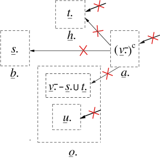
Figure 1: A portrait of $G_{{\stackrel{{\scriptstyle\wedge}}{{{\,\underline{h}\,}}}}.,{\stackrel{{\scriptstyle\wedge}}{{{\,\underline{a}\,}}}}.}$, alluded to in Claim 4

4 Uprooted Information

In this section, we will define what we call an uprooted information, and various associated quantities. In later sections, we will show that there is an intimate connection between uprooted information and identifiability.

Throughout this section, let ${\,\underline{b}\,}.,{\,\underline{a}\,}.$ and ${\,\underline{e}\,}.$ be disjoint subsets of the set ${\,\underline{x}\,}.$ of nodes of a graph $G$. We will use the following abbreviations: $I=$ information, $M=$ mutual, $C=$ conditional and $\wedge=$ uprooted. Thus, for instance, “$\wedge CMI$” will stand for “uprooted conditional mutual information”.

For all $a.,b.,e.$, we define

$$\begin{array}[]{|c|c|}\hline\cr\begin{array}[]{c}(C\mbox{ Probability })\\ P(b.|a.)\end{array}&\begin{array}[]{c}(\wedge\mbox{ Probability })\\ P(b.|{\stackrel{{\scriptstyle\wedge}}{{a}}}.)\end{array}\\ \hline\cr\begin{array}[]{c}(MI)\\ P(b.:a.)=\frac{P(b.|a.)}{P(b.)}\end{array}&\begin{array}[]{c}(\wedge MI)\\ P(b.:{\stackrel{{\scriptstyle\wedge}}{{a}}}.)=\frac{P(b.|{\stackrel{{\scriptstyle\wedge}}{{a}}}.)}{P(b.)}\end{array}\\ \hline\cr\begin{array}[]{c}(CMI)\\ P(b.:a.|e.)=\frac{P(b.|a.,e.)}{P(b.|e.)}\end{array}&\begin{array}[]{c}(\wedge CMI)\\ P(b.:{\stackrel{{\scriptstyle\wedge}}{{a}}}.|e.)=\frac{P(b.|{\stackrel{{\scriptstyle\wedge}}{{a}}}.,e.)}{P(b.|e.)}\end{array}\\ \hline\cr\end{array}\;.$$ (24)

For the case of $\wedge$ CMI, recall from Ref.[8] that $P(b.|{\stackrel{{\scriptstyle\wedge}}{{a}}}.,e.)=\frac{P(b.,e.|{\stackrel{{\scriptstyle\wedge}}{{a}}}.)}{P(e.|{\stackrel{{\scriptstyle\wedge}}{{a}}}.)}$. We also define what we call “losses” as follows:

$$\begin{array}[]{|c|}\hline\cr\begin{array}[]{c}(\wedge MI\mbox{ loss })\\ \frac{P(b.:a.)}{P(b.:{\stackrel{{\scriptstyle\wedge}}{{a}}}.)}\end{array}\\ \hline\cr\begin{array}[]{c}(\wedge CMI\mbox{ loss })\\ \frac{P(b.:a.|e.)}{P(b.:{\stackrel{{\scriptstyle\wedge}}{{a}}}.|e.)}\end{array}\\ \hline\cr\end{array}\;.$$ (25)

We will also refer by the same name to the weighted averages (over $P(x.)$) of the quantities defined in Eqs.(24) and (25), as long as it is clear from context which of the two we are referring to. So define

$$\begin{array}[]{|c|c|}\hline\cr\begin{array}[]{c}(C\mbox{ Entropy })\\ H({\,\underline{b}\,}.|{\,\underline{a}\,}.)=\left\langle 1/P(b.|a.)\right\rangle_{a.,b.}\end{array}&\begin{array}[]{c}(\wedge\mbox{ Entropy })\\ H({\,\underline{b}\,}.|{\stackrel{{\scriptstyle\wedge}}{{{\,\underline{a}\,}}}}.)=\left\langle 1/P(b.|{\stackrel{{\scriptstyle\wedge}}{{a}}}.)\right\rangle_{a.,b.}\end{array}\\ \hline\cr\begin{array}[]{c}(MI)\\ H({\,\underline{b}\,}.:{\,\underline{a}\,}.)=\left\langle P(b.:a.)\right\rangle_{a.,b.}\end{array}&\begin{array}[]{c}(\wedge MI)\\ H({\,\underline{b}\,}.:{\stackrel{{\scriptstyle\wedge}}{{{\,\underline{a}\,}}}}.)=\left\langle P(b.:{\stackrel{{\scriptstyle\wedge}}{{a}}}.)\right\rangle_{a.,b.}\end{array}\\ \hline\cr\begin{array}[]{c}(CMI)\\ H({\,\underline{b}\,}.:{\,\underline{a}\,}.|{\,\underline{e}\,}.)=\left\langle P(b.:a.|e.)\right\rangle_{a.,b.,e.}\end{array}&\begin{array}[]{c}(\wedge CMI)\\ H({\,\underline{b}\,}.:{\stackrel{{\scriptstyle\wedge}}{{{\,\underline{a}\,}}}}.|{\,\underline{e}\,}.)=\left\langle P(b.:{\stackrel{{\scriptstyle\wedge}}{{a}}}.|e.)\right\rangle_{a.,b.,e.}\end{array}\\ \hline\cr\end{array}\;,$$ (26)

and

$$\begin{array}[]{|c|}\hline\cr\begin{array}[]{c}(\wedge MI\mbox{ loss })\\ H_{loss}({\,\underline{b}\,}.:{\stackrel{{\scriptstyle\wedge}}{{{\,\underline{a}\,}}}}.)=\left\langle\frac{P(b.:a.)}{P(b.:{\stackrel{{\scriptstyle\wedge}}{{a}}}.)}\right\rangle_{a.,b.}\end{array}\\ \hline\cr\begin{array}[]{c}(\wedge CMI\mbox{ loss })\\ H_{loss}({\,\underline{b}\,}.:{\stackrel{{\scriptstyle\wedge}}{{{\,\underline{a}\,}}}}.|{\,\underline{e}\,}.)=\left\langle\frac{P(b.:a.|e.)}{P(b.:{\stackrel{{\scriptstyle\wedge}}{{a}}}.|e.)}\right\rangle_{a.,b.,e.}\end{array}\\ \hline\cr\end{array}\;.$$ (27)

As is well known, $H({\,\underline{a}\,}.:{\,\underline{b}\,}.)$ an $H({\,\underline{a}\,}.:{\,\underline{b}\,}.|{\,\underline{e}\,}.)$ must be non-negative. However, $H({\,\underline{a}\,}.:{\stackrel{{\scriptstyle\wedge}}{{{\,\underline{b}\,}.}}})$ (and thus $H({\,\underline{a}\,}.:{\stackrel{{\scriptstyle\wedge}}{{{\,\underline{b}\,}}}}.|{\,\underline{e}\,}.$ too) can be negative. For example, in Section 5, we give a graph that we call INDEF and a model for that graph such that $H({\,\underline{y}\,}:{\stackrel{{\scriptstyle\wedge}}{{{\,\underline{x}\,}}}})=-\ln(2)$. On the other hand, what we call losses are always non-negative because they can be expressed as weighted averages of relative entropies. Indeed,

$$H_{loss}({\,\underline{b}\,}.:{\stackrel{{\scriptstyle\wedge}}{{{\,\underline{a}\,}}}}.|{\,\underline{e}\,}.)=\sum_{a.,e.}P(a.,e.)D[P(b.|a.,e.)//P(b.|{\stackrel{{\scriptstyle\wedge}}{{a}}}.,e.)]_{\forall b.}\geq 0\;.$$ (28)

Note also that the $\wedge$CMI, , $\wedge$CMI loss and CMI are related by

$$H({\,\underline{b}\,}.:{\stackrel{{\scriptstyle\wedge}}{{{\,\underline{a}\,}}}}.|{\,\underline{e}\,}.)+\underbrace{H_{loss}({\,\underline{b}\,}.:{\stackrel{{\scriptstyle\wedge}}{{{\,\underline{a}\,}}}}.|{\,\underline{e}\,}.)}_{\geq 0}=\underbrace{H({\,\underline{b}\,}.:{\,\underline{a}\,}.|{\,\underline{e}\,}.)}_{\geq 0}\;.$$ (29)

Claim 5

For any graph $G$, there exists a model of $G$ such that $H({\,\underline{s}\,}.:{\stackrel{{\scriptstyle\wedge}}{{{\,\underline{t}\,}}}}.)=H({\,\underline{s}\,}.:{\,\underline{t}\,}.)=0$.

proof:

Consider any model of $G$ that satisfies: for all $j$ such that ${\,\underline{x}\,}_{j}\in{\,\underline{x}\,}.$, $P(x_{j}|pa({\,\underline{x}\,}_{j}))=P(x_{j}|pa({\,\underline{x}\,}_{j})-{\,\underline{t}\,}.)$. For such a model, all arrows exiting all nodes in node set ${\,\underline{t}\,}.$ can be erased. Hence, $H({\,\underline{s}\,}.:{\stackrel{{\scriptstyle\wedge}}{{{\,\underline{t}\,}}}}.)=H({\,\underline{s}\,}.:{\,\underline{t}\,}.)=0$.
QED

The sign of the uprooted information $H({\,\underline{s}\,}.|{\stackrel{{\scriptstyle\wedge}}{{{\,\underline{t}\,}}}}.)$ obeys the following simple inheritance property analogous to the inheritance property (Claim 1) for identifiability.

Claim 6

Suppose $G$ is a subgraph of graph $G^{+}$. Let graph $G$ (resp., $G^{+}$) have nodes ${\,\underline{x}\,}.=({\,\underline{v}\,}.,{\,\underline{u}\,}.)$ (resp., ${\,\underline{x}\,}.^{+}=({\,\underline{v}\,}.^{+},{\,\underline{u}\,}.^{+})$). Suppose ${\,\underline{s}\,}.$ and ${\,\underline{t}\,}.$ are disjoint subsets of ${\,\underline{v}\,}.$. Let $P_{G}$ (resp., $P_{G^{+}}$) denote a model for $G$ (resp., $G^{+}$). Then

$$(\forall P_{G^{+}})(H_{P_{G^{+}}}({\,\underline{s}\,}.|{\stackrel{{\scriptstyle\wedge}}{{{\,\underline{t}\,}}}}.)\geq 0)\implies(\forall P_{G})(H_{P_{G}}({\,\underline{s}\,}.|{\stackrel{{\scriptstyle\wedge}}{{{\,\underline{t}\,}}}}.)\geq 0)\;$$ (30)

or, equivalently,

$$(\exists P_{G})(H_{P_{G}}({\,\underline{s}\,}.|{\stackrel{{\scriptstyle\wedge}}{{{\,\underline{t}\,}}}}.)<0)\implies(\exists P_{G^{+}})(H_{P_{G^{+}}}({\,\underline{s}\,}.|{\stackrel{{\scriptstyle\wedge}}{{{\,\underline{t}\,}}}}.)<0)\;$$ (31)

proof:

Suppose we are given a $G$ model $P_{G}(x.)$ such that $H_{P_{G}}({\,\underline{s}\,}.|{\stackrel{{\scriptstyle\wedge}}{{{\,\underline{t}\,}}}}.)<0$. Define a $G^{+}$ model $P_{G^{+}}(x.)$ by setting

$$P_{G^{+}}(x_{j}|pa({\,\underline{x}\,}_{j},G^{+}))=\left\{\begin{array}[]{l}P_{G}(x_{j}|pa({\,\underline{x}\,}_{j},G))\mbox{ if ${\,\underline{x}\,}_{j}$ is old node; i.e., if}{\,\underline{x}\,}_{j}\in G\\ \delta_{x_{j}}^{0}\mbox{ if ${\,\underline{x}\,}_{j}$ is new node; i.e., if }{\,\underline{x}\,}_{j}\in G^{+}-G\end{array}\right.\;.$$ (32)

Since the new nodes are always frozen at the same state, and all the arrows between the old and new nodes can be erased, we can conclude that $H_{P_{G^{+}}}({\,\underline{s}\,}.|{\stackrel{{\scriptstyle\wedge}}{{{\,\underline{t}\,}}}}.)<0$.
QED

Even though $H({\,\underline{b}\,}_{2},{\,\underline{b}\,}_{1}:{\,\underline{a}\,}.)\geq H({\,\underline{b}\,}_{1}:{\,\underline{a}\,}.)$, note that

$$\mbox{ Not true: }H({\,\underline{b}\,}_{2},{\,\underline{b}\,}_{1}:{\stackrel{{\scriptstyle\wedge}}{{{\,\underline{a}\,}}}}.)\geq H({\,\underline{b}\,}_{1}:{\stackrel{{\scriptstyle\wedge}}{{{\,\underline{a}\,}}}}.)\;.$$ (33)

For example, for the graph of Fig.13, $H({\,\underline{y}\,},{\,\underline{z}\,}:{\stackrel{{\scriptstyle\wedge}}{{{\,\underline{x}\,}}}})$ is not identifiable so it is negative for some models of the graph. However, for the same graph, the frontdoor formula proven in Section A.2 implies that $H({\,\underline{y}\,}:{\stackrel{{\scriptstyle\wedge}}{{{\,\underline{x}\,}}}})\geq 0$ for all models of the graph.

5 Uprooted Information of 2 and 3 Node Graphs

In this section, we will consider the uprooted information $H({\,\underline{y}\,}:{\stackrel{{\scriptstyle\wedge}}{{{\,\underline{x}\,}}}})$ where ${\,\underline{y}\,}$ and ${\,\underline{x}\,}$ are two of the nodes of a graph that has a total number of either 2 or 3 nodes. These are trivial examples, but I find them instructive. For one thing, they illustrate the connection between the identifiability of $P(y|{\stackrel{{\scriptstyle\wedge}}{{x}}})$ and the sign of $H({\,\underline{y}\,}:{\stackrel{{\scriptstyle\wedge}}{{{\,\underline{x}\,}}}})$.

Fig.2 defines 3 graph sets that I call POS, ZERO and INDEF.

Figure 2: 3 sets of graphs with 2 or 3 nodes that are considered in Section 5.

Claim 7

For graphs of type POS defined in Fig.2, $H({\,\underline{y}\,}:{\stackrel{{\scriptstyle\wedge}}{{{\,\underline{x}\,}}}})=H({\,\underline{y}\,}:{\,\underline{x}\,})$.

proof:

We want to prove that $P(y|{\stackrel{{\scriptstyle\wedge}}{{x}}})=P(y|x)$. See Ref.[8] where the 3 Rules of Judea Pearl’s do-calculus are stated. Using the notation there, let ${\,\underline{b}\,}.={\,\underline{y}\,},{\,\underline{a}\,}.={\,\underline{x}\,},{\,\underline{h}\,}.=\emptyset,{\,\underline{i}\,}.=\emptyset,{\,\underline{o}\,}.={\,\underline{u}\,}$. Fig.3 portrays $G_{{\stackrel{{\scriptstyle\wedge}}{{{\,\underline{h}\,}}}}.,{\stackrel{{\scriptstyle\vee}}{{{\,\underline{a}\,}}}}.}$. Apply Rule 2 to that figure.
QED

Figure 3: A portrait of $G_{{\stackrel{{\scriptstyle\wedge}}{{{\,\underline{h}\,}}}}.,{\stackrel{{\scriptstyle\vee}}{{{\,\underline{a}\,}}}}.}$, alluded to in Claim 7

Claim 8

For graphs of type ZERO defined in Fig.2, $H({\,\underline{y}\,}:{\stackrel{{\scriptstyle\wedge}}{{{\,\underline{x}\,}}}})=0$.

proof:

We want to prove that $P(y|{\stackrel{{\scriptstyle\wedge}}{{x}}})=P(y)$. See Ref.[8] where the 3 Rules of Judea Pearl’s do-calculus are stated. Using the notation there, let ${\,\underline{b}\,}.={\,\underline{y}\,},{\,\underline{a}\,}.={\,\underline{x}\,},{\,\underline{h}\,}.=\emptyset,{\,\underline{i}\,}.=\emptyset,{\,\underline{o}\,}.={\,\underline{u}\,}$. Note that ${\,\underline{a}\,}.^{-}={\,\underline{a}\,}.-{\,\underline{an}\,}({\,\underline{i}\,}.,G_{{\stackrel{{\scriptstyle\wedge}}{{{\,\underline{h}\,}}}}.})={\,\underline{a}\,}.$ so $G_{{\stackrel{{\scriptstyle\wedge}}{{{\,\underline{h}\,}}}}.,({\,\underline{a}\,}.^{-})^{\wedge}}=G_{{\stackrel{{\scriptstyle\wedge}}{{{\,\underline{h}\,}}}}.,{\stackrel{{\scriptstyle\wedge}}{{{\,\underline{a}\,}}}}.}$. Fig.4 portrays $G_{{\stackrel{{\scriptstyle\wedge}}{{{\,\underline{h}\,}}}}.,{\stackrel{{\scriptstyle\wedge}}{{{\,\underline{a}\,}}}}.}$. Apply Rule 3 to that figure.
QED

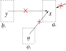
Figure 4: A portrait of $G_{{\stackrel{{\scriptstyle\wedge}}{{{\,\underline{h}\,}}}}.,{\stackrel{{\scriptstyle\wedge}}{{{\,\underline{a}\,}}}}.}$, alluded to in Claim 8

Claim 9

Let $I=\left[-H({\,\underline{x}\,}|{\,\underline{y}\,}),H({\,\underline{y}\,}:{\,\underline{x}\,})\right]$. For graphs of type INDEF defined in Fig.2, and for every $a\in I$, there exists a model with $H({\,\underline{y}\,}:{\stackrel{{\scriptstyle\wedge}}{{{\,\underline{x}\,}}}}.)=a$. Note that the lower endpoint of $I$ is $-H({\,\underline{x}\,}|{\,\underline{y}\,})=H({\,\underline{y}\,}:{\,\underline{x}\,})-H({\,\underline{x}\,})$.

proof:

$H({\,\underline{y}\,}:{\stackrel{{\scriptstyle\wedge}}{{{\,\underline{x}\,}}}})\leq H({\,\underline{y}\,}:{\,\underline{x}\,})$ follows immediately from Eq.(29). To prove the lower bound on $H({\,\underline{y}\,}:{\stackrel{{\scriptstyle\wedge}}{{{\,\underline{x}\,}}}})$, note that

$$P(y|{\stackrel{{\scriptstyle\wedge}}{{x}}})=\sum_{u}P(y|x,u)P(u)\geq\sum_{u}P(y|x,u)P(x|u)P(u)=P(x,y)\;.$$ (34)

Hence

$$H({\,\underline{y}\,}:{\stackrel{{\scriptstyle\wedge}}{{{\,\underline{x}\,}}}})=\left\langle\ln(\frac{P(y|{\stackrel{{\scriptstyle\wedge}}{{x}}})}{P(y)})\right\rangle_{x,y}\geq\left\langle\ln P(x|y)\right\rangle_{x,y}=-H({\,\underline{x}\,}|{\,\underline{y}\,})\;$$ (35)

Next we give a model that achieves the left endpoint of the interval $I$, and another that achieves the right one.

If for all $x,y,u$, one has $P(x|u)=P(x)$ and $P(y|x,u)=P(y|x)$, then the arrows between ${\,\underline{u}\,}$ and $({\,\underline{x}\,},{\,\underline{y}\,})$ can be erased, so the graph INDEF behaves just like the graph ${\,\underline{y}\,}\leftarrow{\,\underline{x}\,}$, for which $H({\,\underline{y}\,}:{\stackrel{{\scriptstyle\wedge}}{{{\,\underline{x}\,}}}})=H({\,\underline{y}\,}:{\,\underline{x}\,})$.

To get a model for which $H({\,\underline{y}\,}:{\stackrel{{\scriptstyle\wedge}}{{{\,\underline{x}\,}}}})=-H({\,\underline{x}\,}|{\,\underline{y}\,})$ let’s assume $S_{\,\underline{u}\,}=S_{\,\underline{x}\,}=S_{\,\underline{y}\,}=Z_{0,N-1}$. Let $\oplus$ denote addition mod $N$. For all $u,x,y\in Z_{0,N-1}$, let

$$\left\{\begin{array}[]{l}P(u)=\frac{1}{N}\\ P(x|u)=\delta_{x}^{u}\\ P(y|x,u)=\delta_{y}^{x\oplus u}\end{array}\right.\;.$$ (36)

Then

$$P(x,y)=\frac{1}{N}\sum_{u}\delta_{y}^{x\oplus u}\delta_{x}^{u}=\frac{\delta_{y}^{0}}{N}\;$$ (37)

and

$$P(y|{\stackrel{{\scriptstyle\wedge}}{{x}}})=\frac{1}{N}\sum_{u}\delta_{y}^{x\oplus u}=\frac{1}{N}\;.$$ (38)

Hence,

$$H({\,\underline{y}\,}:{\stackrel{{\scriptstyle\wedge}}{{{\,\underline{x}\,}}}}) = \sum_{x,y}P(x,y)\ln\frac{P(y|{\stackrel{{\scriptstyle\wedge}}{{x}}})}{P(y)}$$ (39a)

$$= \sum_{x,y}\frac{\delta_{y}^{0}}{N}\ln\frac{\frac{1}{N}}{\delta_{y}^{0}}$$ (39b)

$$= -\ln N\;$$ (39c)

and

$$-H({\,\underline{x}\,}|{\,\underline{y}\,}) = \sum_{x,y}P(x,y)\ln P(x|y)$$ (40a)

$$= \sum_{x,y}\frac{\delta_{y}^{0}}{N}\ln\frac{\frac{1}{N}\delta_{y}^{0}}{\delta_{y}^{0}}$$ (40b)

$$= -\ln N\;.$$ (40c)

QED

Eq.(41) summarizes in tabular form the results of the last 3 claims.

$$\begin{array}[]{c||c|c|c|c}\hline\cr\begin{array}[]{c}\mbox{graph}\\ \mbox{set}\end{array}\downarrow\setminus H({\,\underline{y}\,}:{\stackrel{{\scriptstyle\wedge}}{{{\,\underline{x}\,}}}})\rightarrow&[-H({\,\underline{x}\,}|{\,\underline{y}\,}),0)&0&(0,H({\,\underline{y}\,}:{\,\underline{x}\,}))&H({\,\underline{y}\,}:{\,\underline{x}\,})\\ \hline\cr\hline\cr POS&&&&\checkmark\\ \hline\cr ZERO&&\checkmark&&\\ \hline\cr INDEF&\checkmark&\checkmark&\checkmark&\checkmark\\ \hline\cr\end{array}\;$$ (41)

Claim 10

If ${\,\underline{v}\,}.=({\,\underline{y}\,},{\,\underline{x}\,})$ and ${\,\underline{u}\,}.={\,\underline{u}\,}$, then $P(y|{\stackrel{{\scriptstyle\wedge}}{{x}}})$ is identifiable (resp., not identifiable) for the graphs POS and ZERO (resp., INDEF)

proof:

In the proof of Claim 7 (resp., Claim 8), we showed that $P(y|{\stackrel{{\scriptstyle\wedge}}{{x}}})=P(y|x)$ (resp., $P(y|{\stackrel{{\scriptstyle\wedge}}{{x}}})=P(y)$) so $P(y|{\stackrel{{\scriptstyle\wedge}}{{x}}})$ is identifiable for the POS (resp., ZERO) graphs. Claim 27 shows that $P(y|{\stackrel{{\scriptstyle\wedge}}{{x}}})$ is not identifiable for INDEF graphs.
QED

6 Semi-Markovian Net, C-components

In this section, we define what Pearl and co-workers call a semi-Markovian net and its associated c-components. Semi-Markovian nets are a special type of B-net for which the theory of identifiability is simpler than for general B-nets.

A semi-Markovian net is a B-net for which the unobserved nodes ${\,\underline{u}\,}.$ are all root nodes (i.e., have no parents). Furthermore, for each $j$, ${\,\underline{u}\,}_{j}$ has exactly two elements of the set ${\,\underline{v}\,}.$ as children. The node ${\,\underline{u}\,}_{j}$ and its two outgoing arrows will be called, as in Ref.[3], a “bi-directed arc”.

For a semi-Markovian net, Eq.(15) for the $P(x.)$ of a general B-net reduces to

$$P(x.)=\prod_{j}\left\{P(v_{j}|pa({\,\underline{v}\,}_{j}))\right\}\prod_{k}\left\{P(u_{k})\right\}\;.$$ (42)

Therefore, for a semi-Markovian net,

$$P(v.)=\left\langle\prod_{j}P(v_{j}|v.\cap pa({\,\underline{v}\,}_{j}),u.\cap pa({\,\underline{v}\,}_{j}))\right\rangle_{u.}\;.$$ (43)

Note that $v.\cap pa({\,\underline{v}\,}_{j})=pa({\,\underline{v}\,}_{j},G_{{\,\underline{v}\,}.})$.

Henceforth, given a set ${\,\underline{a}\,}.\subset{\,\underline{v}\,}.$ where ${\,\underline{v}\,}.$ are the visible nodes of graph $G$, we will use the notations

$$[{\,\underline{a}\,}.]^{c}={\,\underline{v}\,}.-{\,\underline{a}\,}.\;,$$ (44)

for the complement (in ${\,\underline{v}\,}.$) of the set ${\,\underline{a}\,}.$, and

$${P(a.|[\;]^{c\wedge})}=P(a.|[a.]^{c\wedge})=P(a.|[v.-a.]^{\wedge})\;$$ (45)

for the probability of ${\,\underline{a}\,}.$ with uprooted complement. This notation is idiosyncratic to this paper. In Ref.[3], Tian and Pearl denote ${P(a.|[\;]^{c\wedge})}$ by $Q[{\,\underline{a}\,}.]$.

By the definition of the uprooting operator,

$${P(a.|[\;]^{c\wedge})}=\left\langle\prod_{j:{\,\underline{v}\,}_{j}\in{\,\underline{a}\,}.}P(v_{j}|pa({\,\underline{v}\,}_{j},G_{{\,\underline{v}\,}.}),u.)\right\rangle_{{\,\underline{u}\,}.}\;.$$ (46)

Given any two elements ${\,\underline{v}\,}_{j_{1}}$ and ${\,\underline{v}\,}_{j_{2}}$ of ${\,\underline{v}\,}.$, we will write ${\,\underline{v}\,}_{j_{1}}\sim{\,\underline{v}\,}_{j_{1}}$ and say ${\,\underline{v}\,}_{j_{1}}$ and ${\,\underline{v}\,}_{j_{2}}$ are equivalent if there is an undirected path from ${\,\underline{v}\,}_{j_{1}}$ to ${\,\underline{v}\,}_{j_{2}}$ along arrows all of which emanate from ${\,\underline{u}\,}.$ nodes. This is an equivalence relation, and it partitions ${\,\underline{v}\,}.$ into equivalence classes. We will call such classes the c-components (connected or confounding components) of ${\,\underline{v}\,}.$ and we will denote them by ${({\,\underline{v}\,}.)_{cc\;\gamma}}$ for $\gamma=0,1,2,\ldots,N_{\,\underline{\gamma}\,}-1$. For each $\gamma$, we can also find a set $({\,\underline{u}\,}.)_{\gamma}\subset{\,\underline{u}\,}.$ such that $({\,\underline{u}\,}.)_{\gamma}={\,\underline{u}\,}.\cap{\,\underline{pa}\,}({({\,\underline{v}\,}.)_{cc\;\gamma}})$. Just like the sets $\{{({\,\underline{v}\,}.)_{cc\;\gamma}}\}_{\forall\gamma}$ give a disjoint partition of ${\,\underline{v}\,}.$, the sets $\{({\,\underline{u}\,}.)_{\gamma}\}_{\forall\gamma}$ give a disjoint partition of ${\,\underline{u}\,}.$. Thus, we can write

$${\,\underline{v}\,}.=\bigcup_{\gamma}{({\,\underline{v}\,}.)_{cc\;\gamma}}\;,\;\;{\,\underline{u}\,}.=\bigcup_{\gamma}({\,\underline{u}\,}.)_{\gamma}\;$$ (47a)

It is easy to see that $P(v.)$ can be expressed as follows, as a product of factors labeled by the c-component label $\gamma$:

$$P(v.)=\prod_{\gamma}{P({(v.)_{cc\;\gamma}}|[\;]^{c\wedge})}\;,$$ (47b)

where

$${P({(v.)_{cc\;\gamma}}|[\;]^{c\wedge})}=\left\langle\prod_{j:{\,\underline{v}\,}_{j}\in{({\,\underline{v}\,}.)_{cc\;\gamma}}}P(v_{j}|pa({\,\underline{v}\,}_{j},G_{{\,\underline{v}\,}.}),(u.)_{\gamma})\right\rangle_{(u.)_{\gamma}}\;.$$ (47c)

We end this section by proving various properties of semi-Markovian nets that are useful in the theory of identifiability.

Claim 11

(Lemma 1 in Ref.[3]) Consider a semi-Markovian net so that Eqs.(47) apply. Suppose $\{{\,\underline{v}\,}\left\langle j\right\rangle\}_{\forall j}$ is a topological ordering of the set ${\,\underline{v}\,}.$ in the graph $G$. Let ${\,\underline{v}\,}.$ have the c-component decomposition

$${\,\underline{v}\,}.=\bigcup_{\gamma}{({\,\underline{v}\,}.)_{cc\;\gamma}}\;.$$ (48)

Then

$$P(v.)=\prod_{\gamma}{P({(v.)_{cc\;\gamma}}|[\;]^{c\wedge})}\;$$ (49)

where

$${P({(v.)_{cc\;\gamma}}|[\;]^{c\wedge})}=\prod_{j:{\,\underline{v}\,}\left\langle j\right\rangle\in{({\,\underline{v}\,}.)_{cc\;\gamma}}}P(v\left\langle j\right\rangle|v\left\langle<j\right\rangle)\;.$$ (50)

proof:

Since the ${\,\underline{u}\,}.$ are all root nodes, a top-ord of $G$ is given by

$${\,\underline{v}\,}\left\langle|{\,\underline{v}\,}.|\right\rangle\leftarrow\ldots\leftarrow{\,\underline{v}\,}\left\langle 2\right\rangle\leftarrow{\,\underline{v}\,}\left\langle 1\right\rangle\leftarrow{\,\underline{u}\,}\left\langle|{\,\underline{u}\,}.|\right\rangle\leftarrow\ldots\leftarrow{\,\underline{u}\,}\left\langle 2\right\rangle\leftarrow{\,\underline{u}\,}\left\langle 1\right\rangle\;.$$ (51)

Now remember that if ${\,\underline{x}\,}.=({\,\underline{x}\,}_{1},{\,\underline{x}\,}_{2},\ldots{\,\underline{x}\,}_{N})$ are the nodes of the graph, and $\{{\,\underline{x}\,}\left\langle j\right\rangle\}_{\forall j}$ is a top-ord of them, then one can use the chain rule with conditioning on past nodes or one can use it with conditioning on future nodes:

$$P(x.) = \prod_{j=1}^{N}P({\,\underline{x}\,}_{j}|{\,\underline{x}\,}\left\langle<j\right\rangle)$$ (52a)

$$= \prod_{j=1}^{N}P({\,\underline{x}\,}_{j}|{\,\underline{x}\,}\left\langle>j\right\rangle)\;$$ (52b)

where ${\,\underline{x}\,}\left\langle<1\right\rangle={\,\underline{x}\,}\left\langle>N\right\rangle=1$. If we use the chain rule which conditions on the future nodes, then we get

$$P(x.)=P(u.|v.)\prod_{j=1}^{|{\,\underline{v}\,}.|}P(v\left\langle j\right\rangle|v\left\langle>j\right\rangle)\;.$$ (53)

Summing over $u.$ then gives

$$P(v.) = \prod_{j=1}^{|{\,\underline{v}\,}.|}P(v\left\langle j\right\rangle|v\left\langle>j\right\rangle)$$ (54a)

$$= \prod_{j=1}^{|{\,\underline{v}\,}.|}P(v\left\langle j\right\rangle|v\left\langle<j\right\rangle)\;.$$ (54b)

Eq.(50) follows by applying $\delta_{[{\,\underline{v}\,}.-{({\,\underline{v}\,}.)_{cc\;\gamma}}]^{\wedge}}$ to both sides of Eq.(54b).
QED

Claim 12

(Lemma 4 in Ref.[3]) Consider a semi-Markovian net so that Eqs.(47) apply. Suppose ${\,\underline{h}\,}.\subset{\,\underline{v}\,}.$ and $\{{\,\underline{h}\,}\left\langle j\right\rangle\}_{\forall j}$ is a topological ordering of the set ${\,\underline{h}\,}.$ in the graph $G$. Let ${\,\underline{h}\,}.$ have the c-component decomposition

$${\,\underline{h}\,}.=\bigcup_{\gamma}{({\,\underline{h}\,}.)_{cc\;\gamma}}\;.$$ (55)

Then

$${P(h.|[\;]^{c\wedge})}=\prod_{\gamma}{P({(h.)_{cc\;\gamma}}|[\;]^{c\wedge})}\;$$ (56)

where

$${P({(h.)_{cc\;\gamma}}|[\;]^{c\wedge})}=\prod_{j:{\,\underline{h}\,}\left\langle j\right\rangle\in{({\,\underline{h}\,}.)_{cc\;\gamma}}}P(h\left\langle j\right\rangle|h\left\langle<j\right\rangle,h.^{c\wedge})\;$$ (57)

proof:

Note that this claim reduces to Claim 11. when ${\,\underline{h}\,}.={\,\underline{v}\,}.$ because ${\,\underline{v}\,}.^{c}=\emptyset$. The proof of this claim is very similar to the proof of Claim 11.
QED

Claim 13

(Lemma 3 in Ref.[3]) Consider a semi-Markovian net so that Eqs.(47) apply. Suppose ${\,\underline{a}\,}.\subset{\,\underline{c}\,}.\subset{\,\underline{v}\,}.$ and ${\,\underline{a}\,}.$ is ancestral in $G_{{\,\underline{c}\,}.}$. Then

$$\underbrace{\sum_{c.-a.}{P(c.|[\;]^{c\wedge})}}_{=P(a.|c.^{c\wedge})}={P(a.|[\;]^{c\wedge})}\;.$$ (58)

In particular, if ${\,\underline{c}\,}.={\,\underline{v}\,}.$, then

$$\underbrace{\sum_{v.-a.}P(v.)}_{=P(a.)}={P(a.|[\;]^{c\wedge})}\;.$$ (59)

proof:

Just note that

$$P(a.|c.^{c\wedge}) = \sum_{c.-a.}\left\langle\prod_{j:{\,\underline{v}\,}_{j}\in{\,\underline{c}\,}.-{\,\underline{a}\,}.}\left\{P(v_{j}|pa({\,\underline{v}\,}_{j}))\right\}\prod_{j:{\,\underline{v}\,}_{j}\in{\,\underline{a}\,}.}\{P(v_{j}|\underbrace{pa({\,\underline{v}\,}_{j})}_{\subset{\,\underline{a}\,}.\cup{\,\underline{u}\,}.})\}\right\rangle_{u.}$$ (60a)

$$= \left\langle\prod_{j:{\,\underline{v}\,}_{j}\in{\,\underline{a}\,}.}P(v_{j}|pa({\,\underline{v}\,}_{j}))\right\rangle_{u.}$$ (60b)

$$= {P(a.|[\;]^{c\wedge})}\;.$$ (60c)

An alternative proof, based on the do-calculus rules, is as follows. We want to show that

$$P(a.|c.^{c\wedge})=\underbrace{{P(a.|[\;]^{c\wedge})}}_{P(a.|(c.-a.)^{\wedge},c.^{c\wedge})}\;.$$ (61)

See Ref.[8] where the 3 Rules of Judea Pearl’s do-calculus are stated. Using the notation there, let ${\,\underline{b}\,}.={\,\underline{a}\,}.$, ${\,\underline{A}\,}.={\,\underline{c}\,}.-{\,\underline{a}\,}.$, ${\,\underline{h}\,}.={\,\underline{v}\,}.-{\,\underline{c}\,}.$, ${\,\underline{i}\,}.=\emptyset$, ${\,\underline{o}\,}.={\,\underline{u}\,}.$. Note that ${\,\underline{A}\,}.^{-}={\,\underline{A}\,}.-{\,\underline{an}\,}({\,\underline{i}\,}.,G_{{\stackrel{{\scriptstyle\wedge}}{{{\,\underline{h}\,}}}}.})={\,\underline{A}\,}.$ so $G_{{\stackrel{{\scriptstyle\wedge}}{{{\,\underline{h}\,}}}}.,({\,\underline{A}\,}.^{-})^{\wedge}}=G_{{\stackrel{{\scriptstyle\wedge}}{{{\,\underline{h}\,}}}}.,{\stackrel{{\scriptstyle\wedge}}{{{\,\underline{A}\,}}}}.}$. Fig.5 portrays $G_{{\stackrel{{\scriptstyle\wedge}}{{{\,\underline{h}\,}}}}.,{\stackrel{{\scriptstyle\wedge}}{{{\,\underline{A}\,}}}}.}$. Apply Rule 3 to that figure.
QED

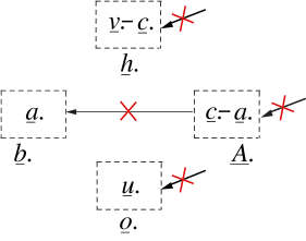
Figure 5: A portrait of $G_{{\stackrel{{\scriptstyle\wedge}}{{{\,\underline{h}\,}}}}.,{\stackrel{{\scriptstyle\wedge}}{{{\,\underline{A}\,}}}}.}$ alluded to in Claim 13.

7 $P(s.|{\stackrel{{\scriptstyle\wedge}}{{t}}}.)$ when ${\,\underline{t}\,}.={\,\underline{t}\,}$ is a singleton

In Section 7.1, we will give an algorithm for $P_{{\,\underline{v}\,}.}$ expressing $P(s.|{\stackrel{{\scriptstyle\wedge}}{{t}}}.)$ where ${\,\underline{t}\,}.={\,\underline{t}\,}$ is a singleton. In section 7.2, we will prove that the algorithm fails iff $P(s.|{\stackrel{{\scriptstyle\wedge}}{{t}}})$ is not identifiable in $G$.

Appendices A and B contain several examples of graphs and of quantities $P(s.|{\stackrel{{\scriptstyle\wedge}}{{t}}}.)$ in those graphs, with ${\,\underline{t}\,}.={\,\underline{t}\,}$ singleton. In the examples of Appendix A, we show that $P(s.|{\stackrel{{\scriptstyle\wedge}}{{t}}})$ is identifiable and we proceed to $P_{{\,\underline{v}\,}.}$ express it, using the algorithm given below. In the examples of Appendix B, we show that $P(s.|{\stackrel{{\scriptstyle\wedge}}{{t}}})$ is not identifiable by giving two different models of the graph $G$ that have the same $P_{{\,\underline{v}\,}.}$ but different $P(s.|{\stackrel{{\scriptstyle\wedge}}{{t}}})$.

7.1 Algorithm for $P_{{\,\underline{v}\,}.}$ expressing $P(s.|{\stackrel{{\scriptstyle\wedge}}{{t}}})$

In this section, we will give an algorithm for $P_{{\,\underline{v}\,}.}$ expressing $P(s.|{\stackrel{{\scriptstyle\wedge}}{{t}}}.)$ where ${\,\underline{t}\,}.={\,\underline{t}\,}$ is a singleton.

Suppose ${\,\underline{d}\,}.$ is the ancestral set of ${\,\underline{s}\,}.$ in $G_{{\,\underline{v}\,}.-{\,\underline{t}\,}}$ so

$${\,\underline{d}\,}.={\,\underline{\overline{an}}\,}({\,\underline{s}\,}.,G_{{\,\underline{v}\,}.-{\,\underline{t}\,}})\;,$$ (62)

and let

$${\,\underline{r}\,}.={\,\underline{v}\,}.-{\,\underline{d}\,}.\;.$$ (63)

Note that

$$P(s.|{\stackrel{{\scriptstyle\wedge}}{{t}}}) = P(s.|[(v.-t)-d.]^{\wedge},{\stackrel{{\scriptstyle\wedge}}{{t}}})$$ (64a)

$$= P(s.|[v.-d.]^{\wedge})$$ (64b)

$$= P(s.|d.^{c\wedge})\;,$$ (64c)

where Eq.(64a) follows from Claim 13.

Let ${\,\underline{v}\,}.=\bigcup_{\gamma}{({\,\underline{v}\,}.)_{cc\;\gamma}}$ be the c-component decomposition of ${\,\underline{v}\,}.$ in $G_{{\,\underline{v}\,}.}$. For each $\gamma$, let

$$({\,\underline{d}\,}.)_{\gamma}={\,\underline{d}\,}.\cap{({\,\underline{v}\,}.)_{cc\;\gamma}}\;$$ (65)

and

$$({\,\underline{r}\,}.)_{\gamma}={\,\underline{r}\,}.\cap{({\,\underline{v}\,}.)_{cc\;\gamma}}={({\,\underline{v}\,}.)_{cc\;\gamma}}-({\,\underline{d}\,}.)_{\gamma}\;.$$ (66)

Note that ${\,\underline{d}\,}.=\bigcup_{\gamma}({\,\underline{d}\,}.)_{\gamma}$ and the $({\,\underline{d}\,}.)_{\gamma}$ are mutually disjoint but they are not c-components. That’s why we denote them as $({\,\underline{d}\,}.)_{\gamma}$ instead of $({\,\underline{d}\,}.)_{cc\;\gamma}$.

Claim 14

$${P(d.|[\;]^{c\wedge})}=\prod_{\gamma}{P((d.)_{\gamma}|[\;]^{c\wedge})}\;.$$ (67)

proof:

Let LHS and RHS denote the left and right hand sides of Eq.(67). Then

$$LHS = \delta_{[{\,\underline{v}\,}.-{\,\underline{d}\,}.]^{\wedge}}P(v.)$$ (68a)

$$= \delta_{[{\,\underline{v}\,}.-{\,\underline{d}\,}.]^{\wedge}}\prod_{\gamma}{P({(v.)_{cc\;\gamma}}|[\;]^{c\wedge})}$$ (68b)

$$= \prod_{\gamma}\left\{\delta_{[{({\,\underline{v}\,}.)_{cc\;\gamma}}-({\,\underline{d}\,}.)_{\gamma}]^{\wedge}}\right\}\prod_{\gamma}\left\{{P({(v.)_{cc\;\gamma}}|[\;]^{c\wedge})}\right\}$$ (68c)

$$= \prod_{\gamma}\left\{\delta_{[{({\,\underline{v}\,}.)_{cc\;\gamma}}-({\,\underline{d}\,}.)_{\gamma}]^{\wedge}}{P({(v.)_{cc\;\gamma}}|[\;]^{c\wedge})}\right\}$$ (68d)

$$= RHS\;$$ (68e)

QED

Define $\gamma_{t}$ to be the $\gamma$ such that ${\,\underline{t}\,}\in{({\,\underline{v}\,}.)_{cc\;\gamma}}$. We will also use the following shorthand notations

$${\,\underline{{\cal V}}\,}.={({\,\underline{v}\,}.)_{cc\;\gamma_{t}}}\;,\;\;{\,\underline{{\cal D}}\,}.=({\,\underline{d}\,}.)_{\gamma_{t}}\;,\;\;{\,\underline{{\cal R}}\,}.=({\,\underline{r}\,}.)_{\gamma_{t}}={\,\underline{{\cal V}}\,}.-{\,\underline{{\cal D}}\,}.\;$$ (69)

Claim 15

For all $\gamma\neq\gamma_{t}$,

$${P((d.)_{\gamma}|[\;]^{c\wedge})}=P((d.)_{\gamma}|{(v.)_{cc\;\gamma}}^{c\wedge})\;.$$ (70)

proof:

We want to show that

$$\underbrace{P((d.)_{\gamma}|(r.)_{\gamma}^{\wedge},{(v.)_{cc\;\gamma}}^{c\wedge})}_{={P((d.)_{\gamma}|[\;]^{c\wedge})}}=P((d.)_{\gamma}|{(v.)_{cc\;\gamma}}^{c\wedge})\;.$$ (71)

See Ref.[8] where the 3 Rules of Judea Pearl’s do-calculus are stated. Using the notation there, let ${\,\underline{b}\,}.=({\,\underline{d}\,}.)_{\gamma}$, ${\,\underline{a}\,}.=({\,\underline{r}\,}.)_{\gamma}$, ${\,\underline{h}\,}.={({\,\underline{v}\,}.)_{cc\;\gamma}}^{c}$, ${\,\underline{i}\,}.=\emptyset$,, ${\,\underline{o}\,}.={\,\underline{u}\,}.$. Note that ${\,\underline{a}\,}.^{-}={\,\underline{a}\,}.-{\,\underline{an}\,}({\,\underline{i}\,}.,G_{{\stackrel{{\scriptstyle\wedge}}{{{\,\underline{h}\,}}}}.})={\,\underline{a}\,}.$ so $G_{{\stackrel{{\scriptstyle\wedge}}{{{\,\underline{h}\,}}}}.,({\,\underline{a}\,}.^{-})^{\wedge}}=G_{{\stackrel{{\scriptstyle\wedge}}{{{\,\underline{h}\,}}}}.,{\stackrel{{\scriptstyle\wedge}}{{{\,\underline{a}\,}}}}.}$. Fig.6 portrays $G_{{\stackrel{{\scriptstyle\wedge}}{{{\,\underline{h}\,}}}}.,{\stackrel{{\scriptstyle\wedge}}{{{\,\underline{a}\,}}}}.}$. Apply Rule 3 to that figure.
QED

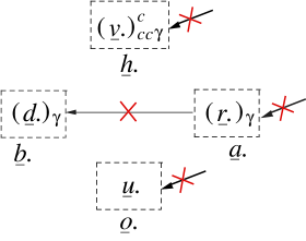
Figure 6: A portrait of $G_{{\stackrel{{\scriptstyle\wedge}}{{{\,\underline{h}\,}}}}.,{\stackrel{{\scriptstyle\wedge}}{{{\,\underline{a}\,}}}}.}$ alluded to in Claim 15.

Claim 16

$${P({\cal D}.|[\;]^{c\wedge})}=P({\cal D}.|{\cal V}.^{c\wedge},{\stackrel{{\scriptstyle\wedge}}{{t}}})\;.$$ (72)

proof:

We want to show that

$$\underbrace{P({\cal D}.|[{\cal R}.-t]^{\wedge},{\cal V}.^{c\wedge},{\stackrel{{\scriptstyle\wedge}}{{t}}})}_{={P({\cal D}.|[\;]^{c\wedge})}}=P({\cal D}.|{\cal V}.^{c\wedge},{\stackrel{{\scriptstyle\wedge}}{{t}}})\;.$$ (73)

See Ref.[8] where the 3 Rules of Judea Pearl’s do-calculus are stated. Using the notation there, let ${\,\underline{b}\,}.={\,\underline{{\cal D}}\,}.$, ${\,\underline{a}\,}.={\,\underline{{\cal R}}\,}.-{\,\underline{t}\,}$, ${\,\underline{h}\,}.=({\,\underline{{\cal V}}\,}.^{c},{\,\underline{t}\,})$, ${\,\underline{i}\,}.=\emptyset$,, ${\,\underline{o}\,}.={\,\underline{u}\,}.$. Note that ${\,\underline{a}\,}.^{-}={\,\underline{a}\,}.-{\,\underline{an}\,}({\,\underline{i}\,}.,G_{{\stackrel{{\scriptstyle\wedge}}{{{\,\underline{h}\,}}}}.})={\,\underline{a}\,}.$ so $G_{{\stackrel{{\scriptstyle\wedge}}{{{\,\underline{h}\,}}}}.,({\,\underline{a}\,}.^{-})^{\wedge}}=G_{{\stackrel{{\scriptstyle\wedge}}{{{\,\underline{h}\,}}}}.,{\stackrel{{\scriptstyle\wedge}}{{{\,\underline{a}\,}}}}.}$. Fig.7 portrays $G_{{\stackrel{{\scriptstyle\wedge}}{{{\,\underline{h}\,}}}}.,{\stackrel{{\scriptstyle\wedge}}{{{\,\underline{a}\,}}}}.}$. Apply Rule 3 to that figure.
QED

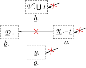
Figure 7: A portrait of $G_{{\stackrel{{\scriptstyle\wedge}}{{{\,\underline{h}\,}}}}.,{\stackrel{{\scriptstyle\wedge}}{{{\,\underline{a}\,}}}}.}$ alluded to in Claim 16.

Now we can combine Eqs. (64c), (67), (70), (72) to get

$$P(s.|{\stackrel{{\scriptstyle\wedge}}{{t}}})=\sum_{d.-s.}P({\cal D}.|{\cal V}.^{c\wedge},{\stackrel{{\scriptstyle\wedge}}{{t}}})\prod_{\gamma\neq\gamma_{t}}P((d.)_{\gamma}|\;{(v.)_{cc\;\gamma}}^{c\wedge})\;.$$ (74)

Eq.(74) is reminiscent of cutting a pie. Fig.8 explains this analogy further. In this figure, ${\,\underline{s}\,}.$, ${\,\underline{d}\,}.$ and ${\,\underline{v}\,}.$ are circular regions nested this way: ${\,\underline{s}\,}.\subset{\,\underline{d}\,}.\subset{\,\underline{v}\,}.$. Let $0,1,2,\ldots,6$ denote points on the pie, and let $(0,1,2)$ be the pie slice with corners $0,1,2$. Then ${\cal D}.=(0,1,2)$, ${\cal V}.=(0,4,5)$. Note that ${\,\underline{t}\,}\in{\cal V}.$. For some $\gamma$ different from $\gamma_{t}$, $({\,\underline{d}\,}.)_{\gamma}=(0,2,3)$ and ${({\,\underline{v}\,}.)_{cc\;\gamma}}=(0,5,6)$.

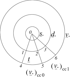
Figure 8: Pie-cutting analogy for Eq.(74).

Eq.(74) suggests the following iterative algorithm. To $P_{{\,\underline{v}\,}.}$ express $P(s.|{\stackrel{{\scriptstyle\wedge}}{{t}}})$, call ${\tt PV\_EXPRESS\_ONE}({\,\underline{s}\,}.,{\,\underline{t}\,},{\,\underline{v}\,}.)$, where

Subroutine ${\tt PV\_EXPRESS\_ONE}({\,\underline{\sigma}\,}.,{\,\underline{t}\,},{\,\underline{\beta}\,}.)$ {
	inputs:$({\,\underline{\sigma}\,}.,{\,\underline{t}\,},{\,\underline{\beta}\,}.)$, where must have ${\,\underline{\sigma}\,}.\cap{\,\underline{t}\,}=\emptyset$ and ${\,\underline{\sigma}\,}.\cup{\,\underline{t}\,}\subset{\,\underline{\beta}\,}.\subset{\,\underline{v}\,}.$
	Set continue_flag = true.
	Do while (continue_flag == true) {
		Find c-components $\{{({\,\underline{\beta}\,}.)_{cc\;\gamma}}\}_{\forall\gamma}$ of ${\,\underline{\beta}\,}.$ in $G_{{\,\underline{\beta}\,}.}$, ${\,\underline{\beta}\,}.=\bigcup_{\gamma}{({\,\underline{\beta}\,}.)_{cc\;\gamma}}$
		Find ${\,\underline{d}\,}.=\overline{\underline{an}}({\,\underline{\sigma}\,}.,G_{{\,\underline{\beta}\,}.-{\,\underline{t}\,}})$
		For all $\gamma$ { Set $({\,\underline{d}\,}.)_{\gamma}={({\,\underline{v}\,}.)_{cc\;\gamma}}\cap{\,\underline{d}\,}.\}$
		Let $\gamma_{t}$ be $\gamma$ such that ${\,\underline{t}\,}\in({\,\underline{d}\,}.)_{\gamma}$.
		Set ${\,\underline{{\cal D}}\,}.=({\,\underline{d}\,}.)_{\gamma_{t}}$ and ${\,\underline{{\cal V}}\,}.={({\,\underline{v}\,}.)_{cc\;\gamma_{t}}}$.
		Store expression $P(\sigma.|{\stackrel{{\scriptstyle\wedge}}{{t}}})=\sum_{d.-\sigma.}P({\cal D}.|{\cal V}.^{c\wedge},{\stackrel{{\scriptstyle\wedge}}{{t}}})\prod_{\gamma\neq\gamma_{t}}P((d.)_{\gamma}|\;{(v.)_{cc\;\gamma}}^{c\wedge})$
		For all $\gamma\neq\gamma_{t}$ { Express $P((d.)_{\gamma}|\;{(\beta.)_{cc\;\gamma}}^{c\wedge})$ without hats via Claim 12 }
		Apply do-calculus Rules 2 and 3 to $P({\cal D}.|({\cal V}_{.})^{c\wedge},{\stackrel{{\scriptstyle\wedge}}{{t}}})$ to see if ${\stackrel{{\scriptstyle\wedge}}{{t}}}=\tau\in\{1,t\}$
		If Rule 2 or 3 succeeds {
			Express $P({\cal D}.|({\cal V}.)^{c\wedge},\tau)$ without hats via Claim 12.
			Set continue_flag = false
		} else {
			Prune graph: Replace graph $G_{{\,\underline{\beta}\,}.}$ by $G_{{\,\underline{\beta}\,}.^{-}}$, where ${\,\underline{\beta}\,}.^{-}=\overline{{\,\underline{an}\,}}({\,\underline{\sigma}\,}.\cup{\,\underline{t}\,},G_{{\,\underline{\beta}\,}.})$.
			Set ${\,\underline{\beta}\,}.\leftarrow{\,\underline{\beta}\,}.^{-}$
			If ${\,\underline{{\cal D}.}\,}$ is a c-component of $G_{{\,\underline{\beta}\,}.}$ {
				Return FAIL message
				Exit program
			}
		}
	}
	Do loop must store information with each step.
	Collect information from each step of the sequence
	to assemble expression without hats
	for the $P(s.|{\stackrel{{\scriptstyle\wedge}}{{t}}})$ considered at the beginning of the sequence.
}

Note that this algorithm “prunes” the graph before looping back again. Pruning the graph is justified by virtue of Claim 2. It is a convenient step that gets rid of superfluous nodes. It also turns out to be a necessary step. As illustrated by the example of Section A.6, the algorithm ${\tt PV\_EXPRESS\_ONE}()$ may fail if this step is not performed.

The algorithm ${\tt PV\_EXPRESS\_ONE()}$ applies Eq.74 once in each loop step. The first application uses $({\,\underline{s}\,}.^{(1)},{\,\underline{v}\,}.^{(1)})=({\,\underline{s}\,}.,{\,\underline{v}\,}.)$ and generates $({\,\underline{{\cal D}}\,}.,{\,\underline{{\cal V}}\,}.)$ which becomes $({\,\underline{s}\,}.^{(2)},{\,\underline{v}\,}.^{(2)})$ for the next step. The algorithm thus generates a sequence $\{({\,\underline{s}\,}.^{(j)},{\,\underline{v}\,}.^{(j)})\}_{j=1}^{N}$. The sequence terminates when ${\,\underline{s}\,}.^{(N)}$ is a c-component of the current graph.

7.2 Necessary and Sufficient Conditions for Identifiability of $P(s.|{\stackrel{{\scriptstyle\wedge}}{{t}}})$

In this section, we will prove that the algorithm given in Section 7.2 fails iff $P(s.|{\stackrel{{\scriptstyle\wedge}}{{t}}})$ is not identifiable in $G$.

Claim 17

If $P({\cal D}.|{\cal V}.^{c\wedge},{\stackrel{{\scriptstyle\wedge}}{{t}}})=P({\cal D}.|{\cal V}.^{c\wedge},\tau)$ where $\tau\in\{1,t\}$, then $H({\,\underline{s}\,}.:{\stackrel{{\scriptstyle\wedge}}{{{\,\underline{t}\,}}}})\geq 0$.

proof:

Assume the premise of the claim. Combine that with Eqs. (47b) and (74) to get

$$P(s.:{\stackrel{{\scriptstyle\wedge}}{{t}}}) = \frac{1}{P(s.)}\sum_{d.-s.}P({\cal D}.|{\cal V}.^{c\wedge},\tau)\prod_{\gamma\neq\gamma_{t}}P((d.)_{\gamma}|{(v.)_{cc\;\gamma}}^{c\wedge})$$ (75a)

$$= \frac{1}{P(s.)}\sum_{d.-s.}P(v.)\frac{P({\cal D}.|{\cal V}.^{c\wedge},\tau)}{P({\cal V}.|{\cal V}.^{c\wedge})}\prod_{\gamma\neq\gamma_{t}}\left\{\frac{P((d.)_{\gamma}|{(v.)_{cc\;\gamma}}^{c\wedge})}{P((v.)_{\gamma}|{(v.)_{cc\;\gamma}}^{c\wedge})}\right\}\;.$$ (75b)

Next note that

$$\frac{P({\cal D}.|{\cal V}.^{c\wedge},\tau)}{P({\cal V}.|{\cal V}.^{c\wedge})}=\frac{1}{P(\tau|{\cal V}.^{c\wedge})P({\cal R}.-\tau|{\cal V}.^{c\wedge},{\cal D}.,\tau)}\;,$$ (76)

and

$$\prod_{\gamma\neq\gamma_{t}}\left\{\frac{P((d.)_{\gamma}|{(v.)_{cc\;\gamma}}^{c\wedge})}{P((v.)_{\gamma}|{(v.)_{cc\;\gamma}}^{c\wedge})}\right\}=\frac{1}{\prod_{\gamma\neq\gamma_{t}}P((r.)_{\gamma}|{(v.)_{cc\;\gamma}}^{c\wedge},(d.)_{\gamma})}\;.$$ (77)

Defining a conditional probability distribution $Q(r.|v.-r.)$ by

$$Q(r.|v.-r.)=P(\tau|{\cal V}.^{c\wedge})P({\cal R}.-\tau|{\cal V}.^{c\wedge},{\cal D}.,\tau)\prod_{\gamma\neq\gamma_{t}}P((r.)_{\gamma}|{(v.)_{cc\;\gamma}}^{c\wedge},(d.)_{\gamma})\;$$ (78)

allows us to write Eq.(75b) more succinctly as

$$P(s.:{\stackrel{{\scriptstyle\wedge}}{{t}}})=\sum_{d.-s.}\frac{P(v.)}{P(s.)Q(r.|v.-r.)}\;.$$ (79)

Define

$$Q(v.)=P(d.-s.|r.\cup s.)P(s.)Q(r.|v.-r.)\;.$$ (80)

Now note that

$$H({\,\underline{s}\,}.:{\stackrel{{\scriptstyle\wedge}}{{{\,\underline{t}\,}}}}) = \left\langle\ln P(s.:{\stackrel{{\scriptstyle\wedge}}{{t}}})\right\rangle_{s.,t}$$ (81a)

$$= \left\langle\ln P(s.:{\stackrel{{\scriptstyle\wedge}}{{t}}})\right\rangle_{s.,t,r.-t}$$ (81b)

$$= \left\langle\ln(\sum_{d.-s.}\frac{P(d.-s.|r.\cup s.)}{P(d.-s.|r.\cup s.)}\frac{P(v.)}{P(s.)Q(r.|v.-r.)})\right\rangle_{s.\cup r.}$$ (81c)

$$= \left\langle\ln(\sum_{d.-s.}P(d.-s.|r.\cup s.)\frac{P(v.)}{Q(v.)})\right\rangle_{s.\cup r.}$$ (81d)

$$\geq \left\langle\ln(\frac{P(v.)}{Q(v.)})\right\rangle_{P(v.)}$$ (81e)

$$= D(P(v.)//Q(v.))_{\forall v.}\geq 0\;.$$ (81f)

Eq.(81b) follows because the quantity being averaged, $P(s.|{\stackrel{{\scriptstyle\wedge}}{{t}}})$, depends only on $s.$ and $t$. Since it is independent of $r.-t$, we may do a weighted average over $r.-t$ also without changing the final average. Inequality Eq.(81e) follows from the concavity of the $\ln(\cdot)$ function. Indeed, $\ln(x)$ is a concave function over $x\in{\mathbb{R}}^{\geq 0}$ so if $P(a)$ is a probability distribution over $S_{\,\underline{a}\,}$ and $f(a)\geq 0$ for all $a\in S_{\,\underline{a}\,}$, then

$$\ln\left(\sum_{a}P(a)f(a)\right)\geq\sum_{a}P(a)\ln\left(f(a)\right)\;.$$ (82)

QED

Next we give one of the most important claims of this paper. The claim might even come close to the exalted level of being called a theorem. It gives two separate conditions, one “graphical”, and one “informational”, such that either of them alone is necessary and sufficient for $P(s.|{\stackrel{{\scriptstyle\wedge}}{{t}}})$ to be identifiable in $G$.

Claim 18

For any graph $G$, the following are equivalent:

(ID)

$P(s.|{\stackrel{{\scriptstyle\wedge}}{{t}}})$ is identifiable in $G$.

(GR)

$P(s.^{(N)}|(v.^{(N)})^{c\wedge},{\stackrel{{\scriptstyle\wedge}}{{t}}})=P(s.^{(N)}|(v.^{(N)})^{c\wedge},\tau)$ where $\tau\in\{1,t\}$. $({\,\underline{s}\,}.^{(N)},{\,\underline{v}\,}.^{(N)})$ is the last term in the sequence $\{({\,\underline{s}\,}.^{(j)},{\,\underline{v}\,}.^{(j)})\}_{j=1}^{N}$ generated by the algorithm PV_EXPRESS_ONE().

(H+)

$H({\,\underline{s}\,}.:{\stackrel{{\scriptstyle\wedge}}{{{\,\underline{t}\,}}}})\geq 0$ for all models of $G$.

proof:

(GR$\implies$ ID)

Assume GR. Then after applying Eq.(74) multiple times, we get a product of $P_{{\,\underline{v}\,}.}$ expressible probabilities times $P(s.^{(N)}|(v.^{(N)})^{c\wedge},{\stackrel{{\scriptstyle\wedge}}{{t}}})$. The latter is itself equal to $P(s.^{(N)}|(v.^{(N)})^{c\wedge},\tau)$ by GR. Thus ID is true.

(GR$\implies$ H+)

This follows from Claim 17.

(not(GR)$\implies$ not(ID) and not(H+))

Using the notation of Ref.[8], for $j\in\{1,2,3\}$, call $({\,\underline{b}\,}.\perp{\,\underline{a}\,}.|{\stackrel{{\scriptstyle\wedge}}{{{\,\underline{h}\,}}}}.,{\,\underline{i}\,}.)_{G_{j}}$ the “premise” of Rule $j$ . Assume not(GR). Then the Rule 2 premise and the Rule 3 premise are both false, where ${\,\underline{b}\,}.={\,\underline{s}\,}.^{(N)}$,${\,\underline{a}\,}.={\,\underline{t}\,}$, ${\,\underline{h}\,}.=({\,\underline{v}\,}.^{(N)})^{c}$, ${\,\underline{i}\,}.=\emptyset$, ${\,\underline{o}\,}.=({\,\underline{o}\,}.^{(a)},{\,\underline{o}\,}.^{(b)})$, ${\,\underline{o}\,}.^{(a)}={\,\underline{u}\,}.$, ${\,\underline{o}\,}.^{(b)}=({\,\underline{v}\,}.^{(N)}-{\,\underline{s}\,}.^{(N)}\cup{\,\underline{t}\,})$. Note that ${\,\underline{a}\,}.^{-}={\,\underline{a}\,}.-{\,\underline{an}\,}({\,\underline{i}\,}.,G_{{\stackrel{{\scriptstyle\wedge}}{{{\,\underline{h}\,}}}}.})={\,\underline{a}\,}.$ so $G_{{\stackrel{{\scriptstyle\wedge}}{{{\,\underline{h}\,}}}}.,({\,\underline{a}\,}.^{-})^{\wedge}}=G_{{\stackrel{{\scriptstyle\wedge}}{{{\,\underline{h}\,}}}}.,{\stackrel{{\scriptstyle\wedge}}{{{\,\underline{a}\,}}}}.}$. Fig.9 portrays $G_{{\stackrel{{\scriptstyle\wedge}}{{{\,\underline{h}\,}}}}.,{\stackrel{{\scriptstyle\vee}}{{{\,\underline{a}\,}}}}.}$ for Rule 2 and $G_{{\stackrel{{\scriptstyle\wedge}}{{{\,\underline{h}\,}}}}.,{\stackrel{{\scriptstyle\wedge}}{{{\,\underline{a}\,}}}}.}$ for Rule 3. Arrows with an “X R2” (resp., “X R3”) on them are banned by Rule 2 (resp., Rule 3).

Note that Fig.9 places a ban on arrows pointing from ${\,\underline{o}\,}.^{(b)}$ to ${\,\underline{b}\,}.$. This is justified because ${\,\underline{s}\,}.^{(N)}$ equals the last ${\cal D}.$ and ${\,\underline{v}\,}.^{(N)}$ equals the last ${\cal V}.$. With ${\,\underline{d}\,}.=\overline{{\,\underline{an}\,}}(\sigma.,G_{{\,\underline{\beta}\,}.-{\,\underline{t}\,}})$, we have (1) ${\,\underline{b}\,}.={\cal D}.$ is inside ${\,\underline{d}\,}.$, (2) ${\,\underline{o}\,}.^{(b)}={\cal V}.-{\cal D}.\cup{\,\underline{t}\,}$ is disjoint from ${\,\underline{d}\,}.$, and (3) ${\,\underline{d}\,}.$ is ancestral in $G_{{\,\underline{\beta}\,}.-{\,\underline{t}\,}}$.

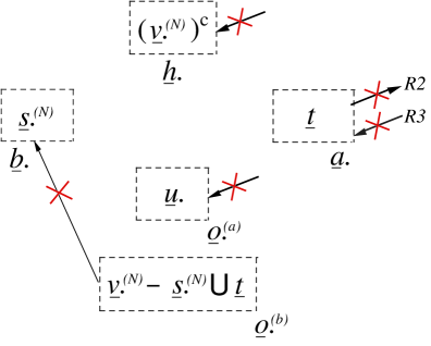
Figure 9: A portrait of $G_{{\stackrel{{\scriptstyle\wedge}}{{{\,\underline{h}\,}}}}.,{\stackrel{{\scriptstyle\vee}}{{{\,\underline{a}\,}}}}.}$ for Rule 2 and $G_{{\stackrel{{\scriptstyle\wedge}}{{{\,\underline{h}\,}}}}.,{\stackrel{{\scriptstyle\wedge}}{{{\,\underline{a}\,}}}}.}$ for Rule 3, alluded to in Claim 18. There is also a ban on arrows from ${\,\underline{o}\,}.^{(b)}$ to ${\,\underline{b}\,}.$.

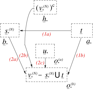
Figure 10: Possible behaviors of path $\gamma_{3}$ alluded to in Claim 18.

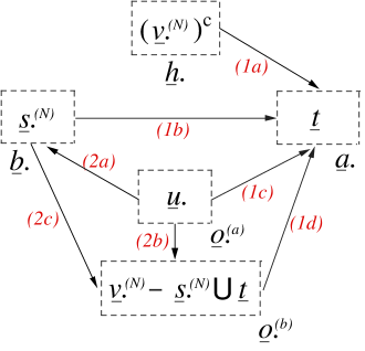
Figure 11: Possible behaviors of path $\gamma_{2}$ alluded to in Claim 18.

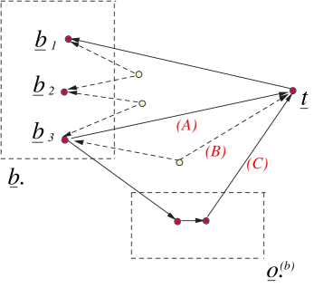
Figure 12: In Claim 18, when not(GR) is assumed, there must be a closed path of either type (A), (B) or (C). All 3 types are either standard or modified shark teeth graphs of the kind discussed in Section B.2.

Since the premise of Rule 3 is false, there must exist an undirected path $\gamma_{3}$ from ${\,\underline{a}\,}.$ to ${\,\underline{b}\,}.$ that is unblocked at fixed $({\,\underline{h}\,}.,{\,\underline{i}\,}.)$. Figure 10 illustrates possible behaviors of path $\gamma_{3}$. $\gamma_{3}$ must contain an arrow exiting node ${\,\underline{a}\,}.={\,\underline{t}\,}$. This means $\gamma_{3}$ must contain either an arrow $(1a)$ or an arrow $(1b)$. If path $\gamma_{3}$ contains arrow $(1b)$, then it must also contain at least one of the following arrows: $(2a)$ or $(2b)$ or $(2c)$. Let $\gamma_{3}\supset(1b,2a)$ mean that path $\gamma_{3}$ contains arrows $(1b)$ and $(2a)$. Thus, $\gamma_{3}$ must satisfy one of the following 4 cases.

$$\gamma_{3}\supset\left\{\begin{array}[]{ll}1a&\mbox{OK}\\ (1b,2a)&\mbox{blocked}\\ (1b,2b)&\mbox{blocked}\\ (1b,2c)&\mbox{blocked}\end{array}\right.\;.$$ (83)

As indicated, the last 3 cases are not really possible because in all 3 cases $\gamma_{3}$ would have to have a collider outside ${\,\underline{h}\,}.$, so in order for $\gamma_{3}$ to remain unblocked, that collider would have to have a descendant in ${\,\underline{h}\,}.$. But that can’t happen since there is a ban on arrows entering ${\,\underline{h}\,}.$.

Since the premise of Rule 2 is false, there must exist an undirected path $\gamma_{2}$ from ${\,\underline{a}\,}.$ to ${\,\underline{b}\,}.$ that is unblocked at fixed $({\,\underline{h}\,}.,{\,\underline{i}\,}.)$. Figure 11 illustrates possible behaviors of path $\gamma_{2}$. $\gamma_{2}$ must contain an arrow entering node ${\,\underline{a}\,}.={\,\underline{t}\,}$. This means $\gamma_{2}$ must contain one of the following arrows: $(1a),(1b),(1c)$ or $(1d)$. If path $\gamma_{2}$ contains arrow $(1c)$, then it must also contain at least one of the following arrows: $(2a)$ or $(2b)$. If path $\gamma_{2}$ contains arrow $(1d)$, then it must also contain arrow $(2c)$. Thus, $\gamma_{2}$ must satisfy one of the following 4 cases.

$$\gamma_{2}\supset\left\{\begin{array}[]{lll}1a&\mbox{blocked}&\\ 1b&\mbox{OK}&(A)\\ (1c,2a)&\mbox{OK}&(B)\\ (1c,2b)&\mbox{blocked}&\\ (1d,2c)&\mbox{OK}&(C)\end{array}\right.\;$$ (84)

As indicated, the first and fourth cases are not really possible. For the first case, $\gamma_{2}$ would have to have a non-collider inside ${\,\underline{h}\,}.$ and that would block the path. For the fourth case, $\gamma_{2}$ would have to have a collider outside ${\,\underline{h}\,}.$, so in order for $\gamma_{2}$ to remain unblocked, that collider would have to have a descendant in ${\,\underline{h}\,}.$. But that can’t happen since there is a ban on arrows entering ${\,\underline{h}\,}.$.

Fig.12 combines the OK cases for path $\gamma_{3}$ with the OK cases for path $\gamma_{2}$. Let ${\,\underline{b}\,}_{1}$ be the node where $\gamma_{3}$ first makes contact with ${\,\underline{b}\,}.$. Let ${\,\underline{b}\,}_{3}$ be the node where $\gamma_{2}$ first makes contact with ${\,\underline{b}\,}.$. There must be path between ${\,\underline{b}\,}_{1}$ and ${\,\underline{b}\,}_{3}$ that is composed of a sequence of visible nodes (for example, the visible nodes ${\,\underline{b}\,}_{1},{\,\underline{b}\,}_{2},{\,\underline{b}\,}_{3}$ in Fig.12) connected pairwise by bidirected arcs, and those visible nodes must all lie inside ${\,\underline{s}\,}.^{(N)}$. This follows because, by construction, ${\,\underline{s}\,}.^{(N)}$ is a c-component of the current graph.

Thus, the full graph $G$ must contain a subgraph, call it $G^{-}$, isomorphic to the shark teeth graph discussed in Section B.2. $G^{-}$ is not identifiable and there exists a model for it with $H({\,\underline{s}\,}.:{\stackrel{{\scriptstyle\wedge}}{{{\,\underline{t}\,}}}})<0$. Therefore, by virtue of Claims 1 and 6, $G$ is not identifiable and there exists a model for it with $H({\,\underline{s}\,}.:{\stackrel{{\scriptstyle\wedge}}{{{\,\underline{t}\,}}}})<0$.

QED

8 $P(s.|{\stackrel{{\scriptstyle\wedge}}{{t}}}.)$ when ${\,\underline{t}\,}.$ is NOT a singleton

8.1 Algorithm for $P_{{\,\underline{v}\,}.}$ expressing $P(s.|{\stackrel{{\scriptstyle\wedge}}{{t}}}.)$

In Section 8.1, we gave an algorithm called PV_EXPRESS_ONE() for $P_{{\,\underline{v}\,}.}$ expressing $P(s.|{\stackrel{{\scriptstyle\wedge}}{{t}}}.)$ when ${\,\underline{t}\,}.$ is a singleton. Below we give a recursive algorithm called PV_EXPRESS() that handles the ${\,\underline{t}\,}.$ non-singleton case by calling PV_EXPRESS_ONE() repeatedly.

To $P_{{\,\underline{v}\,}.}$ express $P(s.|{\stackrel{{\scriptstyle\wedge}}{{t}}}.)$, call ${\tt PV\_EXPRESS}({\,\underline{s}\,}.,{\,\underline{t}\,}.,{\,\underline{v}\,}.)$, where

Subroutine ${\tt PV\_EXPRESS}({\,\underline{\sigma}\,}.,{\,\underline{t}\,}.,{\,\underline{\beta}\,}.)$ {
	inputs:$({\,\underline{\sigma}\,}.,{\,\underline{t}\,}.,{\,\underline{\beta}\,}.)$, where must have ${\,\underline{\sigma}\,}.\cap{\,\underline{t}\,}.=\emptyset$ and ${\,\underline{\sigma}\,}.\cup{\,\underline{t}\,}.\subset{\,\underline{\beta}\,}.\subset{\,\underline{v}\,}.$
	Prune graph: Replace graph $G_{{\,\underline{\beta}\,}.}$ by $G_{{\,\underline{\beta}\,}.^{-}}$, where ${\,\underline{\beta}\,}.^{-}=\overline{{\,\underline{an}\,}}({\,\underline{\sigma}\,}.\cup{\,\underline{t}\,}.,G_{{\,\underline{\beta}\,}.})$.
	Set ${\,\underline{\beta}\,}.\leftarrow{\,\underline{\beta}\,}.^{-}$
	Find c-components $\{{({\,\underline{\beta}\,}.)_{cc\;\gamma}}\}_{\forall\gamma}$ of ${\,\underline{\beta}\,}.$ in $G_{{\,\underline{\beta}\,}.}$, ${\,\underline{\beta}\,}.=\bigcup_{\gamma}{({\,\underline{\beta}\,}.)_{cc\;\gamma}}$
	Find ${\,\underline{d}\,}.=\overline{\underline{an}}({\,\underline{\sigma}\,}.,G_{{\,\underline{\beta}\,}.-{\,\underline{t}\,}.})$
	For all $\gamma$ { Set $({\,\underline{d}\,}.)_{\gamma}={({\,\underline{\beta}\,}.)_{cc\;\gamma}}\cap{\,\underline{d}\,}.$ and $({\,\underline{t}\,}.)_{\gamma}={({\,\underline{\beta}\,}.)_{cc\;\gamma}}\cap{\,\underline{t}\,}.$ }
	Store expression $P(\sigma.|{\stackrel{{\scriptstyle\wedge}}{{t}}}.)=\sum_{d.-\sigma.}\prod_{\gamma}P((d.)_{\gamma}|\;{(\beta.)_{cc\;\gamma}}^{c\wedge},(t.)_{\gamma}^{\wedge})$
	For all $\gamma$ {
		If $|({\,\underline{t}\,}.)_{\gamma}|=0$ {
			Express $P((d.)_{\gamma}|\;{(\beta.)_{cc\;\gamma}}^{c\wedge})$ without hats via Claim 12
		} else if $|({\,\underline{t}\,}.)_{\gamma}|=1$ {
			Call ${\tt PV\_EXPRESS\_ONE}(({\,\underline{d}\,}.)_{\gamma},{\,\underline{t}\,},{({\,\underline{\beta}\,}.)_{cc\;\gamma}})$
		} else if $|({\,\underline{t}\,}.)_{\gamma}|>1$ {
			Call ${\tt PV\_EXPRESS}(({\,\underline{d}\,}.)_{\gamma},({\,\underline{t}\,}.)_{\gamma},{({\,\underline{\beta}\,}.)_{cc\;\gamma}})$
		}
	}
	Revisit all nodes of the recursion tree, and
	collect information from each node of tree
	to assemble expression without hats
	for the $P(s.|{\stackrel{{\scriptstyle\wedge}}{{t}}}.)$ at the root node of tree.
}

The above subroutine appears to be consistent. It appears to fail if and only if $P(s.|{\stackrel{{\scriptstyle\wedge}}{{{\,\underline{t}\,}.}}})$ is identifiable. Furthermore, it is explicitly based entirely on the do-calculus rules (and standard identities from probability theory such as conditioning and chain rules.)

8.2 Necessary and Sufficient Conditions for Identifiability of $P(s.|{\stackrel{{\scriptstyle\wedge}}{{t}}}.)$

One suspects that Claim 18 can be generalized to also encompass cases where ${\,\underline{t}\,}.$ is not a singleton. Here is one partial generalization:

Claim 19

Consider a graph $G$ with nodes ${\,\underline{x}\,}.=({\,\underline{v}\,}.,{\,\underline{u}\,}.)$. Suppose ${\,\underline{s}\,}.$ and ${\,\underline{t}\,}.$ are disjoint subsets of ${\,\underline{v}\,}.$. Then the following are equivalent

(ID)

$P({\,\underline{s}\,}.|{\stackrel{{\scriptstyle\wedge}}{{{\,\underline{t}\,}}}}.)$ is identifiable in $G$.

(H+)

$H({\,\underline{s}\,}.:{\stackrel{{\scriptstyle\wedge}}{{{\,\underline{t}\,}}}}.)\geq 0$ for all models of $G$

proof: We won’t give a rigorous proof of this, just a plausibility argument.

(ID $\implies$ H+)

From how $P(s.|{\stackrel{{\scriptstyle\wedge}}{{t}}}.)$ is defined and the fact that $P(s.|{\stackrel{{\scriptstyle\wedge}}{{t}}}.)$ is $P_{{\,\underline{v}\,}.}$ expressible, it should be possible to prove that

$$P(s.|{\stackrel{{\scriptstyle\wedge}}{{t}}}.)=\sum_{d.-s.}\frac{P(v.)}{Q(v.-d.|d.)}\;,$$ (85)

for some set ${\,\underline{d}\,}.$ such that ${\,\underline{s}\,}.\subset{\,\underline{d}\,}.\subset{\,\underline{v}\,}.-{\,\underline{t}\,}.$ and some conditional probability distribution $Q(v.-d.|d.)$. But this implies Eq.(79) so the proof following Eq.(79) showing that $H({\,\underline{s}\,}.:{\stackrel{{\scriptstyle\wedge}}{{{\,\underline{t}\,}}}})\geq 0$ applies here too with the small modification that all ${\,\underline{t}\,}$ are replaced by ${\,\underline{t}\,}.$.

(not(ID) $\implies$ not(H+))

Assume that initially, our model of $G$ satisfies $H({\,\underline{s}\,}.|{\stackrel{{\scriptstyle\wedge}}{{{\,\underline{t}\,}}}}.)=0$ (According to Claim 5 such a model exists). Consider an infinitesimal displacement of the probability distribution $P(x.)$ of this model. Let the displacement satisfy $\delta P(v.)=0$ for all $v.$. Then $\delta H({\,\underline{s}\,}.:{\stackrel{{\scriptstyle\wedge}}{{{\,\underline{t}\,}}}}.)=\left\langle\delta\ln P(s.|{\stackrel{{\scriptstyle\wedge}}{{t}}}.)\right\rangle_{s.,t.}$. Since not(ID), $P(s.|{\stackrel{{\scriptstyle\wedge}}{{t}}}.)$ is not $P_{{\,\underline{v}\,}.}$ expressible. Hence, even with $\delta P(v.)=0$, we can find a $\delta\ln P(s.|{\stackrel{{\scriptstyle\wedge}}{{t}}}.)<0$ which makes $H({\,\underline{s}\,}.:{\stackrel{{\scriptstyle\wedge}}{{{\,\underline{t}\,}}}}.)$ infinitesimally negative.

QED

Appendix A Appendix- Examples of
identifiable probabilities

In this appendix, we present several examples of identifiable uprooted probabilities $P(s.|{\stackrel{{\scriptstyle\wedge}}{{t}}})$. Almost all of the examples that we will give have been considered before by Pearl and Tian in Refs.[2] and [3]. However, we analyze these examples using our own algorithm, the one proposed in Section 8.1, instead of the algorithm proposed by Pearl and Tian in Refs.[2] and [3].

For each example, we will give a graph, specify the value of $P(s.|{\stackrel{{\scriptstyle\wedge}}{{t}}})$ that we seek for that graph, and $P_{{\,\underline{v}\,}.}$ express $P(s.|{\stackrel{{\scriptstyle\wedge}}{{t}}})$. This calculation will rely on the following formula, which comes from Eq.(74).

$$\underbrace{P(s.|{\stackrel{{\scriptstyle\wedge}}{{t}}})}_{\Upsilon_{1}}=\underbrace{\sum_{d.-s.}}_{\Upsilon_{2}}\underbrace{P({\cal D}.|{\cal V}.^{c\wedge},{\stackrel{{\scriptstyle\wedge}}{{t}}})}_{\Upsilon_{3}}\underbrace{\prod_{\gamma\neq\gamma_{t}}P((d.)_{\gamma}|\;{(v.)_{cc\;\gamma}}^{c\wedge})}_{\Upsilon_{4}}\;.$$ (86)

When using Eq.(86), we will give the special values of the upsilon terms $\Upsilon_{j}$ defined above.

Below, we will often use tables of the form:

$$\begin{array}[]{c||c|c|c||c||c||}&\lx@intercol\hfil\underline{{\cal V}}.={({\,\underline{v}\,}.)_{cc\;0}}\hfil\lx@intercol\vrule\lx@intercol\vrule\lx@intercol&{({\,\underline{v}\,}.)_{cc\;1}}&{({\,\underline{v}\,}.)_{cc\;2}}\\ \cline{2-6}\cr&{\,\underline{v}\,}_{1}&{\,\underline{v}\,}_{2}&{\,\underline{v}\,}_{3}&{\,\underline{v}\,}_{4}&{\,\underline{v}\,}_{5}\\ \hline\cr{\,\underline{a}\,}.&\checkmark&&&\checkmark&\checkmark\\ \hline\cr{\,\underline{b}\,}.&&&&&\checkmark\\ \hline\cr\end{array}\;.$$ (87)

In such tables, we will label the rows by various node sets (in this case ${\,\underline{a}\,}.$ and ${\,\underline{b}\,}.$), and the columns by all the ${\,\underline{v}\,}.$ nodes of the graph. A check mark is put at the intersection of a row $R$ and column $C$ if node set $R$ contains node $C$. Such tables also indicate for each element of ${\,\underline{v}\,}.$, what c-component ${({\,\underline{v}\,}.)_{cc\;\gamma}}$ it belongs to.

A.1 Example of backdoor formula (see Ref.[2])

In this example, we want to $P_{{\,\underline{v}\,}.}$ express $P(y|{\stackrel{{\scriptstyle\wedge}}{{z}}})$ for the graph of Fig.13.

Figure 13: Graph $G$ for Sections A.1 and A.2. For this graph, $P(y|{\stackrel{{\scriptstyle\wedge}}{{z}}})$ (resp., $P(y|{\stackrel{{\scriptstyle\wedge}}{{x}}})$) is expressible in terms of $P(v.)$ using what Pearl calls the backdoor (resp., frontdoor) formula.

For this example, the following table applies.

$$\begin{array}[]{c||c||c|c||}&\underline{{\cal V}}.={({\,\underline{v}\,}.)_{cc\;0}}&\lx@intercol\hfil{({\,\underline{v}\,}.)_{cc\;1}}\hfil\lx@intercol\vrule\lx@intercol\vrule\lx@intercol\\ \cline{2-4}\cr&{\,\underline{z}}&{\,\underline{y}}&{\,\underline{x}}\\ \hline\cr{\,\underline{t}}&\checkmark&&\\ \hline\cr{\,\underline{s}\,}.&&\checkmark&\\ \hline\cr{\,\underline{d}\,}.&&\checkmark&\\ \hline\cr\end{array}\;$$ (88)

One possible topological ordering for the visible nodes ${\,\underline{v}\,}.$ of this graph is

$${\,\underline{y}\,}\leftarrow{\,\underline{z}\,}\leftarrow{\,\underline{x}\,}\;$$ (89)

According to Claim 11,

$$P(v.)=\underbrace{{P(z|[\;]^{c\wedge})}}_{P(z|x)}{P(y,x|[\;]^{c\wedge})}\;,$$ (90)

where

$${P(y,x|[\;]^{c\wedge})} = \left\langle P(y|z,u)P(x|u)\right\rangle_{u}$$ (91a)

$$= P(y|z,x)P(x)\;.$$ (91b)

Eq.(86) can be specialized using the data from table Eq.(88) to get the following values for the upsilon terms:

$$\Upsilon_{1}=\Upsilon_{4}=P(y|{\stackrel{{\scriptstyle\wedge}}{{z}}})\;,$$ (92)

$$\Upsilon_{2}=\Upsilon_{3}=1\;.$$ (93)

Note that

$$P(y|{\stackrel{{\scriptstyle\wedge}}{{z}}}) = \sum_{x}{P(y,x|[\;]^{c\wedge})}$$ (94a)

$$= \sum_{x}P(y|z,x)P(x)\;.$$ (94b)

A.2 Example of frontdoor formula (see Ref.[2])

In this example, we want to $P_{{\,\underline{v}\,}.}$ express $P(y|{\stackrel{{\scriptstyle\wedge}}{{x}}})$ for the same graph (Fig.13) used in the previous example.

For this example, the following table applies.

$$\begin{array}[]{c||c|c||c||}&\lx@intercol\hfil\underline{{\cal V}}.={({\,\underline{v}\,}.)_{cc\;0}}\hfil\lx@intercol\vrule\lx@intercol\vrule\lx@intercol&{({\,\underline{v}\,}.)_{cc\;1}}\\ \cline{2-4}\cr&{\,\underline{x}}&{\,\underline{y}}&{\,\underline{z}}\\ \hline\cr{\,\underline{t}}&\checkmark&&\\ \hline\cr{\,\underline{s}\,}.&&\checkmark&\\ \hline\cr{\,\underline{d}\,}.&&\checkmark&\checkmark\\ \hline\cr\end{array}\;$$ (95)

Eqs.(89), (90), (91b) from the previous example apply for this example also.

Eq.(86) can be specialized using the data from table Eq.(95) to get the following values for the upsilon terms:

$$\Upsilon_{1}=P(y|{\stackrel{{\scriptstyle\wedge}}{{x}}})\;,$$ (96)

$$\Upsilon_{2}=\sum_{z}\;,$$ (97)

$$\Upsilon_{3}=P(y|{\stackrel{{\scriptstyle\wedge}}{{z}}},{\stackrel{{\scriptstyle\wedge}}{{x}}})\;,$$ (98)

$$\Upsilon_{4}=P(z|x)\;.$$ (99)

Claim 20

$$P(y|{\stackrel{{\scriptstyle\wedge}}{{z}}},{\stackrel{{\scriptstyle\wedge}}{{x}}})=P(y|{\stackrel{{\scriptstyle\wedge}}{{z}}})\;.$$ (100)

proof:

See Ref.[8] where the 3 Rules of Judea Pearl’s do-calculus are stated. Using the notation there, let ${\,\underline{b}\,}.={\,\underline{y}\,},{\,\underline{a}\,}.={\,\underline{x}\,},{\,\underline{h}\,}.={\,\underline{z}\,},{\,\underline{i}\,}.=\emptyset,{\,\underline{o}\,}.={\,\underline{u}\,}$. Note that ${\,\underline{a}\,}.^{-}={\,\underline{a}\,}.-{\,\underline{an}\,}({\,\underline{i}\,}.,G_{{\stackrel{{\scriptstyle\wedge}}{{{\,\underline{h}\,}}}}.})={\,\underline{a}\,}.$ so $G_{{\stackrel{{\scriptstyle\wedge}}{{{\,\underline{h}\,}}}}.,({\,\underline{a}\,}.^{-})^{\wedge}}=G_{{\stackrel{{\scriptstyle\wedge}}{{{\,\underline{h}\,}}}}.,{\stackrel{{\scriptstyle\wedge}}{{{\,\underline{a}\,}}}}.}$. Fig.14 portrays $G_{{\stackrel{{\scriptstyle\wedge}}{{{\,\underline{h}\,}}}}.,{\stackrel{{\scriptstyle\wedge}}{{{\,\underline{a}\,}}}}.}$. Apply Rule 3 to that figure.
QED

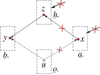
Figure 14: A portrait of $G_{{\stackrel{{\scriptstyle\wedge}}{{{\,\underline{h}\,}}}}.,{\stackrel{{\scriptstyle\wedge}}{{{\,\underline{a}\,}}}}.}$, alluded to in Claim 20.

Note that

$$P(y|{\stackrel{{\scriptstyle\wedge}}{{z}}}) = \sum_{x}{P(y,x|[\;]^{c\wedge})}$$ (101a)

$$= \sum_{x}P(y|z,x)P(x)\;.$$ (101b)

Combining the upsilon values given, Eq.(100) and Eq.(101b), we conclude that Eq.(86), when fully specialized to this example, becomes

$$P(y|{\stackrel{{\scriptstyle\wedge}}{{x}}}) = \sum_{z}\left[\sum_{x^{\prime}}{P(y,x^{\prime}|[\;]^{c\wedge})}\right]P(z|x)$$ (102a)

$$= \sum_{z}\left[\sum_{x^{\prime}}P(y|z,x^{\prime})P(x^{\prime})\right]P(z|x)\;.$$ (102b)

A.3 Example from Ref.[3]-Fig.2

In this example, we want to $P_{{\,\underline{v}\,}.}$ express $P(y|{\stackrel{{\scriptstyle\wedge}}{{x}}})$ for the graph of Fig.15.

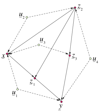
Figure 15: Graph $G$ for Section A.3.

For this example, the following table applies.

$$\begin{array}[]{c||c|c|c|c||c||}&\lx@intercol\hfil\underline{{\cal V}}.={({\,\underline{v}\,}.)_{cc\;0}}\hfil\lx@intercol\vrule\lx@intercol\vrule\lx@intercol&{({\,\underline{v}\,}.)_{cc\;1}}\\ \cline{2-6}\cr&{\,\underline{x}}&{\,\underline{y}}&{\,\underline{z}\,}_{3}&{\,\underline{z}\,}_{2}&{\,\underline{z}\,}_{1}\\ \hline\cr{\,\underline{t}}&\checkmark&&&&\\ \hline\cr{\,\underline{s}\,}.&&\checkmark&&&\\ \hline\cr{\,\underline{d}\,}.&&\checkmark&\checkmark&\checkmark&\checkmark\\ \hline\cr\end{array}\;$$ (103)

One possible topological ordering for the visible nodes ${\,\underline{v}\,}.$ of this graph is

$${\,\underline{y}\,}\leftarrow{\,\underline{z}\,}_{3}\leftarrow{\,\underline{z}\,}_{1}\leftarrow{\,\underline{x}\,}\leftarrow{\,\underline{z}\,}_{2}\;$$ (104)

According to Claim 11,

$$P(v.)={P(y,x,z_{3},z_{2}|[\;]^{c\wedge})}\underbrace{{P(z_{1}|[\;]^{c\wedge})}}_{P(z_{1}|x,z_{2})}\;,$$ (105)

where

$${P(y,x,z_{3},z_{2}|[\;]^{c\wedge})} = \left\langle{P(y|z_{1,3},u_{1,4})P(z_{3}|z_{2},u_{3})P(x|z_{2},u_{1,2,3})P(z_{2}|u_{2,4})}\right\rangle_{u.}$$ (106a)

$$= P(y|z_{3},z_{1},x,z_{2})P(z_{3}|z_{1},x,z_{2})P(x|z_{2})P(z_{2})\;.$$ (106b)

Eq.(86) can be specialized using the data from table Eq.(103) to get the following values for the upsilon terms:

$$\Upsilon_{1}=P(y|{\stackrel{{\scriptstyle\wedge}}{{x}}})\;,$$ (107)

$$\Upsilon_{2}=\sum_{z.}\;,$$ (108)

$$\Upsilon_{3}=P(y,z_{3},z_{2}|{\stackrel{{\scriptstyle\wedge}}{{z}}}_{1},{\stackrel{{\scriptstyle\wedge}}{{x}}})\;,$$ (109)

$$\Upsilon_{4}=P(z_{1}|x,z_{2})\;.$$ (110)

Claim 21

$$P(y,z_{3},z_{2}|{\stackrel{{\scriptstyle\wedge}}{{z}}}_{1},{\stackrel{{\scriptstyle\wedge}}{{x}}})=P(y,z_{3},z_{2}|{\stackrel{{\scriptstyle\wedge}}{{z}}}_{1})\;.$$ (111)

proof:

See Ref.[8] where the 3 Rules of Judea Pearl’s do-calculus are stated. Using the notation there, let ${\,\underline{b}\,}.=({\,\underline{y}\,},{\,\underline{z}\,}_{3},{\,\underline{z}\,}_{2}),{\,\underline{a}\,}.={\,\underline{x}\,},{\,\underline{h}\,}.={\,\underline{z}\,}_{1},{\,\underline{i}\,}.=\emptyset,{\,\underline{o}\,}.={\,\underline{u}\,}.$. Note that ${\,\underline{a}\,}.^{-}={\,\underline{a}\,}.-{\,\underline{an}\,}({\,\underline{i}\,}.,G_{{\stackrel{{\scriptstyle\wedge}}{{{\,\underline{h}\,}}}}.})={\,\underline{a}\,}.$ so $G_{{\stackrel{{\scriptstyle\wedge}}{{{\,\underline{h}\,}}}}.,({\,\underline{a}\,}.^{-})^{\wedge}}=G_{{\stackrel{{\scriptstyle\wedge}}{{{\,\underline{h}\,}}}}.,{\stackrel{{\scriptstyle\wedge}}{{{\,\underline{a}\,}}}}.}$. Fig.16 portrays $G_{{\stackrel{{\scriptstyle\wedge}}{{{\,\underline{h}\,}}}}.,{\stackrel{{\scriptstyle\wedge}}{{{\,\underline{a}\,}}}}.}$. Apply Rule 3 to that figure.
QED

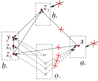
Figure 16: A portrait of $G_{{\stackrel{{\scriptstyle\wedge}}{{{\,\underline{h}\,}}}}.,{\stackrel{{\scriptstyle\wedge}}{{{\,\underline{a}\,}}}}.}$, alluded to in Claim 21.

Note that

$$P(y,z_{3},z_{2}|{\stackrel{{\scriptstyle\wedge}}{{z}}}_{1})=\sum_{x}{P(y,x,z_{3},z_{2}|[\;]^{c\wedge})}\;.$$ (112)

Combining the upsilon values given, Eq.(111) and Eq.(112), we conclude that Eq.(86), when fully specialized to this example, becomes

$$P(y|{\stackrel{{\scriptstyle\wedge}}{{x}}})=\sum_{z.}\left[\sum_{x^{\prime}}{P(y,x^{\prime},z_{3},z_{2}|[\;]^{c\wedge})}\right]P(z_{1}|x,z_{2})\;.$$ (113)

A.4 Example from Ref.[3]-Fig.3

In this example, we want to $P_{{\,\underline{v}\,}.}$ express $P(y|{\stackrel{{\scriptstyle\wedge}}{{x}}})$ for the graph of Fig.17.

Figure 17: Graph $G$ for Section A.4.

For this example, the following table applies.

$$\begin{array}[]{c||c|c||c|c||}&\lx@intercol\hfil\underline{{\cal V}}.={({\,\underline{v}\,}.)_{cc\;0}}\hfil\lx@intercol\vrule\lx@intercol\vrule\lx@intercol&\lx@intercol\hfil{({\,\underline{v}\,}.)_{cc\;1}}\hfil\lx@intercol\vrule\lx@intercol\vrule\lx@intercol\\ \cline{2-5}\cr&{\,\underline{x}}&{\,\underline{z}\,}_{2}&{\,\underline{z}\,}_{1}&{\,\underline{y}}\\ \hline\cr{\,\underline{t}}&\checkmark&&&\\ \hline\cr{\,\underline{s}\,}.&&&&\checkmark\\ \hline\cr{\,\underline{d}\,}.&&\checkmark&\checkmark&\checkmark\\ \hline\cr\end{array}\;$$ (114)

One possible topological ordering for the visible nodes ${\,\underline{v}\,}.$ of this graph is

$${\,\underline{y}\,}\leftarrow{\,\underline{z}\,}_{2}\leftarrow{\,\underline{z}\,}_{1}\leftarrow{\,\underline{x}\,}\;$$ (115)

According to Claim 11,

$$P(v.)={P(z_{2},x|[\;]^{c\wedge})}{P(y,z_{1}|[\;]^{c\wedge})}\;,$$ (116)

where

$${P(z_{2},x|[\;]^{c\wedge})} = \left\langle P(z_{2}|z_{1},u_{1})P(x|u_{1})\right\rangle_{u_{1}}$$ (117a)

$$= P(z_{2}|z_{1},x)P(x)\;,$$ (117b)

and

$${P(y,z_{1}|[\;]^{c\wedge})} = \left\langle P(y|x,z_{2},z_{1},u_{2})P(z_{1}|x,u_{2})\right\rangle_{u_{2}}$$ (118a)

$$= P(y|z_{2},z_{1},x)P(z_{1}|x)\;.$$ (118b)

Eq.(86) can be specialized using the data from table Eq.(114) to get the following values for the upsilon terms:

$$\Upsilon_{1}=P(y|{\stackrel{{\scriptstyle\wedge}}{{x}}})\;,$$ (119)

$$\Upsilon_{2}=\sum_{z_{1},z_{2}}\;,$$ (120)

$$\Upsilon_{3}=P(z_{2}|(z_{1},y)^{\wedge},{\stackrel{{\scriptstyle\wedge}}{{x}}})\;,$$ (121)

$$\Upsilon_{4}={P(y,z_{1}|[\;]^{c\wedge})}\;.$$ (122)

Claim 22

$$P(z_{2}|(z_{1},y)^{\wedge},{\stackrel{{\scriptstyle\wedge}}{{x}}})=P(z_{2}|(z_{1},y)^{\wedge})\;.$$ (123)

proof:

See Ref.[8] where the 3 Rules of Judea Pearl’s do-calculus are stated. Using the notation there, let ${\,\underline{b}\,}.={\,\underline{z}\,}_{2},{\,\underline{a}\,}.={\,\underline{x}\,},{\,\underline{h}\,}.=({\,\underline{z}\,}_{1},{\,\underline{y}\,}),{\,\underline{i}\,}.=\emptyset,{\,\underline{o}\,}.={\,\underline{u}\,}.$. Note that ${\,\underline{a}\,}.^{-}={\,\underline{a}\,}.-{\,\underline{an}\,}({\,\underline{i}\,}.,G_{{\stackrel{{\scriptstyle\wedge}}{{{\,\underline{h}\,}}}}.})={\,\underline{a}\,}.$ so $G_{{\stackrel{{\scriptstyle\wedge}}{{{\,\underline{h}\,}}}}.,({\,\underline{a}\,}.^{-})^{\wedge}}=G_{{\stackrel{{\scriptstyle\wedge}}{{{\,\underline{h}\,}}}}.,{\stackrel{{\scriptstyle\wedge}}{{{\,\underline{a}\,}}}}.}$. Fig.18 portrays $G_{{\stackrel{{\scriptstyle\wedge}}{{{\,\underline{h}\,}}}}.,{\stackrel{{\scriptstyle\wedge}}{{{\,\underline{a}\,}}}}.}$. Apply Rule 3 to that figure.
QED

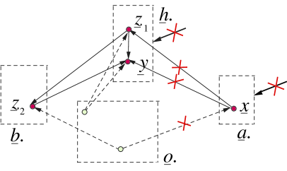
Figure 18: A portrait of $G_{{\stackrel{{\scriptstyle\wedge}}{{{\,\underline{h}\,}}}}.,{\stackrel{{\scriptstyle\wedge}}{{{\,\underline{a}\,}}}}.}$, alluded to in Claim 22.

Note that

$$P(z_{2}|(z_{1},y)^{\wedge})=\sum_{x}{P(z_{2},x|[\;]^{c\wedge})}\;.$$ (124)

Combining the upsilon values given, Eq.(123) and Eq.(124), we conclude that Eq.(86), when fully specialized to this example, becomes

$$P(y|{\stackrel{{\scriptstyle\wedge}}{{x}}})=\sum_{z_{1},z_{2}}\left[\sum_{x^{\prime}}{P(z_{2},x^{\prime}|[\;]^{c\wedge})}\right]{P(y,z_{1}|[\;]^{c\wedge})}\;.$$ (125)

A.5 Example from Ref.[3]-Fig.6

In this example, we want to $P_{{\,\underline{v}\,}.}$ express $P(y|{\stackrel{{\scriptstyle\wedge}}{{x}}})$ for the graph of Fig.19.

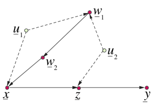
Figure 19: Graph $G$ for Section A.5.

For this example, the following table applies.

$$\begin{array}[]{c||c|c|c||c||c||}&\lx@intercol\hfil\underline{{\cal V}}.={({\,\underline{v}\,}.)_{cc\;0}}\hfil\lx@intercol\vrule\lx@intercol\vrule\lx@intercol&{({\,\underline{v}\,}.)_{cc\;1}}&{({\,\underline{v}\,}.)_{cc\;2}}\\ \cline{2-6}\cr&{\,\underline{x}}&{\,\underline{z}}&{\,\underline{w}\,}_{1}&{\,\underline{w}\,}_{2}&{\,\underline{y}}\\ \hline\cr{\,\underline{t}}&\checkmark&&&&\\ \hline\cr{\,\underline{s}\,}.&&&&&\checkmark\\ \hline\cr{\,\underline{d}\,}.&&\checkmark&&&\checkmark\\ \hline\cr\end{array}\;$$ (126)

One possible topological ordering for the visible nodes ${\,\underline{v}\,}.$ of this graph is

$${\,\underline{y}\,}\leftarrow{\,\underline{z}\,}\leftarrow{\,\underline{x}\,}\leftarrow{\,\underline{w}\,}_{2}\leftarrow{\,\underline{w}\,}_{1}\;$$ (127)

According to Claim 11,

$$P(v.)={P(z,x,w_{1}|[\;]^{c\wedge})}\underbrace{{P(w_{2}|[\;]^{c\wedge})}}_{=P(w_{2}|w_{1})}\underbrace{{P(y|[\;]^{c\wedge})}}_{=P(y|z,x,w_{1,2})=P(y|z)}\;,$$ (128)

where

$${P(z,x,w_{1}|[\;]^{c\wedge})} = \left\langle P(z|x,u_{2})P(x|w_{2},u_{1})P(w_{1}|u_{1},u_{2})\right\rangle_{u_{1},u_{2}}$$ (129a)

$$= P(z|x,w_{2},w_{1})P(x|w_{2},w_{1})P(w_{1})\;.$$ (129b)

Eq.(86) can be specialized using the data from table Eq.(126) to get the following values for the upsilon terms:

$$\Upsilon_{1}=P(y|{\stackrel{{\scriptstyle\wedge}}{{x}}})\;,$$ (130)

$$\Upsilon_{2}=\sum_{z}\;,$$ (131)

$$\Upsilon_{3}=P(z|(w_{2},y)^{\wedge},{\stackrel{{\scriptstyle\wedge}}{{x}}})\;,$$ (132)

$$\Upsilon_{4}=P(y|z)\;.$$ (133)

Claim 23

$$P(z|(w_{2},y)^{\wedge},{\stackrel{{\scriptstyle\wedge}}{{x}}})=P(z|(w_{2},y)^{\wedge},x)\;.$$ (134)

proof:

See Ref.[8] where the 3 Rules of Judea Pearl’s do-calculus are stated. Using the notation there, let ${\,\underline{b}\,}.={\,\underline{z}\,},{\,\underline{a}\,}.={\,\underline{x}\,},{\,\underline{h}\,}.=({\,\underline{w}\,}_{2},{\,\underline{y}\,}),{\,\underline{i}\,}.=\emptyset,{\,\underline{o}\,}.=({\,\underline{w}\,}_{1},{\,\underline{u}\,}_{1},{\,\underline{u}\,}_{2})$. Fig.20 portrays $G_{{\stackrel{{\scriptstyle\wedge}}{{{\,\underline{h}\,}}}}.,{\stackrel{{\scriptstyle\vee}}{{{\,\underline{a}\,}}}}.}$. Apply Rule 2 to that figure.
QED

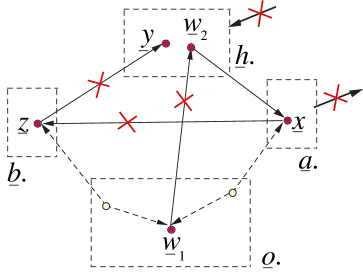
Figure 20: A portrait of $G_{{\stackrel{{\scriptstyle\wedge}}{{{\,\underline{h}\,}}}}.,{\stackrel{{\scriptstyle\vee}}{{{\,\underline{a}\,}}}}.}$, alluded to in Claim 23.

Note that

$$P(z|(w_{2},y)^{\wedge},x)=\frac{\sum_{w_{1}}{P(z,x,w_{1}|[\;]^{c\wedge})}}{\sum_{z}num}\;.$$ (135)

Combining the upsilon values given, Eq.(134) and Eq.(135), we conclude that Eq.(86), when fully specialized to this example, becomes

$$P(y|{\stackrel{{\scriptstyle\wedge}}{{x}}})=\sum_{z}\left[\frac{\sum_{w_{1}}{P(z,x,w_{1}|[\;]^{c\wedge})}}{\sum_{z}num}\right]P(y|z)\;.$$ (136)

Note that the right hand side of the last equation appears to depend on $w_{2}$ but doesn’t.

A.6 3 shark teeth graph with middle tooth missing

In this example, we want to $P_{{\,\underline{v}\,}.}$ express $P(y_{3,1}|{\stackrel{{\scriptstyle\wedge}}{{x}}})$ for the graph of Fig.21. We refer to the set ${\,\underline{y}\,}.$ as teeth and to ${\,\underline{y}\,}_{2}$ as a missing tooth in this example.

Figure 21: Graph $G$ for Section A.6.

For this example, the following table applies.

$$\begin{array}[]{c||c|c|c|c||}&\lx@intercol\hfil\underline{{\cal V}}.={({\,\underline{v}\,}.)_{cc\;0}}\hfil\lx@intercol\vrule\lx@intercol\vrule\lx@intercol\\ \cline{2-5}\cr&{\,\underline{x}}&{\,\underline{y}\,}_{1}&{\,\underline{y}\,}_{2}&{\,\underline{y}\,}_{3}\\ \hline\cr{\,\underline{t}}&\checkmark&&&\\ \hline\cr{\,\underline{s}\,}.&&\checkmark&&\checkmark\\ \hline\cr{\,\underline{d}\,}.&&\checkmark&&\checkmark\\ \hline\cr\end{array}\;$$ (137)

One possible topological ordering for the visible nodes ${\,\underline{v}\,}.$ of this graph is

$${\,\underline{y}\,}_{3}\leftarrow{\,\underline{y}\,}_{2}\leftarrow{\,\underline{y}\,}_{1}\leftarrow{\,\underline{x}\,}\;$$ (138)

According to Claim 11,

$$P(v.)={P(y.,x|[\;]^{c\wedge})}\;,$$ (139)

where

$${P(y.,x|[\;]^{c\wedge})} = \left\langle P(y_{3}|x,u_{3})P(y_{2}|u_{3},u_{2})P(y_{1}|u_{2},u_{1})P(x|u_{1})\right\rangle_{u.}$$ (140a)

$$= P(y_{3}|y_{2},y_{1})P(y_{2}|y_{1},x)P(y_{1}|x)P(x)\;.$$ (140b)

Eq.(86) can be specialized using the data from table Eq.(137) to get the following values for the upsilon terms:

$$\Upsilon_{1}=P(y_{3,1}|{\stackrel{{\scriptstyle\wedge}}{{x}}})\;,$$ (141)

$$\Upsilon_{2}=1\;,$$ (142)

$$\Upsilon_{3}=P(y_{3,1}|{\stackrel{{\scriptstyle\wedge}}{{x}}})\;,$$ (143)

$$\Upsilon_{4}=1\;.$$ (144)

Claim 24

Rule 2 (resp., Rule 3) fails to prove that $P(y_{3,1}|{\stackrel{{\scriptstyle\wedge}}{{x}}})$ equals $P(y_{3,1}|x)$ (resp., $P(y_{3,1})$).

proof:

See Ref.[8] where the 3 Rules of Judea Pearl’s do-calculus are stated. Using the notation there, let ${\,\underline{b}\,}.={\,\underline{y}\,}_{3,1},{\,\underline{a}\,}.={\,\underline{x}\,},{\,\underline{h}\,}.=\emptyset,{\,\underline{i}\,}.=\emptyset,{\,\underline{o}\,}.=({\,\underline{y}\,}_{2},{\,\underline{u}\,}.)$. One can see from Fig.22 that there exists an unblocked path from ${\,\underline{a}\,}.$ to ${\,\underline{b}\,}.$ at fixed $({\,\underline{h}\,}.,{\,\underline{i}\,}.)$ in $G_{{\stackrel{{\scriptstyle\wedge}}{{{\,\underline{h}\,}}}}.,{\stackrel{{\scriptstyle\vee}}{{{\,\underline{a}\,}}}}.}=G_{{\stackrel{{\scriptstyle\vee}}{{{\,\underline{a}\,}}}}.}$ (resp., $G_{{\stackrel{{\scriptstyle\wedge}}{{{\,\underline{h}\,}}}}.,({\,\underline{a}\,}.^{-})^{\wedge}}=G_{{\stackrel{{\scriptstyle\wedge}}{{{\,\underline{a}\,}}}}.}$) so Rule 2 (resp., Rule 3) cannot be used.
QED

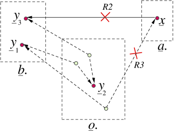
Figure 22: A portrait of $G_{{\stackrel{{\scriptstyle\vee}}{{{\,\underline{a}\,}}}}.}$ for Rule 2 and $G_{{\stackrel{{\scriptstyle\wedge}}{{{\,\underline{a}\,}}}}.}$ for Rule 3, alluded to in Claim 24.

At this point, instead of giving up, we prune the graph $G_{{\,\underline{v}\,}.}$ of Fig.21 to $G_{{\,\underline{v}\,}.^{-}}$ where ${\,\underline{v}\,}.^{-}=\overline{{\,\underline{an}\,}}({\,\underline{y}\,}_{3,1}\cup{\,\underline{x}\,},G_{{\,\underline{v}\,}.})$ to obtain the graph of Fig.23.

Figure 23: Graph $G_{{\,\underline{v}\,}.^{-}}$ for Section A.6.

For this new graph, the following table applies.

$$\begin{array}[]{c||c|c||c||}&\lx@intercol\hfil\underline{{\cal V}}.={({\,\underline{v}\,}.)_{cc\;0}}\hfil\lx@intercol\vrule\lx@intercol\vrule\lx@intercol&{({\,\underline{v}\,}.)_{cc\;1}}\\ \cline{2-4}\cr&{\,\underline{x}}&{\,\underline{y}\,}_{1}&{\,\underline{y}\,}_{3}\\ \hline\cr{\,\underline{t}}&\checkmark&&\\ \hline\cr{\,\underline{s}\,}.&&\checkmark&\checkmark\\ \hline\cr{\,\underline{d}\,}.&&\checkmark&\checkmark\\ \hline\cr\end{array}\;$$ (145)

One possible topological ordering for the visible nodes ${\,\underline{v}\,}.$ of this graph is

$${\,\underline{y}\,}_{3}\leftarrow{\,\underline{y}\,}_{1}\leftarrow{\,\underline{x}\,}\;$$ (146)

According to Claim 11,

$$P(v.)={P(y_{1},x|[\;]^{c\wedge})}\underbrace{{P(y_{3}|[\;]^{c\wedge})}}_{=P(y_{3}|y_{1},x)=P(y_{3}|x)}\;,$$ (147)

where

$${P(y_{1},x|[\;]^{c\wedge})} = \left\langle P(y_{1}|u_{2},u_{1})P(x|u_{1})\right\rangle_{u.}$$ (148a)

$$= P(y_{1}|x)P(x)\;$$ (148b)

Eq.(86) can be specialized using the data from table Eq.(145) to get the following values for the upsilon terms:

$$\Upsilon_{1}=P(y_{3,1}|{\stackrel{{\scriptstyle\wedge}}{{x}}})\;,$$ (149)

$$\Upsilon_{2}=1\;,$$ (150)

$$\Upsilon_{3}=P(y_{1}|{\stackrel{{\scriptstyle\wedge}}{{y_{3}}}},{\stackrel{{\scriptstyle\wedge}}{{x}}})\;,$$ (151)

$$\Upsilon_{4}=P(y_{3}|x)\;.$$ (152)

Claim 25

$$P(y_{1}|{\stackrel{{\scriptstyle\wedge}}{{y_{3}}}},{\stackrel{{\scriptstyle\wedge}}{{x}}})=P(y_{1}|{\stackrel{{\scriptstyle\wedge}}{{y_{3}}}})\;.$$ (153)

proof:

See Ref.[8] where the 3 Rules of Judea Pearl’s do-calculus are stated. Using the notation there, let ${\,\underline{b}\,}.={\,\underline{y}\,}_{1},{\,\underline{a}\,}.={\,\underline{x}\,},{\,\underline{h}\,}.={\,\underline{y}\,}_{3},{\,\underline{i}\,}.=\emptyset,{\,\underline{o}\,}.={\,\underline{u}\,}.$. Note that ${\,\underline{a}\,}.^{-}={\,\underline{a}\,}.-{\,\underline{an}\,}({\,\underline{i}\,}.,G_{{\stackrel{{\scriptstyle\wedge}}{{{\,\underline{h}\,}}}}.})={\,\underline{a}\,}.$ so $G_{{\stackrel{{\scriptstyle\wedge}}{{{\,\underline{h}\,}}}}.,({\,\underline{a}\,}.^{-})^{\wedge}}=G_{{\stackrel{{\scriptstyle\wedge}}{{{\,\underline{h}\,}}}}.,{\stackrel{{\scriptstyle\wedge}}{{{\,\underline{a}\,}}}}.}$. Fig.18 portrays $G_{{\stackrel{{\scriptstyle\wedge}}{{{\,\underline{h}\,}}}}.,{\stackrel{{\scriptstyle\wedge}}{{{\,\underline{a}\,}}}}.}$. Apply Rule 3 to that figure.
QED

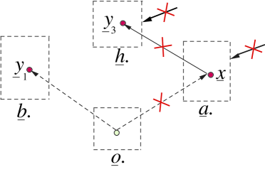
Figure 24: A portrait of $G_{{\stackrel{{\scriptstyle\wedge}}{{{\,\underline{h}\,}}}}.,{\stackrel{{\scriptstyle\wedge}}{{{\,\underline{a}\,}}}}.}$, alluded to in Claim 25.

Note that

$$P(y_{1}|{\stackrel{{\scriptstyle\wedge}}{{y_{3}}}}) = \sum_{x}{P(y_{1},x|[\;]^{c\wedge})}$$ (154a)

$$= P(y_{1})\;.$$ (154b)

Combining the upsilon values given, Eq.(153) and Eq.(154b), we conclude that Eq.(86), when fully specialized to this example, becomes

$$P(y_{3,1}|{\stackrel{{\scriptstyle\wedge}}{{x}}})=P(y_{1})P(y_{3}|x)\;.$$ (155)

Appendix B Appendix- Examples of
Non-identifiable probabilities

In this appendix, we present several examples of non-identifiable uprooted probabilities $P(s.|{\stackrel{{\scriptstyle\wedge}}{{t}}})$. For each example, we will give two specific models which have the same probability of visible nodes $P(v.)$ but which yield different $P(s.|{\stackrel{{\scriptstyle\wedge}}{{t}}})$, thus proving that $P(s.|{\stackrel{{\scriptstyle\wedge}}{{t}}})$ is not $P_{{\,\underline{v}\,}.}$ expressible, and, thus, not identifiable.

One of our examples, the one in Section B.3, is claimed erroneously by Ref.[3] to be an example of an identifiable probability. In Section B.3, we prove that the probability being sought in that case is really not identifiable but the algorithm of Ref.[3] somehow fails to detect this fact.

B.1 One shark tooth graph

In this example, we show that $P(y|{\stackrel{{\scriptstyle\wedge}}{{x}}})$ is not identifiable for the graph of Fig.25.

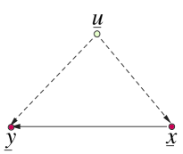
Figure 25: Graph $G$ for Section B.1.

For this example, the following table applies.

$$\begin{array}[]{c||c|c||}&\lx@intercol\hfil\underline{{\cal V}}.={({\,\underline{v}\,}.)_{cc\;0}}\hfil\lx@intercol\vrule\lx@intercol\vrule\lx@intercol\\ \cline{2-3}\cr&{\,\underline{x}}&{\,\underline{y}}\\ \hline\cr{\,\underline{t}}&\checkmark&\\ \hline\cr{\,\underline{s}\,}.&&\checkmark\\ \hline\cr{\,\underline{d}\,}.&&\checkmark\\ \hline\cr\end{array}\;$$ (156)

One possible topological ordering for the visible nodes ${\,\underline{v}\,}.$ of this graph is

$${\,\underline{y}\,}\leftarrow{\,\underline{x}\,}\;$$ (157)

According to Claim 11,

$$P(v.)={P(x,y|[\;]^{c\wedge})}\;,$$ (158)

where

$${P(x,y|[\;]^{c\wedge})} = \left\langle P(y|x,u)P(x|u)\right\rangle_{u}$$ (159a)

$$= P(y|x)P(x)\;.$$ (159b)

Note that

$$P(y|{\stackrel{{\scriptstyle\wedge}}{{x}}})=\left\langle P(y|x,u)\right\rangle_{u}\;,$$ (160)

and

$$P({\cal D}.|{\cal V}.^{c\wedge},{\stackrel{{\scriptstyle\wedge}}{{t}}})=P(y|{\stackrel{{\scriptstyle\wedge}}{{x}}})\;.$$ (161)

Claim 26

Rule 2 (resp., Rule 3) fails to prove that $P(y|{\stackrel{{\scriptstyle\wedge}}{{x}}})$ equals $P(y|x)$ (resp., $P(y)$).

proof:

See Ref.[8] where the 3 Rules of Judea Pearl’s do-calculus are stated. Using the notation there, let ${\,\underline{b}\,}.={\,\underline{y}\,},{\,\underline{a}\,}.={\,\underline{x}\,},{\,\underline{h}\,}.=\emptyset,{\,\underline{i}\,}.=\emptyset,{\,\underline{o}\,}.={\,\underline{u}\,}$. One can see from Fig.26 that there exists an unblocked path from ${\,\underline{a}\,}.$ to ${\,\underline{b}\,}.$ at fixed $({\,\underline{h}\,}.,{\,\underline{i}\,}.)$ in $G_{{\stackrel{{\scriptstyle\wedge}}{{{\,\underline{h}\,}}}}.,{\stackrel{{\scriptstyle\vee}}{{{\,\underline{a}\,}}}}.}=G_{{\stackrel{{\scriptstyle\vee}}{{{\,\underline{a}\,}}}}.}$ (resp., $G_{{\stackrel{{\scriptstyle\wedge}}{{{\,\underline{h}\,}}}}.,({\,\underline{a}\,}.^{-})^{\wedge}}=G_{{\stackrel{{\scriptstyle\wedge}}{{{\,\underline{a}\,}}}}.}$) so Rule 2 (resp., Rule 3) cannot be used.
QED

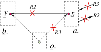
Figure 26: A portrait of $G_{{\stackrel{{\scriptstyle\vee}}{{{\,\underline{a}\,}}}}.}$ for Rule 2 and $G_{{\stackrel{{\scriptstyle\wedge}}{{{\,\underline{a}\,}}}}.}$ for Rule 3, alluded to in Claim 26.

Claim 27

$P(y|{\stackrel{{\scriptstyle\wedge}}{{x}}})$ for the graph of Fig.25 is not identifiable

proof:

Consider a model for the graph of Fig.25 with $y,x,u\in Bool$ and

$$\left\{\begin{array}[]{l}P(y|x,u)=\delta_{y}^{x\wedge u}=\delta_{y}^{xu},\\ P(x|u)=\delta_{x}^{u},\\ P(u)=\frac{1}{2}\end{array}\right.\;.$$ (162)

Note that for this model

$$P(v.)=P(x,y)=\frac{1}{2}\sum_{u}\delta_{y}^{xu}\delta_{x}^{u}=\frac{\delta_{y}^{x}}{2}\;,$$ (163)

and

$$P(y|{\stackrel{{\scriptstyle\wedge}}{{x}}})=\frac{1}{2}\sum_{u}\delta_{y}^{xu}=\frac{\delta_{y}^{0}+\delta_{y}^{x}}{2}\;.$$ (164)

One can define a second model $P^{\prime}$ with

$$\left\{\begin{array}[]{l}P^{\prime}(y|x,u)=P(\overline{y}|\overline{x},u)\\ P^{\prime}(x|u)=P(\overline{x}|u)\\ P^{\prime}(u)=P(u)\end{array}\right.\;.$$ (165)

Note that $P^{\prime}(v.)=\frac{\delta_{y}^{x}}{2}=P(v.)$ but $P^{\prime}(y|{\stackrel{{\scriptstyle\wedge}}{{x}}})=\frac{\delta_{y}^{1}+\delta_{y}^{x}}{2}\neq P(y|{\stackrel{{\scriptstyle\wedge}}{{x}}})$. Hence, there exist two models for the graph of Fig.25 that have the same $P(v.)$ but different $P(y|{\stackrel{{\scriptstyle\wedge}}{{x}}})$. Thus, $P(y|{\stackrel{{\scriptstyle\wedge}}{{x}}})$ is not $P_{{\,\underline{v}\,}.}$ expressible.
QED

Claim 28

There exists a model for the graph of Fig.25 for which $H({\,\underline{y}\,}:{\stackrel{{\scriptstyle\wedge}}{{{\,\underline{x}\,}}}})<0$.

proof:

Consider a model for the graph of Fig.25 with the same node transition probabilities as those given by Eq.(162), except for the following change

$$P(y|x,u)=\delta_{y}^{x\oplus u}\;.$$ (166)

Note that for this model

$$P(v.)=P(x,y)=\frac{1}{2}\sum_{u}\delta_{y}^{x\oplus u}\delta_{x}^{u}=\frac{\delta_{y}^{0}}{2}\;,$$ (167)

and

$$P(y|{\stackrel{{\scriptstyle\wedge}}{{x}}})=\frac{1}{2}\sum_{u}\delta_{y}^{x\oplus u}=\frac{1}{2}\;.$$ (168)

Therefore,

$$H({\,\underline{y}\,}:{\stackrel{{\scriptstyle\wedge}}{{{\,\underline{x}\,}}}})=\sum_{x,y}P(x,y)\ln\frac{P(y|{\stackrel{{\scriptstyle\wedge}}{{x}}})}{P(y)}=\sum_{x,y}\frac{\delta_{y}^{0}}{2}\ln\frac{\frac{1}{2}}{\delta_{y}^{0}}=-\ln 2<0\;.$$ (169)

QED

B.2 3 shark teeth graph (see Appendix A of Ref.[3])

In this example, we show that $P(y.|{\stackrel{{\scriptstyle\wedge}}{{x}}})$ is not identifiable for the graph of Fig.27. This section generalizes the results of the previous section from a graph with “one tooth” to a graph with “3 teeth”. It will become clear as we proceed that the results of this section generalize easily to a graph with an arbitrary number $N\geq 1$ of teeth.

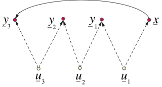
Figure 27: Graph $G$ for Section B.2.

For this example, the following table applies.

$$\begin{array}[]{c||c|c||c||c||}&\lx@intercol\hfil\underline{{\cal V}}.={({\,\underline{v}\,}.)_{cc\;0}}\hfil\lx@intercol\vrule\lx@intercol\vrule\lx@intercol\\ \cline{2-5}\cr&{\,\underline{x}}&{\,\underline{y}\,}_{3}&{\,\underline{y}\,}_{2}&{\,\underline{y}\,}_{1}\\ \hline\cr{\,\underline{t}}&\checkmark&&&\\ \hline\cr{\,\underline{s}\,}.&&\checkmark&\checkmark&\checkmark\\ \hline\cr{\,\underline{d}\,}.&&\checkmark&\checkmark&\checkmark\\ \hline\cr\end{array}\;$$ (170)

One possible topological ordering for the visible nodes ${\,\underline{v}\,}.$ of this graph is

$${\,\underline{y}\,}_{3}\leftarrow{\,\underline{y}\,}_{2}\leftarrow{\,\underline{y}\,}_{1}\leftarrow{\,\underline{x}\,}\;$$ (171)

According to Claim 11,

$$P(v.)={P(y.,x|[\;]^{c\wedge})}\;,$$ (172)

where

$${P(y.,x|[\;]^{c\wedge})} = \left\langle P(y_{3}|x,u_{3})P(y_{2}|u_{3},u_{2})P(y_{1}|u_{2},u_{1})P(x|u_{1})\right\rangle_{u.}$$ (173a)

$$= P(y.|x)P(x)\;.$$ (173b)

Note that

$$P(y.|{\stackrel{{\scriptstyle\wedge}}{{x}}})=\left\langle P(y_{3}|x,u_{3})P(y_{2}|u_{3},u_{2})P(y_{1}|u_{2},u_{1})\right\rangle_{u.}\;,$$ (174)

and

$$P({\cal D}.|{\cal V}.^{c\wedge},{\stackrel{{\scriptstyle\wedge}}{{t}}})=P(y.|{\stackrel{{\scriptstyle\wedge}}{{x}}})\;.$$ (175)

Claim 29

Rule 2 (resp., Rule 3) fails to prove that $P(y.|{\stackrel{{\scriptstyle\wedge}}{{x}}})$ equals $P(y.|x)$ (resp., $P(y.)$).

proof:

See Ref.[8] where the 3 Rules of Judea Pearl’s do-calculus are stated. Using the notation there, let ${\,\underline{b}\,}.={\,\underline{y}\,}.,{\,\underline{a}\,}.={\,\underline{x}\,},{\,\underline{h}\,}.=\emptyset,{\,\underline{i}\,}.=\emptyset,{\,\underline{o}\,}.={\,\underline{u}\,}.$. One can see from Fig.28 that there exists an unblocked path from ${\,\underline{a}\,}.$ to ${\,\underline{b}\,}.$ at fixed $({\,\underline{h}\,}.,{\,\underline{i}\,}.)$ in $G_{{\stackrel{{\scriptstyle\wedge}}{{{\,\underline{h}\,}}}}.,{\stackrel{{\scriptstyle\vee}}{{{\,\underline{a}\,}}}}.}=G_{{\stackrel{{\scriptstyle\vee}}{{{\,\underline{a}\,}}}}.}$ (resp., $G_{{\stackrel{{\scriptstyle\wedge}}{{{\,\underline{h}\,}}}}.,({\,\underline{a}\,}.^{-})^{\wedge}}=G_{{\stackrel{{\scriptstyle\wedge}}{{{\,\underline{a}\,}}}}.}$) so Rule 2 (resp., Rule 3) cannot be used.
QED

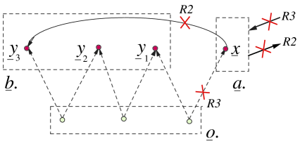
Figure 28: A portrait of $G_{{\stackrel{{\scriptstyle\vee}}{{{\,\underline{a}\,}}}}.}$ for Rule 2 and $G_{{\stackrel{{\scriptstyle\wedge}}{{{\,\underline{a}\,}}}}.}$ for Rule 3, alluded to in Claim 29.

Claim 30

$P(y.|{\stackrel{{\scriptstyle\wedge}}{{x}}})$ for the graph of Fig.27 is not identifiable

proof:

For the graph of Fig.27, we have

$$P(v.)=P(y.,x)=\left\langle P(y_{3}|x,u_{3})P(y_{2}|u_{3},u_{2})P(y_{1}|u_{2},u_{1})P(x|u_{1})\right\rangle_{u.}\;,$$ (176)

and

$$P(y.|{\stackrel{{\scriptstyle\wedge}}{{x}}})=\left\langle P(y_{3}|x,u_{3})P(y_{2}|u_{3},u_{2})P(y_{1}|u_{2},u_{1})\right\rangle_{u.}\;.$$ (177)

Consider $u_{j},x,y_{j}\in Bool$. Let

$$P(u_{j})=\frac{1}{2}\;$$ (178)

for $j=1,2,3$ and

$$P(x|u_{1})=\delta_{x}^{u_{1}}\;.$$ (179)

Also let

$$P(y_{3}|x,u_{3})=\left[M_{3}(y_{3})\right]_{x,u_{3}}\;,$$ (180)

where

$$M_{3}(y_{3})=\Omega\left[\begin{array}[]{cc}(-1)^{y_{3}}&0\\ (-1)^{y_{3}}g_{0}&1\end{array}\right]\Omega^{T}\;.$$ (181)

We will assume that $g_{0}$ is a real number that is much smaller than 1 in absolute value. Note that $\sum_{y_{3}}M_{3}(y_{3})=2{\cal A}=\left[\begin{array}[]{cc}1&1\\ 1&1\end{array}\right]$ as expected since $P(y_{3}|x,u_{3})$ is a probability distribution.

Also let

$$P(y_{2}|u_{3},u_{2})=\left[M_{2}(y_{2})\right]_{u_{3},u_{2}}\;,$$ (182)

where

$$M_{2}(y_{2})=\Omega\left[\begin{array}[]{cc}-(1)^{y_{2}}&0\\ 0&1\end{array}\right]\Omega^{T}\;.$$ (183)

Note that $\sum_{y_{2}}M_{2}(y_{2})=2{\cal A}$ as expected since $P(y_{2}|u_{3},u_{2})$ is a probability distribution.

Also let

$$P(y_{1}|u_{2},u_{1})=\left[M_{1}(y_{1})\right]_{u_{2},u_{1}}\;,$$ (184)

where

$$M_{1}(y_{1})=\Omega\left[\begin{array}[]{cc}(-1)^{y_{1}}&(-1)^{y_{1}}(-g_{0})\\ 0&1\end{array}\right]\Omega^{T}\;.$$ (185)

Note that $\sum_{y_{1}}M_{1}(y_{1})=2{\cal A}$ as expected since $P(y_{1}|u_{2},u_{1})$ is a probability distribution.

When dealing with $N>3$ teeth ${\,\underline{y}\,}_{N},{\,\underline{y}\,}_{N-1},\ldots,{\,\underline{y}\,}_{1}$, one can use

• $M(y_{N})=\Omega(\mbox{ lower triangular matrix })\Omega^{T}$, as we did for $M(y_{3})$ in Eq.(181).

• For $j\in\{N-1,N-2,\ldots,2\}$, $M(y_{j})=\Omega(\mbox{ diagonal matrix })\Omega^{T}$, as we did for $M(y_{2})$ in Eq.(183).

• $M(y_{1})=\Omega(\mbox{ upper triangular matrix })\Omega^{T}$, as we did for $M(y_{1})$ in Eq.(185).

If we define

$$M(y.)=M_{3}(y_{3})M_{2}(y_{2})M_{1}(y_{1})\;,$$ (186)

then

$$P(y.,x)=\frac{1}{2^{3}}[M(y.)]_{x,x}\;,$$ (187)

and

$$P(y.|{\stackrel{{\scriptstyle\wedge}}{{x}}})=\frac{1}{2^{3}}\sum_{u_{1}}[M(y.)]_{x,u_{1}}=\frac{1}{2^{3}}\left([M(y.)]_{x,x}+[M(y.)]_{x,\overline{x}}\right)\;.$$ (188)

(As usual, $\overline{x}=1-x$). Let

$$\sigma=(-1)^{y_{1}+y_{2}+y_{3}}\;.$$ (189)

Then

$$M(y.) = \Omega\left[\begin{array}[]{cc}\sigma&\sigma(-g_{0})\\ \sigma g_{0}&1-\sigma g_{0}^{2}\end{array}\right]\Omega^{T}$$ (190c)

$$= (1-\sigma g_{0}^{2}){\cal A}+\sigma\left[\begin{array}[]{cc}0&-g_{0}\\ g_{0}&0\end{array}\right]+\frac{\sigma}{2}\left[\begin{array}[]{cc}1&-1\\ -1&1\end{array}\right]\;,$$ (190h)

so

$$P(y.,x)=\frac{1}{2^{4}}[1+\sigma(1-g_{0}^{2})]\;,$$ (191)

and

$$P(y.|{\stackrel{{\scriptstyle\wedge}}{{x}}})=\frac{1}{2^{3}}\left[1-\sigma g_{0}((-1)^{x}+g_{0})\right]\;.$$ (192)

Let $0<|g_{0}|<<1$. To first order in $g_{0}$, when we change $g_{0}$, $P(y.,x)$ remains fixed but $P(y.|{\stackrel{{\scriptstyle\wedge}}{{x}}})$ changes. Thus, $P(y|{\stackrel{{\scriptstyle\wedge}}{{x}}})$ is not $P_{{\,\underline{v}\,}.}$ expressible.
QED

Claim 31

There exists a model for the graph of Fig.27 for which $H({\,\underline{y}\,}.:{\stackrel{{\scriptstyle\wedge}}{{{\,\underline{x}\,}}}})<0$.

proof:

Consider a model for the graph of Fig.27 with $u_{j},y_{j},x\in Bool$ and

$$\left\{\begin{array}[]{l}P(u_{j})=\frac{1}{2}\mbox{ for }j=1,2,3\\ P(x|u_{1})=\delta_{x}^{u_{1}}\\ P(y_{3}|x,u_{3})=\delta_{y_{3}}^{x\oplus u_{3}}\\ P(y_{j}|u_{j+1},u_{j})=\delta_{y_{j}}^{u_{j+1}\oplus u_{j}}\mbox{ for }j=2,1\end{array}\right.\;.$$ (193)

Note that for this model

$$P(v.)=P(y.,x) = \frac{1}{2^{3}}\sum_{u.}\delta_{y_{3}}^{x\oplus u_{3}}\delta_{y_{2}}^{u_{3}\oplus u_{2}}\delta_{y_{1}}^{u_{2}\oplus u_{1}}\delta_{x}^{u_{1}}$$ (194a)

$$= \frac{\delta_{y_{3}\oplus y_{2}\oplus y_{1}}^{0}}{2^{3}}\;,$$ (194b)

and

$$P(y.|{\stackrel{{\scriptstyle\wedge}}{{x}}}) = \frac{1}{2^{3}}\sum_{u.}\delta_{y_{3}}^{x\oplus u_{3}}\delta_{y_{2}}^{u_{3}\oplus u_{2}}\delta_{y_{1}}^{u_{2}\oplus u_{1}}$$ (195a)

$$= \frac{1}{2^{3}}\;.$$ (195b)

Therefore,

$$H({\,\underline{y}\,}.:{\stackrel{{\scriptstyle\wedge}}{{{\,\underline{x}\,}}}}) = \sum_{y.,x}P(y.,x)\ln\frac{P(y.|{\stackrel{{\scriptstyle\wedge}}{{x}}})}{P(y.)}$$ (196a)

$$= \sum_{y.,x}\frac{\delta_{y_{3}\oplus y_{2}\oplus y_{1}}^{0}}{2^{3}}\ln\frac{\frac{1}{2^{3}}}{\frac{1}{2^{2}}\delta_{y_{3}\oplus y_{2}\oplus y_{1}}^{0}}$$ (196b)

$$= -\ln(2)\sum_{y.}\frac{\delta_{y_{3}\oplus y_{2}\oplus y_{1}}^{0}}{2^{2}}=-\ln 2<0\;.$$ (196c)

QED

The results of this section concerning the non-identifiability of $P(y.|{\stackrel{{\scriptstyle\wedge}}{{x}}})$ for the N shark teeth graph of Fig.27 apply as well to what I call “modified N shark teeth” graphs, an example of which is given in Fig.29. For the graph $G_{mod}$ of Fig.29, $P(y.|{\stackrel{{\scriptstyle\wedge}}{{x_{3}}}})$ is not identifiable. To show this one can use the same models that we used in the unmodified case, but with $P(x_{3}|x_{2})=\delta_{x_{3}}^{x_{2}}$, and $P(x_{2}|x_{1})=\delta_{x_{2}}^{x_{1}}$.

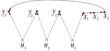
Figure 29: Modified 3 shark teeth graph $G_{mod}$ mentioned in Section B.2.

B.3 Example from Ref.[3]-Fig.9

In this example, we show that $P(y|{\stackrel{{\scriptstyle\wedge}}{{x}}})$ is not identifiable for the graph of Fig.30.

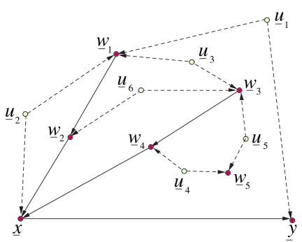
Figure 30: Graph $G$ for Section B.3.

For this example, the following table applies.

$$\begin{array}[]{c||c|c|c||}&\lx@intercol\hfil\underline{{\cal V}}.={({\,\underline{v}\,}.)_{cc\;0}}\hfil\lx@intercol\vrule\lx@intercol\vrule\lx@intercol\\ \cline{2-4}\cr&{\,\underline{x}}&{\,\underline{y}}&{\,\underline{w}\,}.\\ \hline\cr{\,\underline{t}}&\checkmark&&\\ \hline\cr{\,\underline{s}\,}.&&\checkmark&\\ \hline\cr{\,\underline{d}\,}.&&\checkmark&\\ \hline\cr\end{array}\;$$ (197)

One possible topological ordering for the visible nodes ${\,\underline{v}\,}.$ of this graph is

$${\,\underline{y}\,}\leftarrow{\,\underline{x}\,}\leftarrow{\,\underline{w}\,}_{2}\leftarrow{\,\underline{w}\,}_{4}\leftarrow{\,\underline{w}\,}_{1}\leftarrow{\,\underline{w}\,}_{3}\leftarrow{\,\underline{w}\,}_{5}\;$$ (198)

According to Claim 11,

$$P(v.)={P(y,x,w.|[\;]^{c\wedge})}\;$$ (199)

where

$${P(y,x,w.|[\;]^{c\wedge})} = \left\langle\begin{array}[]{l}P(y|x,u_{1})P(x|w_{2,4},u_{2})P(w_{2}|w_{1},u_{6})P(w_{4}|w_{3},u_{4})\\ P(w_{1}|u_{1,2,3})P(w_{3}|u_{3,5,6})P(w_{5}|u_{4,5})\end{array}\right\rangle_{u.}$$ (200c)

$$= P(y,x|w.)P(w.)\;.$$ (200d)

Note that

$$P({\cal D}.|{\cal V}.^{c\wedge},{\stackrel{{\scriptstyle\wedge}}{{t}}})=P(y|{\stackrel{{\scriptstyle\wedge}}{{x}}})\;.$$ (201)

Claim 32

Rule 2 (resp., Rule 3) fails to prove that $P(y|{\stackrel{{\scriptstyle\wedge}}{{x}}})$ equals $P(y|x)$ (resp., $P(y)$).

proof:

See Ref.[8] where the 3 Rules of Judea Pearl’s do-calculus are stated. Using the notation there, let ${\,\underline{b}\,}.={\,\underline{y}\,},{\,\underline{a}\,}.={\,\underline{x}\,},{\,\underline{h}\,}.=\emptyset,{\,\underline{i}\,}.=\emptyset,{\,\underline{o}\,}.=({\,\underline{u}\,}.,{\,\underline{w}\,}.)$. One can see from Fig.31 that there exists an unblocked path from ${\,\underline{a}\,}.$ to ${\,\underline{b}\,}.$ at fixed $({\,\underline{h}\,}.,{\,\underline{i}\,}.)$ in $G_{{\stackrel{{\scriptstyle\wedge}}{{{\,\underline{h}\,}}}}.,{\stackrel{{\scriptstyle\vee}}{{{\,\underline{a}\,}}}}.}=G_{{\stackrel{{\scriptstyle\vee}}{{{\,\underline{a}\,}}}}.}$ (resp., $G_{{\stackrel{{\scriptstyle\wedge}}{{{\,\underline{h}\,}}}}.,({\,\underline{a}\,}.^{-})^{\wedge}}=G_{{\stackrel{{\scriptstyle\wedge}}{{{\,\underline{a}\,}}}}.}$) so Rule 2 (resp., Rule 3) cannot be used.
QED

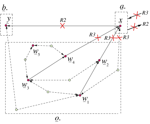
Figure 31: A portrait of $G_{{\stackrel{{\scriptstyle\vee}}{{{\,\underline{a}\,}}}}.}$ for Rule 2 and $G_{{\stackrel{{\scriptstyle\wedge}}{{{\,\underline{a}\,}}}}.}$ for Rule 3, alluded to in Claim 32.

Claim 33

$P(y|{\stackrel{{\scriptstyle\wedge}}{{x}}})$ for the graph of Fig.30 is not identifiable

proof:

Consider a model for the graph of Fig.30 such that

$$\left\{\begin{array}[]{l}P(w_{j}|pa({\,\underline{w}\,}_{j}))=P(w_{j})\mbox{ for }j=3,4,5\\ P(w_{2}|pa({\,\underline{w}\,}_{2}))=\delta_{w_{2}}^{w_{1}}\\ P(w_{1}|u_{1,2,3})=P(w_{1}|u_{1})\\ P(x|pa({\,\underline{x}\,}))=\delta_{x}^{w_{2}}\end{array}\right.\;.$$ (202)

For such a model,

$$P(x,y,w.)=\left\langle P(y|u_{1},x)\delta_{x}^{w_{2}}P(w_{1}|u_{1})\delta_{w_{2}}^{w_{1}}P(w_{3,4,5})\right\rangle_{u_{1}}\;$$ (203)

so

$$P(x,y)=\left\langle P(y|u_{1},x)P({\,\underline{w}\,}_{1}=x|u_{1})\right\rangle_{u_{1}}\;.$$ (204)

This is the same $P(x,y)$ that we obtained in the one shark tooth example that we considered in Section B.1. In that section we learned that $P(y|{\stackrel{{\scriptstyle\wedge}}{{x}}})$ for that graph is not identifiable.
QED

Claim 34

There exists a model for the graph of Fig.30 for which $H({\,\underline{y}\,}:{\stackrel{{\scriptstyle\wedge}}{{{\,\underline{x}\,}}}})<0$.

proof:

In the previous claim, we showed that for the graph of Fig.30, one can define a special type of model for which $P(x,y)$ corresponds to the one shark tooth example of Section B.1. In that section we gave a model for which $H({\,\underline{y}\,}:{\stackrel{{\scriptstyle\wedge}}{{{\,\underline{x}\,}}}})=-\ln(2)$.
QED

References

- [1] Daphne Koller, Nir Friedman, Probabilistic Graphical Models, Principles and Techniques (MIT Press, 2009)
- [2] J. Pearl, “Causal diagrams for empirical research”, R-218-B. (available in pdf format at J. Pearl’s website) Biometrika 82, 669-710 (1995)
- [3] J. Tian, J. Pearl, “On the identification of causal effects”, Technical Report R-290-L
- [4] J. Tian, J. Pearl, “A general identification condition for causal effects”, Eighteenth National Conference on AI, pp.567-573, 2002. (This is just an abridged version of Ref.[3]).
- [5] Y. Huang, M. Valtorta, “Pearl’s calculus of interventions is complete”, Proceedings of the 22 Conference on Uncertainty in Artificial Intelligence, AUAI Press, July 2006
- [6] I Shpitser, J. Pearl, “Identification of conditional interventional distributions”, Proceedings of the 22 Conference on Uncertainty in Artificial Intelligence, AUAI Press, July 2006
- [7] Maxim Raginsky, “Directed Information and Pearl’s Causal Calculus”, arXiv:1110.0718
- [8] Robert R. Tucci, “Introduction to Judea Pearl’s Do-Calculus”, arXiv:1305.5506