A Chandra/HETGS Census of X-ray Variability From Sgr A${}^{*}$ During 2012

Abstract

We present the first systematic analysis of the X-ray variability of Sgr A${}^{*}$ during the Chandra X-ray Observatory’s 2012 Sgr A${}^{*}$ X-ray Visionary Project (XVP). With 38 High Energy Transmission Grating Spectrometer (HETGS) observations spaced an average of 7 days apart, this unprecedented campaign enables detailed study of the X-ray emission from this supermassive black hole at high spatial, spectral and timing resolution. In 3 Ms of observations, we detect 39 X-ray flares from Sgr A${}^{*}$, lasting from a few hundred seconds to approximately 8 ks, and ranging in $2-10$ keV luminosity from $\sim 10^{34}$ erg s${}^{-1}$ to $2\times 10^{35}$ erg s${}^{-1}.$ Despite tentative evidence for a gap in the distribution of flare peak count rates, there is no evidence for X-ray color differences between faint and bright flares. Our preliminary X-ray flare luminosity distribution $dN/dL$ is consistent with a power law with index $-1.9^{+0.3}_{-0.4}$; this is similar to some estimates of Sgr A${}^{*}$’s NIR flux distribution. The observed flares contribute one-third of the total X-ray output of Sgr A${}^{*}$ during the campaign, and as much as 10% of the quiescent X-ray emission could be comprised of weak, undetected flares, which may also contribute high-frequency variability. We argue that flares may be the only source of X-ray emission from the inner accretion flow.

1. INTRODUCTION

Since the launch of the Chandra X-ray Observatory and XMM-Newton in 1999, X-ray observations of Sgr A${}^{*}$, the $4\times 10^{6}M_{\odot}$ black hole at the center of our Galaxy, have revealed a supermassive black hole deep in quiescence, a profound inactivity punctuated roughly once a day by rapid flares (e.g. Baganoff01; Melia01; Baganoff03; Genzel10; Markoff10 and references therein). But rather than clarifying the nature of the X-ray emission, the flares from Sgr A${}^{*}$ have added to the puzzle of its extremely low luminosity.

In weakly accreting black hole systems at all mass scales, there is a well-known three-way correlation between black hole mass, X-ray luminosity, and radio luminosity (the fundamental plane of black hole activity; Merloni03; Falcke04; Kording06; Gultekin09; see also Gallo06; Yuan09). However, as demonstrated by Markoff05b; Kording06; Plotkin12, Sgr A${}^{*}$ only lies on (or near) this fundamental plane during its X-ray flares; in quiescence, the supermassive black hole is a notable outlier. Thus it is evident that studies of the quiescent emission and the flare emission from Sgr A${}^{*}$ probe inherently different physical processes, and that through the flares, we can explore the connections between Sgr A${}^{*}$ and weakly accreting black holes, such as those in low-luminosity AGN (LLAGN, e.g. Ho08; Markoff10; Yuan11 and references therein). The rarity of strong flares in other LLAGN (such as M81: Markoff08; M31: Garcia10, although see Li11; see also Yuan04) places Sgr A${}^{*}$ in a unique position (apparently unable to produce continuous X-ray emission in accordance with the fundamental plane) and highlights the importance of understanding the physics of flares.

One such flare (Nowak12) began on 2012 February 9 around 14:28:19 (UTC). With Chandra looking on, the $2-10$ keV X-ray luminosity rose by a factor of at least $\sim 130$ over the course of an hour, reaching a value of about $5\times 10^{35}$ erg s${}^{-1}$ for a distance of 8 kpc. At its peak, the X-ray emission from this flare (the brightest X-ray flare ever observed from Sgr A${}^{*}$) equaled the normal bolometric luminosity of this supermassive black hole. Within another 30 minutes, it had vanished. But beyond the strong variability on short time scales, what makes this flare and its record-breaking intensity so remarkable is that it topped out at a maximum luminosity of $10^{-9}L_{\rm Edd}$ (still far below the luminosities originally studied on the fundamental plane; see also Porquet03). The majority of X-ray flares, however, are much fainter, with average luminosities around $10\times$ the quiescent level.

A summary of the phenomenology of flares from Sgr A${}^{*}$ is provided by Dodds-Eden09. Studies of the Galactic Center detect approximately four times more flares in the near-infrared (NIR) band than in X-rays (e.g. Genzel03; Eckart06); the evidence suggests that every X-ray flare is accompanied by a more-or-less simultaneous NIR flare, while some NIR flares have no X-ray counterpart (e.g. Hornstein07). In addition, while the spectral indices in these bands are similar, the X-ray flux as seen by Chandra, XMM-Newton, and Swift is not necessarily consistent with the extrapolated NIR spectrum (e.g. Eckart06). In both the infrared (e.g. Hornstein07; Bremer11) and the X-ray (Porquet03; Porquet08; Nowak12; Degenaar12_arxiv), there has been some debate regarding the dependence of the flares’ spectral indices on luminosity. Given the complex relationship between the NIR and X-ray emission, these dependences may be key to understanding flare physics.

Despite the focused attention on both the quiescent X-ray emission and the flares from Sgr A${}^{*}$ during the last decade, neither is completely understood. For reference, the quiescent emission includes all X-ray emission within $1.25\arcsec\approx 6400$ AU $\approx 1.6\times 10^{5}R_{g}$ of Sgr A${}^{*}$, where $R_{g}=GM_{\rm BH}/c^{2}$ is the gravitational radius and $M_{\rm BH}$ is the black hole mass. This includes not only any emission from the hot inner accretion flow, but also from the rest of the accretion flow on scales approaching the Bondi radius (as well as stars, compact objects, and extended diffuse emission integrated along the line of sight, but see Section LABEL:sec:flarepsf and Shcherbakov10). The quiescent X-ray spectrum can be fitted as thermal bremsstrahlung ($kT=2-3.5$ keV), and has shown so little variability over the last 14 years of monitoring that the only plausible physical scenarios for its origin are thermal plasma from large scales or a cluster of coronally active stars (e.g. Falcke00; Quataert02; Baganoff03; Yuan02; Yuan03; Liu04; Xu06; Sazonov12; Nowak12; but see Wang13, in press).

A rich diversity of models has been proposed to explain the flares, both in terms of their energy injection mechanisms, ranging from magnetic reconnection, stochastic acceleration, or shocks in the accretion flow or jet to tidal disruption of asteroids, and in terms of their radiation mechanisms, for which the X-ray photon index $\Gamma\sim 2$ could be due to direct synchrotron, synchrotron self-Compton (SSC), or inverse Compton processes (e.g. Markoff01; Liu02; Liu04; Yuan03; Yuan04; Eckart04; Eckart06; Marrone08; Cadez08; Kostic09; Dodds-Eden09; Yuan09b; Zubovas12; Witzel12; Yusef-Zadeh12; Nowak12 and references therein). The reduced rate of X-ray flares relative to the NIR may be explained if the high-energy emission is dominated by SSC, such that only events for which the column density of synchrotron-emitting electrons is sufficiently large will produce X-ray flares observable above the quiescent emission (e.g. Marrone08 and references therein).

In order to address both the origin of the quiescent emission and the physics of the flares (as well as to continue detailed study of diffuse emission and transients in the Galactic Center; e.g. Baganoff03; Muno04; Park04; Muno07; Muno09; Ponti10; Capelli12), Chandra undertook an unprecedented X-ray Visionary Project (XVP) in 2012 to observe Sgr A${}^{*}$ for 3 Ms at high spectral resolution with the High Energy Transmission Grating Spectrometer (HETGS; C05). The excellent X-ray spectral resolution provides a robust probe of the nature of the accretion flow (Xu06; Young07; Sazonov12), and the high cadence and coverage of observations and the long exposure time are ideal for the first-ever systematic study of X-ray variability and flares from Sgr A${}^{*}$.

This paper is the first systematic study of X-ray flares from Sgr A${}^{*}$ during the 2012 Chandra XVP. Here we focus on quantifying the properties (i.e. intensity and duration) of the flares observed during our 38 Chandra observations and characterizing the relationship between the quiescent emission and the X-ray flares. Although prior Chandra, XMM-Newton, and Swift observations have detected many flares, they used different detectors and have very different spectral responses and levels of pileup (Section 4.1.1); we leave a comprehensive analysis for future work. The paper is organized as follows. In Sections 2 and 3 we describe the Chandra observations and data reduction and our method for identifying flares. In Section 4, we assess the statistical properties of the flares, including their peak brightnesses, fluences, durations, estimated luminosities, and X-ray colors. We also explore the variability caused by undetected flares. In Section LABEL:sec:discuss, we discuss our results in the context of flare models, multiwavelength flux distributions, and the contribution of weak flares to the quiescent X-ray emission.

2. OBSERVATIONS AND DATA REDUCTION

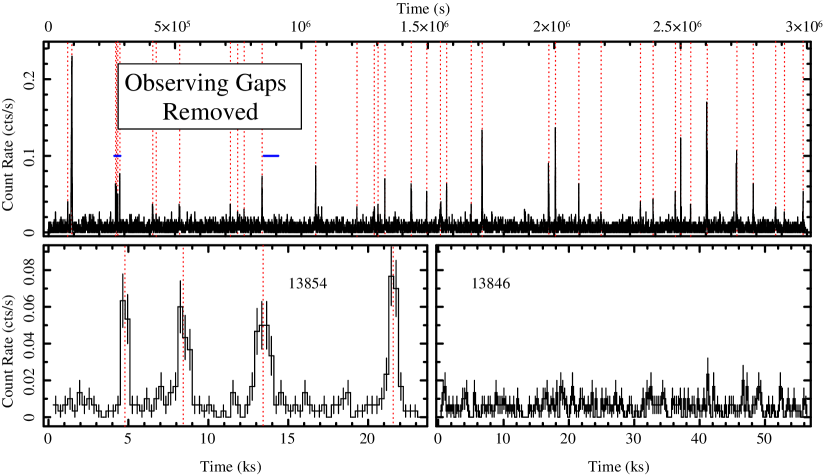
Figure 1.— (Top): Combined zeroth and $1^{\rm st}$ order 2–8 keV Chandra X-ray lightcurve of Sgr A${}^{*}$ in 300 s bins for the entire 2012 XVP campaign with gaps removed; events are extracted from a 2.5 pixel radius circular region around the source for the zeroth order and 5 pixel wide rectangular regions for the $1^{\rm st}$ order lightcurves. A number of flares of varying intensity are apparent, and are indicated by dotted red lines. Short blue horizontal lines indicate sample observations shown in the bottom panel. (Bottom): Sample lightcurves of an observation with (left) and without (right) detected flares. ObsID 13854 (left) shows four moderately bright flares within 20 ks.

During the 2012 XVP campaign, Chandra observed Sgr A${}^{*}$ 38 times at high spectral resolution with the HETGS. The observations, detailed in Table 1, took place between 2012 February 6 and October 29, with exposure times ranging from 14.53 ks to 189.25 ks. For thermal reasons, only five of the chips from the Advanced CCD Imaging Spectrometer-Spectroscopy array (ACIS-S) were used during the campaign (S0 was turned off). We reduce the data with standard tools from the ciao analysis suite, version 4.5. The HETGS consists of two transmission gratings, the High Energy Grating (HEG) and the Medium Energy Grating (MEG), which disperse a fraction of the incoming photons across the detector. With five chips, each detected photon is recorded to a timing accuracy of 3.14 seconds, along with its energy as measured by ACIS and its wavelength and diffraction order as determined by the diffraction equation and the tg_resolve_events tool. To study the X-ray variablility of Sgr A${}^{*}$, we extract 2–8 keV lightcurves of these events in 300-s bins, including only photons in the zeroth order (i.e. the undispersed photons) and the HEG and MEG $\pm 1^{\rm st}$ orders (hereafter $1^{\rm st}$ order photons). All our subsequent timing analysis is done in the Interactive Spectral Interpretation System (ISIS; HD00; Houck02).

As reported in Nowak12, a number of X-ray flares are detected in these observations. It is an impossible task to distinguish the Sgr A${}^{*}$ photons from the underlying diffuse emission. However, the short flare time scales and the absence of associated optically thin radio flares (Section 4; Baganoff01) argue that the flare emission arises from close to the black hole. For our purposes, then, it is sufficient to minimize the background by using small extraction regions as in Nowak12: a $\sim 2.5$ pixel (1.25″) radius circle for the zeroth-order events, 5 pixel wide rectangular regions for the $1^{\rm st}$ order photons, and grating order tolerances of $\pm 0.2.$ Since much of the background emission is found in the $1^{\rm st}$ order (Section 4), a search of the zeroth order alone would also have good sensitivity to flares. But the $1^{\rm st}$ order is essential for pileup calibration (Section 4.1.1), and we prefer to use the same events to detect, characterize, and calibrate our flares.

3. LIGHTCURVES AND FLARE DETECTION

The resulting X-ray lightcurves are shown in Figure 1. For observations spread over nine months and a number of spacecraft roll angles (which affects the diffuse emission in the grating extraction regions), there is remarkably little variation in the quiescent level (Table 1). Highlighting the stability of the baseline emission are the numerous narrow flares, which appear in over half of the 2012 observations (Table 1). Most apparent is the large flare early in the campaign, described in detail in Nowak12, which is the brightest X-ray flare ever observed from Sgr A${}^{*}$ (see also Porquet03). Figure 1 includes several comparably bright flares and numerous moderate and weak flares. One 2-day observation (ObsID 13840) contains no flares, which is consistent with the average rate of $\sim 1$ flare per day (Section LABEL:sec:discuss).

In order to detect and characterize these X-ray flares, we use an algorithm based on direct fits to the X-ray lightcurves shown in Figure 1. There are systematic uncertainties associated with any particular choice of search algorithm; the robustness of our search and an alternative method (the Bayesian Blocks routine; Scargle12_arxiv) are discussed in the Appendix. Here, we fit the 2–8 keV lightcurves with a model consisting of a constant baseline and Gaussian components to represent the flares. Because the count rates are small, we use the Cash statistic (Cash79) and the subplex fit method.

After a first pass to estimate the baseline count rate, we perform an automated search for narrow flares on an observation-by-observation basis. In the algorithm, each time bin is examined: if the count rate is below the (fixed) quiescent level, it is ignored (see Section LABEL:sec:flarevar for a comparison of the data to a Poisson process). Otherwise, we add a “flare” at the center of the bin: a faint narrow Gaussian with an initial 1$\sigma$ width $\sigma_{\rm t}=150$ s. We fit for the flare amplitude and then allow $\sigma_{\rm t}$ to vary as well. We restrict $\sigma_{t}$ to be between 100 s and 1600 s (empirically-determined limits, below which the bin size starts to become large relative to the flare FWHM and above which confusion from nearby flares can interfere with the search process). If the resulting amplitude is larger than the quiescent level at 99% confidence for a single trial, the Gaussian component is identified as a real flare, and we fit for the best amplitude, center, and width.

Because the brightest flare (Nowak12) showed marked asymmetry, we also perform a search for time substructure in the detected flares. Leaving the initial (significant) component free, we add additional “subflares” as above, with flare center times constrained to occur within $\pm 2\sigma_{\rm t}$ of the main component, until additional substructure is no longer significant at the 90% level. The substructure is equally likely to appear before and after the peak. Finally, once all flares and substructure have been identified, we calculate 90% confidence limits for each parameter, including the background level. We define the start (stop) time of a flare to be the minimum (maximum) value of the $2\sigma_{\rm t}$ lower (upper) limits for all its subflares. For each flare, we tabulate the start and stop times, durations, background count rates, rise and decay times, and note whether the flare was truncated by the beginning or end of an observation. We use customized models to fit for the peak count rate and the fluence within the start and stop times of each flare directly (fitting for these parameters and their uncertainties is faster and more reliable than combining all the subflares and propagating their uncertainties).

Table 12012 Chandra XVP Observations of Flares from Sgr A${}^{*}$

	Obs Start	Exp.	Bkg.	Flare	Flare	Fluence	Peak Rate	Duration	# Sub-
ObsID	(MJD)	(ks)	Rate	Start	Stop	(cts)	(cts/s)	(s)	Flares	$F_{2-8}^{\rm abs}$	$L_{2-10}^{\rm unabs}$
13850	55963.026	60.06	$5.9\pm 0.5$	$\cdots$	$\cdots$	$\cdots$	$\cdots$	$\cdots$	$\cdots$	$\cdots$	$\cdots$
14392	55966.262	59.25	$6.2\pm 0.6$	55966.433	55966.464	$33^{+12}_{-11}$	$0.021^{+0.011}_{-0.008}$	2600	1	0.8	1.7
				55966.603	55966.666	$706^{+46}_{-44}$	$0.23\pm 0.03$	5450	4	8.5	19.2
14394	55967.136	18.06	$6.2^{+1.0}_{-0.9}$	$\cdots$	$\cdots$	$\cdots$	$\cdots$	$\cdots$	$\cdots$	$\cdots$	$\cdots$
14393	55968.426	41.55	$7.7\pm 0.7$	$\cdots$	$\cdots$	$\cdots$	$\cdots$	$\cdots$	$\cdots$	$\cdots$	$\cdots$
13856	56001.365	40.06	$5.6\pm 0.6$	$\cdots$	$\cdots$	$\cdots$	$\cdots$	$\cdots$	$\cdots$	$\cdots$	$\cdots$
13857	56003.373	39.56	$6.8\pm 0.7$	$\cdots$	$\cdots$	$\cdots$	$\cdots$	$\cdots$	$\cdots$	$\cdots$	$\cdots$
13854	56006.425	23.06	$5.7\pm 1.0$	56006.486	56006.493	$32^{+11}_{-9}$	$0.06^{+0.03}_{-0.02}$	600	1	3.3	7.4
				56006.524	56006.540	$40^{+12}_{-10}$	$0.05^{+0.02}_{-0.01}$	1350	1	1.8	4.1
				56006.580	56006.599	$49^{+13}_{-12}$	$0.05^{+0.02}_{-0.01}$	1600	1	1.9	4.2
				56006.678	56006.690	$49^{+13}_{-14}$	$0.07^{+0.03}_{-0.02}$	950	1	3.1	7.1
14413	56007.281	14.72	$6.1^{+1.1}_{-1.0}$	$\cdots$	$\cdots$	$\cdots$	$\cdots$	$\cdots$	$\cdots$	$\cdots$	$\cdots$
13855	56008.476	20.06	$6.7^{+1.0}_{-0.9}$	$\cdots$	$\cdots$	$\cdots$	$\cdots$	$\cdots$	$\cdots$	$\cdots$	$\cdots$
14414	56009.742	20.06	$6.3\pm 0.9$	$\cdots$	$\cdots$	$\cdots$	$\cdots$	$\cdots$	$\cdots$	$\cdots$	$\cdots$
13847	56047.678	154.07	$6.0\pm 0.3$	56048.510	56048.548	$59^{+16}_{-14}$	$0.03^{+0.02}_{-0.01}$	3250	3	1.1	2.5
				56048.679	56048.693	$15^{+8}_{-7}$	$0.020^{+0.015}_{-0.010}$	1200	1	0.7	1.7
14427	56053.834	80.06	$6.8\pm 0.5$	56054.107	56054.154	$49^{+15}_{-13}$	$0.03^{+0.02}_{-0.01}$	4050	2	0.7	1.6
13848	56056.502	98.16	$6.2\pm 0.4$	$\cdots$	$\cdots$	$\cdots$	$\cdots$	$\cdots$	$\cdots$	$\cdots$	$\cdots$
13849	56058.138	178.75	$6.7\pm 0.3$	56058.687	56058.705	$24^{+10}_{-11}$	$0.03\pm 0.01$	1600	1	0.9	2.0
				56059.006	56059.044	$33^{+15}_{-11}$	$0.017^{+0.010}_{-0.007}$	3250	1	0.6	1.4
				56059.314	56059.329	$21^{+10}_{-8}$	$0.03^{+0.02}_{-0.01}$	1250	1	1.0	2.3
				56060.127	56060.168	$124^{+21}_{-19}$	$0.06\pm 0.01$	3500	1	2.2	4.9
13846	56063.445	56.21	$6.0^{+0.6}_{-0.5}$	$\cdots$	$\cdots$	$\cdots$	$\cdots$	$\cdots$	$\cdots$	$\cdots$	$\cdots$
14438	56065.187	25.79	$6.2\pm 0.8$	$\cdots$	$\cdots$	$\cdots$	$\cdots$	$\cdots$	$\cdots$	$\cdots$	$\cdots$
13845	56066.446	135.31	$6.3\pm 0.4$	56067.863	56067.888	$102^{+18}_{-17}$	$0.08\pm 0.02$	2150	1	2.9	6.6
14460	56117.940	24.06	$7.2\pm 0.9$	$\cdots$	$\cdots$	$\cdots$	$\cdots$	$\cdots$	$\cdots$	$\cdots$	$\cdots$
13844	56118.966	20.06	$6.0^{+1.0}_{-0.8}$	$\cdots$	$\cdots$	$\cdots$	$\cdots$	$\cdots$	$\cdots$	$\cdots$	$\cdots$
14461	56120.242	50.96	$7.0\pm 0.6$	$\cdots$	$\cdots$	$\cdots$	$\cdots$	$\cdots$	$\cdots$	$\cdots$	$\cdots$
13853	56122.026	73.66	$5.2\pm 0.4$	56122.650	56122.656	$8^{+6}_{-4}$	$0.03^{+0.02}_{-0.01}$	500	1	1.0	2.3
13841	56125.880	45.07	$6.3^{+0.7}_{-0.6}$	$\cdots$	$\cdots$	$\cdots$	$\cdots$	$\cdots$	$\cdots$	$\cdots$	$\cdots$
14465	56126.975	44.34	$5.8\pm 0.7$	56126.979	56127.038	$58^{+16}_{-15}$	$0.03^{+0.02}_{-0.01}$	5100	2	0.7	1.6
				56127.172	56127.202	$26^{+11}_{-9}$	$0.017^{+0.010}_{-0.007}$	2550	1	0.6	1.4
14466	56128.526	45.08	$7.0\pm 0.7$	56128.549	56128.553	$29^{+10}_{-9}$	$0.06^{+0.03}_{-0.02}$	400	1	4.5	10.2
13842	56129.495	191.74	$6.1\pm 0.3$	56130.182	56130.225	$101^{+19}_{-17}$	$0.06^{+0.03}_{-0.02}$	3700	4	1.7	3.8
				56130.906	56130.921	$46\pm 13$	$0.06\pm 0.02$	1300	1	2.1	4.8
				56131.494	56131.585	$119^{+23}_{-21}$	$0.027^{+0.010}_{-0.008}$	7800	2	0.9	2.1
13839	56132.294	176.24	$6.5\pm 0.3$	56132.385	56132.399	$38\pm 12$	$0.05\pm 0.02$	1150	1	2.0	4.5
				56133.512	56133.521	$14^{+8}_{-7}$	$0.03^{+0.02}_{-0.01}$	750	1	1.2	2.6
				56133.997	56134.042	$251^{+28}_{-26}$	$0.14\pm 0.03$	3950	2	3.9	8.9
13840	56134.835	162.50	$7.0^{+0.4}_{-0.3}$	$\cdots$	$\cdots$	$\cdots$	$\cdots$	$\cdots$	$\cdots$	$\cdots$	$\cdots$
14432	56138.539	74.26	$6.2\pm 0.5$	56139.368	56139.417	$166^{+24}_{-22}$	$0.08^{+0.03}_{-0.02}$	4250	2	2.4	5.4
13838	56140.729	99.55	$6.5\pm 0.4$	56141.009	56141.035	$135^{+21}_{-23}$	$0.10\pm 0.02$	2250	1	3.7	8.4
13852	56143.109	156.55	$6.2\pm 0.3$	56143.314	56143.332	$58\pm 15$	$0.06^{+0.02}_{-0.01}$	1550	1	2.3	5.1
				56144.321	56144.363	$33^{+14}_{-12}$	$0.015^{+0.008}_{-0.006}$	3600	1	0.6	1.2
14439	56145.928	111.72	$5.9\pm 0.4$	56147.131	56147.151	$27^{+11}_{-10}$	$0.03\pm 0.01$	1750	1	0.9	2.1
14462	56206.689	134.06	$5.8\pm 0.3$	56207.174	56207.194	$30^{+11}_{-10}$	$0.03^{+0.02}_{-0.01}$	1700	1	1.1	2.4
				56208.187	56208.222	$54^{+15}_{-13}$	$0.05^{+0.03}_{-0.02}$	2950	3	1.1	2.5
14463	56216.036	30.77	$6.7\pm 0.8$	56216.239	56216.248	$58^{+14}_{-12}$	$0.11^{+0.04}_{-0.03}$	750	1	4.7	10.7
13851	56216.784	107.05	$5.8\pm 0.4$	56217.094	56217.098	$15^{+8}_{-6}$	$0.03^{+0.02}_{-0.01}$	400	1	2.4	5.4
				56217.816	56217.884	$372^{+34}_{-32}$	$0.16^{+0.04}_{-0.03}$	5900	4	3.9	8.9
15568	56218.372	36.06	$6.9^{+0.8}_{-0.7}$	$\cdots$	$\cdots$	$\cdots$	$\cdots$	$\cdots$	$\cdots$	$\cdots$	$\cdots$
13843	56222.667	120.66	$6.1\pm 0.4$	56223.384	56223.464	$193^{+26}_{-24}$	$0.08\pm 0.01$	6900	2	1.7	3.8
15570	56225.146	68.70	$5.7\pm 0.5$	56225.230	56225.263	$63^{+16}_{-14}$	$0.05\pm 0.02$	2800	2	1.4	3.1
14468	56229.988	146.05	$5.5\pm 0.3$	56230.288	56230.362	$74^{+19}_{-18}$	$0.020^{+0.007}_{-0.004}$	6350	1	0.7	1.6
				56230.724	56230.734	$13^{+8}_{-7}$	$0.02^{+0.02}_{-0.01}$	900	1	0.9	2.0
				56231.566	56231.592	$54^{+14}_{-13}$	$0.05\pm 0.02$	2250	3	1.5	3.3

Note. — All dates are reported in MJD (UTC). The background rate is reported in units of $10^{-3}$ counts s${}^{-1}.$ The flare fluence, peak rate, and duration are determined from fits to the X-ray lightcurve in 300 s bins, as described in Section 3, and are raw measurements not corrected for pileup. The number of subflares is the number of Gaussian components required for each flare. $F_{2-8}^{\rm abs}$ and $L_{2-10}^{\rm unabs}$ are preliminary estimates of the pileup-corrected mean absorbed $2-8$ keV flux and mean unabsorbed $2-10$ keV luminosities of each flare, in units of $10^{-12}$ erg s${}^{-1}$ cm${}^{-2}$ and $10^{34}$ erg s${}^{-1},$ respectively. These fluxes and luminosities are estimated by scaling from the brightest flare and the results of Nowak12.

Using this algorithm, we detect a total of 39 flares in 21 observations; the remaining 17 observations appear to be consistent with quiescent emission and/or undetectable flares. We report the measured properties of the 39 detected flares in Table 1. The flares range in duration from 400 s (our shortest allowed time) to about 7800 s, in fluence from $8$ counts to $706$ counts, and in peak count rate from $0.015$ counts s${}^{-1}$ to $0.23$ counts s${}^{-1}$. The fluences are divided roughly 3:2 between the 0${}^{\rm th}$ and $1^{\rm st}$ orders. As discussed in Nowak12, there is some ambiguity associated with the peak count rates, since there may be substructure in the flares on time scales shorter than the present binning (see their Figure 2). Strictly speaking, the peak rates reported here are peak rates on time scales of 300 s, and should be regarded as lower limits on the “instantaneous” peak count rate during the flare. We affirm Nowak12’s suggestion that the least ambiguous properties of a flare are its absorbed 2–8 keV fluence and mean flux, as measured above the quiescent/background emission.

For comparison to Nowak12, in addition to the fluence, Table 1 also includes estimates of the mean absorbed 2–8 keV flux and the mean unabsorbed 2–10 keV luminosity of each flare for comparison to Nowak12. We assume that all flares have the same $\Gamma=2$ power law X-ray spectrum (see Section 4.3.1), so that the flux and luminosity of a flare are proportional to its mean count rate (defined as the pileup-corrected fluence divided by the duration). We normalize to the brightest flare, which Nowak12 found had a mean absorbed $2-8$ keV flux of $8.5\pm 0.9\times 10^{-12}$ erg cm${}^{-2}$ s${}^{-1}$, and an unabsorbed $2-10$ keV luminosity of $L_{\rm X}=19.2^{+7.2}_{-3.7}\times 10^{34}$ erg s${}^{-1}.$ Only the luminosity and flux are corrected for photon pileup (see Section 4.1.1); the rest of the quantities (i.e. count rates and fluences) in Table 1 represent raw data.

4. FLARE STATISTICS

At first glance, the flares appear to make a relatively minor contribution to the X-ray emission from the Galactic Center: the total duration of the observed flares is only 104.4 ks (a duty cycle of 3.5%), and the integrated fluence of all 39 flares, $\sim 3,400$ counts, is small relative to the $\sim 22,000$ total counts in our extraction region. Much of the $1^{\rm st}$ order flux is diffuse background emission, however, and the zeroth order counts suggest that flares may have contributed as much as $\sim 30\%$ of the total X-ray emission from the inner $1.25\arcsec$ during the 2012 XVP. This is precisely the ratio implied by a comparison of the summed energy of the observed flares, $E_{f}=5\times 10^{39}$ erg, and the total energy emitted in quiescence $E_{q}\sim 10^{40}$ erg (calculated from the steady quiescent luminosity, $L_{q}=3.6\times 10^{33}$ erg s${}^{-1}$; Nowak12). Again, we note that much of the steady quiescent X-ray emission could originate far from Sgr A${}^{*}$, near the Bondi radius.

With the origin of both the flares and the quiescent emission (e.g. Sazonov12, but see Wang13) still unclear, in this section we focus on three questions of immediate interest: (1) are there multiple populations of flares, and if so, (2) how does the spectral hardness of the flares vary with their luminosity and duration, and (3) how much do undetected flares contribute to the baseline/quiescent emission of Sgr A${}^{*}$?

4.1. Observational Biases

Before we can address these questions, we must quantify their intrinsic properties. In the present study, this requires compensating our observed statistics for pileup, which tends to reduce observed count rates, as well as incompleteness and false detections in our flare-finding algorithm.

4.1.1 Pileup Correction

Pileup occurs when two or more photons land in a single event detection cell (for Chandra, a $3\times 3$ pixel “island”) during a single CCD frame; the resulting charge pattern on the CCD may be interpreted as a single energetic event, or it may be discarded. The net result is that pileup leads to reduced count rates and harder CCD spectra. The gratings, on the other hand, are pileup free up to relatively high count rates because the incident flux is dispersed over many more pixels. Thus we can use the $1^{\rm st}$ order lightcurves to correct for any possible pileup in the zeroth order count rates.

To make this correction, we need to express the total observed count rate (i.e. the sum of the observed count rates in the zeroth and $1^{\rm st}$ orders, $r=r_{0}+r_{1}$) in terms of the incident rate $\Lambda_{i}$ and the $1^{\rm st}$ order rate $r_{1}.$ Note that in pileup calculations, all rates are expressed as counts per CCD frame (i.e. 3.1 s for five chips), not per unit time. Following Nowak12 Equation 2, $r$ can be written:

$$r=\Lambda_{i}\left(1+\frac{K}{\alpha\Lambda_{i}}[\exp(\alpha\Lambda_{i})-1]\exp(-\Lambda_{i})\right)\left(\frac{r_{1}}{\Lambda_{i}}\right),$$ (1)

where $K$ is a dimensionless function of the spectral shape; it is also the proportionality constant for Equation 2 in Nowak12. $\alpha$ is the grade migration parameter in the pileup model: the odds of detecting $N$ piled photons as a single event is $\propto\alpha^{N-1}$ (Davis01). Here we assume $\alpha=1$ (Nowak12).

The faintest flares in the 2012 XVP peak at observed count rates $<0.04$ counts s${}^{-1}$ (see Section 4.2); the average count rate in these flares is $r_{f}\sim 0.019$ counts s${}^{-1}=0.062$ counts frame${}^{-1}.$ In these faintest flares, we measure $r_{1}=0.52~{}r_{f}$; we suppose that pileup is negligible here, so that $r_{f}=\Lambda_{i}.$ Plugging these numbers into Equation 1, we find $K=0.94$ for the $\Gamma=2$ flares. With $K$ known, we can use Equation 1 to calculate the pileup-corrected incident count rate $\Lambda_{i}$ for any observed count rate $r,$ as long as the incident radiation has approximately the same spectrum as the faint flares. With no significance evidence for variations in the flare spectrum with count rate (Section 4.3.1), this approximation is good enough for the purposes of pileup corrections. For each flare, then, we calculate pileup-corrected peak count rates and fluences (recalling that the fluence is the product of the mean rate and the duration). In all cases, the pileup correction is less than 20%, consistent with the estimate for the brightest flare (Nowak12).

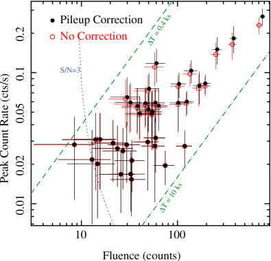
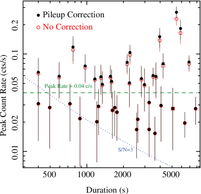
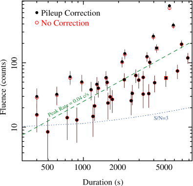
Figure 2.— Relationships between the peak count rate, fluence, and duration of the 39 flares detected during the XVP. (Top): Peak count rate and fluence, with lines marking the expected relationship for 400 s flares, 10 ks flares, and flares with S/N$=3$. (Middle): Peak count rate and duration; the gap in peak rate around 0.04 counts s${}^{-1}$ is apparent. (Bottom): Fluence and duration are strongly correlated. Squares denote flares that are truncated by the beginning/end of an observation.

4.1.2 Incompleteness and False Positives

In order to assess the incompleteness of our sample and the false positive rate, we perform a suite of Monte Carlo simulations based on our fits to the observed lightcurves. To evaluate the false positive rate, we generate 100 Poisson-random realizations of the baseline emission in each observation and search for flares. No flares are detected, which suggests that our rate of identifying background fluctuations as flares is $<1\%$, and that all of our detected flares are likely real.

We quantify our flare detection efficiency $f$ with simulations in which we inject flares, generate Poisson-random realizations, search for flares, and use the detection rate to assess the incompleteness of our sample. For each observation, we simulate 500 lightcurves with randomly placed Gaussian flares: 25 flares for each of 20 different peak count rates (logarithmically-spaced between $0.01-0.3$ counts s${}^{-1}$). To set the duration of each inserted flare, we randomly sample the observed duration distribution. When we search these simulated lightcurves, we define a flare inserted at time $t$ with width $\sigma_{t}$ as detected if our algorithm finds a flare in the time interval $t\pm 3\sigma_{t}.$ With these results we can calculate $f$ for the binned distributions (see Section 4.3). At the low end, we have $f\gtrsim 0.2-0.5;$ the incompleteness is not important for flares with fluences $\gtrsim 80$ counts or peak rates above 0.04 counts s${}^{-1}.$ To create efficiency-corrected histograms, we interpolate to find the detection efficiency at each observed flare, then take the sum of $f^{-1}$ in each bin (effectively dividing each histogram value by the average value of $f$ for the flares in that bin). We perform additional simulations to confirm (using our fluence distribution) that Poisson noise in the injected flares does not change our results to within the quoted errors.

4.2. Flare Demographics

In Figure 2, we present the relationships between the raw and pileup-corrected peak count rates, fluences, and durations of the 39 X-ray flares. We see moderate/strong correlations between the fluence of a flare and both its peak count rate (correlation coefficient $\rho\sim 0.89$) and duration ($\rho\sim 0.54$), but almost no correlation ($\rho\sim 0.27$) between the peak count rate of a flare and its duration. Pileup does not have a significant effect on these correlations.

The top panel of Figure 2, shows the peak count rate versus fluence of the Sgr A${}^{*}$ flares. Most of the flares are clustered around fluences of $\sim 60$ counts, with peak count rates in the range $0.02-0.1$ counts s${}^{-1}.$ At high fluence, the distribution of flares appears to narrow considerably. This does not appear to be an issue of incompleteness. For reference, we overplot a line representing a S/N ratio of 3, as well as lines of constant duration for single Gaussian flares with $1\sigma$ widths of 100 s (our minimum allowed width) and 2500 s, which correspond to flare durations of 400 s and 10 ks. We expect good sensitivity to flares inside this region. Thus the narrow distribution at high fluence is likely physical, and may indicate that the brightest flares have a preferred time scale ($\tau\sim 4-6$ ks). The brightest flares seen by XMM-Newton last $\sim 3$ ks (Porquet03; Porquet08), so further study is merited.

Table 2Fits to Flare Distributions

Parameter	Fluence	Peak Rate	Duration	Luminosity
Powerlaw
$N$	$67_{-34}^{+61}$	$0.75_{-0.6}^{+1.6}$	$5_{-4}^{+21}$	$50\pm 20$
$\Gamma$	$-1.5\pm 0.2$	$-1.9_{-0.5}^{+0.4}$	$-0.9\pm 0.2$	$-1.9_{-0.4}^{+0.3}$
$\chi^{2}/\nu$	8.18/5	9.7/5	3.3/5	4.6/5
Cutoff Power Law
$N$	$14_{-12}^{+44}$	$0.7_{-0.6}^{+1.2}$	$0.05_{-0.05}^{+7.6}$	$46_{-15}^{+26}$
$\Gamma$	$-0.9_{-0.5}^{+0.8}$	$-1.9_{-0.5}^{+0.8}$	$-0.1_{-0.8}^{+1.0}$	$-1.7_{-0.6}^{+1.1}$
Cutoff	$160_{-110}^{+780}$	$>0.05$	$>1500$	$>4$
$\chi^{2}/\nu$	3.8/4	9.7/4	0.8/4	4.5/4

Note. — Power law and cutoff power law fits to the distributions in Figure 3. $N$ is the power law normalization and $\Gamma$ is the power law index. Errors are 90% confidence limits for a single parameter. Errors on $N$ are typically large because they involve extrapolating outside the domain of the data.

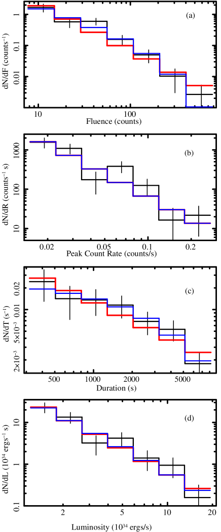
Figure 3.— Distributions of flare fluence (a), peak count rate (b), duration (c), and mean luminosity (d). In all panels, the black histograms represent distributions corrected for both pileup and our detection efficiency, with Poisson errors on the number of flares in each bin. The red curves are the best power law fit, and the blue curves are the best cutoff power law fit.

4.3. Flare Distributions

The distributions of the flare properties may also provide clues to their physical origin. In Figure 3, we present the binned differential distributions of the flare fluence, peak count rate, duration, and luminosity (all corrected for detection efficiency and for pileup; Sections 4.1.1 and 4.1.2). These are our best assessment of the intrinsic flare properties in the observed range of parameters. Assuming Poisson uncertainties on each histogram bin, a power law model provides a good fit to the distributions of durations and luminosities (red curves in Figure 3; see Table 2 for fit parameters). The luminosity distribution falls off as $dN/dL\propto L^{-1.9},$ while the duration distribution falls off as $dN/dT\propto T^{-0.9}.$ The fluence and peak rate distributions, however, are not as well described by a single power law (the best fits, $dN/dF\sim F^{-1.5}$ and $dN/dR\sim R^{-1.9}$, lead to $\chi^{2}_{\nu}\sim 1.6$ and $1.9$; see Table 2). As an alternative, we try a high-end cutoff power law, shown in blue in Figure 3. This model provides an improved fit to the fluence distribution, but not the peak rate distribution (see Section 4.3.1). Based on the properties of the brightest flare (Nowak12), the best fit fluence cutoff of $\sim 160$ counts corresponds to an absorbed $2-8$ keV fluence of $10^{-8}$ erg cm${}^{-2}$ and a total $2-10$ keV energy of $2\times 10^{38}$ erg. Although the additional parameter is clearly not required to describe the duration distribution, the best fit cutoff is about $3300$ s, which is similar to the orbital period in the inner accretion flow around Sgr A${}^{*}$. Neither of these cutoffs is well constrained.

An observational reason to prefer the models with a cutoff, however, is the absence of longer and brighter flares. For example, starting at our highest bins and integrating the best fit luminosity and duration power laws from $L=1.925\times 10^{35}$ erg s${}^{-1}$ to $L=10^{37}$ erg s${}^{-1}$ and from $T=8175$ s to $T=10^{5}$ s, we would have expected to see $3.8_{-2.8}^{+6.0}$ very luminous flares and $52_{-28}^{+48}$ very long flares if the power laws continued indefinitely. The cutoffs reduce these numbers by factors of 2.3 and 14, respectively. Presently the result is marginal, but incorporating the two dozen previously observed XMM-Newton and Chandra flares will help determine the range over which the flare properties are distributed as power laws.

4.3.1 Gaps and X-ray Colors

One reason for the poor quality of the fits to the peak count rate distribution is an apparent gap near $R\sim 0.04$ counts s${}^{-1}$ (Figure 2). The gap is also apparent as a dip in $dN/dR$ in Figure 3. Using the same scaling as in Table 1, the corresponding peak X-ray luminosity is roughly $5.4\times 10^{34}$ erg s${}^{-1}.$ There may also be a narrow gap around durations of $\sim 2$ ks that appears in the characteristic time scale (fluence divided by peak rate) of the flares, as well as the flare durations as measured by the Bayesian Blocks method (see Appendix).

These gaps are particularly interesting given our search for multiple flare populations. There are many ways to test the statistical significance of a gap in a distribution (or, alternatively, whether the distribution is bimodal). One such test is the critical bandwidth test (Silverman81; Minotte97; Hall01). The critical bandwidth $h_{\rm crit}$ is defined as the smallest smoothing parameter for which the Gaussian kernel density estimate $f_{h_{\rm crit}}$ has a single mode. The test involves drawing sample data from this kernel density distribution, finding new critical bandwidths $\hat{h}_{\rm crit}$ for the new samples, and comparing them to $h_{\rm crit}.$ In general, if the data drawn from the smoothed distribution frequently require more smoothing than the original dataset, then the distribution is likely bimodal. Quantitatively, as described by Hall01, the bimodality is significant at the level $\alpha$ if for an appropriately-chosen quantity $\lambda_{\alpha},~{}P(\hat{h}_{\rm crit}/h_{\rm crit}>\lambda_{\alpha})>1-\alpha.$

Given the large range of observed peak rates, we perform this test in log space and find that $h_{\rm crit}=0.163,$ which is $\sim 50\%$ larger than the average $1\sigma$ logarithmic uncertainty on the data. Using the Hall01 formula for $\lambda_{\alpha}(\alpha),$ we estimate that the gap in the peak rate distribution is significant at the $\sim 90\%$ level. The test does not specifically include measurement errors, but we find a similar significance level if we randomly sample the uncertainties instead of drawing new data from the kernel density distribution. Hereafter, we refer to flares above this gap as “bright” flares; those below the gap are “faint.” Although the duration gap is not significant at the 90% level in the 39 durations as reported in Table 1, it appears in the Bayesian Blocks measurements and 2 ks is a reasonable time scale for dividing “long” and “short” flares..

Table 3Flare Types and Hardness Ratios

Type	HR	Type	HR
Raw Events
Short	$1.7\pm 0.1$	Faint	$1.443\pm 0.095$
Long	$1.82\pm 0.07$	Bright	$1.92\pm 0.07$
P${}_{\rm K-S}$	0.61		$2.4\times 10^{-3}$
P${}_{\rm HR}$	0.13		$4\times 10^{-5}$
No Pileup ($1^{\rm st}$ order only)
Short	$1.0\pm 0.1$	Faint	$0.94\pm 0.08$
Long	$1.1\pm 0.06$	Bright	$1.2\pm 0.05$
P${}_{\rm K-S}$	0.45		0.13
P${}_{\rm HR}$	0.18		$4.2\times 10^{-3}$
Bkg Subtracted, No Pileup
Short	$1.27\pm 0.25$	Faint	$1.4\pm 0.3$
Long	$1.4\pm 0.1$	Bright	$1.4\pm 0.1$
P${}_{\rm HR}$	0.29		0.53

Note. — This shows the effects of pileup and contamination by diffuse X-ray emission on HR. $P_{\rm K-S}$ and $P_{\rm HR}$ are the probabilities that the two types of flare differ, as described in Section 4.3.1. The top section reports HR based on all events extracted from the zeroth and $1^{\rm st}$ orders during the flares. The middle and bottom sections use only the $1^{\rm st}$ order events to avoid pileup; we subtract an estimate of the background emission in the bottom section (see text for details). After these corrections, no significant HR variations are detected.