Phases of non-extremal multi-centered bound states

Abstract

We investigate the phase space of multi-centered near-extremal configurations previously studied in arXiv:1108.5821 Anninos:2011vn and arXiv:1110.5641 Chowdhury:2011qu in the probe limit. We confirm that in general the energetically favored ground state of the multi-center potential, which can be a single or multi-center configuration, has the most entropy and is thus thermodynamically stable. However, we find the surprising result that for a subset of configurations, even though a single center black hole seems to be energetically favored, it is entropically not allowed (the resulting black hole would violate cosmic censorship). This disproves classical intuition that everything would just fall into the black hole if energetically favored. Along the way we highlight a shortcoming in the literature regarding the computation of the angular momentum coming from electromagnetic interaction in the probe limit and rectify it. We also demonstrate that static supertubes can exist inside ergoregions where ordinary point particles would be frame dragged.

1 Introduction

Multi-centered BPS black holes Denef:2000nb ; Bates:2003vx ; Bena:2004de ; Gutowski:2004yv ; Gauntlett:2004qy ; Elvang:2004ds ; Bena:2005ni ; Bena:2005va ; Berglund:2005vb ; Saxena:2005uk and extremal non-BPS multi-centered black holes Goldstein:2008fq ; Galli:2009bj ; Bena:2009en ; Bena:2009ev ; Bena:2009fi ; Bossard:2009my ; Bossard:2009mz ; DallAgata:2010dy ; Bobev:2011kk ; Bossard:2011kz ; Bobev:2012af ; Bossard:2012xsa ; Bossard:2013oga have been known in string theory for some time. These solutions are characterized by bubble equations which determine the relative locations of the centers. For these solutions, brane probes capture the same information as the fully backreacted solution. Taking one of the centers to be a probe supertube, one finds that the minimum of the supertube potential exactly reproduces the equilibrium distance set by the supergravity bubble equations, both for BPS solutions Bena:2008dw and for certain classes of extremal non-BPS solutions Bena:2013gma .

While a lot of physics of multi-centered solutions has been understood for extremal solutions, non-extremal solutions are much richer because they radiate and are thus more realistic. Furthermore, they may shed light on important issues like the information paradox Hawking:1974sw (see Mathur:2009hf for a recent review). Dealing with full blown non-extremality is expected to be a hard problem. Instead near-extremal solutions can be studied for better control. By continuity, one would expect multi-centered solutions to exist for near-extremal systems also, albeit the minima of the potential would be lifted from the marginal value, the lifting governed by the amount of non-extremality. Indeed, such classically stable bound states were discovered in Anninos:2011vn ; Bena:2011fc ; Chowdhury:2011qu ; Bena:2012zi ; Chowdhury:2013pqa with one or several centers fully backreacted and one center treated as a probe. This kind of analysis is helpful in the context of the fuzzball proposal as well, for the construction of non-extremal microstate geometries (see Mathur:2005zp ; Bena:2004de ; Skenderis:2008qn ; Balasubramanian:2008da ; Chowdhury:2010ct for a review of the fuzzball proposal). Only a handful of very specific backreacted non-extremal solutions are known at this time Jejjala:2005yu ; Giusto:2007tt ; Bena:2009qv ; Bobev:2009kn ; see Bena:2011fc ; Bena:2012zi for new probe constructions.

We will focus on non-extremal multi-centered bound states by putting probe supertubes in non-extremal black hole backgrounds. In Chowdhury:2011qu , two of us proposed that rotating black holes will emit objects like supertubes to increase their entropy, quite like the Penrose process. It was further argued that the signature of this instability would be the minimum of the potential being lower than the value at the horizon. Such bound states were indeed found in Chowdhury:2011qu (see also Anninos:2011vn ). We demonstrate representative potentials of this kind in Figure 2.

While these findings based on the probe potential are suggestive of an interesting phase diagram, to say anything definite a careful analysis of the statistical weight of different configurations is required. This subtlety was discussed in Anninos:2011vn , but the analysis was done in the canonical ensemble. In applications where the black hole acts as a thermal bath, such that its temperature does not change during the process under consideration, the canonical ensemble is appropriate. However, when comparing stability of single center configurations towards forming multi-centered configurations and studying mergers of other centers with a black hole, the temperature of the black hole does change in general.

In this article we perform the analysis in the micro-canonical ensemble keeping energy, charges and angular momenta fixed during (de-)mergers. One subtlety that comes up when performing such an analysis is the determination of the angular momentum originating from the interaction between the electric charge of the background and the magnetic charge of the probe. The angular momentum of supertube probes in the supersymmetric BMPV black hole Breckenridge:1996is background was studied in the context of mergers in Marolf:2005cx ; Bena:2008dw , but the expressions used were incorrect as they did not transform covariantly under Lorentz transformations. We explain a correct procedure based on carefully applying the Noether method in the main body of this article, but we can already give the source of the error here. The electromagnetic angular momentum due to a magnetic monopole, $m$, and an electric point charge, $q$, located at $\vec{\rho}$ from the former can be easily found to be

$$\vec{j}=\int d^{3}r~{}\vec{r}\times(\vec{E}\times\vec{B})=-\frac{qm}{4\pi}~{}\vec{\rho}.$$ (1)

However, if one naively tries to calculate the same in the probe limit from the static Lagrangian $q\int dtA_{i}\dot{x}^{i}$ using the procedure for Noether charge, the z-component turns out to be

$$(j_{z})_{naive}=qA_{\phi}=-\frac{qm}{4\pi}(\cos\theta-k)\,,$$ (2)

which is gauge dependent through the constant $k=\pm 1$: the gauge field is ill-defined on the north or south pole of the sphere, depending on the choice of sign. Obviously, $(j_{z})_{naive}$ cannot be correct. We show the covariant procedure in the probe limit in the next section and generalize this gauge-independent procedure to extended objects. It was an implicit gauge dependence which marred the computation of angular momentum in Marolf:2005cx ; Bena:2008dw .

We also find a curious feature that the ergoregion of a supertube, the region where it cannot remain static and is dragged along an angular direction, is different from the ergoregion for point-particles. Usually, the ergoregion is thought to be a property of the background and not of the background-and-probe system. This feature applies to four-dimensional probes as well. Wrapped brane probes become charged point particles with a position dependent mass, and hence the ergoregion for such a particle can depend on the embedding coordinates of the probe and not just on the background metric.

The main result of this paper builds on the carefully derived expression for the angular momentum. We use the angular momenta of probe branes to study the phase diagrams of multi-centered configurations graphically. In the micro-canonical ensemble a dominant phase is the one with more entropy. We find that dynamical stability implies thermodynamic stability (entropic dominance) but not vice versa. What was referred to as stable bound states in our earlier work Chowdhury:2011qu , the ones with the potential at the minimum lower than that at the horizon (red curve in Figure 2(a)), are indeed stable in a thermodynamic sense. The story for the bound states at a local minimum of the probe potential that is higher than that at the horizon (green curve in Figure 2(b)) is not so straightforward. These were referred to as metastable in Chowdhury:2011qu (in a quantum tunneling sense), but to be metastable the single center configuration formed by merging the supertube with the black hole should have more entropy. We however find that while this is the case in most of the region in phase space, there are some regions where this is not true. This means that in such regions, even though from the potential it seems that the supertube would want to tunnel through the barrier to fall into the black hole, the black hole is not big enough, in a phase space sense, to accommodate it. Since the entire phase space consists of not just one or two but multi-center configurations, it is not possible to scan over all of them to say what the end point would be, but it is certainly interesting to see that while the potential makes it seem like a merger is not only possible but likely, the story is very different. We also find regions where the potential would suggest the centers would merge, but a single center is simply not allowed for the corresponding charges. This is surprising because classically it seems a black hole would absorb everything. Conversely, there are regions in which stable two center configurations exist but no corresponding black hole which would have “spat out” the supertube center.

Our results also give a glimpse of the phase space of non-extremal black holes and black rings in Taub-NUT, as our two-center solutions can be related to non-extremal three-charge black rings in Taub-NUT by spectral flow Bena:2011zw . We comment on this in the conclusion.

The plan of this paper is as follows. In Section 2 we derive the angular momentum for an extended electric probe moving in the background of a magnetic monopole. In Section 3 we use the results of the preceding section to write down the potential and angular momentum of a supertube in a Cvetic-Youm black hole. In Section 4 we demonstrate the curious feature that the ergoregion for a supertube differs from that of a point particle. In Section 5 we plot the phase space for single and two-center configurations with fixed energy, charge and angular momentum. We conclude in Section 6.

2 Angular momenta of a probe

In this section, we discuss the conserved angular momentum of a probe in a background with a magnetic field. Naively, the angular momentum depends on the background gauge potential, which is not gauge invariant. We discuss the procedure to find the correct gauge invariant conserved angular momentum. For reasons of clarity, we explain the procedure in detail for a point particle in four dimensions (inspired by PortuguCs:2009fk ), and then generalize to a $p$-brane in arbitrary spacetime dimensions.

2.1 Point particle in a magnetic field

Consider a (non-relativistic) probe particle in the background of a magnetic monopole:

$$S=\int d\tau\left(\tfrac{1}{2}M{\dot{\vec{x}}}^{2}+qA_{i}\dot{x}^{i}\right)\,,$$ (3)

with the background magnetic potential

$$A=\frac{m}{4\pi}(k-\cos\theta)d\phi\,,$$ (4)

with $m$ the magnetic monopole charge and $k=\pm 1$, depending on the gauge choice. For instance $k=1$ gives a potential that is well defined on the north pole of the $S^{2}$ spanned by $(\theta,\phi)$, and there is a Dirac string on the negative $z$-axis $(\theta=\pi)$.

Since the background magnetic field is spherically symmetric, one would expect angular momentum to be conserved. However, with the conjugate momenta $p_{i}=\partial{\cal L}/\partial\dot{x}^{i}$, the “naive angular momentum” around the $z$-axis is given by:

$$(j_{z})_{naive}=p_{\phi}=Mr^{2}\sin^{2}\theta\dot{\phi}+qA_{\phi}\,.$$ (5)

This is not covariant under rotations. Take for example a rotation around the $x$-axis, such that $\theta^{\prime}=\pi-\theta$ and $\phi^{\prime}=2\pi-\phi$. Then the gauge potential becomes

$$A^{\prime}=\frac{m}{4\pi}(-\cos\theta-k)d\phi=A(k\rightarrow-k)\,.$$ (6)

This rotates the position of the Dirac string. Of course, this is a gauge artifact and we conclude that one needs to supplement a rotation by a compensating gauge transformation to ensure that the angular momentum transforms covariantly under rotations. There are several ways to find the form of the compensating gauge transformation. One can for instance demand that the angular momentum transforms as a vector under rotations Coleman:1982cx , or one can use the angular momentum form $\vec{L}=M\vec{r}\times\dot{\vec{r}}-\frac{qm}{4\pi}\vec{r}/r$ Wu:1976ge . Another way, which we will use because of its straightforward extension to higher-dimensional probes, is to implement the gauge transformation in the Noether procedure for the construction of the angular momentum.

2.1.1 Angular momentum from Noether procedure

Under a general symmetry transformation of the embedding coordinates of the particle $x^{\prime}=x+\delta x$, the variation of the Lagrangian must be a total derivative:

$$\delta L=\frac{\partial L}{\partial x^{i}}\delta x^{i}+\frac{\partial L}{\partial\dot{x}^{i}}\frac{d\delta x^{i}}{d\tau}\equiv\frac{dK}{d\tau}\,.$$ (7)

Using the Euler-Lagrange equations, this gives the conserved charge $dQ/d\tau=0$:

$$Q=p_{i}\delta x^{i}-K\,.$$ (8)

In most applications, the contribution $K$ for the conserved charges associated to rotations is exactly zero and we find the standard expressions for the conserved (angular) momenta, as in eq. (5). For an electric particle in a magnetic field however, the contribution $K$ is exactly the necessary compensating gauge transformation of the gauge field discussed earlier.

Take a rotation with infinitesimal generator $\delta x_{I}=\xi_{I}$, where the subscript $I$ labels the rotation axis. The first term in the Lagrangian (3) is rotationally invariant. The second term gives the contribution:

$$\delta_{\xi_{I}}L=q({\cal L}_{\xi_{I}}A_{i})\,\dot{x}^{i}\equiv\frac{dK_{I}}{d\tau}\,,$$ (9)

where ${\cal L}_{\xi}$ is the Lie derivative. To see that this equation really gives the total derivative of a function $K_{I}$, remember that the potential $A$ is gauge dependent. Hence it must only be left invariant by rotations up to a gauge transformation:

$$\delta_{\xi_{I}}A_{i}={\cal L}_{\xi_{I}}A_{i}\equiv\partial_{i}\Lambda_{I}\,.$$ (10)

Therefore we find

$$K_{I}=q\Lambda_{I}\,,$$ (11)

and the conserved angular momentum charge is

$$j_{I}=\xi^{i}_{I}p_{i}-q\Lambda_{I}\,.$$ (12)

Explicitly, the generators for rotations along the three axes are:

$$\xi_{X} = -\sin\phi\frac{\partial}{\partial\theta}-\cos\phi\cot\theta\frac{\partial}{\partial\phi}\,,$$

$$\xi_{Y} = \cos\phi\frac{\partial}{\partial\theta}-\sin\phi\cot\theta\frac{\partial}{\partial\phi}\,,$$

$$\xi_{Z} = \frac{\partial}{\partial\phi}\,,$$ (13)

they satisfy $[\xi_{X},\xi_{Y}]=-\xi_{Z}$ and cyclic permutations. The associated gauge transformations are

$$\Lambda_{X} = -\frac{m}{4\pi}(k\cos\theta-1)\frac{\cos\phi}{\sin\theta}\,,$$

$$\Lambda_{Y} = -\frac{m}{4\pi}(k\cos\theta-1)\frac{\sin\phi}{\sin\theta}\,,$$

$$\Lambda_{Z} = \frac{km}{4\pi}\,.$$ (14)

Note that the condition ${\cal L}_{\xi}A_{i}=\partial_{i}\Lambda_{I}$ does not fix the constants in the gauge transformations $\Lambda_{I}$ (in particular $\Lambda_{Z}=k$). We need to impose the Poisson brackets for the $\mathop{\rm SO}(3)$ algebra of rotations:

$$\{j_{X},j_{Y}\}=-j_{Z}$$ (15)

and cyclic in $X,Y,Z$. In particular, this gives the condition

$$\xi^{i}_{X}\partial_{i}\Lambda_{Y}-\xi^{i}_{Y}\partial_{i}\Lambda_{X}=-\Lambda_{Z}\,,$$ (16)

which determines $\Lambda_{Z}$ completely. The final expression for the covariant angular momentum is then

$$j_{z}=Mr^{2}\sin^{2}\theta\dot{\phi}-\frac{qm}{4\pi}\cos\theta.$$ (17)

As a check, the static part of this expression is also obtained by integrating $(\vec{r}\times(\vec{E}\times\vec{B}))_{z}$ over all space.

2.2 Extended object in a magnetic field

We can readily extend the discussion to $p$-branes in arbitrary spacetime dimensions. The action for a probe $p$-brane with charge $q$, in a background with a $p$-form magnetic potential is:

$$S=\int d^{p+1}\sigma{\cal L}\equiv\int d^{p+1}\sigma{\cal L}_{0}+q\int C_{p+1}\,,$$ (18)

where $\sigma^{\alpha},\alpha=0,\ldots,p$ are the worldvolume coordinates, ${\cal L}_{0}$ denotes the other terms in the worldvolume action (we do not need their exact form for the present discussion) and the integral over the $(p+1)$-form is over the pullback on the $p$-brane’s worldvolume:

$$\int C_{p+1}=\int d^{p+1}\sigma\,\frac{1}{(p+1)!}C_{i_{1}\ldots i_{p+1}}\epsilon^{\alpha_{1}\ldots\alpha_{p+1}}(\partial_{\alpha_{1}}x^{i_{1}})\ldots(\partial_{\alpha_{p+1}}x^{i_{p+1}})\,.$$ (19)

Under an infinitesimal symmetry transformation of the embedding coordinates $x^{\prime}(\sigma)=x(\sigma)+\delta x(\sigma)$, the Lagrangian must be invariant up to a total derivative. This gives:

$$\delta{\cal L}=\left(\frac{\partial{\cal L}}{\partial(\partial_{\alpha}x^{i})}\frac{\partial\delta x^{i}}{\partial\sigma^{\alpha}}+\frac{\partial{\cal L}}{\partial x^{i}}\delta x^{i}\right)\equiv\partial_{\alpha}K^{\alpha}\,.$$ (20)

Using the Euler-Lagrange equations, this gives the conserved current (with $p^{\alpha}_{i}\equiv\partial\mathcal{L}/\partial(\partial_{\alpha}x^{i})$) :

$$j^{\alpha}=p^{\alpha}_{i}\delta x^{i}-K^{\alpha}\,,$$ (21)

and the conserved charge (with $d^{p}\sigma\equiv d\sigma^{1}\ldots d\sigma^{p}$):

$$Q=\int d^{p}\sigma j^{0}=\int d^{p}\sigma(p^{0}_{i}\delta x^{i}-K^{0})\,.$$ (22)

We could rewrite this in a reparametrization-invariant form, but for simplicity we will just assume that $\sigma^{0}$ is the timelike direction on the worldvolume so that we can integrate charges over surfaces of constant $\sigma^{0}$.

2.2.1 Angular momentum from Noether procedure

Consider the conserved charges for infinitesimal symmetry generators $\delta x=\xi_{I}$, labeled by $I$. We assume that the term ${\cal L}_{0}$ is invariant under the symmetry, such that only the gauge potential term transforms:

$$\delta_{I}{\cal L}=\frac{q}{(p+1)!}({\cal L}_{\xi_{I}}C_{i_{1}\ldots i_{p+1}})\epsilon^{\alpha_{1}\ldots\alpha_{p+1}}(\partial_{\alpha_{1}}x^{i_{1}})\ldots(\partial_{\alpha_{p+1}}x^{i_{p+1}})\equiv\partial_{\alpha}K^{\alpha}_{I}\,.$$ (23)

Just as for the point particle, the symmetry generators leave the gauge field invariant up to a gauge transformation:

$${\cal L}_{\xi_{I}}C_{p+1}\equiv d\Lambda^{I}\,,$$ (24)

where $\Lambda^{I}$ are $p$-forms of gauge transformations. We get

$$K^{\alpha}_{I}=\frac{q}{p!}\Lambda^{I}_{i_{1}\ldots i_{p}}\epsilon^{\alpha\alpha_{1}\ldots\alpha_{p}}(\partial_{\alpha_{1}}x^{i_{1}})\ldots(\partial_{\alpha_{p}}x^{i_{p}})\,.$$ (25)

With $\epsilon^{012\ldots p}=-1$, this gives the conserved charges:

$$Q_{I}=\int d^{p}\sigma(p_{i}^{0}\xi^{i}_{I})+q\int\Lambda^{I}\,.$$ (26)

where the second term denotes the integral of the pull-back of $\Lambda$ on the same $\sigma^{0}=cst$ surface as for the first integral.

As for the point particle, closed terms in the gauge transformations (terms for which $d\Lambda^{I}=0$) cannot be determined from (24). They can be fixed by demanding that the Poisson brackets of the conserved charges satisfy the same symmetry algebra as the Lie brackets of the symmetry generators $\xi_{A}$:

$$[\xi_{A},\xi_{B}]=f_{AB}{}^{C}\xi_{C}\,,\qquad\{Q_{A},Q_{B}\}=f_{AB}{}^{C}Q_{C}\,.$$ (27)

The non-trivial components of the Poisson brackets of the conserved charges are

$$\{Q_{A},Q_{B}\} = \int d^{p}\sigma(\xi_{A}^{i}\partial_{i}\xi_{B}^{j}-\xi_{B}^{i}\partial_{i}\xi^{A}_{j})p^{0}_{i}$$ (30)

$$+ \int d^{p}\sigma(p+1)!\,(\xi_{A}^{i}\partial_{[i}\Lambda^{B}_{i_{1}\ldots i_{p}]}-\xi_{B}^{i}\partial_{[i}\Lambda^{A}_{i_{1}\ldots i_{p}]})\left(\epsilon^{\alpha_{1}\ldots\alpha_{p}}\partial_{\alpha_{1}}x^{i_{1}}\ldots\partial_{\alpha_{p}}x^{i_{p}}\right)\,.$$

Since the first term equals $f_{AB}{}^{C}\xi^{i}_{C}p_{i}^{0}$, the Poisson bracket equations (27) give the following constraint on the gauge parameters:

$$i_{\xi_{A}}(d\Lambda_{B})-i_{\xi_{B}}(d\Lambda_{A})=f_{AB}{}^{C}(\Lambda_{C}+d\lambda_{C})\,.$$ (31)

We have allowed for an arbitrary $(p-1)$-form $\lambda_{C}$ on the right-hand side, since the gauge transformations $\Lambda$ are $p$-forms that have a “gauge invariance” themselves: $\Lambda_{C}\rightarrow\Lambda_{C}+d\lambda_{C}$; the term proportional to $d\lambda_{C}$ is a total derivative and will thus not contribute to the integral $Q_{C}$ as given in (26).

2.2.2 A String in five dimensions

Let us work this out for an example. Consider a string in five-dimensional Minkowski spacetime, with spatial coordinates:

$$x_{1}=\sin\theta\cos\phi\,, x_{3}=\cos\theta\cos\psi\,,$$

$$x_{2}=\sin\theta\sin\phi\,, x_{4}=\cos\theta\sin\psi\,,$$ (32)

and a background magnetic field

$$C_{2}=m(k-\cos^{2}\theta)d\phi\wedge d\psi\,.$$ (33)

We choose worldvolume coordinates $\sigma^{0}=\tau,\sigma^{1}=\sigma$.

We concentrate on the conserved charges for rotations in the 12 and 34 planes. From the Noether procedure, we find these are:

$$Q_{12}=\int d\sigma(p^{\tau}_{\psi}+\Lambda^{12})\,,\qquad Q_{34}=\int d\sigma(p^{\tau}_{\psi}+\Lambda^{34})\,.$$ (34)

with $d\Lambda^{12}=d\Lambda^{34}=0$. By demanding that all of the angular momentum charges obey the $SO(4)$ algebra (see Appendix A for more details),

$$\{Q_{ik},Q_{j\ell}\}=\delta_{i\ell}Q_{kj}-\delta_{k\ell}Q_{ij}+\delta_{kj}Q_{i\ell}-\delta_{ij}Q_{k\ell}\,,$$ (35)

we find the one-forms:

$$\Lambda^{12}=mk\,d\psi\,,\qquad\Lambda^{34}=m(1-k)\,d\phi\,.$$ (36)

Note that even though these one-forms satisfy are closed, $d\Lambda^{13}=d\Lambda^{34}=0$, they are not globally exact and thus not pure gauge: there is no globally well-defined $(p-1)$ form $\lambda$ which can transform them to zero as $\Lambda\rightarrow\Lambda+d\lambda$.

The gauge-independent conserved charges are then:

$$Q_{12}=Q_{12}^{0}+\int d\sigma\left(m\cos^{2}\theta\right)\partial_{\sigma}\psi\,,\qquad Q_{34}=Q_{34}^{0}+\int d\sigma\left(m\sin^{2}\theta\right)\partial_{\sigma}\phi$$ (37)

Here $Q_{ij}^{0}$ denotes the orbital angular momentum (the part coming from ${\cal L}_{0}$ in (18)).

We will make use of this result in the following section, where we consider supertubes in a non-extremal black hole background with a background magnetic field.

3 Supertube probe in a non-extremal black hole background

In this section, we give the potential and angular momenta for a supertube in the background of the five-dimensional Cvetic-Youm black hole. We use the discussion of the previous section to obtain the gauge invariant angular momenta.

3.1 Background

The Cvetic-Youm black hole Cvetic:1996xz ; Cvetic:1996kv ; Giusto:2004id is a non-extremal, rotating three charge black hole of five-dimensional supergravity. It has two angular momenta in two independent planes in $\mathbb{R}^{4}$. We give the solution in the M-theory frame where it arises from a $T^{6}$ compactification. The three charges come from M2 branes wrapped on three orthogonal $T^{2}$’s inside $T^{6}$.

The solution depends on six parameters: $m$ encodes the temperature, the three ‘boosts’ $\delta_{I}$ control the charges and $a_{1},a_{2}$ determines the angular momenta. The metric and gauge field are

$$ds_{11}^{2} = -(H_{1}H_{2}H_{3})^{-2/3}H_{m}(dt+k)^{2}+(H_{1}H_{2}H_{3})^{1/3}ds_{4}^{2}+\sum_{I=1}^{3}\frac{(H_{1}H_{2}H_{3})^{1/3}}{H_{I}}ds_{I}^{2}\,,$$

$$A_{3} = \sum_{I=1}^{3}A^{(I)}\wedge\omega_{I}\,,\qquad A^{(I)}=\coth(\delta_{I})H_{I}^{-1}(dt+k)+B^{(I)}-\coth(\delta_{I})dt\,,$$ (38)

where $ds_{I}^{2}$ and $\omega_{I}$ are the flat metric and volume form on the $I^{\rm th}$ torus. The rotation one-form $k$ and magnetic parts $B^{(I)}$ of the gauge fields are

$$k = \frac{m}{f}\left[-\frac{c_{1}c_{2}c_{3}}{H_{m}}(a_{1}\cos^{2}\theta\,d\psi+a_{2}\sin^{2}\theta\,d\phi)+s_{1}s_{2}s_{3}(a_{2}\cos^{2}\theta\,d\psi+a_{1}\sin^{2}\theta\,d\phi)\right]\,,$$

$$B^{(I)} = \frac{m}{fH_{m}}\frac{c_{J}c_{K}}{s_{I}}(a_{1}\cos^{2}\theta\,d\psi+a_{2}\sin^{2}\theta d\phi)\,,$$ (39)

with $I,J,K$ all different and we write

$$c_{I}\equiv\cosh\delta_{I}\,,\qquad s_{I}\equiv\sinh\delta_{I}\,.$$ (40)

The four-dimensional base metric is

$$ds_{4}^{2} = \frac{fr^{2}}{g}dr^{2}+f(d\theta^{2}+\sin^{2}\theta\,d\phi^{2}+\cos^{2}\theta\,d\psi^{2})$$ (41)

$$+H_{m}^{-1}(a_{1}\cos^{2}\theta\,d\psi+a_{2}\sin^{2}\theta d\phi)^{2}-(a_{2}\cos^{2}\theta\,d\psi+a_{1}\sin^{2}\theta\,d\phi)^{2}\,.$$

The solution is built from the functions

$$H_{I}=1+\frac{ms_{I}^{2}}{f}\,,\qquad H_{m}=1-\frac{m}{f}\,,\qquad f=r^{2}+a_{1}^{2}\sin^{2}\theta+a_{2}^{2}\cos^{2}\theta\,,$$

$$g=(r^{2}+a_{1}^{2})(r^{2}+a_{2}^{2})-mr^{2}\equiv(r^{2}-r^{2}_{+})(r^{2}-r^{2}_{-})\,.$$ (42)

The roots of the function $g(r)$ give the radial position of the inner and outer horizon:

$$(r_{\pm})^{2}=\frac{1}{2}\left(m-{a_{1}^{2}}-{a_{2}^{2}}\pm\sqrt{\left(m-a_{1}^{2}-a_{2}^{2}\right)^{2}-4a_{1}^{2}a_{2}^{2}}\right)\,.$$ (43)

The ADM mass, electric charges and angular momenta of the black hole are (in units where $G_{5}=\pi/4$):

$$M_{ADM} =\frac{m}{2}\sum_{I}\cosh 2\delta_{I}\,,\qquad J_{\psi}=-m(a_{1}c_{1}c_{2}c_{3}-a_{2}s_{1}s_{2}s_{3})\,,$$ (44)

$$Q_{I} =\frac{m}{2}\sinh 2\delta_{I}\,, J_{\phi}=-m(a_{2}c_{1}c_{2}c_{3}-a_{1}s_{1}s_{2}s_{3})\,.$$

There are two extremal limits. The supersymmetric extremal limit is $m,a_{1},a_{2}\rightarrow 0$ and $|\delta_{I}|\rightarrow\infty$ while keeping fixed the charges $Q_{I}$ and ratios $a_{i}/\sqrt{m}$. The four-dimensional base space becomes flat and one recovers the supersymmetric rotating three-charge BMPV black hole Breckenridge:1996is with $M_{ADM}=\sum_{I}|Q_{I}|$. In the rest of this paper, we reserve the term “supersymmetric limit” for the choice $Q_{I}>0$. The non-supersymmetric extremal limit is obtained by putting $m=(|a_{1}|+|a_{2}|)^{2}$ and has $M_{ADM}>\sum_{I}|Q_{I}|$. This is the ‘ergo-cold’ black hole studied in Dias:2007nj .

3.2 Potential and angular momentum of a supertube

We consider supertubes with the two charges $q_{1}$ and $q_{2}$ corresponding to M2 branes on the first two $T^{2}$’s. We use lower case for probe charges, upper case for background charges. The dipole charge, which we call $d_{3}$, is an M5 brane along those two $T^{2}$’s and along a one-cycle in the four-dimensional base which we parameterize by an angular coordinate $\alpha$ and two constants $b_{1},b_{2}$ describing its embedding as

$$\psi=b_{1}\alpha\,,\quad\phi=b_{2}\alpha\,.$$ (45)

The supertube potential is (see appendix B and Chowdhury:2011qu ):

$${\cal H} = \frac{1}{|d_{3}|}\frac{\sqrt{H_{m}H_{1}H_{2}H_{3}g^{(4)}_{\alpha\alpha}}}{R^{2}}\sqrt{\tilde{q}_{1}^{2}+d_{3}^{2}\frac{R^{2}}{H_{2}^{2}}}\sqrt{\tilde{q}_{2}^{2}+d_{3}^{2}\frac{R^{2}}{H_{1}^{2}}}+\frac{1}{d_{3}}\frac{H_{m}k_{\alpha}}{R^{2}}\tilde{q}_{1}\tilde{q}_{2}-d_{3}m\frac{Q_{3}}{Q_{1}Q_{2}}B^{(3)}_{\alpha}$$ (46)

$$-\coth\delta_{1}\left(\frac{\tilde{q}_{1}}{H_{1}}-q_{1}\right)-\coth\delta_{2}\left(\frac{\tilde{q}_{2}}{H_{2}}-q_{2}\right)-d_{3}\coth\delta_{1}\coth\delta_{2}\frac{k_{\alpha}}{H_{1}H_{2}}\,,$$

where $k_{\alpha},g^{(4)}_{\alpha\alpha},B^{(3)}_{\alpha}$ are the pullbacks of the rotation one-form, the four-dimensional metric (41) and the third magnetic field on the supertube worldvolume. The two kinds of charges appearing above are related as

$$\tilde{q}_{1}=q_{1}-d_{3}A_{\alpha}^{(2)}\,,\qquad\tilde{q}_{2}=q_{2}-d_{3}A_{\alpha}^{(1)}\,,$$ (47)

where $A^{(I)}_{\alpha}$ are the pullbacks of the gauge fields on the supertube worldvolume. Note that $\tilde{q}_{1}$ and $\tilde{q}_{2}$ are the brane source charges which are not conserved or quantized but $q_{1}$ and $q_{2}$ are the Page charges which are conserved and quantized (see Page:1984qv ; Chowdhury:2013pqa ; deBoer:2012ma ; Marolf:2000cb ). Thus the latter quantities will have to be kept track of when discussing supertube and black hole mergers. We have also introduced the square radius:

$$R^{2}\equiv H_{1}H_{2}H_{3}g^{(4)}_{\alpha\alpha}-H_{m}k_{\alpha}^{2}\,.$$ (48)

The angular momenta of the supertube are (see appendix B)

$$\frac{j_{i}}{T_{D4}} = \frac{1}{d_{3}}\frac{g_{\alpha i}^{(4)}k_{\alpha}-k_{i}g_{\alpha\alpha}^{(4)}}{g_{\alpha\alpha}^{(4)}}\frac{\sqrt{H_{1}H_{2}H_{3}H_{m}g_{\alpha\alpha}^{(4)}}}{R^{2}}\sqrt{\tilde{q}_{1}^{2}+d_{3}^{2}\frac{R^{2}}{H_{2}^{2}}}\sqrt{\tilde{q}_{2}^{2}+d_{3}^{2}\frac{R^{2}}{H_{1}^{2}}}$$ (49)

$$+\frac{g_{\alpha i}^{(4)}Z^{3}-k_{i}k_{\alpha}H_{m}}{R^{2}}\frac{\tilde{q}_{1}\tilde{q}_{2}}{d_{3}}+d_{3}b_{j}(-C_{ij}+\kappa_{i})+\tilde{q}_{2}A_{i}^{(2)}+q_{1}A_{i}^{(1)}\,,$$

where $i,j$ run over $\psi$, $\phi$; $k_{i}$ are the (non-pulled back) components of $k$ in (3.1), $g^{(4)}$ again stands for the 4D metric (41) and the two-form components appearing in this expression are

$$C_{\psi\phi}=-\frac{Q_{3}}{fH_{2}}\left[(r^{2}+a_{2}^{2}+ms_{2}^{2})\cos^{2}\theta-\frac{M(s_{2}^{2}-s_{1}^{2})}{fH_{1}}(a_{1}^{2}-a_{2}^{2})\cos^{2}\theta\sin^{2}\theta\right]\,,$$ (50)

We have defined the constants

$$\kappa_{\psi}=-Q_{3}\,,\qquad\kappa_{\phi}=0\,.$$ (51)

We derive the form of the angular momentum from a DBI treatment in Appendix B. The constants $\kappa_{i}$ are determined by demanding that the angular momentum charges in the flat space limit, or equivalently at spatial infinity, satisfy the $SO(4)$ algebra as discussed in Section 2. A non-trivial check of the constants $\kappa_{i}$ fixing the gauge ambiguity, is that the angular momentum is symmetric under the unphysical relabeling $(b_{1},\psi,\theta)\leftrightarrow(b_{2},\phi,\pi/2-\theta)$.

At first sight, the angular momenta do not seem to be symmetric under interchange of the tori 1 and 2 (while the Hamiltonian clearly is). However, a closer look shows that this symmetry of the supertube physics is present: the antisymmetric terms, residing solely in terms in the last line of (49), nicely cancel when expanding those terms.

3.3 Comparison with the literature

We can rearrange the angular momenta in its physically interesting components: the part along the supertube $j_{\|}$ and the part transverse to its worldvolume $j_{\perp}$:

$$j_{\|}\equiv b_{1}j_{\psi}+b_{2}j_{\phi}\,,\qquad j_{\perp}\equiv b_{1}j_{\phi}-b_{2}j_{\psi}\,.$$ (52)

The parallel component takes the particularly simple form

$$j_{\|}=\frac{q_{1}q_{2}}{d_{3}}-b_{1}b_{2}d_{3}Q_{3}\,.$$ (53)

The transverse angular momentum is not very elucidating. We only explicitly give two interesting limits. For the probe embedding we will use later, $\theta=0$ and $b_{2}=0$, only the gauge field term has a non-zero contribution, irrespective of the supertube position:

$$j_{\perp}^{(b_{2}=\theta=0)}=b_{1}j_{\phi}=b_{1}d_{3}Q_{3}\,.$$ (54)

Second, we discuss the full expression for a supersymmetric background (BMPV black hole), evaluated at the supersymmetric bound state:

$$j_{\perp}^{\rm susy}=-d_{3}Q_{3}(b_{1}^{2}\cos^{2}\theta-b_{2}^{2}\sin^{2}\theta)-\frac{q_{1}q_{2}}{d_{3}}b_{1}b_{2}(\cos^{2}\theta-\sin^{2}\theta)\,.$$ (55)

The angular momenta of a supersymmetric black hole-supertube bound state have appeared before. However, only the full backreacted solution gives the correct result. See for instance Bena:2011zw for a detailed account on the asymptotic charges of the two-center bound state. In our conventions, these are supertubes in the BMPV background with embedding $b_{1}=-b_{2}=1$, corresponding to a supertube along the Gibbons-Hawking fibre. The angular momenta are:

$$j_{\|}^{\rm susy}=d_{3}Q_{3}+\frac{q_{1}q_{2}}{d_{3}}\,,\qquad j_{\perp}^{\rm susy}=\left(-d_{3}Q_{3}+\frac{q_{1}q_{2}}{d_{3}}\right)\cos(2\theta)\,.$$ (56)

Note that $j_{\perp}^{GH}$ is the symplectic product of the charge vectors of the black hole and the supertube. For probe supertubes in supersymmetric black hole backgrounds, $j_{\perp}^{\rm susy}$ has been computed in Bena:2008dw and Marolf:2005cx without fixing the gauge ambiguity discussed in Section 2.

4 Ergoregions for supertubes different from those of point particles

In this section we demonstrate explicitly a curious feature – that the existence of an ergoregion is not just a background property, but can depend on the details of a probe in the background as well. This would make it possible for a supertube to be static inside the region where a point particle cannot be. To this end, we compare the ergoregion for probe particles to that of probe supertubes in the Cvetic-Youm background.

The black hole ergoregion is defined as the region of spacetime outside the horizon where every asymptotically timelike Killing vector becomes spacelike. For the Cvetic-Youm black hole in the M-theory frame, the relevant asymptotically timelike Killing vector is $\partial/\partial t$ and the ergoregion is

$$r_{+}<r<r_{\rm erg}(\theta)\,,$$ (57)

with $r_{+}$ the outer horizon radius and $H_{m}(r_{\rm erg}(\theta))=0$:

$$(r_{+})^{2} = \frac{1}{2}\left(m-{a_{1}^{2}}-{a_{2}^{2}}+\sqrt{\left(m-a_{1}^{2}-a_{2}^{2}\right)^{2}-4a_{1}^{2}a_{2}^{2}}\right)\,,$$

$$(r_{\rm erg})^{2} = m-a_{1}^{2}\sin^{2}\theta-a_{2}^{2}\cos^{2}\theta\,.$$ (58)

In the ergoregion, a point particle cannot be held static. If we were to insist on a static worldline, the particle’s action would be complex. The wordline action of a static point particle in a gravitational background is:

$$S_{pp}=-M\int dt\sqrt{-g_{tt}}\,.$$ (59)

so that the ergoregion is defined to be the region where $g_{tt}>0$. For a point particle in the Cvetic-Youm metric (38), this agrees with the ergoregion defined as in (57).

The supertube is an extended object; its wordvolume potential involves more metric components. The “supertube-ergoregion”, which we define as the region outside the horizon where the potential for a static supertube is not defined, can depend on the way the supertube is embedded in spacetime. The relevant term of the supertube potential (46) is:

$$\frac{1}{|d_{3}|}\frac{\sqrt{H_{m}H_{1}H_{2}H_{3}g^{(4)}_{\alpha\alpha}}}{R^{2}}\sqrt{\tilde{q}_{1}^{2}+d_{3}^{2}\frac{R^{2}}{H_{2}^{2}}}\sqrt{\tilde{q}_{2}^{2}+d_{3}^{2}\frac{R^{2}}{H_{1}^{2}}}\,.$$ (60)

The necessary condition for the potential to be real is

$$H_{m}g^{(4)}_{\alpha\alpha}\geq 0\,.$$ (61)

This condition is the analog of $H_{m}>0$ for a point particle. However, unlike the point particle, this condition depends on the embedding parameters $b_{1},b_{2}$ of the supertube through the pull-back of the metric:

$$g^{(4)}_{\alpha\alpha}=f(\sin^{2}\theta\,b_{2}^{2}+\cos^{2}\theta\,b_{1}^{2})+H_{m}^{-1}(a_{1}\cos^{2}\theta\,b_{1}+a_{2}\sin^{2}\theta\,b_{2})^{2}-(a_{2}\cos^{2}\theta\,b_{1}+a_{1}\sin^{2}\theta\,b_{2})^{2}$$ (62)

The ergoregion is then defined as

$$r_{+}<r<r_{\rm erg}(\theta,b_{1},b_{2})\,.$$ (63)

where $r_{\rm erg}$ is now the root of $H_{m}g^{(4)}_{\alpha\alpha}$. It is straightforward to see that $H_{m}g^{(4)}_{\alpha\alpha}>0$ when $H_{m}>0$; this follows immediately because the sum of the first and last terms in (62) is positive. Hence the supertube ergoregion is contained in the ergoregion of point particles. Thus, it is possible for a supertube to be static when a point particle is being frame dragged! See Figure 1 for some elucidating plots.

A similar phenomenon can occur for point particles in four-dimensional background as well, when the mass of the point particle depends on the position. A position-dependent mass is generic for wrapped brane probes. One can in principle obtain such point particles by dimensional reduction of the supertube along its worldvolume, giving a point particle in a non-extremal rotating D0-D2-D6 black hole.

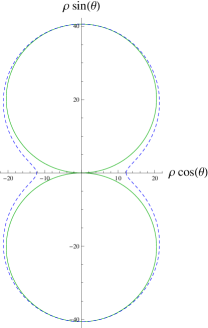
(a) $b_{1}=1,b_{2}=0$

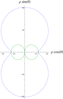
(b) $b_{1}=0,b_{2}=1$

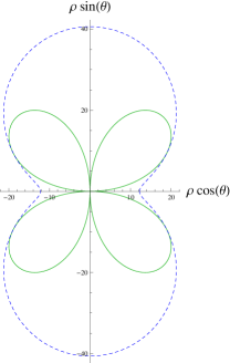
(c) $b_{1}=1,b_{2}=1$

Figure 1: Comparison of the ergoregions for point particles (blue, dashed) and supertubes (green, full) for different supertube embeddings. The background parameters used in the plots are $m=5000,a_{1}=10,a_{2}=-40$. We give the ergoregions in the $(\rho,\theta)$-plane, with $\rho=\sqrt{r^{2}-r^{2}_{+}}$ (horizon is at $\rho=0$).

5 Phase space of supertube-black hole bound states

In the supersymmetric limit, the background black hole becomes the BMPV solution and the configurations are supersymmetric two-center bound states. These were constructed in the probe limit first in Bena:2004wt ; Marolf:2005cx and the fully back-reacted solution has been known for years Bena:2008dw ; Bena:2011zw . Both the probe treatment and the supergravity back-reaction show that the supertube settles at a radius set by the ‘bubble equation’:

$$\frac{q_{1}q_{2}}{d_{3}^{2}}=H_{3}g_{\alpha\alpha}^{(4)}=\left(r^{2}+Q_{3}\right)(b_{1}^{2}\cos^{2}\theta+b_{2}^{2}\sin^{2}\theta)\,,$$ (64)

where $g_{\alpha\alpha}^{(4)}$ is the pull-back of the base space metric given (62) in the supersymmetric limit with $a_{1}\rightarrow 0,a_{2}\rightarrow 0$. As the supertubes are limits of black rings with vanishing entropy, these are toy models of rings that sit at a stable distance from the black hole. Interestingly, this configuration is also related to a pure black ring by spectral flow Bena:2011zw .

In Bena:2005zy , the authors showed that in the canonical ensemble, black rings and supertubes can be adiabatically brought to the horizon of a BMPV black hole by varying the transverse angular momentum of the supertube, $j_{\perp}$, such that the end product is again a BMPV black hole with $|J_{1}|=|J_{2}|$. This is due to a flat direction in the potential, which can extend from spatial infinity to the black hole horizon for certain charges (the bubble equation (64) allows a one-dimensional space of equilibrium separations). At non-zero temperature, the flat direction gets lifted and hence the question of moving a supertube into the black hole adiabatically is not well-posed. Therefore we pick charges such that the buble equation gives a flat direction that cannot extend into the black hole. For a non-extremal black hole, the flat direction gets lifted to an isolated minimum outside the horizon. We consider the possible transition between those bound states at isolated minima through tunneling.

In Chowdhury:2011qu , two of us studied the physics of probe supertubes for non-zero temperature, in the non-extremal Cvetic-Youm background. We showed that two-center bound states also exist when the black hole is no longer supersymmetric and has a non-zero Hawking temperature (see also Anninos:2011vn ). See Figure 2 for a few plots of the supertube potential in the non-extremal Cvetic-Youm background in five dimensions. In the plots, we normalize the potential to zero at the horizon of the black hole. Remarkably, at low temperature (low $m$, near-extremal black hole), the marginally stable supersymmetric minima can become stable: the energy of the bound state is an absolute minimum, with a lower potential value than the at the black hole horizon. As we raise the temperature, stable bound states become only local minima and eventually disappear. Very far from extremality, there are no bound states, only the black hole exists.

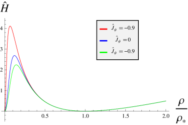
(a) Supersymmetric background ($\hat{m}=0$). Varying the background angular momentum changes the form of the potential, but not the position of the minimum.

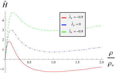
(b) Non-extremal background with $\hat{m}=1$. Generically, the supersymmetric minimum gets lifted. For an intermediate $\hat{m}$-range, local minima are possible, that can even be dynamically stable, at lower energy than the horizon value (red, solid line).

Figure 2: The supertube Hamiltonian in the black hole background. We use the embedding $b_{1}=1,b_{2}=0,\theta=0$ and the rescaled variables of section 5.3, with all charges equal $\hat{Q}\equiv\hat{Q}_{1}=\hat{Q}_{2}=\hat{Q}_{3},\,\hat{q}\equiv q_{1}=q_{2}$. We choose $\hat{d}_{3}=1$ and self-dual angular momenta $\hat{J}_{\phi}=-\hat{J}_{\psi}$ of the background. We rescaled the potential $\hat{H}={\cal H}/q$ and plot versus the radial coordinate $\rho=\sqrt{r^{2}-r^{2}_{+}}$. The horizon is at $\rho=0$. The supersymmetric minimum sits at the value $\rho=\rho_{*}\simeq 9949.87$ obtained from the bubble equation (64).

In this section, we wish to investigate these supertube-black hole bound states in more detail. We also compare the bound states of a supertube and a non-extremal black hole, with the single-center non-extremal black hole that is formed by merging the supertube with the black hole. By merger we mean the black hole that results after tunneling of the supertube from its (meta)stable position into the black hole horizon. Hence the energy, charges and angular momenta of the merged configurations are the sum of the energies, charges and angular momenta of the background and the supertube probe, where the energy and angular momentum of the probe are evaluated at the radius at which the supertube potential reaches a local minimum. We examine the parameter space of bound states and see in which regions in parameter space bound states exist and if they have more entropy than the merged black hole state.

We adopt the same terminology as in Chowdhury:2011qu . We say that the bound state is dynamically stable when the potential at the local minimum is lower than that at the horizon. When the bound state has more entropy than the single center solution we will call it thermodynamically stable. Similarly, we will say the bound state is dynamically metastable when the potential at the local minima is higher than that at the horizon and finally, when the bound state has less entropy than the single center solution we will refer to it as thermodynamically unstable.

5.1 Bound states, mergers and their entropies

The Bekenstein-Hawking entropy of the Cvetic-Youm black hole is Cvetic:1996kv

$$S_{BH}=2\pi\sqrt{(J_{+}^{\rm max})^{2}-J_{+}^{2}}+2\pi\sqrt{(J_{-}^{\rm max})^{2}-J_{-}^{2}}\,.$$ (65)

The angular momenta are:

$$J_{\pm} =\frac{J_{\phi}\pm J_{\psi}}{2}=-\frac{m}{2}(a_{2}\pm a_{1})(c_{1}c_{2}c_{3}\mp s_{1}s_{2}s_{3})\,,$$

$$J_{\pm}^{\rm max} =\frac{m^{3/2}}{2}(c_{1}c_{2}c_{3}\mp s_{1}s_{2}s_{3})\,.$$ (66)

A single-center black hole exists when there are no closed timelike curves outside the horizon, or equivalently when the entropy has no imaginary part. This happens when the angular momenta obey the “cosmic censorship bounds”:

$$|J_{\pm}|\leq|J_{\pm}^{\rm max}|\,.$$ (67)

In the supersymmetric limit $J_{-}=0$ and the bounds reduce to $|J_{+}|\leq\sqrt{Q_{1}Q_{2}Q_{3}}$.

To find the entropy of the bound state, we consider the Bekenstein-Hawking entropy of the background black hole only, since a supertube is a fundamental object without entropy. We will compare this to the entropy of the black hole that is formed after tunneling of the supertube into the background black hole. The charges of the merged state are

$$Q^{\rm tot}_{1,2}=Q_{1,2}+q_{1,2}\,,\qquad Q_{3}^{\rm tot}=Q_{3}\,,$$ (68)

and the angular momenta are

$$J_{\phi}^{\rm tot}=J_{\phi}+j_{\phi}\,,\qquad J_{\psi}^{\rm tot}=J_{\psi}+j_{\psi}\,.$$ (69)

We evaluate the supertube angular momenta $j_{i}$ at the local minimum of the supertube potential. Then the merger of the supertube and the black hole describes the black hole that results from tunneling of the supertube into the background black hole. Note that this is again a Cvetic-Youm black hole with only electric charges $Q_{I}^{\rm tot}$: since the charge $d_{3}$ of the supertube is a dipole charge, it does not contribute to the asymptotic charges of the black hole.

5.2 Parameter space

We want to understand the parameter space of black hole-supertube bound states. There are nine parameters: six for the black hole ($m,Q_{1},Q_{2},Q_{3},J_{\phi},J_{\psi}$) and three for the supertubes ($d_{3},q_{1},q_{2}$). Inspired by Anninos:2011vn we make a restriction of this parameter space to visualize the different regimes.

First we restrict to the ‘diagonal’ model, all electric charges are equal:

$$Q\equiv Q_{1}=Q_{2}=Q_{3}\,,\qquad q\equiv q_{1}=q_{2}\,.$$ (70)

Second we use the two scaling symmetries of the system. The probe potential is invariant under the two scalings $X\rightarrow\lambda_{1}^{n_{1}}\lambda_{2}^{n_{2}}X$ of the charges $X$ (see also Anninos:2011vn ):

	$m$	$Q$	$J_{i}$	$d_{3}$	$q$
$n_{1}$	2	2	3	1	2
$n_{2}$	0	0	0	1	1

The first scaling is an invariance of the equations of motion of five-dimensional $N=2$ supergravity under conformal length rescalings. It maps a background black hole solution to another black hole solution. The second one only affects the probe charges. Both scalings affect the potential by a total conformal factor and do not change the physics.

We will use the scaling symmetries to eliminate the freedom of the charges $d_{3}$ and $Q$, and define scale invariant charges as $\hat{X}=Q^{\frac{n_{2}-n_{1}}{2}}{d_{3}}^{-n_{2}}X$. In particular we choose

$$\hat{Q}=1\,,\quad\hat{m}=\frac{m}{Q}\,,\quad\hat{J}_{i}=\frac{J_{i}}{Q^{3/2}}\,,\quad\hat{d}_{3}=1\,,\quad\hat{q}=\frac{q}{d_{3}Q^{1/2}}\,.$$ (71)

This leaves us with a four-dimensional parameter space. We make two-dimensional slices of phase space by additionally fixing the ratio $J_{\phi}/J_{\psi}$ and the probe charge.

Note that the probe approximation is valid when the probe mass is small compared to the background mass: $m_{p}\ll M$. Since the ratio of these two masses has the same scaling behaviour as the ratio of the probe and background electric charges, we have:

$$\frac{m_{p}}{M}=\frac{d_{3}}{Q^{1/2}}\frac{\hat{m}_{p}}{\hat{M}}\,.$$ (72)

By making the ratio $d_{3}/Q^{1/2}$ small, we can always make sure the probe regime is valid.

5.3 Scans of parameter space

To study the existence of metastable and stable bound states, we perform a numerical scan of parameter space. We choose the probe charges and charge ratio

$$\hat{q}=10\,,$$ (73)

and the probe embedding

$$b_{1}=1\,,\qquad\ b_{2}=0\,,\qquad\theta=0\,.$$ (74)

With this choice of embedding, the local minima of the potential are at $\sin\theta=0$ due to symmetry.

The total charges are

$$Q^{\rm tot}_{1,2}=Q+q\,,\qquad Q_{3}^{\rm tot}=Q\,,$$ (75)

and the angular momenta are (see (53) and (54))

$$\hat{J}_{\phi}^{\rm tot}=\hat{J}_{\phi}+\frac{d_{3}}{Q^{1/2}}\,,\qquad\hat{J}_{\psi}^{\rm tot}=\hat{J}_{\psi}+\frac{d_{3}}{Q^{1/2}}\hat{q}^{2}\,.$$ (76)

The remaining parameter space is four-dimensional: the three rescaled variables $(\hat{m},\hat{J}_{\phi},\hat{J}_{\psi})$ and the charge ratio $d_{3}/Q^{1/2}$ that fixes the probe-to-background mass ratio (see (72)). For illustrative purposed, we only make plots of phase space for one value of this ratio. We fix:

$$d_{3}/Q^{1/2}=10^{-3}\,.$$ (77)

Other values do not change the qualitative observations. We perform two 2-dimensional slicings, one with self-dual angular momenta $J_{\phi}=-J_{\psi}$, one with $J_{\phi}=0$. The self-dual angular momenta have a well-defined supersymmetric limit $\hat{m}\rightarrow 0$ keeping the charges at fixed positive values.

5.3.1 Background with self-dual angular momenta

We first consider a background with self-dual angular momenta:

$$\hat{J}_{\phi}=-\hat{J}_{\psi}\,.$$ (78)

We examine the phase space of supertube bound states in the $(\hat{J}_{\psi},\hat{m})$-plane of the background black hole, in Figure 3(a). Note that the line $\hat{m}=0$ for $|\hat{J}_{\psi}|\leq 1$ corresponds to BMPV black holes.

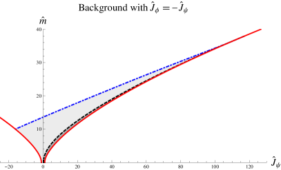
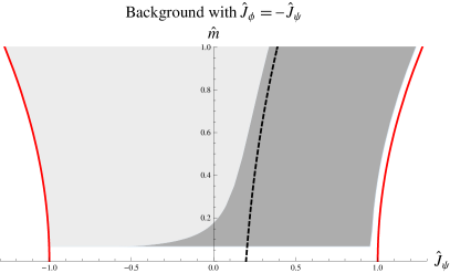
(a) Background angular momenta $J_{\psi}=-J_{\phi}$.

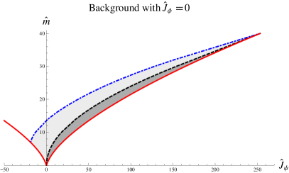
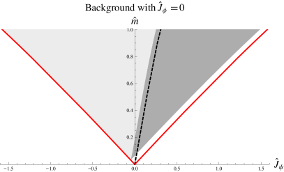
(b) Background with one angular momentum ($\hat{J}_{\phi}=0$)

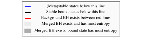
(c) Legend

Figure 3: Figure 3(a): Self-dual angular momenta of the background. The right graph is a zoom of the bottom region of the left one. The black hole background exists for given $m$ for angular momenta in between the red (solid) lines. Bound states exist between the blue (dash-dot) and the red (solid) lines. Dynamically stable bound states exist between the black (dashed) and the red (solid) lines. In the dark-grey region, the bound state has more entropy than the merger of the background black hole with the supertube (i.e. the bound state is thermodynamically stable). In the light-grey region, the merger is most entropic. Figure 3(b): The background black hole has $\hat{J}_{\phi}=0$. The right graph is a zoom of the bottom region of the left one. Bound states exist between the blue (dash-dot) and the red (solid) lines. Dynamically stable bound states exist between the black (dashed) and the red (solid) lines. In the dark-grey region, the bound state has more entropy than the merger of the background black hole with the supertube (i.e. the bound state is thermodynamically stable). In the light-grey region, the merger is most entropic.

We see that from the global picture we may conclude that thermodynamic stability goes hand in hand with dynamical stability. The boundary between the thermodynamically stable and metastable states (boundary between light-grey and dark-grey regions) follows closely the boundary between the regions in phase space with dynamically stable and dynamically metastable bound states (black, dashed line). All dynamically stable bound states are also thermodynamically stable compared to the black hole with the same total charges that describes the merger of the background with the supertube. On the other hand, most dynamically metastable states are thermodynamically unstable compared to the merged black hole.

We observe two very interesting exceptions to the general observation. The first is that right to the left of/above the black, dashed line, there is a thin dark-grey band of dynamically metastable states that are nevertheless thermodynamically stable over the merged black hole. Even though the two-center potential tells us that the supertube at the horizon has lowest energy, the larger entropy of the bound state compared to the merged state shows that the supertube and the black hole do not form a stable single-center end product for the charge configurations in this small band. It is likely that the correct end point for this set of charges is some other multi-centered configuration. However, the end point is definitely not a single center black hole.

For the second interesting exception, note that there is a small white band near the cosmic censorship bound of the background black hole (red, solid line) for positive $\hat{J}_{\psi}$ and for low background temperature (low $\hat{m}$), where the merger itself is forbidden by cosmic censorship. For dynamically metastable bound states (on the left of the black, dashed line) this result is surprising because one would expect everything to fall into a black hole. Nevertheless, the black hole cannot absorb the supertube on account of shortage of phase space. We expect that for dynamically metastable bound state in this region, there are other decays products of black holes and supertubes with other charge channels, or possibly more supertubes. For dynamically stable bound states in this region (on the right of the black, dashed line) there is no reason to expect any other phase. However, it is interesting to note that we cannot think of the supertube being “spat out” in this case as there is no corresponding single center black hole.

5.3.2 Background with rotation in one plane

We consider a background where one of the angular momenta of the background black hole is zero

$$J_{\phi}=0\,.$$ (79)

The non-zero angular momentum is then along the cycle on which the supertube is wrapped. We plot the phase space in Figure 3(b)). The findings are qualitatively the same as for a background with self-dual angular momenta. The quantitative differences are that thermodynamically stable bound states exist up to $\hat{J}_{\psi}=0$ as the background temperature goes to zero, and that the small band of dynamically metastable bounds states that are thermodynamically stable compared to the merger does not significantly widen at low $\hat{m}$.

6 Conclusions

Multi-centered black hole bound states exhibit rich physics and have been important in shedding light on various aspects of supergravity and string theory. There has been progress in the construction of multi-centered bound states in the case of non-extremal configurations recently. On the probe level, one can establish that supertubes form locally stable bound states with the non-extremal black hole Anninos:2011vn ; Bena:2011fc ; Chowdhury:2011qu ; Bena:2012zi ; Chowdhury:2013pqa , which serve as testing grounds for more intricate bound states of black holes and black rings. While the aforementioned papers studied the dynamics for a probe center around a non-extremal black hole, in this paper we went beyond dynamics to study the thermodynamics of such multi-centered solutions.

Our work confirms earlier conjectures based on the D1-D5 decoupling limit of Chowdhury:2011qu , where we compared stability and metastability of probe branes to entropies of the dual CFT states at the orbifold point. In this paper we can study entropies directly in the gravitational description that is dual to a strongly coupled CFT unlike the weakly coupled CFT at the orbifold point. We find that dynamical stability (potential at the local minimum of the supertube potential lower than that at the horizon) implies thermodynamic stability (entropic dominance of the bound state over the black hole with the same total charges). In the other direction, the connection is less strong. Dynamic metastability (potential at the local minimum of the supertube potential higher than that at the horizon) is largely synonymous with thermodynamic instability (entropic dominance of the merged state over the bound state with the same total charges). However, there is band of dynamically metastable states which are nevertheless thermodynamically stable. In addition there is another band of states, comprising both dynamically metastable and dynamically stable states, which have no corresponding merged single center black hole.

These exceptions lead us to believe that there are some dynamically metastable configurations which could tunnel into other multi-centered configurations but not single center black holes. This indicates a very rich physics for non-extremal multi-centered solutions.

Through T-dualities and spectral flow, the supertube-black hole bound states we have studied in this paper should be dual to black rings in Taub-NUT, where the charge of the ring is large compared to the Taub-NUT charge (see Bena:2011zw for this transformation in a supersymmetric setup). Hence we can ‘predict’ the existence of new non-extremal black rings in Taub-NUT space! The curious fact is that the Taub-NUT center becomes a probe in our setup. However, by playing with the ratio of probe and background charges, we can have integer charges of the probe and still be well in the probe regime.

It would be very interesting to further explore the phase space of charged multicenter bound states, similar to the phase structure of five-dimensional black holes and black rings in GR Elvang:2007hg ; Emparan:2007wm . One straightforward application is to study bound states in minimal supergravity in five dimensions (three equal M2 charges from the eleven-dimensional point of view). This is the charge setup of the four-dimensional probes used in Anninos:2011vn , the four-dimensional $t^{3}$-model. This theory has a restricted set of parameters such that it becomes possible to study phase diagrams explicitly, but it is still rich in physics. In particular, the probes in this theory are no longer supertubes. Note that there is a possible complication, since in principle the DBI action for probes in thermal backgrounds needs to be corrected as in Grignani:2010xm ; Grignani:2011mr ; Grignani:2012iw ; Armas:2012bk ; Armas:2013ota .

Methods such as the blackfold approach Emparan:2009cs ; Emparan:2009at can complement our probe approximation. As we noted above, the back-reaction of the supertube-black hole bound states of our current analysis can be related through T-dualities and spectral flow to a very massive non-extremal black ring with tree electric and three dipoles charges in Taub-NUT. Such black rings can be treated as blackfolds in a certain regime, depending on the ratio of the size of the Taub-NUT circle and the thickness of the ring horizon. To treat with such solutions of five-dimensional supergravity, the blackfold approach needs to be extended first to theories with Chern-Simons couplings of the gauge fields.

Appendix A Gauge parameters for a probe string

We write the Euclidean coordinates of four-dimensional flat space as

$$x_{1}=\sin\theta\cos\phi\,, x_{3}=\cos\theta\cos\psi\,,$$

$$x_{2}=\sin\theta\sin\phi\,, x_{4}=\cos\theta\sin\psi\,,$$ (80)

We get the following rotation generators $\xi_{ij}=x_{i}\partial_{j}-x_{j}\partial_{i}$:

$$\xi_{12} = \partial_{\phi}\,,$$

$$\xi_{34} = \partial_{\psi}\,,$$

$$\xi_{23} = -\sin\phi\cos\psi\,\partial_{\theta}-\cot\theta\cos\phi\cos\psi\,\partial_{\phi}-\tan\theta\sin\phi\sin\psi\,\partial_{\psi}\,,$$

$$\xi_{13} = -\cos\phi\cos\psi\,\partial_{\theta}+\cot\theta\sin\phi\cos\psi\,\partial_{\phi}-\tan\theta\cos\phi\sin\psi\,\partial_{\psi}\,,$$

$$\xi_{14} = -\cos\phi\sin\psi\,\partial_{\theta}+\cot\theta\sin\phi\sin\psi\,\partial_{\phi}+\tan\theta\cos\phi\cos\psi\,\partial_{\psi}\,,$$

$$\xi_{24} = -\sin\phi\sin\psi\,\partial_{\theta}-\cot\theta\cos\phi\sin\psi\,\partial_{\phi}+\tan\theta\sin\phi\cos\psi\,\partial_{\psi}\,.$$ (81)

They satisfy the $SO(4)$ algebra:

$$[\xi_{ik},\xi_{j\ell}]=\delta_{i\ell}\xi_{kj}-\delta_{k\ell}\xi_{ij}-\delta_{kj}\xi_{i\ell}-\delta_{ij}\xi_{k\ell}\,.$$ (82)

The Lie derivative of $C_{2}=m(k-\cos^{2}\theta)$ determines the exterior derivative of the gauge one-forms $\Lambda$ through (24):

$${\cal L}_{\xi_{ij}}C_{2}\equiv d\Lambda^{ij}\$$ (83)

A set of one-forms that satisfies this condition is:

$$\Lambda^{12} = -k\,d\psi\,,$$

$$\Lambda^{13} = m\sin\phi\sin\psi\,d\theta-(k+m)\cos\psi\cot\theta\sin\phi\,d\psi-k\cos\phi\sin\psi\tan\theta\,d\phi\,,$$

$$\Lambda^{14} = -m\cos\psi\sin\phi\,d\theta-(k+m)\cot\theta\sin\psi\sin\phi\,d\psi+k\cos\phi\cos\psi\tan\theta\,d\phi\,,$$

$$\Lambda^{23} = -m\cos\phi\sin\psi\,d\theta+(k+m)\cos\phi\cos\psi\cot\theta\,d\psi-k\sin\phi\sin\psi\tan\theta\,d\phi\,,$$

$$\Lambda^{24} = m\cos\phi\cos\psi\,d\theta+(k+m)\cot\theta\sin\psi\cos\phi\,\,d\psi+k\cos\psi\sin\phi\tan\theta\,d\phi\,,$$

$$\Lambda^{34} = (k+m)\,d\phi\,.$$ (84)

The arbitrary choice for $\Lambda^{12},\Lambda^{34}$ was fixed by demanding that these gauge one-forms obey the condition (31):

$$i_{\xi_{B}}d\Lambda_{A}-i_{\xi_{A}}d\Lambda_{B}=f_{AB}{}^{C}(\Lambda_{C}+d\lambda^{\prime}_{C})\,.$$ (85)

With the current choice of $\Lambda^{I}$, the gauge transformations $\lambda_{C}$ are

$$f_{AB}{}^{C}\lambda_{C}=-\frac{1}{2}(\xi_{A}^{i}\Lambda_{i}^{B}-\xi^{i}_{B}\Lambda_{A}^{i})\,.$$ (86)

The conserved charges $Q^{ij}=\xi_{ij}^{k}p_{k}+\Lambda^{ij}$ satisfy the Poisson brackets for $\mathop{\rm SO}(4)$.

Appendix B The Probe Hamiltonian and angular momentum

The procedure to find the probe Hamiltonian is very similar to that described in appendix B of Chowdhury:2011qu . We will only sketch the procedure here and highlight the differences with Chowdhury:2011qu .

B.1 Probe Lagrangian

We write the background metric as

$$ds_{11}^{2} = -(H_{1}H_{2}H_{3})^{-2/3}H_{m}(dt+k)^{2}+(H_{1}H_{2}H_{3})^{1/3}ds_{4}^{2}+\sum_{I=1}^{3}\frac{(H_{1}H_{2}H_{3})^{1/3}}{H_{I}}ds_{I}^{2},$$ (87)

and we introduce coordinates on the three torii as $(z,x_{11})$, $(y_{1},y_{2})$ and $(y_{3},y_{4})$:

$$ds_{1}^{2}=dz^{2}+dx_{11}^{2}\,,\quad ds_{2}^{2}=dy_{1}^{2}+dy_{2}^{2}\,,\quad ds_{3}^{2}=dy_{3}^{2}+dy_{4}^{2}\,.$$ (88)

The probe is a supertube, consisting of an M5-brane with dissolved M2-branes. The M5-brane wraps the coordinates of the first two $T^{2}$’s ($x_{11},z,y_{1},y_{2}$), as well as a direction in the non-compact space. Two M2-branes are dissolved in the M5, they are wrapped on torus 1 and torus 2. To find the Hamiltonian description of this M5-brane, it is easiest to first reduce to 10D type IIA supergravity on the direction $x^{11}$. The M5-brane probe becomes a D4-brane, for which the action is:

$$S_{D4} =S_{DBI}+S_{WZ},$$ (89)

$$S_{DBI} =-|N_{D4}|T_{D4}\int d^{5}\xi e^{-\Phi}\sqrt{-\det\left(g+B+F\right)},$$ (90)

$$S_{WZ} =N_{D4}T_{D4}\int d^{5}\xi\left(C_{5}+C_{3}\wedge(B+F)\right).$$ (91)

The embedding is given by $\xi^{0}\equiv\tau=t,\xi^{1}=z,\xi^{2}=\alpha,\xi^{3}=y_{1},\xi^{4}=y_{2}$ and:

$$\psi=b_{1}\alpha+v_{1}\tau\,,\quad\phi=b_{2}\alpha+v_{2}\tau\,.$$ (92)

The parameters $v_{i}$ (which are new with respect to the discussion in Chowdhury:2011qu ) determine the angular velocity of the supertube. We will set these to zero in the end since we are interested in static supertubes. They are needed to determine the angular momenta of the tube, as we will see shortly.

The metric, dilaton, NS-NS form $B_{2}$, and R-R form $C_{3}$ in 10D can be read off easily from the 11D background 38 (or from Chowdhury:2011qu ). The relevant components of $C_{5}$ can be obtained by dualizing $C_{3}$ using $dC_{5}=-*dC_{3}-H_{3}\wedge C_{3}$ (since $C_{1}=0$), and are given by:

$$C_{t\psi z12} = \frac{m\cos^{2}\theta}{fH_{1}}(a_{2}c_{1}c_{2}s_{3}-a_{1}s_{1}s_{2}c_{3})\,,$$ (93)

$$C_{t\phi z12} = \frac{m\sin^{2}\theta}{fH_{1}}(a_{1}c_{1}c_{2}s_{3}-a_{2}s_{1}s_{2}c_{3})\,,$$ (94)

$$C_{\psi\phi z12} = -\frac{Q_{3}}{fH_{2}}\left[(r^{2}+a_{2}^{2}+ms_{2}^{2})\cos^{2}\theta-\frac{m(s_{2}^{2}-s_{1}^{2})}{fH_{1}}(a_{1}^{2}-a_{2}^{2})\cos^{2}\theta\sin^{2}\theta\right]\,.$$ (95)

Finally, the world-volume field on the D4-brane is given by:

$$F=\mathcal{E}\,d\xi^{0}\wedge d\xi^{1}+\mathcal{B}\,d\xi^{1}\wedge d\alpha.$$ (96)

The electric field $\mathcal{E}$ is a source for F1 charge in the D4 worldvolume while the magnetic field $\mathcal{B}$ is a source for D2 charge.

After some algebra, one finds the Born-Infeld and Wess-Zumino Lagrangians are:

$${\cal L}_{BI} = -T_{D4}\frac{Z}{H_{2}}\Bigg{[}\frac{Z^{3}}{H_{1}^{2}}\left(Z((g_{\alpha\tau}^{(4)})^{2}-g_{\alpha\alpha}^{(4)}g_{\tau\tau}^{(4)})+\frac{H_{m}}{Z^{2}}[g_{\alpha\alpha}^{(4)}(1+k_{\tau})^{2}+k_{\alpha}(g_{\tau\tau}^{(4)}k_{\alpha}-2g_{\alpha\tau}^{(4)}(1+k_{\tau}))]\right)$$ (97)

$$\quad\qquad+\frac{H_{m}}{Z^{2}}[(1+k_{\tau})\tilde{\cal B}+k_{\alpha}\tilde{\cal E}]^{2}-Z(\tilde{\cal E}^{2}g_{\alpha\alpha}^{(4)}+2\tilde{\cal B}\tilde{\cal E}g_{\alpha\tau}^{(4)}+\tilde{\cal B}^{2}g_{\tau\tau}^{(4)})\Bigg{]}^{1/2}\,,$$

$${\cal L}_{WZ} = T_{D4}(C_{t\alpha z34}+(v_{1}b_{2}-v_{2}b_{1})C_{\psi\phi z34}-\tilde{\cal B}C_{\tau 34}-\tilde{\cal E}C_{\alpha 34})\,,$$ (98)

where we remind the reader that $g^{(4)}$ is the four-dimensional base metric (41) and $k$ the rotation one-form (3.1). The shifted electric and magnetic fields appearing in this expression are defined as

$$\tilde{\cal E}=(B+F)_{\tau z}\,,\qquad\tilde{\cal B}=(B+F)_{z\alpha}\,,$$ (99)

and the worldvolume components of the two-form and three-form fields are

$$\begin{array}[]{ll}C_{\tau 34}=A_{t}^{(2)}+v_{1}A_{\psi}^{(2)}+v_{2}A_{\phi}^{(2)}\,,&B_{\tau z}=A_{t}^{(1)}+v_{1}A_{\psi}^{(1)}+v_{2}A_{\phi}^{(1)}\,,\\ C_{\alpha 34}=A_{\alpha}^{(2)}=b_{1}A_{\psi}^{(2)}+b_{2}A_{\phi}^{(2)}\,,&B_{z\alpha}=-A_{\alpha}^{(1)}=-(b_{1}A_{\psi}^{(1)}+b_{2}A_{\phi}^{(1)})\,.\\ \end{array}$$

For later use, we give the electric field at zero velocity ($v_{i}=0$):

$$\tilde{\cal E} = \tilde{q}_{2}\frac{k_{\alpha}H_{m}}{\rho^{2}}+\tilde{q}_{1}\frac{\sqrt{H_{m}Z^{3}g_{\alpha\alpha}}}{\rho^{2}}\sqrt{\frac{\tilde{q}_{1}^{2}+\frac{\rho^{2}}{H_{2}^{2}}}{\tilde{q}_{2}^{2}+\frac{\rho^{2}}{H_{1}^{2}}}}\,,$$ (100)

with the shifted charges $\tilde{q}_{1},\tilde{q}_{2}$ defined in eq. (47).

B.2 Probe Hamiltonian

The electric field $\mathcal{E}$ is not a conserved quantity, so we need to Legendre transform the Lagrangian with respect to $\mathcal{E}$ to obtain the Hamiltonian of the tube, which will depend on the conserved charges $q_{1},q_{2}$.

The conserved F1 Page charge is given by:

$$q_{1}=\frac{\partial\mathcal{L}}{\partial\mathcal{E}}.$$ (101)

The Hamiltonian $\mathcal{H}$ is then given by:

$$\mathcal{H}=q_{1}\mathcal{E}-\mathcal{L}.$$ (102)

We further denote the D2-charge by $q_{2}$ and D4-dipole charge by $d_{3}$, so:

$$q_{2}\equiv d_{3}\mathcal{B},\qquad d_{3}\equiv N_{D4}T_{D4}\,.$$ (103)

Then, working in units where the masses of the three tori are equal to 1 (see appendix A and B of Chowdhury:2011qu for more details), and setting the angular velocity parameters $v_{1}=v_{2}=0$, we obtain the Hamiltonian given in (46).

B.3 Probe angular momentum

The background breaks rotational invariance, so there will not be a full $SO(4)$ algebra of conserved angular momenta for the supertube. However, the background (38) still has $SO(2)\times SO(2)$ symmetry generated by Killing vectors $\partial_{\phi}$ and $\partial_{\psi}$, so the angular momenta $j_{12}=j_{\phi}$ and $j_{34}=j_{\psi}$ will be conserved quantities. The angular momentum along the $x^{3}-x^{4}$ plane is given by:

$$j_{\psi}=\frac{\partial\mathcal{L}}{\partial(\partial_{\tau}\psi)}+T_{D4}d_{3}b_{2}\kappa_{1}=\frac{\partial\mathcal{L}}{\partial v_{1}}+T_{D4}d_{3}b_{2}\kappa_{\psi},$$ (104)

where we have added an a priori arbitrary constant to the quantity needed to fix the gauge ambiguity as discussed in section 2. In an analogous fashion, we have:

$$j_{\phi}=\frac{\partial\mathcal{L}}{\partial v_{2}}+T_{D4}d_{3}b_{1}\kappa_{\phi}.$$ (105)

Again, after taking the partial derivatives, we set $v_{1}=v_{2}=0$; the result is the expression (49).

At spatial infinity, rotational invariance is asymptotically realized; so all of the angular momenta of the supertube should asymptotically be conserved and satisfy the full $SO(4)$ algebra. Equivalently, we can consider the flat space limit of the background; in this limit, we again have rotational invariance and a full $SO(4)$ algebra of conserved angular momenta for the tube. For these limits, we can thus apply the reasoning of section 2 and determine the constants $\kappa_{i}$ from demanding that $j_{i}$ are the correct generators in the $SO(4)$ algebra of conserved angular momenta; this determines them to be given as in (51):

$$\kappa_{\psi}=-Q_{3}\,,\qquad\kappa_{\phi}=0\,.$$ (106)

References

- (1) D. Anninos, T. Anous, J. Barandes, F. Denef, and B. Gaasbeek, Hot Halos and Galactic Glasses, JHEP 1201 (2012) 003, [arXiv:1108.5821].
- (2) B. D. Chowdhury and B. Vercnocke, New instability of non-extremal black holes: spitting out supertubes, JHEP 1202 (2012) 116, [arXiv:1110.5641].
- (3) F. Denef, Supergravity flows and D-brane stability, JHEP 08 (2000) 050, [hep-th/0005049].
- (4) B. Bates and F. Denef, Exact solutions for supersymmetric stationary black hole composites, JHEP 1111 (2011) 127, [hep-th/0304094].
- (5) I. Bena and N. P. Warner, One ring to rule them all … and in the darkness bind them?, Adv.Theor.Math.Phys. 9 (2005) 667–701, [hep-th/0408106].
- (6) J. B. Gutowski and H. S. Reall, General supersymmetric AdS(5) black holes, JHEP 04 (2004) 048, [hep-th/0401129].
- (7) J. P. Gauntlett and J. B. Gutowski, General concentric black rings, Phys. Rev. D71 (2005) 045002, [hep-th/0408122].
- (8) H. Elvang, R. Emparan, D. Mateos, and H. S. Reall, Supersymmetric black rings and three-charge supertubes, Phys.Rev. D71 (2005) 024033, [hep-th/0408120].
- (9) I. Bena, P. Kraus, and N. P. Warner, Black rings in taub-nut, Phys. Rev. D72 (2005) 084019, [hep-th/0504142].
- (10) I. Bena and N. P. Warner, Bubbling supertubes and foaming black holes, Phys.Rev. D74 (2006) 066001, [hep-th/0505166].
- (11) P. Berglund, E. G. Gimon, and T. S. Levi, Supergravity microstates for BPS black holes and black rings, JHEP 06 (2006) 007, [hep-th/0505167].
- (12) A. Saxena, G. Potvin, S. Giusto, and A. W. Peet, Smooth geometries with four charges in four dimensions, JHEP 04 (2006) 010, [hep-th/0509214].
- (13) K. Goldstein and S. Katmadas, Almost BPS black holes, JHEP 0905 (2009) 058, [arXiv:0812.4183].
- (14) P. Galli and J. Perz, Non-supersymmetric extremal multicenter black holes with superpotentials, JHEP 1002 (2010) 102, [arXiv:0909.5185].
- (15) I. Bena, S. Giusto, C. Ruef, and N. P. Warner, Multi-Center non-BPS Black Holes - the Solution, JHEP 11 (2009) 032, [arXiv:0908.2121].
- (16) I. Bena, G. Dall’Agata, S. Giusto, C. Ruef, and N. P. Warner, Non-BPS Black Rings and Black Holes in Taub-NUT, JHEP 06 (2009) 015, [arXiv:0902.4526].
- (17) I. Bena, S. Giusto, C. Ruef, and N. P. Warner, Supergravity Solutions from Floating Branes, JHEP 1003 (2010) 047, [arXiv:0910.1860].
- (18) G. Bossard and H. Nicolai, Multi-black holes from nilpotent Lie algebra orbits, Gen.Rel.Grav. 42 (2010) 509–537, [arXiv:0906.1987].
- (19) G. Bossard, The Extremal black holes of N=4 supergravity from so(8,2+n) nilpotent orbits, Gen.Rel.Grav. 42 (2010) 539–565, [arXiv:0906.1988].
- (20) G. Dall’Agata, S. Giusto, and C. Ruef, U-duality and non-BPS solutions, JHEP 1102 (2011) 074, [arXiv:1012.4803].
- (21) N. Bobev, B. Niehoff and N. P. Warner, Hair in the Back of a Throat: Non-Supersymmetric Multi-Center Solutions from Káhler Manifolds, JHEP 1110 (2011) 149, [arXiv:1103.0520].
- (22) G. Bossard and C. Ruef, Interacting non-BPS black holes, Gen. Relativ. Gravit. (2011) [arXiv:1106.5806].
- (23) N. Bobev, B. E. Niehoff and N. P. Warner, New Supersymmetric Bubbles on , JHEP 1210 (2012) 013, [arXiv:1204.1972].
- (24) G. Bossard and S. Katmadas, Duality covariant non-BPS first order systems, JHEP 1209 (2012) 100, [arXiv:1205.5461].
- (25) G. Bossard and S. Katmadas, Duality covariant multi-centre black hole systems, arXiv:1304.6582.
- (26) I. Bena, N. Bobev, and N. P. Warner, Spectral Flow, and the Spectrum of Multi-Center Solutions, Phys.Rev. D77 (2008) 125025, [arXiv:0803.1203].
- (27) I. Bena, N. Bobev, C. Ruef, and N. P. Warner, Supertubes in Bubbling Backgrounds: Born-Infeld Meets Supergravity, JHEP 07 (2009) 106, [arXiv:0812.2942].
- (28) I. Bena, A. Puhm, O. Vasilakis, and N. P. Warner, Almost BPS but still not renormalized, arXiv:1303.0841.
- (29) S. Hawking, Particle Creation by Black Holes, Commun.Math.Phys. 43 (1975) 199–220.
- (30) S. D. Mathur, The Information paradox: A Pedagogical introduction, Class.Quant.Grav. 26 (2009) 224001, [arXiv:0909.1038].
- (31) I. Bena, A. Puhm, and B. Vercnocke, Metastable Supertubes and non-extremal Black Hole Microstates, JHEP 1204 (2012) 100, [arXiv:1109.5180].
- (32) I. Bena, A. Puhm, and B. Vercnocke, Non-extremal Black Hole Microstates: Fuzzballs of Fire or Fuzzballs of Fuzz ?, JHEP 1212 (2012) 014, [arXiv:1208.3468].
- (33) B. D. Chowdhury and D. R. Mayerson, Multi-centered D1-D5 solutions at finite B-moduli, arXiv:1305.0831.
- (34) S. D. Mathur, The fuzzball proposal for black holes: An elementary review, Fortsch. Phys. 53 (2005) 793–827, [hep-th/0502050].
- (35) K. Skenderis and M. Taylor, The fuzzball proposal for black holes, Phys. Rept. 467 (2008) 117–171, [arXiv:0804.0552].
- (36) V. Balasubramanian, J. de Boer, S. El-Showk, and I. Messamah, Black Holes as Effective Geometries, Class. Quant. Grav. 25 (2008) 214004, [arXiv:0811.0263].
- (37) B. D. Chowdhury and A. Virmani, Modave Lectures on Fuzzballs and Emission from the D1-D5 System, arXiv:1001.1444.
- (38) V. Jejjala, O. Madden, S. F. Ross, and G. Titchener, Non-supersymmetric smooth geometries and D1-D5-P bound states, Phys.Rev. D71 (2005) 124030, [hep-th/0504181].
- (39) S. Giusto, S. F. Ross, and A. Saxena, Non-supersymmetric microstates of the D1-D5-KK system, JHEP 12 (2007) 065, [arXiv:0708.3845].
- (40) I. Bena, S. Giusto, C. Ruef, and N. P. Warner, A (Running) Bolt for New Reasons, JHEP 11 (2009) 089, [arXiv:0909.2559].
- (41) N. Bobev and C. Ruef, The Nuts and Bolts of Einstein-Maxwell Solutions, JHEP 1001 (2010) 124, [arXiv:0912.0010].
- (42) J. Breckenridge, R. C. Myers, A. Peet, and C. Vafa, D-branes and spinning black holes, Phys.Lett. B391 (1997) 93–98, [hep-th/9602065].
- (43) O. J. Dias, R. Emparan, and A. Maccarrone, Microscopic theory of black hole superradiance, Phys.Rev. D77 (2008) 064018, [arXiv:0712.0791].
- (44) D. Marolf and A. Virmani, A Black hole instability in five dimensions?, JHEP 0511 (2005) 026, [hep-th/0505044].
- (45) I. Bena, B. D. Chowdhury, J. de Boer, S. El-Showk, and M. Shigemori, Moulting Black Holes, JHEP 1203 (2012) 094, [arXiv:1108.0411].
- (46) R. Portugués, Magnetic monopoles in electromagnetism and gravity, in Quantum Mechanics of Fundamental Systems: The Quest for Beauty and Simplicity (J. Zanelli and M. Henneaux, eds.), pp. 1–16. Springer New York, 2009.
- (47) S. R. Coleman, The magnetic monopole fifty years later, . In Les Houches 1981, Proceedings, Gauge Theories In High Energy Physics, Part 1, 461-552 and Harvard Univ. Cambridge - HUTP-82-A032 (82,REC.OCT.) 97p.
- (48) T. T. Wu and C. N. Yang, Dirac Monopole Without Strings: Monopole Harmonics, Nucl.Phys. B107 (1976) 365.
- (49) M. Cvetic and D. Youm, General rotating five-dimensional black holes of toroidally compactified heterotic string, Nucl.Phys. B476 (1996) 118–132, [hep-th/9603100].
- (50) M. Cvetic and D. Youm, Entropy of nonextreme charged rotating black holes in string theory, Phys.Rev. D54 (1996) 2612–2620, [hep-th/9603147].
- (51) S. Giusto, S. D. Mathur, and A. Saxena, Dual geometries for a set of 3-charge microstates, Nucl.Phys. B701 (2004) 357–379, [hep-th/0405017].
- (52) D. N. Page, CLASSICAL STABILITY OF ROUND AND SQUASHED SEVEN SPHERES IN ELEVEN-DIMENSIONAL SUPERGRAVITY, Phys.Rev. D28 (1983) 2976.
- (53) J. de Boer and M. Shigemori, Exotic Branes in String Theory, arXiv:1209.6056.
- (54) D. Marolf, Chern-Simons terms and the three notions of charge, hep-th/0006117.
- (55) V. Cardoso, O. J. Dias, and R. C. Myers, On the gravitational stability of D1-D5-P black holes, Phys.Rev. D76 (2007) 105015, [arXiv:0707.3406].
- (56) Z.-W. Chong, M. Cvetic, H. Lu, and C. Pope, Charged rotating black holes in four-dimensional gauged and ungauged supergravities, Nucl.Phys. B717 (2005) 246–271, [hep-th/0411045].
- (57) G. Gibbons, Antigravitating Black Hole Solitons with Scalar Hair in N=4 Supergravity, Nucl.Phys. B207 (1982) 337–349.
- (58) P. Galli, T. Ortin, J. Perz, and C. S. Shahbazi, Non-extremal black holes of N=2, d=4 supergravity, JHEP 1107 (2011) 041, [arXiv:1105.3311].
- (59) P. Galli, T. Ortin, J. Perz, and C. Shahbazi, Black hole solutions of N=2, d=4 supergravity with a quantum correction, in the H-FGK formalism, arXiv:1212.0303.
- (60) W. Chemissany, J. Rosseel, M. Trigiante, and T. Van Riet, The Full integration of black hole solutions to symmetric supergravity theories, Nucl.Phys. B830 (2010) 391–413, [arXiv:0903.2777].
- (61) W. Chemissany, P. Fre, J. Rosseel, A. Sorin, M. Trigiante, and T. Van Riet, Black holes in supergravity and integrability, JHEP 1009 (2010) 080, [arXiv:1007.3209].
- (62) P. Meessen, T. Ortin, J. Perz, and C. Shahbazi, H-FGK formalism for black-hole solutions of N=2, d=4 and d=5 supergravity, Phys.Lett. B709 (2012) 260–265, [arXiv:1112.3332].
- (63) I. Bena and P. Kraus, Three Charge Supertubes and Black Hole Hair, Phys. Rev. D70 (2004) 046003, [hep-th/0402144].
- (64) I. Bena, C.-W. Wang, and N. P. Warner, Sliding rings and spinning holes, JHEP 05 (2006) 075, [hep-th/0512157].
- (65) H. Elvang, R. Emparan, and P. Figueras, Phases of five-dimensional black holes, JHEP 0705 (2007) 056, [hep-th/0702111].
- (66) R. Emparan, T. Harmark, V. Niarchos, N. A. Obers, and M. J. Rodriguez, The Phase Structure of Higher-Dimensional Black Rings and Black Holes, JHEP 0710 (2007) 110, [arXiv:0708.2181].
- (67) G. Grignani, T. Harmark, A. Marini, N. A. Obers, and M. Orselli, Heating up the BIon, JHEP 1106 (2011) 058, [arXiv:1012.1494].
- (68) G. Grignani, T. Harmark, A. Marini, N. A. Obers, and M. Orselli, Thermodynamics of the hot BIon, Nucl.Phys. B851 (2011) 462–480, [arXiv:1101.1297].
- (69) G. Grignani, T. Harmark, A. Marini, N. A. Obers, and M. Orselli, Thermal string probes in AdS and finite temperature Wilson loops, JHEP 1206 (2012) 144, [arXiv:1201.4862].
- (70) J. Armas, T. Harmark, N. A. Obers, M. Orselli, and A. V. Pedersen, Thermal Giant Gravitons, JHEP 1211 (2012) 123, [arXiv:1207.2789].
- (71) J. Armas, N. A. Obers, and A. V. Pedersen, Null-Wave Giant Gravitons from Thermal Spinning Brane Probes, arXiv:1306.2633.
- (72) R. Emparan, T. Harmark, V. Niarchos, and N. A. Obers, World-Volume Effective Theory for Higher-Dimensional Black Holes, Phys.Rev.Lett. 102 (2009) 191301, [arXiv:0902.0427].
- (73) R. Emparan, T. Harmark, V. Niarchos, and N. A. Obers, Essentials of Blackfold Dynamics, JHEP 1003 (2010) 063, [arXiv:0910.1601].