Migration of massive black hole binaries in self–gravitating accretion discs: Retrograde versus prograde

Abstract

We study the interplay between mass transfer, accretion and gravitational torques onto a black hole binary migrating in a self-gravitating, retrograde circumbinary disc. A direct comparison with an identical prograde disc shows that: (i) because of the absence of resonances, the cavity size is a factor $\mathfrak{a}$(1+$\mathfrak{e}$) smaller for retrograde discs; (ii) nonetheless the shrinkage of a circular binary semi–major axis $\mathfrak{a}$  is identical in both cases; (iii) a circular binary in a retrograde disc remains circular while eccentric binaries grow more eccentric. For non-circular binaries, we measure the orbital decay rates and the eccentricity growth rates to be exponential as long as the binary orbits in the plane of its disc. Additionally, for these co-planar systems, we find that interaction ($\sim$ non–zero torque) stems only from the cavity edge plus $\mathfrak{a}$(1+$\mathfrak{e}$) in the disc, i.e. for dynamical purposes, the disc can be treated as a annulus of small radial extent. We find that simple ’dust’ models in which the binary- disc interaction is purely gravitational can account for all main numerical results, both for prograde and retrograde discs. Furthermore, we discuss the possibility of an instability occurring for highly eccentric binaries causing it to leave the disc plane, secularly tilt and converge to a prograde system. Our results suggest that there are two stable configurations for binaries in self-gravitating discs: the special circular retrograde case and an eccentric ($\mathfrak{e}$$\sim$ 0.6) prograde configuration as a stable attractor.

1 Introduction

Supermassive black hole binaries (BHBs) have been predicted to be ubiquitous intermediate products of comparable mass galaxy mergers (e.g. Begelman et al., 1980). We consider the possibility of a BHB that has migrated to reach parsec separation and is now evolving in a retrograde selfgravitating disc. Without making any a-priori statements about the astrophysical likelihood of this scenario, we compare the migration in a retrograde disc to the prograde case. Following the seminal work of Goldreich & Tremaine (1980) in the context of planetary dynamics, several studies of sub-parsec BHBs in gaseous discs (Artymowicz & Lubow, 1994; Syer & Clarke, 1995; Artymowicz & Lubow, 1996; Ivanov et al., 1999; Gould & Rix, 2000; Armitage & Natarajan, 2002, 2005; Hayasaki et al., 2007, 2008; MacFadyen & Milosavljević, 2008; Hayasaki, 2009; Cuadra et al., 2009; Haiman et al., 2009; Lodato et al., 2009; Lin & Papaloizou, 2011; Nixon et al., 2011; Roedig et al., 2011; Shi et al., 2011) employing various techniques, have established the picture sketched below. Initially the binary migrates inwards following the ’fluid elements’ of the discs (type I) migration. When the local mass of the disc (see, e.g., Kocsis et al., 2012, for a thoughtful discussion) is of the order of the mass of the lighter hole, torques exerted by the binary are strong enough to evacuate the central region of the disc carving a central cavity. Accretion continues onto both holes through the cavity. In the prograde case (studied by the aforementioned papers), the cavity itself has a radius which is about twice the binary separation, and is held up by outer Lindblad resonances. The gas at the inner edge of the circumbinary disc leaks through the cavity streaming towards either holes. The streams bend in front of each hole and are partially gravitationally captured forming minidiscs. However, a large amount of gas is flung back out impacting the disc edge, efficiently mediating the disc-binary energy and angular momentum exchange (MacFadyen & Milosavljević, 2008; Shi et al., 2011). The semi–major axis, $\mathfrak{a}$, shrinks and the eccentricity, $\mathfrak{e}$, grows and saturates around $\mathfrak{e}$$\sim$ 0.6 (Roedig et al., 2011).

Recently Nixon et al. (2011) investigated the dynamical interaction of BHB embedded in light, non-selfgravitating circumbinary retrograde discs. The absence of outer Lindblad resonances (OLR) allows the circumbinary disc to survive unperturbed outside the orbit of the binary, with the inner edge impacting directly onto the secondary BH. So, the retrograde cavity is smaller and there is neither room to accommodate large minidiscs nor will there be stream bending nor will there be sling–shots. The gas at the inner edge is either accreted directly by the secondary hole, or loses its energy and angular momentum in the impact being funneled onto the primary. We study here the evolution of BHB embedded in massive, self gravitating retrograde discs. The first goal of this paper is to compare the evolution of the orbital elements of an initially circular BHBs migrating inside pro– versus retrograde discs. The pro-retro run comparison allows us to better understand the physics of the BHB-disc interaction. We demonstrate that, in both configurations, the evolution of the binary elements is well reproduced if the BHB-disc interplay is described in terms of purely gravitational interactions, in which the gas particles are effectively treated as dust. In this picture, the hydrodynamical properties of the disc is only relevant in determining the pace at which gas is supplied for direct interaction with the BHB. At very high eccentricity we find hints of an instability that leads to the binary tilting out of the rotation plane of the disc. We pursue this possibility with a dedicated higher resolution simulation and point out the most likely cause of this behavior. Combining these finding with those of Roedig et al. (2011), we discuss that BHBs in self-gravitating retrograde discs have three possible end-stages: (1) a stable circular motion coupled with a orbit decay similar to the aligned state; depending on the stochastic occurrence of the instability either (2) a fast inspiral if the exponential eccentricity growth and semi–major axis decay bring the BHB into the gravitational wave regime or (3) re–alignment of the BHB with its disc and evolution towards the eccentric, prograde standard scenario.

The paper is organized as follows. In § 2, we describe the numerical method, initial conditions and parameters use in our simulations. In § 3, we provide a compilation of our numerical findings, that we try to explain coherently with a simple model presented in §4. The aforementioned tilting instability is studied in § 5. Concluding, we discuss and summarize the overall findings in § 6.

2 Method

Table 1: Run labels and initial parameters in code units. The prograde run is taken from paperI Roedig et al. (2012). On a side note: $N$ is the resolution, ^∗∗ denotes that additional cross–checks were preformed to ensure that all conservation laws were numerically satisfied.

Model	${\color[rgb]{0,0,1}\mathfrak{a}}_{0}$	${\color[rgb]{0,0.6,0}\mathfrak{e}}_{0}$	$r_{\rm sink}$	N	$M_{\mathrm{Disc}}/{\color[rgb]{0.5,0,1}{~{}M_{\mathrm{BHB}}}}$
$\mathtt{pro\,{\color[rgb]{0,0.6,0}\mathfrak{e}}=0}$	$1.0$	$0.02$	$0.05$	2 M	$0.186$
$\mathtt{count00}$	$0.97$	$0.02$	$0.05$	3 M	$0.13$
$\mathtt{count01}$	$0.92$	$0.09$	$0.05$	3 M	$0.13$
$\mathtt{count02}$	$0.83$	$0.19$	$0.05$	3 M	$0.13$
$\mathtt{count03}$	$0.74$	$0.30$	$0.05$	3 M	$0.13$
$\mathtt{retro\,{\color[rgb]{0,0.6,0}\mathfrak{e}}=0}$	$1.0$	$0.02$	$0.05$	2 M	$0.186$
$\mathtt{retro\,{\color[rgb]{0,0.6,0}\mathfrak{e}}=0.1}$	$1.0$	$0.10$	$0.05$	2 M	$0.186$
$\mathtt{retro\,{\color[rgb]{0,0.6,0}\mathfrak{e}}=0.3}$	$1.0$	$0.27$	$0.05$	2 M	$0.186$
$\mathtt{retro\,{\color[rgb]{0,0.6,0}\mathfrak{e}}=0.5}$	$1.0$	$0.46$	$0.05$	2 M	$0.186$
$\mathtt{retro\,{\color[rgb]{0,0.6,0}\mathfrak{e}}=0.8}$	$1.0$	$0.83$	$0.05$	2 M	$0.186$
$\mathtt{retro^{**}{\color[rgb]{0,0.6,0}\mathfrak{e}}=0.7}$	$1.0$	$0.56$	$0.05$	4 M	$0.176$
$\mathtt{retro^{**}{\color[rgb]{0,0.6,0}\mathfrak{e}}=0.9}$	$1.0$	$0.94$	$0.04$	4 M	$0.186$

The model and numerical setup of this work is closely related to that of Roedig et al. (2011, 2012)(the latter hereafter paperI) and Cuadra et al. (2009), hence we only outline the key aspects in the following, and refer the reader to these papers for further details.

We simulate a self-gravitating gaseous disc of mass $M_{\mathrm{Disc}}$ around two BHs of combined mass ${\color[rgb]{0.5,0,1}{~{}M_{\mathrm{BHB}}}}=M_{1}+M_{2}$, mass ratio $\mathfrak{q}=M_{2}/M_{1}\sim 1/3$, eccentricity ${\color[rgb]{0,0.6,0}\mathfrak{e}}$ and semi-major axis ${\color[rgb]{0,0,1}\mathfrak{a}}$, using the SPH-code Gadget-2 (Springel, 2005) in a modified version that includes sink-particles which model accreting BHs (Springel et al., 2005; Cuadra et al., 2006). The disc, which is counter-rotating with the BHs, radially extends to about $7{\color[rgb]{0,0,1}\mathfrak{a}}$, contains a circumbinary cavity of radial size $\lower 3.22916pt\hbox{$\sim$}\hbox to0.0pt{\hss\raise 1.1625pt\hbox{$>$}}{\color[rgb]{0,0,1}\mathfrak{a}}$ and is numerically resolved by at least $2$ million particles. The numerical size of each BH is denoted as $r_{\rm sink}$, the radius below which a particle is accreted, removed from the simulation, and its momentum is added to the BH (Bate et al., 1995). The gas in the disc is allowed to cool on a time scale proportional to the local dynamical time of the disc $t_{\rm dyn}=2\pi/\Omega_{0}$, where $\Omega_{0}=(\mathrm{G}M_{0}/{\color[rgb]{0,0,1}\mathfrak{a}}_{0}^{3})^{1/2}$ is the initial orbital frequency of the binary. To prevent it from fragmenting, we force the gas to cool slowly, setting $\beta=t_{\rm cool}/t_{\rm dyn}=10$ (Gammie, 2001; Rice et al., 2005). This choice of $\beta$ is discussed in previous work (e.g. paperI). All figures are shown in code units $\mathrm{G}=M_{0}=1$.

2.1 Discussion of initial conditions

We start the simulations using two different approaches for obtaining initial conditions (ICs), the relevant quantities of which are listed in Table 1. In the standard case, labeled ${\tt retro}$ throughout, a relaxed prograde disc is taken and the orbital angular momentum vector of the BHB, ${\bf L}_{\rm BHB}$, is flipped and the eccentricity is changed. To be specific, we took the ICs of model adia05 in paperI, in order to facilitate a direct prograde vs retrograde comparison. This prograde run is labeled ${\tt pro\,{\color[rgb]{0,0.6,0}\mathfrak{e}}=0}$. Additionally, to measure how fast the memory of any out-of-equilibrium IC is lost and in order to avoid any spurious systematics, the following test was performed: the cavity was filled with gas to form a solid accretion disc lacking any low density region around the BHB. A circular BHB was placed around the center of mass (CoM) and integrated to measure how many orbits the system would need to relax. We observed an initial transient marked by high accretion and BHB shrinkage that lasted $45$ orbits. Thereafter the system converged to a perfectly relaxed behavior, the evolution of which in terms of time derivative of the semi–major axis $\dot{{\color[rgb]{0,0,1}\mathfrak{a}}}$, the eccentricity $\dot{{\color[rgb]{0,0.6,0}\mathfrak{e}}}$ and mass, ${\color[rgb]{0.5,0,1}{~{}\dot{M}_{\mathrm{BHB}}}}$, could not be distinguished from the ${\tt retro\,{\color[rgb]{0,0.6,0}\mathfrak{e}}=0}$ setup. We thus only show data that exclude the first $45$ orbits, to avoid any potential initial transient. Unless otherwise stated, for each setup we use the orbits $45-90$ for the analysis.

The second set of ICs, labeled ${\tt count}$, uses a disc that was left to relax onto a retrograde, circular BHB for $750$ orbits, which is why the disc is lighter as it got depleted over time. After 750 orbits, we modify the binary semi–major axis and eccentricity, keeping the quantity $\mathfrak{a}$(1+$\mathfrak{e}$) approximately constant. This is physically motivated by the previous observation that the gap size in a prograde disc is, at zero order, determined by the apocenter of the BHB orbit. We then let the system evolve for 90 orbits and, as in the ${\tt retro}$ case, we keep orbits $45-90$ for the analysis.

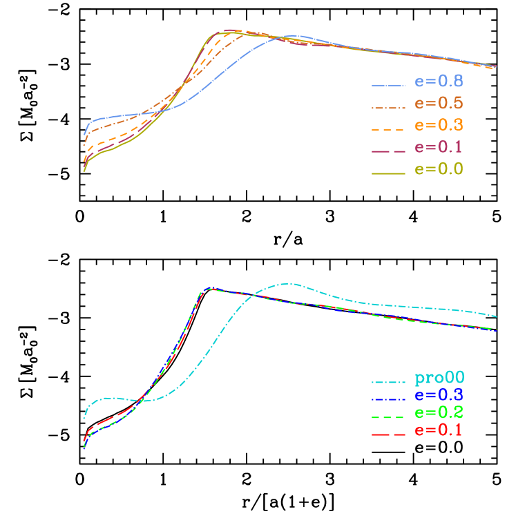
Figure 1: Retrograde runs, average surface density $\Sigma(r)$ - Top: $"{\tt retro}$ runs. Bottom: constant $(1+{\color[rgb]{0,0.6,0}\mathfrak{e}}){\color[rgb]{0,0,1}\mathfrak{a}}$ runs $"{\tt count}^{\prime\prime}$ runs, Additionally, the circular prograde case is overlayed, in which the surface density peaks at a radius that is 1 $\mathfrak{a}$  larger than in the retrograde case. Note that $M_{\mathrm{Disc}}$ in the ${\tt count}$ runs is smaller than in the ${\tt retro}$ runs. See text for more details; quantities are in code units.

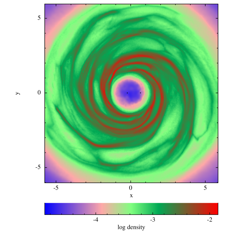
Figure 2: Disc surface density of runs ${\tt retro\,{\color[rgb]{0,0.6,0}\mathfrak{e}}=00}$ (top) and ${\tt retro\,{\color[rgb]{0,0.6,0}\mathfrak{e}}=08}$ (bottom) - Colors are in log-density scale as indicated by the colour-bars, all plots are in code units $\mathrm{G}=M_{0}={\color[rgb]{0,0,1}\mathfrak{a}}_{0}=1$ and snapshots are taken at the same time $t=70$.

In Fig. 1, we plot the surface densities of all runs (averaging over orbits $45-90$). In the top panel we show the ${\tt retro}$ profiles as a function of radius in units of $\mathfrak{a}$. As $\mathfrak{e}$  increases, the edge of the cavity is pushed outwards, and the profile of the disc inside the cavity becomes shallower. The lower panel shows the profiles of the four ${\tt count}$ setups in comparison with the prograde, circular setup, as a function of radius now in units of $\mathfrak{a}$(1+$\mathfrak{e}$). For the ${\tt count}$ runs $\Sigma(r)$ are very similar and the radial displacement in $\Sigma_{\rm max}$ between prograde and retrograde is one semi–major axis (i.e., the disc extends inwards because of lack of resonances). In Fig. 2, the logarithmic surface density inside $5{\color[rgb]{0,0,1}\mathfrak{a}}$ is shown for the two runs ${\tt retro\,{\color[rgb]{0,0.6,0}\mathfrak{e}}=0}$ and ${\tt retro\,{\color[rgb]{0,0.6,0}\mathfrak{e}}=08}$, with color code and scale identical to paperI, Fig. 9. We can appreciate here the much smaller and well defined cavity in the circular case compared to the eccentric one.

The question of the necessary resolution is addressed both by changing the total number of SPH particles and by changing the mass of each SPH particle (thus giving a different disc thickness, which must be sufficiently sampled) As can be seen by inspecting table 1, the ${\tt retro}$ runs use $2$, the ${\tt count}$ runs use $3$ and the ${\tt retro^{**}}$ runs use $4$ Million particles (where we state the resolution after discarding relaxation). We measured differential torque–densities, d$T_{{\rm G},z}/$d$r$ (see §3.2), per unit mass in ${\tt retro\,{\color[rgb]{0,0.6,0}\mathfrak{e}}=0}$ versus ${\tt count00}$, and found small, but no significant differences between the averaged torques for the circular runs. This assures us that the resolution is sufficient in the ${\tt retro}$ runs, that the results are not sensitive to the precise choice of disc mass and that the relaxation of the discs to the new BHB orbit is fast (the ${\tt count00}$ run effectively discards the first $795$ orbits of relaxation at which time it has a resolution of $3$ Million). To be conservative, we use $4$ Million particles and monitor closely all conservation laws for the more complex dynamical geometry discussed in the end of the paper.

3 Analysis of the numerical data

3.1 Binary evolution: general features

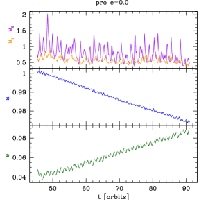
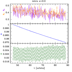
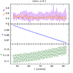
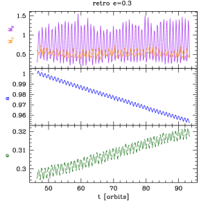
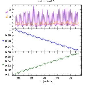
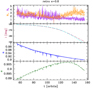
Figure 3: Evolution of the accretion rates, semi-major axis, eccentricity and inclination - All ${\tt retro}$ runs are shown, as indicated above each panel. We also show the prograde run in the top left panel. In each panel we plot the individual accretion rates $\dot{M}_{1}$, $\dot{M}_{2}$ (multiplied by $10^{5}$), the semi-major axis ${\color[rgb]{0,0,1}\mathfrak{a}}$ and the eccentricity ${\color[rgb]{0,0.6,0}\mathfrak{e}}$. In the ${\tt retro\,{\color[rgb]{0,0.6,0}\mathfrak{e}}=0.8}$ panel we also include the relative BHB-disc inclination ${\color[rgb]{0.68,0,0}\mathrm{i}}$ in degrees. Note the different scales on the $y$ axis; quantities are in code units.

We start with a qualitative description of the several outputs of the simulations. In Fig. 3, we show the measured evolution of the individual accretion rates $\dot{M}_{1}$, $\dot{M}_{2}$, semi-major axis ${\color[rgb]{0,0,1}\mathfrak{a}}$ (for clarity normalized to $\mathfrak{a}$(t=$45$)) and the eccentricity ${\color[rgb]{0,0.6,0}\mathfrak{e}}$ for all the ${\tt retro}$ runs. The circular prograde case is shown in the top left panel for comparison. For the highest $\mathfrak{e}$, we add a panel showing the inclination ${\color[rgb]{0.68,0,0}\mathrm{i}}$ in degrees; $180$°  implies perfect antialignment (an additional line shows the inclination i_2.5 of only the material inside of $r<2.5{\color[rgb]{0,0,1}\mathfrak{a}}(1+{\color[rgb]{0,0.6,0}\mathfrak{e}})$). In all cases $\langle\dot{{\color[rgb]{0,0,1}\mathfrak{a}}}\rangle<0$ (here and in the following $\langle\ast\rangle$ indicates time average) and its absolute value increases with eccentricity; i.e., more eccentric counterrotating binaries appear to shrink faster. $\langle\dot{{\color[rgb]{0,0.6,0}\mathfrak{e}}}\rangle$ is positive for ${\color[rgb]{0,0.6,0}\mathfrak{e}}>0$, but it is almost exactly zero for the quasi-circular run (${\tt retro}\,\,{\color[rgb]{0,0.6,0}\mathfrak{e}}=0$). This is in contrast to the circular prograde case, which features $\langle\dot{{\color[rgb]{0,0.6,0}\mathfrak{e}}}\rangle>0$ (top left panel). The accretion rate onto each hole is comparable in the ${\tt retro}\,\,{\color[rgb]{0,0.6,0}\mathfrak{e}}=0$ and it is smaller than the prograde case. With increasing $\mathfrak{e}$, the accretion onto the secondary hole becomes larger and highly periodic (modulated on the orbital period of the binary). The ${\tt retro}\,\,{\color[rgb]{0,0.6,0}\mathfrak{e}}=0.8$ case shows a different general behavior. The binary leaves the disc orbital plane, making accretion on the primary hole easier (the secondary hole does not ’screen’ the primary anymore) and the eccentricity growth has a turnover at $\mathfrak{e}$=0.9. We will return on this latter run extensively in §5.

3.2 Gravitational and accretion torques

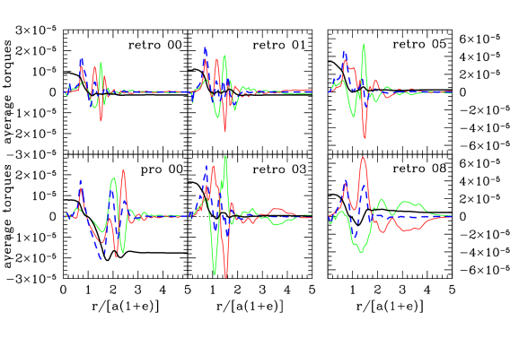
Figure 4: Gravitational torques as a function of the distance to the BHB CoM - In each panel the differential torques d$T_{{\rm G},z}/$d$r$ exerted by the disc onto the BHs are averaged over the orbits $45-90$ and shown in units of $[\mathrm{G}M^{2}_{0}({\color[rgb]{0,0,1}\mathfrak{a}}(1+{\color[rgb]{0,0.6,0}\mathfrak{e}}))^{-2}]$. We show the differential torque on the primary (red), on the secondary (green), the sum of the two (dashed–blue), and the total torques integrated inwards and outwards (black). Note that the angular momentum of the BHB is negative for retrograde runs and positive for prograde runs. See text for details.

As elucidated in paperI the evolution of the binary elements is driven by the sum of the gravitational plus the accretion torques: ${\bf\dot{L}}_{\rm BHB}={\bf T}_{\rm G}+{\bf T}_{\rm acc}$. The total gravitational torque exerted by the sum of the gaseous particles on each individual BH can be computed as

$${\bf T}_{\rm G}=\sum_{j=1}^{N}\sum_{k=1}^{2}{\bf r}_{k}\times\frac{\mathrm{G}M_{k}m_{j}({\bf r}_{j}-{\bf r}_{k})}{|{\bf r}_{j}-{\bf r}_{k}|^{3}},$$ (1)

where ${\bf r}$ is the position vector with respect to the system CoM. The accretion torque ${\bf T}_{\rm acc}$ is measured from the conservation of linear momentum in the accretion process of each particle, i.e, ${\bf T}_{\rm acc}={\bf r}_{k}\times m_{j}{\bf v}_{j}$ (here ${\bf r}_{k}$ is the position vector of the accreting BH, and $m_{j}$ and ${\bf v}_{j}$ are the mass and velocity of the accreted gas particle). In the following, all torques are averaged both in time and azimuth. In all ${\tt retro}$ runs, we use a reference frame in which the angular momentum of the disc, ${\bf L_{\rm disc}}$, is initially aligned to the $z$ axis and points in the positive $z$-direction, whereas ${\bf L_{\rm BHB}}$ points in the negative $z$-direction. Assuming that the binary and the disc are coplanar, the system is effective two-dimensional from the dynamical standpoint. We can therefore safely take ${\bf L}\approx L_{z}$ and ${\bf T}\approx T_{z}$, and unless otherwise specified, we will always refer to the $z$ components of these quantities.

As discussed in the previous section, the natural scale of the system is the apocenter distance of the BHB. We thus integrate the differential torques both in– and outwards of ${\color[rgb]{0,0,1}\mathfrak{a}}(1+{\color[rgb]{0,0.6,0}\mathfrak{e}})$ as:

$$\langle T_{z,[a,b]}\rangle=\left\langle\int_{a}^{b}\frac{dT_{z}}{dr}dr\right\rangle,$$ (2)

In Fig. 4, we show the differential, gravitational torque d$T_{{\rm G},z}/$d$r$ on the primary BH (red), on the secondary BH (green), the sum of the two (blue), and the total integrated torque (black). In opposition to the prograde case, the figure clarifies that the interaction between the disc and the binary takes place mostly at the location of the secondary, supporting a direct ’BH-gas impact’ model, as described by Nixon et al. (2011). The differential torque density, d$T_{{\rm G},z}/$d$r$ , of the runs ${\tt pro\,{\color[rgb]{0,0.6,0}\mathfrak{e}}=0}$ and ${\tt retro\,{\color[rgb]{0,0.6,0}\mathfrak{e}}=0}$ is shown in Fig. 5, where the leftmost panels show the total d$T_{{\rm G},z}/$d$r$ on the binary, the middle panel the torque density onto the primary BH and the right, onto the secondary BH. Here, we can clearly appreciate the absence of a gap between $\mathfrak{a}$  and 2$\mathfrak{a}$  in the retrograde run. The lower left panel highlights the unbalanced positive torque (blue) at the location of the secondary hole, which is responsible for the binary evolution (Note, that the orbital angular momentum of the binary is negative in the $\tt retro$ runs).

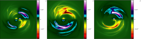
Figure 5: Gravitational torque density - Differential torque density in the $z$-direction for two initially circular BHB runs after $70$ orbits. Top (bottom) panels: ${\tt pro\,{\color[rgb]{0,0.6,0}\mathfrak{e}}=0}$ (${\tt retro\,{\color[rgb]{0,0.6,0}\mathfrak{e}}=0}$). In each row, from left to right we show the total torque density on the binary $T_{{\rm G},z}=M_{1}\,T_{{\rm G},z_{1}}+M_{2}\,T_{{\rm G},z_{2}}$, the torque onto the primary BH, $T_{{\rm G},z_{1}}$, and the torque onto the secondary BH, $T_{{\rm G},z_{2}}$. Figure made using SPLASH (Price, 2007).

Differentiating ${\bf L_{\rm BHB}}$ with respect to the relevant binary elements, angular momentum conservation yields:

$$\frac{\dot{{\color[rgb]{0,0,1}\mathfrak{a}}}}{{\color[rgb]{0,0,1}\mathfrak{a}}}={\color[rgb]{0,0.44,0.57}\frac{2\,T_{\rm G_{z}}}{L_{z}}}+{\color[rgb]{0.68,0,0}\frac{2\,T_{\rm acc_{z}}}{L_{z}}}-\frac{\dot{{\color[rgb]{1,0,0}M}}}{{\color[rgb]{1,0,0}M}}-\frac{{\color[rgb]{1,0.39,0.13}2}\dot{{\color[rgb]{1,0.39,0.13}\mu}}}{{\color[rgb]{1,0.39,0.13}\mu}}+{\color[rgb]{0,0.6,0}\frac{2{\color[rgb]{0,0.6,0}\mathfrak{e}}}{1-{\color[rgb]{0,0.6,0}\mathfrak{e}}^{2}}\dot{{\color[rgb]{0,0.6,0}\mathfrak{e}}}},$$ (3)

where ${\color[rgb]{1,0.39,0.13}\mu}=M_{1}M_{2}/M$ is the binary reduced mass. Note that all quantities in Eq. (3) can be directly measured from the simulation outputs. We can therefore use it to get an empirical measurement on how the angular momentum exchange is redistributed among the relevant binary elements. We have cast Eq. (3) in terms of the shrinkage rate and show in Fig. 7 that the two major contributions are ${\color[rgb]{0,0.44,0.57}\frac{2\,T_{\rm G_{z}}}{L_{z}}}$ and ${\color[rgb]{0,0.6,0}\frac{2{\color[rgb]{0,0.6,0}\mathfrak{e}}}{1-{\color[rgb]{0,0.6,0}\mathfrak{e}}^{2}}\dot{{\color[rgb]{0,0.6,0}\mathfrak{e}}}}$ which are of opposite sign and intrinsically coupled with each other. From this decomposition (cast in terms of the orbital element of choice) we can get a heuristic understanding of the BHB-disc coupling, which will serve as a guide for an analytical interpretation of the results.

3.3 Comparison of circular runs: prograde vs retrograde phenomenology

As we chose the setup of the ${\tt retro}$ runs to be the same as those of the adia05 run of paperI, we can compare the evolution of $\mathfrak{a}$  and $\mathfrak{e}$  directly. In Fig. 6, we thus plot the circular runs $\mathtt{retro\,{\color[rgb]{0,0.6,0}\mathfrak{e}}=0}$ vs ${\tt pro\,{\color[rgb]{0,0.6,0}\mathfrak{e}}=0}$. The evolution of $\mathfrak{a}$  is not distinguishable over the $45$ orbits that we show; on the other hand, the eccentricity behavior is different, such that $\dot{{\color[rgb]{0,0.6,0}\mathfrak{e}}}|_{\rm retro}=0$ whereas $\dot{{\color[rgb]{0,0.6,0}\mathfrak{e}}}|_{\rm pro}>0$. Upon inspecting Fig. 3, we find that also the accretion rates for the prograde setup are larger and that while the individual rates are equal for the retrograde, the secondary BH accretes and varies more in the prograde.

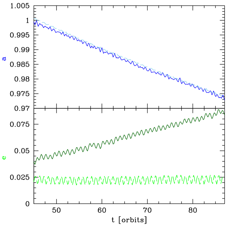
Figure 6: Evolution of semi major axis and eccentricity for circular BHBs - Direct comparison of the prograde (solid lines) and retrograde (dashed lines) systems. Only the stage after the initial transient is shown. The evolution of $\mathfrak{a}$  cannot be distinguished between the two setups, whereas the evolution of $\mathfrak{e}$  is substantially different.

Considering now the very left panels of Fig. 4, focusing only on the gravitational inwards torque, $T_{{\rm in},z}$, we find them to be very similar, but opposite in sign with respect to $L_{{\rm BHB},z}$. However, the integrated $T_{{\rm in},z}$ is slightly smaller in the prograde and there are three clear differences:

1. the radial location of largest (differential) torque amplitude onto the individual holes are displaced by a factor $\mathfrak{a}$ ;

2. the largest peak of the (differential) torque onto the binary (blue dashed line) is around $r\sim 1.7{\color[rgb]{0,0,1}\mathfrak{a}}(1+{\color[rgb]{0,0.6,0}\mathfrak{e}})$, (coinciding with the first OLR) where the torques onto the individual holes are in phase, is absent in the retrograde case;

3. the substantial outwards torques found in the prograde case are completely absent in the retrograde case;

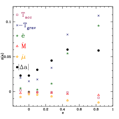
Figure 7: Contributions to $\dot{{\color[rgb]{0,0,1}\mathfrak{a}}}$ by individual components; the ${\tt pro00}$ run is inserted as negative $\mathfrak{e}$. Terms color–coded according to Eq. 3.

Note that, integrated across the whole $r$ range, the total torques on the binary always have opposite sign with respect to the orientation of L_BHB, causing a net transfer of angular momentum from the binary to the disc both in the prograde and in the retrograde case. Turning to the redistribution of the angular momentum transfer among the binary elements as detailed by equation (3), we show the individual terms from the perspective of $\dot{{\color[rgb]{0,0,1}\mathfrak{a}}}$ in Fig. 7 and first compare the two leftmost (i.e. circular) runs. We observe that

1. the contribution of ${\color[rgb]{0,0.6,0}\frac{2{\color[rgb]{0,0.6,0}\mathfrak{e}}}{1-{\color[rgb]{0,0.6,0}\mathfrak{e}}^{2}}\dot{{\color[rgb]{0,0.6,0}\mathfrak{e}}}}$ (filled pentagons) is negligible for the retrograde as $\dot{{\color[rgb]{0,0.6,0}\mathfrak{e}}}=0$

2. $2\,T_{{\rm acc},z}/L_{z}$ (open squares) contributes negatively for the retrograde, whereas positively (and three times stronger) for the prograde. The sign simply reflects the sign of $L_{z}$.

3. the mass transfer factors ${\color[rgb]{1,0.39,0.13}2}\,\dot{{\color[rgb]{1,0.39,0.13}\mu}}/{\color[rgb]{1,0.39,0.13}\mu}$ and ${\color[rgb]{1,0,0}\dot{M}/M}$ are larger by a factor $\sim$ 2 in the prograde case.

4. summing up all components gives a very similar $\dot{{\color[rgb]{0,0,1}\mathfrak{a}}}$

Taken together, these points show that for the retrograde case, the gravitational torque is indeed directly related to the binary semi–major axis evolution, given that the distribution of angular momentum among the other elements of the binary (mass, mass ratio and eccentricity) is negligible.

3.4 Eccentric runs

We turn now to the description of the phenomenology of eccentric runs. In the following, we provide some analytical fits to the few measured data points provided by our set of 5 simulations ({${\tt retro\,{\color[rgb]{0,0.6,0}\mathfrak{e}}=0\,{\color[rgb]{0,0.6,0}\mathfrak{e}}=0.1\,{\color[rgb]{0,0.6,0}\mathfrak{e}}=0.3\,{\color[rgb]{0,0.6,0}\mathfrak{e}}=0.5\,{\color[rgb]{0,0.6,0}\mathfrak{e}}=0.8}$}). We note that sometimes either the circular or the tilting run (${\tt{\color[rgb]{0,0.6,0}\mathfrak{e}}=0.8}$) had to be excluded, and we caution that the fitting functions have only few degree of freedom less than the number of sample points, which is why we do not pursue any extrapolation or other use of the numerical fit-coefficients.

In Fig. 4, we plot the evolution of the torque structure from circular to eccentric, and in Fig. 7 the contributions to the shrinkage rate, $\dot{{\color[rgb]{0,0,1}\mathfrak{a}}}$ are given, also using the total integrated torque components. Clear trends with increasing $\mathfrak{e}$  are:

1. with the exception of the run ${\tt retro\,{\color[rgb]{0,0.6,0}\mathfrak{e}}=0.8}$, the integrated inward torque grows with $\mathfrak{e}$  as

   $$T_{{\rm in},z}({\color[rgb]{0,0.6,0}\mathfrak{e}})\approx T_{{\rm in},z}({\color[rgb]{0,0.6,0}\mathfrak{e}}=0)+10\cdot T_{{\rm in},z}({\color[rgb]{0,0.6,0}\mathfrak{e}}=0)\,{\color[rgb]{0,0.6,0}\mathfrak{e}}^{2};$$ (4)

2. the integrated outward torque grows linearly with $\mathfrak{e}$ , for ${\color[rgb]{0,0.6,0}\mathfrak{e}}\neq 0$, but is always negligible with respect to the inward torque;

3. a positive bump appears in the outward torque around $r\sim 1.5{\color[rgb]{0,0,1}\mathfrak{a}}(1+{\color[rgb]{0,0.6,0}\mathfrak{e}})$, for ${\color[rgb]{0,0.6,0}\mathfrak{e}}\neq 0$;

4. the amplitude of the differential torques, d$T_{{\rm G},z}/$d$r$ , grows with $\mathfrak{e}$;

5. the maximum radius outside of which d$T_{{\rm G},z}/$d$r$ $\sim 0$ is approximately $r_{\rm max}\lower 3.22916pt\hbox{$\sim$}\hbox to0.0pt{\hss\raise 1.1625pt\hbox{$<$}}2.5{\color[rgb]{0,0,1}\mathfrak{a}}(1+{\color[rgb]{0,0.6,0}\mathfrak{e}})$ (cf. dashed blue lines).

6. ${\tt retro\,{\color[rgb]{0,0.6,0}\mathfrak{e}}=0.8}$ shows a qualitatively different torque structure, namely there is a large differential torque outside of $r={\color[rgb]{0,0,1}\mathfrak{a}}(1+{\color[rgb]{0,0.6,0}\mathfrak{e}})$, there is a high and positive net torque resulting from the fact, that now pairs of two subsequent individual, differential torques (either red or green) alternate in sign, rather than single peaks alternating after every extreme (all other panels). We conjecture, that this reflects the BHB leaving the plane of the disc; an effect that will be discussed further in § 5.

Measuring the derivatives of the orbital elements as a function of $\mathfrak{e}$, we additionally find (cf. Figs 8 and 9):

• the dependence of $\dot{{\color[rgb]{0,0.6,0}\mathfrak{e}}}({\color[rgb]{0,0.6,0}\mathfrak{e}})$ (as long as the inclination stays zero) is linear and positive:

  $$\dot{{\color[rgb]{0,0.6,0}\mathfrak{e}}}({\color[rgb]{0,0.6,0}\mathfrak{e}})\approx-0.0034+0.09\,{\color[rgb]{0,0.6,0}\mathfrak{e}}$$ (5)

  implying a threshold eccentricity of ${\color[rgb]{0,0.6,0}\mathfrak{e}}\sim 0.04$, for where the growth of $\mathfrak{e}$  would be excited;

• the dependence of $\dot{{\color[rgb]{0,0,1}\mathfrak{a}}}({\color[rgb]{0,0.6,0}\mathfrak{e}})$ is linear and negative;

• the dependence of ${\color[rgb]{0.5,0,1}{~{}\dot{M}_{\mathrm{BHB}}}}({\color[rgb]{0,0.6,0}\mathfrak{e}})$ is linear and positive;

• the dependence of ${{\color[rgb]{0.25,0.1,1}\dot{M}_{2}}}/{{\color[rgb]{1,.5,0}\dot{M}_{1}}}({\color[rgb]{0,0.6,0}\mathfrak{e}})$ is a concave parabola with a best fit maximum around ${\color[rgb]{0,0.6,0}\mathfrak{e}}\sim 0.43$;

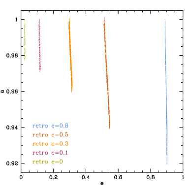
Figure 8: Semi–major axis $\mathfrak{a}$ , and eccentricity $\mathfrak{e}$  evolution in the retro runs. All runs cover the same time interval. See text for details.

3.5 Accretion rates

In Fig. 3, we can spot clear trends in both ${\color[rgb]{0.5,0,1}{~{}\dot{M}_{\mathrm{BHB}}}}$ and ${{\color[rgb]{0.25,0.1,1}\dot{M}_{2}}}/{{\color[rgb]{1,.5,0}\dot{M}_{1}}}$ with ${\color[rgb]{0,0.6,0}\mathfrak{e}}$. We explore this further in Fig. 9, where we show the accretion rates, both their sum and their ratio, as a function of eccentricity. The combined accretion rate increases with increasing ${\color[rgb]{0,0.6,0}\mathfrak{e}}$, in contrast to what was observed for prograde discs in paperI. The explanation is straightforward: for prograde runs the cavity is forced to expand with higher ${\color[rgb]{0,0.6,0}\mathfrak{e}}$ due to resonances and slingshots whereas this is not the case for retrograde runs where instead the binary penetrates further and into the disc edge and thus accretes more. Note also that the accretion rate growth is proportional to the enhancement of the inwards torque in Fig. 4 (with the exception of the ${\tt retro\,{\color[rgb]{0,0.6,0}\mathfrak{e}}=0.8}$ case), establishing a clear link between the two quantities. The ratio of secondary to primary accretion rate reaches a maximum somewhere in the range $0.4<{\color[rgb]{0,0.6,0}\mathfrak{e}}<0.6$ and declines for higher ${\color[rgb]{0,0.6,0}\mathfrak{e}}$. Conversely, in the prograde case (Roedig et al., 2011), the ratio decreases to around ${{\color[rgb]{0.25,0.1,1}\dot{M}_{2}}}/{{\color[rgb]{1,.5,0}\dot{M}_{1}}}\sim 1$ only for very high ${\color[rgb]{0,0.6,0}\mathfrak{e}}\sim 0.8$ and there is no turnover.

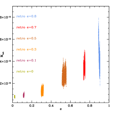
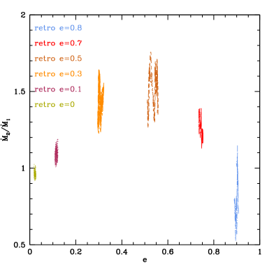
Figure 9: Mass transfer rates as function of eccentricity - (Top): Total accretion rate for the different runs. (Bottom): ratio between secondary and primary accretion rate $\dot{M_{2}}/\dot{M_{1}}$, as a function of eccentricity for the retrograde runs. All ${\tt retro}$ runs are plotted over the same time interval (orbits $45-90$).

4 Analytical modeling

We now show that the phenomenology described in the previous section can be interpreted in the light of a simple ’dust model’ in which particles experience a pure gravitational interaction with the BHB .

4.1 Retrograde runs

The retrograde case has been already described by Nixon et al. (hereafter N11, 2011). Following the same argument, we assume that a pure kinetic interaction between the secondary BH and the gas occurs at each apoastron passage. Since in our case $\mathfrak{q}\approx 1/3$, we relax the assumption $\mathfrak{q}\ll 1$, but we keep the Ansatz that the inner boundary of the disc interacts with the secondary hole only. A close inspection of the disc-BHB dynamics shows that the gas that ’impacts’ on the secondary hole is partly accreted and partly slowed down to the point that is easily captured by the primary. We therefore assume that when a mass $\Delta{M}$ interacts with the secondary, a fraction $0<\alpha<1$ is accreted by $~{}M_{\mathrm{BH}_{2}}$, and the remaining $1-\alpha$ is captured by $~{}M_{\mathrm{BH}_{1}}$. We can therefore impose conservation of linear momentum in the interaction to get (see N11 for the mathematical derivation)

$$\frac{\Delta{\color[rgb]{0,0,1}\mathfrak{a}}}{{\color[rgb]{0,0,1}\mathfrak{a}}}=-\frac{2\Delta{M}}{M_{2}(1+{\color[rgb]{0,0.6,0}\mathfrak{e}})}{\cal F}({\color[rgb]{0,0.6,0}\mathfrak{e}},\mathfrak{q},\alpha),$$ (6)

$${\Delta{\color[rgb]{0,0.6,0}\mathfrak{e}}}=\frac{2\Delta{M}}{M_{2}}{\cal F}({\color[rgb]{0,0.6,0}\mathfrak{e}},\mathfrak{q},\alpha),$$ (7)

where

$${\cal F}({\color[rgb]{0,0.6,0}\mathfrak{e}},\mathfrak{q},\alpha)=(1-{\color[rgb]{0,0.6,0}\mathfrak{e}})^{1/2}(1+\mathfrak{q})^{1/2}+\alpha\frac{1-{\color[rgb]{0,0.6,0}\mathfrak{e}}}{1+\mathfrak{q}},$$ (8)

and the $1+\mathfrak{q}$ factors (absent in N11) stem from the fact that we relaxed the condition $\mathfrak{q}\ll 1$. If we now average over the binary orbit, and we take the continuum limit, the above expressions result in two coupled differential equations for $\dot{{\color[rgb]{0,0,1}\mathfrak{a}}}$ and $\dot{{\color[rgb]{0,0.6,0}\mathfrak{e}}}$, as a function of the accretion rate $\dot{M}$ and the parameter $\alpha$. A complete solution to the dynamics requires an additional knowledge of $\dot{M}$ and $\alpha$ as a function of ${\color[rgb]{0,0,1}\mathfrak{a}}$ and ${\color[rgb]{0,0.6,0}\mathfrak{e}}$. However Fig. 3 indicates that on the short period of the simulations those are basically constant. We also note that ${\color[rgb]{0,0.6,0}\mathfrak{e}}$ enters in the RHS of the equations only through the combinations $1-{\color[rgb]{0,0.6,0}\mathfrak{e}}$ and $1+{\color[rgb]{0,0.6,0}\mathfrak{e}}$, providing, over small timescales, only small corrections that we neglect. We can therefore set ${\color[rgb]{0,0.6,0}\mathfrak{e}}={\color[rgb]{0,0.6,0}\mathfrak{e}}_{0}$ in the RHS of equations (6) and (8), perform the integral via separation of variables and linearize the solution to get:

$${\color[rgb]{0,0,1}\mathfrak{a}}_{t}={\color[rgb]{0,0,1}\mathfrak{a}}_{0}\left[1-\frac{2\dot{M}}{M_{2}(1+{\color[rgb]{0,0.6,0}\mathfrak{e}}_{0})}{\cal F}({\color[rgb]{0,0.6,0}\mathfrak{e}},\mathfrak{q},\alpha)t\right]$$ (9)

$${\color[rgb]{0,0.6,0}\mathfrak{e}}_{t}={\color[rgb]{0,0.6,0}\mathfrak{e}}_{0}\left[1+\frac{2\Delta{M}}{M_{2}}{\cal F}({\color[rgb]{0,0.6,0}\mathfrak{e}},\mathfrak{q},\alpha)t\right].$$ (10)

The results are shown in table 2 for $t=2\pi\times 45$ (this corresponds to $t=90$ in Fig. 3). A visual comparison with Fig. 3 indicates that, although there are differences, the overall quantitative agreement is quite good. Discarding the run ${\tt retro\,{\color[rgb]{0,0.6,0}\mathfrak{e}}=0.8}$ (the BHB leaves the plane and our analysis does not apply), we notice however that the model slightly underestimate both the binary shrinking and the eccentricity growth for moderate ${\color[rgb]{0,0.6,0}\mathfrak{e}}$ (runs ${\tt retro\,{\color[rgb]{0,0.6,0}\mathfrak{e}}=0.3\,,{\color[rgb]{0,0.6,0}\mathfrak{e}}=0.5}$).

Table 2: Analytical model: linearized evolution of the BHB. All ${\tt retro}$ runs are shown. ${\color[rgb]{0,0,1}\mathfrak{a}}_{45}$ and ${\color[rgb]{0,0.6,0}\mathfrak{e}}_{45}$ indicate the BHB semi–major axis and eccentricity after 45 orbits of binary evolution, this corresponds to $t=90$ in Fig. 3.

Model	$\dot{M}(\times 10^{-5})$	$\alpha$	${\color[rgb]{0,0,1}\mathfrak{a}}_{0}$	${\color[rgb]{0,0,1}\mathfrak{a}}_{45}$	${\color[rgb]{0,0.6,0}\mathfrak{e}}_{0}$	${\color[rgb]{0,0.6,0}\mathfrak{e}}_{45}$
$\mathtt{retro\,{\color[rgb]{0,0.6,0}\mathfrak{e}}=0}$	0.8	0.50	$1.0$	0.973	$0.022$	0.022
$\mathtt{retro\,{\color[rgb]{0,0.6,0}\mathfrak{e}}=0.1}$	1.0	0.52	$1.0$	0.970	$0.112$	0.116
$\mathtt{retro\,{\color[rgb]{0,0.6,0}\mathfrak{e}}=0.3}$	1.4	0.58	$1.0$	0.968	$0.297$	0.309
$\mathtt{retro\,{\color[rgb]{0,0.6,0}\mathfrak{e}}=0.5}$	2.8	0.60	$1.0$	0.957	$0.511$	0.544
$\mathtt{retro\,{\color[rgb]{0,0.6,0}\mathfrak{e}}=0.8}$	5.5	0.44	$1.0$	0.972	$0.888$	0.934

If we now approximate the torque exerted on the gas as $T_{\mathcal{G}}=(dL/dt)_{\mathcal{G}}\approx-\dot{M}\Delta{v}_{\mathcal{G}}{\color[rgb]{0,0,1}\mathfrak{a}}$ ($v_{\mathcal{G}}$ refers to the gas velocity), and consider that the gas is partly accreted by the secondary (i.e, $\Delta{v}_{\mathcal{G}}\approx-2v_{M_{2}}$) and partly slowed down to the point is accreted by $M_{1}$ (i.e., $\Delta{v}_{\mathcal{G}}\approx-v_{M_{2}}$), we obtain $T_{\mathcal{G}}\approx\dot{M}$ (in simulation units), as observed in Fig. 4. This also trivially explains the behavior of $T({\color[rgb]{0,0.6,0}\mathfrak{e}})_{\rm total}$: for eccentric binaries, the secondary penetrates deeper in the inner rim of the disc, ripping off much more gas, and the torque is simply proportional to $\dot{M}$.

Note that, compared to N11 the systems we consider are substantially different: N11 use 3D SPH with an isothermal equation of state and no selfgravity. A key difference, is that they find minidiscs around the individual BH, which we do not. This must be attributed to the fact, that our gas is allowed to cool proportional to the local dynamical time scale, whereas their simulations are globally isothermal. Nonetheless the BHB-disc interaction is described by pure gravitational model, which can be applied to a large variety of situations, independently on the particular structure of the disc.

4.2 Prograde run

We put forward a ’dust’ model also for the prograde case. As a matter of fact, Lindblad resonances are purely gravitational effects reflecting the fact that no stable hierarchical triplets exist in Newtonian dynamics unless the ratio of the semi–major axis of the inner and the outer binary is larger than a certain value. In our case we can think of the BHB as the inner binary and a gas particle in the disc as the outer body orbiting the center of mass of the BHB. The transition between stable and unstable configurations corresponds to the location of the inner edge of the cavity. We can therefore suppose that outside the inner edge, the disc-BHB interaction is weak (as certified by the lower left panel in Fig. 4). At the inner edge, particles are ripped off and stream toward the binary suffering a slingshot. In a three body scattering, the average BHB-intruder energy exchange in a single encounter is given by (Quinlan, 1996; Sesana et al., 2006)

$$\frac{\Delta{E}}{E}=\frac{2m}{M}C,$$ (11)

where $E=-\mathrm{G}M_{1}M_{2}/(2{\color[rgb]{0,0,1}\mathfrak{a}})$ is the binary total energy and $m$ is the mass of the intruder. $C$ is a numerical coefficient of order 1.5, which is determined via extensive scattering experiments. Recasting equation (11) in terms of ${\color[rgb]{0,0,1}\mathfrak{a}}$ and differentiating, yields

$$\dot{{\color[rgb]{0,0,1}\mathfrak{a}}}=-2C\frac{\dot{m}}{M}{\color[rgb]{0,0,1}\mathfrak{a}}.$$ (12)

However, here $\dot{m}$ is not the accretion rate onto the BHs, but the ’streaming rate’ of gas into the cavity, flung back to the disc. We give this number in table 2 of paperI, and in the adia05 case we get $\dot{m}\approx 5\times 10^{-5}$. Again, the linear proxy to the solution of equation (12) is simply ${\color[rgb]{0,0,1}\mathfrak{a}}_{t}={\color[rgb]{0,0,1}\mathfrak{a}}_{0}[1-2C\dot{m}t/M]$. If we substitute all the relevant quantities and fix $t=2\pi\times 45$, we get ${\color[rgb]{0,0,1}\mathfrak{a}}_{45}\approx 0.965{\color[rgb]{0,0,1}\mathfrak{a}}$. This is about $30\%$ larger than the observed shrink, which is acceptable for such a simple model. The origin of the discrepancy is likely due to dissipation not taken into account here. Part of the streaming gas is actually captured by the hole: in this case, for a particle of mass $m$ the binary acquires a binding energy $-\mathrm{G}Mm/(2R_{\rm cavity})$ rather than losing an energy given by equation 11 (i.e., $\mathrm{G}m{\color[rgb]{1,0.39,0.13}\mu}C/{\color[rgb]{0,0,1}\mathfrak{a}}$). In our case, ${\color[rgb]{1,0.39,0.13}\mu}\approx 0.2$. so that the two terms are comparable. Given that $\approx 25\%$ of the streaming material is accreted, this accounts for the discrepancy. This model also provides an intuitive explanation of the negative torque building up in the region ${\color[rgb]{0,0,1}\mathfrak{a}}<r<2{\color[rgb]{0,0,1}\mathfrak{a}}$ in the prograde case. The energy exchange given by equation (11) corresponds to a velocity increment of the gas of the order $\Delta{v}_{\mathcal{G}}\approx C\sqrt{2\mathrm{G}{\color[rgb]{1,0.39,0.13}\mu}/(M{\color[rgb]{0,0,1}\mathfrak{a}})}$. Providing a torque on the gas $T_{\mathcal{G}}=(dL/dt)_{\mathcal{G}}\approx-\dot{M}\Delta{v}_{\mathcal{G}}{\color[rgb]{0,0,1}\mathfrak{a}}$ (we assume an impulsive interaction at $r={\color[rgb]{0,0,1}\mathfrak{a}}$ and ${\bf v}_{\mathcal{G}}\cdot{\bf r}=0$). This gives, in simulation units a torque acting on the binary of the order $T_{\rm BHB}=(dL/dt)_{\rm BHB}=-(dL/dt)_{\mathcal{G}}\approx 2\times 10^{-5}$, as observed in the lower left panel of Fig. 4.

In our simulations, therefore, it makes no significant difference to the shrinking rate whether the BHB is aligned or antialigned with its disc. However this appears to be a coincidence residing in the ratio of the ripped-off gas in the co–rotating case, versus the accreted gas in the retrograde case. Our purely dynamical model does not provide an explanation for this, which stems from the hydrodynamical properties of the gas flow. However, it can be used to quickly determine the evolution of a binary once the in-streaming and accretion rates are known.

4.3 Accretion rates

We turn now to the observed trends in the accretion rates highlighted in Fig. 9. Those can be understood by comparing the effect of the mass ratio $\mathfrak{q}$  and $\mathfrak{e}$  on the mean distance and relative velocity of the two BHs with respect to the gas at the disc edge. We expect the primary to start accreting much more efficiently as soon as its influence radius at apocenter is equal to the apocenter of the secondary, since in this case the secondary can no longer completely shield the primary from the infalling material. At apocenter, the distances of the BHs to the CoM are $r_{i}={\color[rgb]{0,0,1}\mathfrak{a}}(1+{\color[rgb]{0,0.6,0}\mathfrak{e}})/(1+M_{i}/M_{j})$. If indeed accretion is Bondi–like, then the influence radius is given by: $r_{\rm{a}}\equiv\mathrm{G}M/(v_{\infty}^{2}+{\rm c}_{s,\infty}^{2})$, where $v_{\infty}=v_{\rm i}+v_{\rm edge}$ and the speeds at apocenter are

$$v^{2}_{2}=\frac{\mathrm{G}M_{1}}{(\mathfrak{q}+1){\color[rgb]{0,0,1}\mathfrak{a}}}\left(\frac{2}{1+{\color[rgb]{0,0.6,0}\mathfrak{e}}}-1\right);\,\,v^{2}_{1}=\frac{\mathrm{G}M_{2}\mathfrak{q}}{(\mathfrak{q}+1){\color[rgb]{0,0,1}\mathfrak{a}}}\left(\frac{2}{1+{\color[rgb]{0,0.6,0}\mathfrak{e}}}-1\right).$$ (13)

If we impose a turnover in the relative accretion when $r_{1}({\color[rgb]{0,0.6,0}\mathfrak{e}})+r_{\rm{a}_{1}}({\color[rgb]{0,0.6,0}\mathfrak{e}})=r_{2}({\color[rgb]{0,0.6,0}\mathfrak{e}})$, and we solve for ${\color[rgb]{0,0.6,0}\mathfrak{e}}$, we get:

$${\color[rgb]{0,0.6,0}\mathfrak{e}}|_{\rm t}=\frac{{\color[rgb]{0,0,1}\mathfrak{a}}c_{s}^{2}(M_{2}^{2}-M_{1}^{2})+\mathrm{G}(M_{1}^{2}M_{2}+M_{1}M_{2}^{2}+2M_{2}^{3})}{[{\color[rgb]{0,0,1}\mathfrak{a}}c_{s}^{2}(M_{1}+M_{2})+\mathrm{G}M_{1}(M_{1}+2M_{2})](M_{1}-M_{2})},\\$$

which for the average sound speed of our disc, $c_{s}\approx 0.2$, and ${\color[rgb]{0,0,1}\mathfrak{a}}\approx 1$ gives

$${\color[rgb]{0,0.6,0}\mathfrak{e}}|_{\rm t}\sim 0.45.$$ (14)

We should mention that the dependence on sound speed, $c_{s}$, is not very strong as long as the discs are supersonic. Our discs have Mach numbers between 5 and 10. Additionally, the fact that in the retrograde case for ${\color[rgb]{0,0.6,0}\mathfrak{e}}\lower 3.22916pt\hbox{$\sim$}\hbox to0.0pt{\hss\raise 1.1625pt\hbox{$>$}}0.8$ the ratio $\dot{M_{2}}/\dot{M_{1}}$ becomes smaller than unity can be attributed to the fact that the binary leaves the disc plane and starts tilting, so the gas can come closer to the primary without being captured by the secondary.

5 Alignment between the BHB and the disc plane: the tilting instability

When looking at the bottom right panel Fig. 3, right, we find that the inclination of the BHB tilts mildly away from exact antialignment (${\color[rgb]{0.68,0,0}\mathrm{i}}=180$) in the ${\tt retro\,{\color[rgb]{0,0.6,0}\mathfrak{e}}=0.8}$ run. At the same time $\mathfrak{e}$  saturates its growth and turns over to become again more circular. In order to study this effect in more detail, we setup the additional run $"{\tt retro^{**}{\color[rgb]{0,0.6,0}\mathfrak{e}}=0.9}"$ with two times the resolution of the default runs. Additionally, we monitored the numerical drift of the total angular momentum vector ${\bf L}$ to be small and, averaged over an orbit, consistent with a numerical zero. Also, all conservation laws are monitored very closely, and we stop trusting the evolution of $"{\tt retro^{**}{\color[rgb]{0,0.6,0}\mathfrak{e}}=0.9}"$ after orbit $600$.

As indicators of the onset of tilting, we identify the following criteria observed in the low-resolution runs:

• the ratio of the individual accretion rates would drop below ${{\color[rgb]{0.25,0.1,1}\dot{M}_{2}}}/{{\color[rgb]{1,.5,0}\dot{M}_{1}}}<1$;

• the outward torque would become significantly positive;

• the individual differential $z-$torques onto the BHs would stop alternating sign between each peak and rather be pairwise in phase;

• the angular momentum (modulus) of the relevant parts of the disc be larger than that of the BHB, i.e. $L_{\rm Disc}>L_{\rm BHB}$.

We define the relevant angular momentum of the disc to be

$$L_{\rm Disc}\approx\sum_{i}({\bf r}_{i}-{\bf r}_{\rm CoM})\times{\bf p}_{i}\,\,,|{\bf r}_{i}-{\bf r}_{\rm CoM}|<2.5{\color[rgb]{0,0,1}\mathfrak{a}}(1+{\color[rgb]{0,0.6,0}\mathfrak{e}}).$$ (15)

Because outwards of this radius, the amplitude of the individual differential torque is essentially zero. While it is true that in order to transport outwards the angular momentum, a radially larger disc is required, the dynamical influence onto the BHB, i.e. the strength and orientation of the torque is given only by the mass and distance of the matter that orbits at radii where the torque is non-zero. For $e>0.9$ the angular momentum of the BHB drops below $0.5L_{\rm Disc}$, which is the condition under which a counteraligned stable configuration is not possible anymore King et al. (2005). At this point, it should be mentioned, that the two CoM, the one of the BHB and the global CoM exhibit increasing amount of relative movement with $\mathfrak{e}$.

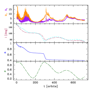
Figure 10: Retrograde high eccentricity run, tilting of the BHB - The $"{\tt retro^{**}{\color[rgb]{0,0.6,0}\mathfrak{e}}=0.9}"$ run; from the top to the bottom, panels show the individual accretion rates $\dot{M}_{1}$, $\dot{M}_{2}$ ($\times 1000$), the total inclination ${\color[rgb]{0.68,0,0}\mathrm{i}}$ in degrees, the inclination ${\rm i_{2.5}}$ towards only the inner rings, semi-major axis ${\color[rgb]{0,0,1}\mathfrak{a}}$ and the eccentricity ${\color[rgb]{0,0.6,0}\mathfrak{e}}$. See text for more details; quantities are in code units.

5.1 Physical reasons for the tilting

The retrograde setup differs in several physical properties from the prograde, such that the BHB grazes the disc without the “stream bending” within the cavity. The appearance of minidiscs is suppressed in the retrograde case, because firstly the cavity is too small to accommodate the discs and secondly because the gas inflows onto the BHs is much more radial than in the prograde case. So the gas is accreted mostly in the wake of the BHs in the retrograde case. Every direct BHB-disc interaction is thus much stronger than in the prograde case, but takes place in more closely confined space. As $\mathfrak{e}$  increases (and with it $L_{\rm Disc}/L_{\rm BHB}$) this induces an increasingly large relative movement between the CoM of the BHB with respect to the global CoM. It should be mentioned that the retrograde disc remains circular even if the BHB has high ${\color[rgb]{0,0.6,0}\mathfrak{e}}\sim 0.8$ (cf. Fig. 11, top panel). Thus, it can be understood that the BHB, which has increasingly small angular momentum, has less and less rotational support feeling the impacts into its disc more strongly with increasing ${\color[rgb]{0,0.6,0}\mathfrak{e}}$. The details for a BHB to become secularly unstable to this tilting instability will strongly be disc–model dependent, which is why we only list under which conditions we expect a system to go unstable:

1. a retrograde disc of ${\color[rgb]{0.68,0,0}\mathrm{i}}=180$°  is an unstable equilibrium configuration if $L_{\rm Disc}>2L_{\rm BHB}$ as is the case here: with growing ${\color[rgb]{0,0.6,0}\mathfrak{e}}$ the BHB is increasingly interacting with the retrograde disc, it is not off-hand to expect perturbations that are not perfectly in–plane;

2. the corotating case is stable attractor, there should be a threshold value of perturbation that leads the BHB to leave the retro-configuration in favor of the prograde one;

3. if the accretion disc is not perfectly cylindrically symmetric, but rather clumpy and of non-zero vertical extent, perturbations out-of-plane and out-of-synchronization are well possible.

It is thus not surprising that simulations where discs are light and self-gravity is not considered (e.g, Nixon, 2012; Nixon et al., 2013) would not find such an instability.

5.2 The stages of tilting

We now further explore the tilting itself, assuming that it is a physical effect. The time evolution of this run covers almost $3000$ orbits (when taking into account the very significant shrinkage of $\mathfrak{a}$(t)). After an initial increase of ${\color[rgb]{0,0.6,0}\mathfrak{e}}$ there follows circularisation which again is followed by an increase in ${\color[rgb]{0,0.6,0}\mathfrak{e}}$. At the same time the inclination $\mathrm{i}$  is decreasing then saturating and oscillating until it finally decreases. $\mathfrak{a}$  experiences several phases of strong shrinkage, whereas the accretion rate onto the primary exceeds that onto the secondary until very late times. This behavior of exchanging inclination and eccentricity is somewhat reminiscent of the Kozai–effect. However, it is not straightforward to apply these few body calculations for the BHB-disc scenario studied here: a gaseous disc is not a rigid body and can dissipate angular momentum; nor is the disc a well located point mass with clearly defined eccentricity and inclination in itself.

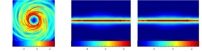
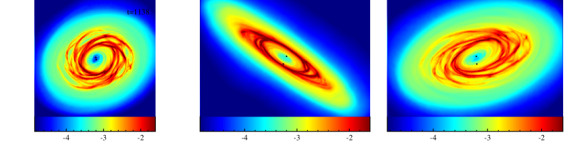
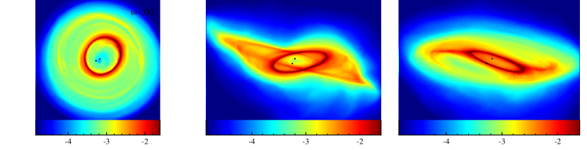
Figure 11: The tilting instability: logarithmic column density, face–on $xy$, edge–on $xz$, edge–on $yz$ - Time evolution (top to bottom) of the high accuracy, tilting $"{\tt retro^{**}{\color[rgb]{0,0.6,0}\mathfrak{e}}=0.9}"$ run. Panels show the successive stages of the binary first tilting out of plane and then subsequently aligning with the disc. Note the spread into various annuli that the disc undergoes in the middle panels.

The stages that the BHB undergoes on its way towards alignment can be subdivided into the following which are supported by Fig. 10 and 11:

1. Fast circularisation: the BHB tilts out of plane, ${\color[rgb]{0,0.6,0}\mathfrak{e}}$ quickly shrinks to ${\color[rgb]{0,0.6,0}\mathfrak{e}}\sim 0.2$, while at the same time $\mathfrak{a}$  shrinks almost by a factor of two.

2. Disc fallback I: while the BHB has shrunk very fast and circularized and tilted out of plane, the disc had disintegrated into many annuli of various inclinations due to conservation of angular momentum. Now, however, the inner part of the gas forms a flat inner disc again. Meanwhile, the gravity torques from the precessing gaseous annuli cause the BHB eccentricity to grow. It should be noted, that the CoM of the BHB and the (inner) disc have drifted apart significantly by now. The accretion rates are low and the semi-major axis remains almost stationary.

3. Inner asymmetric ring collapse: once the gas has reformed into one (inner) planar disc, the new disc-configuration has lost the formerly large BHB upkeeping the cavity size. So, at this point, it re-adjusts to the new BHB “size” and a hot, dense ring forms (cf. third panel Fig. 11). This ring has very low Toomre parameter, becomes extremely clumpy and the CoM of BHB and disc-ring drift even further apart. Note, that the cooling in the ring depends on the local orbital timescale. The fallback of gas is accompanied by large accretion rates and thus induced semi-major axis shrinkage. The BHB eccentricity remains very high.

4. Circularisation II: when finally the ring was able to cool enough for its inner part to reach the BHB, the BHB starts circularizing and tilting into the disc. The resulting meta-stable configuration has an inclination of about ${\color[rgb]{0.68,0,0}\mathrm{i}}\sim 90$° , is mildly eccentric, a stable semi-major axis and comparatively low accretion rates.

5. Disc fallback II: the initial disc has left behind some outer annuli that now start interacting with the outer part of the (inner) disc. The inner disc and the outer ring are now aligning which is accompanied by a series of precessions of the outer ring. Meanwhile the BHB increases its ${\color[rgb]{0,0.6,0}\mathfrak{e}}$ and stays in the same orientation while the disc tilts towards the BHB.

6. Outer ring collapse: Similar to stage (3), now the outer ring becomes unstable under its own gravity as it has lost too much rotational energy by aligning with the inner disc. (Most of) the outer ring collapses onto the inner disc. The accretion rates are high, but ${\color[rgb]{0,0,1}\mathfrak{a}}$ only mildly shrinks.

7. CoM alignment: Once the inner disc and the BHB are the only two major pieces reformed and the inclination is below $60$°, the BHB and its new, much more compact disc start aligning their CoMs. This is accompanied by a circularisation of the BHB, as during the interaction the BHB pushes the disc towards one side by impacting into it.

8. Standard ${\color[rgb]{0,0.6,0}\mathfrak{e}}$-growth: when finally the BHB and the disc have re-united their CoMs (apart from a tenuous outer ring), the excitation of ${\color[rgb]{0,0.6,0}\mathfrak{e}}$ similar to what was described in Roedig et al. (2011) starts occurring, while the inclination furthermore decreases.

At the final state of the simulation, the BHB has an inclination of ${\color[rgb]{0.68,0,0}\mathrm{i}}\sim 30$° , an eccentricity of about ${\color[rgb]{0,0.6,0}\mathfrak{e}}\sim 0.3$ and the secondary accretion rate is exceeding the primary. During this evolution, the drift of the total angular momentum vector was about $0.8$°, and the $\beta-$cooling has induced a loss of $L$ of about $1.2\%$. However, we do not trust the evolution past orbit $600$, because there appears noise in both the total energy and the total angular momentum and the ratio between $r_{\rm sink}$ and $\mathfrak{a}$  are severely weakening the ${\it inwards}$ torque, thus vitiating the secular effects drastically. However, from a physical point of view, the aligned, prograde state should be energetically preferred and once the disc has aligned with the BHB, it will be forced to expand its cavity analogously to the prograde case. The numerical problem of performing several thousands of orbits is challenging and we argue here that studying the entire final alignment up to ${\color[rgb]{0,0.6,0}\mathfrak{e}}\sim 0.6$ (cf. Roedig et al. (2011)) would be a waste of CPU time, since the physical arguments are quite strong if indeed the instability occurs in the first place. Also, it is our suspicion that different choices for $\beta$, cooling prescriptions, and global disc thermodynamics will alter the 8 stages identified here. The cooling, i.e. the loss of angular momentum seems to be the most crucial numerical parameter in setting the timescales for the “ring collapse” and the dissipation of the several annuli.

6 Summary

We presented numerical work on the evolution of the orbital elements of a comparable mass black hole binary surrounded by a retrograde selfgravitating disc. First, it was found that for quasi-circular BHB-disc configurations, the difference between the retrograde and prograde scenario is chiefly in the eccentricity and mass ratio evolution. The eccentricity remains close to zero in the retrograde case whereas it grows in the prograde case. The semi-major axis shrinkage was found to be the same for the circular BHB irrespective of disc (anti)alignment. For increasingly eccentric set-ups, the growth of ${\color[rgb]{0,0.6,0}\mathfrak{e}}$ was found to be exponential in time and the coupled evolution of the semi–major axis $\dot{{\color[rgb]{0,0,1}\mathfrak{a}}}$ was observed to be proportional to $\mathfrak{e}$(t), thus making the decay very efficient. Additionally, it was found that the individual accretion rates onto the two BHs grow, but that their ratio secondary over primary ${{\color[rgb]{0.25,0.1,1}\dot{M}_{2}}}/{{\color[rgb]{1,.5,0}\dot{M}_{1}}}$ assumes a maximum at eccentricities around ${\color[rgb]{0,0.6,0}\mathfrak{e}}\sim 0.45$.

We demonstrated that all the observed features can be satisfactorily explained using a simple ’dust’ model in which the BHB-disc interaction is purely gravitational. In the retrograde case, the absence of resonances together with the high BH-disc relative velocity (i.e., a small cross section) imply that the gas interacts with the binary only via direct impact onto the secondary. This is confirmed by the fact, that the turnover of ${{\color[rgb]{0.25,0.1,1}\dot{M}_{2}}}/{{\color[rgb]{1,.5,0}\dot{M}_{1}}}({\color[rgb]{0,0.6,0}\mathfrak{e}})$ could be explained by Bondi-Hoyle like accretion assuming ballistic speeds of disc-edge and binary at apocenter. Generalizing the model of N11, we find that this simple ’impact model’ is able to catch of the relevant features of the binary evolution at different eccentricities. In the prograde case, the evolution is determined by the gas inflows flung back to the disc. Treating the gas as a dust particle, we found that a simple model based on three body scattering theory fully accounts for the BHB-disc interplay. In those models, however, the mass accretion rate and instreaming rate stem from the hydrodynamical properties of the gas flow and are input parameters.

The retrograde setup shows non-negligible relative motion between the BHB center of mass and the global center of mass (CoM), even in circular runs. In the prograde case, this had been a very small effect only. There are indications that the BHB eccentricity will not grow to ${\color[rgb]{0,0.6,0}\mathfrak{e}}\sim 1$ in the retrograde case, but that the impacts into the disc inner edge destabilize the BHB until it starts moving out of the binary-disc plane. The most important physical conditions for this instability to occur be that the angular momentum of the disc exceed twice that of the BHB and that the disc be sufficiently non–axisymmetric for out-of-plane perturbations to occur. The details of the subsequent alignment are likely to be sensitive to the cooling prescription of the disc, but it is to be expected that the disc disintegrates into several annuli of various inclinations which precess within each other. It was observed that precession of the disintegrated disc annuli causes the BHB eccentricity to grow while the BHB CoM and the disc CoM do not overlap. There were stages wherein the multiple annuli aligned again to try form a coherent, flat disc. Due to loss of rotational support from the shrunk BHB, this was preceded by a short period of fragmentation-like behavior where the disc collapsed shortly into a dense ring, to spread out into spiral arms later. The BHB eccentricity exhibited few oscillations and it is expected that the final state will be a perfectly aligned disc-BHB system of eccentricity around ${\color[rgb]{0,0.6,0}\mathfrak{e}}\sim 0.6$.

We note, that it is well conceivable that, depending on the physical separation and mass, during any point of the highly eccentric phases the BHB might enter the relativistic regime and rapidly lose energy via gravitational radiation. At this point the circularization effect of gravitational radiation would compete with the eccentricity growth enforced by the retrograde disc, possibly causing a distinctive eccentricity evolution of the system that would be possibly detectable and discernible by low–frequency gravitational wave interferometers (Amaro-Seoane et al., 2013; Consortium, 2013), offering an interesting observational test of the BHB-counterrotating disc coupling.

7 Acknowledgments

CR is indebted to Kareem Sorathia and Sarah Buchanan without whom this paper would not have been written. CR is grateful to Julian Krolik and Massimo Dotti for helpful suggestions and was happy to have informative conversations with Cole Miller, Sanchayeeta Borthakur and Jens Chluba. All computations were performed on the datura cluster of the AEI and CR thanks Nico Budewitz for his HPC support. This work was funded in part by the International Max–Planck Research School, NSF grants AST-0908336, AST-1028111 and the SFB Transregio 7.

References

- Amaro-Seoane et al. (2013) Amaro-Seoane P., et al., 2013, GW Notes, Vol. 6, p. 4-110, 6, 4
- Armitage & Natarajan (2002) Armitage P. J., Natarajan P., 2002, Astrophys. J. Lett., 567, L9
- Armitage & Natarajan (2005) Armitage P. J., Natarajan P., 2005, Astrophysical Journal, 634, 921
- Artymowicz & Lubow (1994) Artymowicz P., Lubow S. H., 1994, Astrophys. J., 421, 651
- Artymowicz & Lubow (1996) Artymowicz P., Lubow S. H., 1996, Astrophys. J. Letters, 467, 77
- Bate et al. (1995) Bate M. R., Bonnell I. A., Price N. M., 1995, Mon. Not. Roy. Astr. Soc., 277, 362
- Begelman et al. (1980) Begelman M. C., Blandford R. D., Rees M. J., 1980, Nature, 287, 307
- Consortium (2013) Consortium T. e., 2013, ArXiv e-prints
- Cuadra et al. (2009) Cuadra J., Armitage P. J., Alexander R. D., Begelman M. C., 2009, Mon. Not. Roy. Astr. Soc., 393, 1423
- Cuadra et al. (2006) Cuadra J., Nayakshin S., Springel V., Di Matteo T., 2006, Mon. Not. R. Astron. Soc., 366, 358
- Gammie (2001) Gammie C. F., 2001, Astrophys. J., 553, 174
- Goldreich & Tremaine (1980) Goldreich P., Tremaine S., 1980, Astrophysical Journal, 241, 425
- Gould & Rix (2000) Gould A., Rix H., 2000, Astrophysical Journal, Letters, 532, L29
- Haiman et al. (2009) Haiman Z., Kocsis B., Menou K., 2009, Astrophysical Journal, 700, 1952
- Hayasaki (2009) Hayasaki K., 2009, Publications of the Astronomical Society of Japan, 61, 65
- Hayasaki et al. (2008) Hayasaki K., Mineshige S., Ho L. C., 2008, Astrophys. J., 682, 1134
- Hayasaki et al. (2007) Hayasaki K., Mineshige S., Sudou H., 2007, Publications of the Astronomical Society of Japan, 59, 427
- Ivanov et al. (1999) Ivanov P. B., Papaloizou J. C. B., Polnarev A. G., 1999, Mon. Not. R. Astron. Soc., 307, 79
- King et al. (2005) King A. R., Lubow S. H., Ogilvie G. I., Pringle J. E., 2005, Mon. Not. Roy. Astr. Soc., 363, 49
- Kocsis et al. (2012) Kocsis B., Haiman Z., Loeb A., 2012, Mon. Not. Roy. Astr. Soc., 427, 2660
- Kozai (1962) Kozai Y., 1962, Astronomical Journal, 67, 591
- Lin & Papaloizou (2011) Lin M.-K., Papaloizou J., 2011, ArXiv e-prints
- Lodato et al. (2009) Lodato G., Nayakshin S., King A. R., Pringle J. E., 2009, Mon. Not. R. Astron. Soc., 398, 1392
- MacFadyen & Milosavljević (2008) MacFadyen A. I., Milosavljević M., 2008, Astrophys. J., 672, 83
- Murray & Dermott (1999) Murray C. D., Dermott S. F., 1999, Solar system dynamics
- Nixon et al. (2013) Nixon C., King A., Price D., 2013, ArXiv e-prints
- Nixon (2012) Nixon C. J., 2012, Mon. Not. Roy. Astr. Soc., 423, 2597
- Nixon et al. (2011) Nixon C. J., Cossins P. J., King A. R., Pringle J. E., 2011, Mon. Not. R. Astron. Soc., 412, 1591
- Price (2007) Price D. J., 2007, Publ. Astron. Soc. Aust., 24, 159
- Quinlan (1996) Quinlan G. D., 1996, New Astron., 1, 35
- Rice et al. (2005) Rice W. K. M., Lodato G., Armitage P. J., 2005, Mon. Not. R. Astron. Soc, 364, L56
- Roedig et al. (2011) Roedig C., Dotti M., Sesana A., Cuadra J., Colpi M., 2011, Mon. Not. R. Astron. Soc, 415, 3033
- Roedig et al. (2012) Roedig C., Sesana A., Dotti M., Cuadra J., Amaro-Seoane P., Haardt F., 2012, Astronomy and Astrophysics, 545, A127
- Sesana et al. (2006) Sesana A., Haardt F., Madau P., 2006, Astrophysical Journal, 651, 392
- Shi et al. (2011) Shi J.-M., Krolik J. H., Lubow S. H., Hawley J. F., 2011, ArXiv e-prints
- Springel (2005) Springel V., 2005, Mon. Not. Roy. Astr. Soc., 364, 1105
- Springel et al. (2005) Springel V., Di Matteo T., Hernquist L., 2005, Mon. Not. Roy. Astr. Soc., 361, 776
- Syer & Clarke (1995) Syer D., Clarke C. J., 1995, Mon. Not. Roy. Astr. Soc., 277, 758
- Takeda et al. (2008) Takeda G., Kita R., Rasio F. A., 2008, Proceedings of the International Astronomical Union, 4, 181
- Volonteri et al. (2007) Volonteri M., Sikora M., Lasota J.-P., 2007, Astrophysical Journal, 667, 704