Kinetic simulation of the O-X conversion process in dense magnetized plasmas

Abstract

The ordinary-extraordinary-Bernstein (O-X-B) double conversion is considered and the O-X conversion simulated with a kinetic particle model for parameters of the TJ-II stellarator. This simulation has been done with the particle-in-cell code, XOOPIC (X11-based object-oriented particle-in-cell). XOOPIC is able to model the non-monotonic density and magnetic profile of TJ-II. The first step of conversion, O-X conversion, is observed clearly. By applying some optimizations, such as increasing the grid resolution and number of computational particles in the region of the X-B conversion, the simulation of the second step is also possible. By considering the electric and magnetic components of launched and reflected waves, the O-mode wave and the X-mode wave can be easily detected. Via considering the power of the launched O-mode wave and the converted X-mode wave, the efficiency of O-X conversion for the best theoretical launch angle is obtained, which is in good agreement with previous computed efficiencies via full-wave simulations. For the optimum angle of $47^{\circ}$ between the wave-vector of the incident O-mode wave and the external magnetic field, the conversion efficiency is $66\%$.

I Introduction

I.1 Motivation

For ensuring energy security and reduction of environmental problems, it is necessary for the world to move toward a mix of power sources such as fossil fuels, nuclear fission, fusion, and renewables. Presently, fossil fuels are the primary power source, with acute problems in environmental pollution and declining natural resources. Nuclear fission poses problems of nuclear waste, proliferation, accidental radiation release in coolant system breaches, and potentially catastrophic loss of coolant accidents such as Fukishima and Chernobyl. The renewable energy sources are dependent upon environmental conditions such as sunlight, wind, or water flow, and therefore are not continuous nor scalable. Fusion would be a source without the supply and environmental problems of fossil fuels, the waste, proliferation, and safety problems of fission, and the inability to supply consistent base load power of renwables. In the near future, fusion can provide a virtually inexhaustible source of energy energy security ; Fukishima and Chernobyl ; Environmental problems .

Energy producing fusion reactions require substantial heating and confinement. So far, the tokamak is the most promising magnetic confinement device to approach conditions necessary for net energy production. Heating the core of tokamak plasmas remains one of the key challenges in achieving fusion temperatures. One method of heating is to excite plasma waves by launching electromagnetic waves through the edge plasma into core. Dissipation of the kinetic energy of the plasma wave motion via collisions can result in heating of the plasma. Radio frequency heating is typically in three frequency ranges: the electron gyro frequency, the lower hybrid frequency, and the ion gyro frequency. The launched electromagnetic wave propagates into the plasma until it reaches a location where the magnetic field strength and the plasma density are such that one of the plasma resonance frequencies equals the wave frequency, at which point the energy of the external wave is transferred totally or partially to the plasma to excite waves in the plasma. Finally, the energy of the plasma waves is dissipated by collisions among the particles, thereby heating the plasma. A special kind of electron cyclotron (EC) wave, the electron Bernstein wave (EBW), is useful for heating the plasma core since it can penetrate beyond the cutoffs. The processes of EBW excitation have been used and simulated. Here we simulate one of these processes using the particle in cell model.

I.2 Electron Bernstein Waves

The electron Bernstein wave (EBW) is a special electrostatic cyclotron wave which propagates with a short wavelength in a magnetized hot plasma Laqua Review . After improving microwave sources to powers higher than $100\,\textrm{kW}$ and frequencies in the range of $\sim 100\,\textrm{GHz}$, and the possibility of providing over-dense plasmas in devices like Spherical Tokamaks (STs) and Stellarators, the practical use of EBW, now some years after theoretical discussions, is possible.

Due to the wave cut-off surfaces in the plasma, the electromagnetic electron cyclotron waves, e.g. the Ordinary (O) and Extraordinary (X) modes, cannot propagate in over-dense regions, so the EBW is used for heating, driving current and doing temperature diagnostics beyond these surfaces. The wavelength of the EBW is comparable with the electron gyro radius (Larmor radius). To obtain the dispersion relation, we must take into account the effects of the finite Larmor radius on the propagating wave. The Larmor radius is strongly dependent on the thermal velocity and magnetic field, so we should include the temperature of plasma species and the effect of magnetic field on the direction of wave propagation in the calculation of the dielectric tensor. In this case, we use the hot dielectric tensor Stix Book . In this level of approximation, in addition to the O-mode and X-mode electromagnetic waves obtained in the cold approximation, we have a mode named the Bernstein wave Bernstein Waves . The longitudinal electrostatic EBW is perpendicular to the external magnetic field so the generated electric field is also perpendicular to the magnetic field, i.e. $\mathbf{k}\parallel\mathbf{E}\perp\mathbf{B_{\mathbf{0}}}$.

First, it is useful to review the O and X-mode waves. These waves propagate perpendicular to the magnetic field, with cut-off and resonance points. Here, subscripts $c$ and $p$ are used for cyclotron and plasma frequencies, respectively, and $e$ and $i$ are used for electron and ion species, respectively. The dispersion relation of the O-mode wave is Miyamoto book

$$\omega^{2}=\omega_{pe}^{2}+c^{2}k_{\perp}^{2}$$ (1)

where $c$ and $k_{\perp}$ respectively are light speed and wavenumber perpendicular to the external magnetic field. It is clear from (1) that when $\omega=\omega_{pe}$ we have $k_{\perp}\rightarrow 0$ and propagation is cut-off, so the O-mode wave cannot propagate for $\omega<\omega_{pe}$. The dispersion curve of the O-mode wave is shown in Figure 1a by the blue solid line. This wave also is known as an electron plasma or Langmuir wave. The electric field component of this wave is parallel to the external magnetic field, $\mathbf{E}\parallel\mathbf{B}_{0}$.

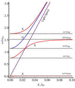
(a)

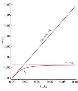
(b)

Figure 1: (a)The dispersion curve of O-mode and X-mode waves. (b) The detailed shape of lower branch of the X-mode wave.

The dispersion relation of the X-mode wave is Miyamoto book

$$\omega^{2}=\frac{(\omega^{2}-\omega_{LH}^{2})(\omega^{2}-\omega_{UH}^{2})}{(\omega^{2}-\omega_{L}^{2})(\omega^{2}-\omega_{R}^{2})}\,c^{2}k_{\perp}^{2}$$ (2)

where $\omega_{LH}$, $\omega_{UH}$, $\omega_{L}$ and $\omega_{R}$ respectively are the lower hybrid, upper hybrid, left and right-hand polarization frequencies, and are defined as Miyamoto book

$$\frac{1}{\omega_{LH}^{2}}=\frac{1}{\omega_{ci}^{2}+\omega_{pi}^{2}}+\frac{1}{\mid\omega_{ci}\omega_{ce}\mid},$$

$$\omega_{UH}^{2}=\omega_{pe}^{2}+\omega_{ce}^{2},$$

$$\omega_{L}=-\frac{\omega_{ce}}{2}+\left[\left(\frac{\omega_{ce}}{2}\right)^{2}+\omega_{pe}^{2}+\mid\omega_{ci}\omega_{ce}\mid\right]^{1/2}>0,\mbox{ and}$$

$$\omega_{R}=\frac{\omega_{ce}}{2}+\left[\left(\frac{\omega_{ce}}{2}\right)^{2}+\omega_{pe}^{2}+\mid\omega_{ci}\omega_{ce}\mid\right]^{1/2}>0.$$

As shown in Figure 1a by red solid lines, the X-mode wave has three branches. Based on their phase velocities in comparison with light speed (straight dashed line), the top and bottom branches are named respectively the fast and slow X waves, and the middle wave for $k_{\perp}\rightarrow 0$ is a fast X wave and for $k_{\perp}\rightarrow\infty$ is a slow X wave. The exact shape of the bottom branch of the X-mode wave is shown in 1b. It is clear from (2) when $\omega=\omega_{LH}$ or $\omega=\omega_{UH}$ we have $k_{\perp}\rightarrow\infty$, and consequently, resonance at these points. Conversely, when $\omega=\omega_{L}$ or $\omega=\omega_{R}$ we have $k_{\perp}\rightarrow 0$, and consequently, cut-off at these points. The region between $\omega_{LH}$ and $\omega_{L}$ and the region between $\omega_{UH}$ and $\omega_{R}$, shown in Figure 1a, are the cut-off regions for which X-mode wave propagation is forbidden. The electric field component of the X-mode wave is perpendicular to the external magnetic field, $\mathbf{E}\perp\mathbf{B}_{0}$.

The dispersion of the EBW obtained for a hot plasma approximation is Laqua Review

$$\omega^{2}=2\omega_{pe}^{2}\frac{e^{-\mu}}{\mu}\underset{n=1}{\overset{\infty}{\sum}}\frac{n^{2}I_{n}(\mu)}{1-n^{2}\omega_{ce}^{2}/\omega^{2}}$$ (3)

where $\mu=\frac{1}{2}k_{\perp}^{2}r_{L,e}^{2}$ is the finite Larmor parameter where $r_{L,e}^{2}=v_{th,e}^{2}/\omega_{ce}^{2}$ is the electron Larmor radius with $v_{th,e}$ as the electron thermal velocity. $I_{n}$ is the $n$th order modified Bessel function. Near the cyclotron harmonic resonances, the dispersion relation of the EBW has an imaginary part causing damping. So in the vicinity of the cyclotron harmonics ($\omega=n\omega_{ce}$ for integer $n$), the refractive index tends to infinity, and as shown in Figure 2, the waves are strongly absorbed in these regions Crawford dispersion curve . On the other hand, as also shown in Figure 2, there is no cut-off for EBWs due to limitation of density, and even if $\omega_{pe}/\omega_{ce}\rightarrow\infty$, the EBW would propagate in plasma. Therefore the EBWs can penetrate into the over-dense regions of plasma and cause local plasma heating and current drive.

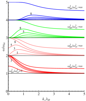
Figure 2: The dispersion curve of the EBW

If we study plasma in a full wave model (vs WKB model), can see that the middle branch slow X-mode wave has a longitudinal component that becomes dominant when the wave reaches the Upper Hybrid Resonance (UHR) point. At the UHR, the wavelength of this X-mode wave is decreasing into the range of the Larmor radius and is leading to excitation of the longitudinal EBW.

The EBW is generated only with collective cyclotron movements of electrons and it is not possible to produce the EBW in vacuum space. The most straightforward method to generate the EBW is using an electrostatic antenna with a size around the Larmor radius, but it is clear that using this antenna within a hot fusion plasma is not possible due to erosion of the antenna and impurity release into the plasma, so the practical way to excite the EBW is to use the X-mode wave with X-B conversion.

Based on the mechanism of transmission of the extraordinary wave to the UHR point to provide X-B conversion in spherical tokamaks, there are three practical methods:

1. Launch the middle branch slow X-mode wave from the side with a high magnetic field. The structure of tokamaks is such that the slow X-mode wave would not pass through any cut-off point before reaching the conversion point. But in STs, since the value of magnetic field in comparison with tokamaks is very low, this condition is difficult to meet. So this method is not popular in STs. On the other hand, this kind of X-mode can only excite the first harmonic of the EBW, which is in the low density region. This process is shown schematically in Figure 3. An experimental work using this method on the COMPASS-D Tokamak is HFSL .

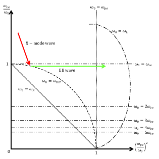
Figure 3: The schematic description of launching the slow X-mode wave from the high magnetic field side, with X-B mode conversion at the UHR.

2. Launching the top branch fast X mode from the low magnetic field side. The most important problem in this method is the existence of a cut-off layer for this branch of the X mode wave before reaching the UHR conversion point. It was proved theoretically and practically that by providing good conditions in the density gradient, it is possible for the top branch of the X-mode wave to tunnel through this layer and convert to the slow part of the middle branch, and then this wave will convert to the Bernstein wave. This process is shown schematically in Figure 4. Experiments on this mode conversion scheme have been performed at the NSTX tokamak Direct X-B .

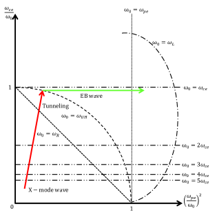
Figure 4: The schematic description of direct X-B mode conversion. In special frequencies and angles, the fast X-mode wave is able to tunnel from the right-hand cut-off and reach the UHR for X-B mode conversion.

3. Launching an O-mode wave from vacuum to produce an internal slow X-mode wave taking part in X-B conversion. This is a double O-X-B mode conversion process. The incoming O-mode wave, after reaching the cut-off point at $\omega=\omega_{pe}$, is converted to a slow X-mode wave propagating toward the UHR under special conditions. This special condition is provided if the incoming O-mode wave is cut-off at the point of the cut-off of the slow X-mode wave ($\omega=\omega_{L}$). This situation leads to coincidence of O and X waves at the same point. The conversion to the EBW mode proceeds as before, but now the higher harmonics of the cyclotron frequency are reachable. This process is shown schematically in Figure 5. The efficiency of the first O-X mode conversion is strongly depend upon the direction of propagation with respect to the external magnetic field Optimum Angle Preinhaelter ; Optimum Angle Hansen . The optimized angle between the wave-vector and the external magnetic field is

$$\theta_{opt}=\arccos\sqrt{\frac{\omega_{ce0}}{\omega_{ce0}+\omega_{pe0}}}$$ (4)

where $\omega_{ce0}$ and $\omega_{pe0}$ respectively are the cyclotron and plasma frequencies at the cut-off point of the O-mode wave. For this optimal angle, both the X and O waves are coincident at the cut-off of the O-mode wave, and have the same phase and group velocity. In this case, the power is transferred between them without any reflection. On the other hand, the transmission of energy also depends on the gradient of density, shown by the inhomogeneity scale length of density $L_{n}$. It has been shown that the best condition to have a reasonable transmission is $k_{0}L_{n}\geqslant 10$, where $k_{0}$ is the wave-number of the O-mode wave in vacuum Scale Length .

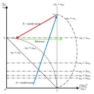
Figure 5: The schematic description of O-X-B double mode conversion. The O-mode wave reaches the cut-off point when $\omega=\omega_{pe}$, and the O-X conversion occurs under this condition for incidence angle and gradient of density: $\theta=\theta_{opt}$ and $k_{0}L_{n}\geqslant 10$.

I.3 Particle-In-Cell Model

Plasma simulation can be used to study the interaction between plasma particles and electromagnetic fields. For this purpose, two different systems are appropriate: the Vlasov–Maxwell system and the Lorentz–Maxwell system Birdsall Book . In Vlasov–Maxwell solvers, the evolution of moments of the particle distribution function is considered on a grid in phase space, and finally the required quantities are obtained via the coupling between Maxwell’s equations and the currents and charge densities given by the temporally and spatially varying distribution function. In the second method, the movement of super particles due to the Lorentz force is considered on a grid in space, and finally the required quantities are obtained via the coupling between Maxwell’s equations and the currents and charge densities obtained from particle positions and velocities. One example of a Lotentz-Maxwell system is the particle-in-cell (PIC) method.

The PIC model, due to the use of fundamental equations with only statistical approximation, often is useful for considering the nonlinear effects and the plasma collective behavior, which can be included self-consistently by coupling charged particles to the Maxwell equations via the source terms. Moreover, the study of relativistic effects via the relativistic Lorentz equation and collisional effects via Monte Carlo collisions is possible in the PIC method.

The process cycle of calculating of positions and velocities of particles each time step is shown schematically in Figure 6. First, the velocities of the particles are obtained by integration of the Lorentz equations of motion, and then the positions are obtained by integration of the respective velocities. Next, the particle losses due to absorption and gains due to emission are considered at the boundaries. In collisional models, the perturbation of velocities by elastic and inelastic collisions is considered. Then, the charge densities and currents are obtained from the positions and velocities of particles. These densities and currents are used to compute electromagnetic fields on the spatial grid by the discretized Maxwell’s equations. Finally, the Lorentz force due to these fields is used to obtain the positions and velocities of the particles in the next step time.

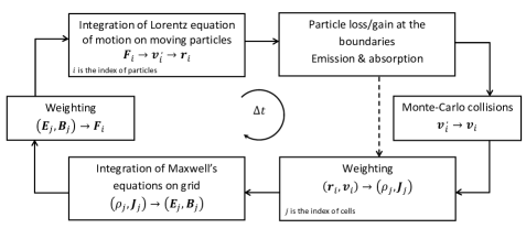
Figure 6: Calculating the positions and velocities of particles iterated in each time step

II Details of Modeling

II.1 Physical System

The most suitable device for our computational simulation is a stellarator operating in Madrid, Spain called TJ-II TJ-II-1 ; TJ-II-2 ; TJ-II-3 . This stellarator is a medium-sized flexible heliac with the following parameters: major radius $R{}_{0}=1.5\,\textrm{m}$, minor radius $a=0.2\,\textrm{m}$, and magnetic field strength on axis around $B_{0}=0.95\,\textrm{T}$. The plasma is generated and heated by launching electron cyclotron microwaves at the second harmonic, about $f=53.2\,\textrm{GHz}$. These microwaves are provided by two $300\,\textrm{kW}$ gyrotrons. Electron cyclotron resonance heating is not possible for dense regions more than $n_{e}\approx 1.7\times 10^{19}\,\textnormal{m}^{-3}$ because the second harmonic is limited by the cut-off density for this frequency. On the other hand, by providing two $800\,\textrm{kW}$ neutral beam injection systems, it is possible to heat plasma above this limit again with electron cyclotron resonance heating, but now via electron Bernstein waves TJ-II EBW . The applied scenario here is via O-X-B double mode conversion. The O-mode wave is launched from the low field side at the first harmonic $f_{0}=28\,\text{GHz}$. As shown schematically in Figure 7, the O-mode wave cannot propagate through the cutoff layer, and so is converted to the X-mode wave upon reflection. The efficiency of conversion depends on the angle of the O-mode wave with respect to the external magnetic field, and on the density gradient scale length. The optimum angle is determined via 4 and the experimental density gradient scale length is $k_{0}L_{n}\approx 30$ TJ-II kohn simulation . The converted X-mode wave propagates backward, and upon reaching the UHR layer, is converted to a quasi electrostatic Bernstein wave. This wave can penetrate deeply into high density region in the stellarator core plasma.

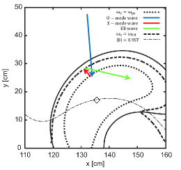
Figure 7: Poloidal cross section of TJ-II TJ-II kohn simulation .

II.2 Simulation of Physical Model

XOOPIC is a particle simulation code which has been used for modeling dense magnetized plasma. The XOOPIC (X11-based object-oriented particle-in-cell) code is an advanced two dimensional PIC code with high flexibility and extensibility due to the object oriented paradigm (OOP) XOOPIC OOP . In XOOPIC, we can simulate our system in slab or axisymmetric cylindrical geometries. The velocities and electromagnetic field vectors are considered in three dimensions, with spatial variation in two dimensions. XOOPIC includes the XGRAFIX interface that allows the user to display multiple diagnostics and view them as they evolve in time XOOPIC XGRAFIX . For obtaining the electromagnetic field, Maxwell’s equation are solved by enforcing conservation laws in discrete finite volumesXOOPIC field solvers . The density and current sources of electromagnetic field are provided by solving the relativistic equations of motion. These relativistic equations have been descretized by the relativistic time-centered Boris method PIC Review . For eliminating the problem of large angular displacements and singularity of angular momentum near the origin in axisymmetric coordinates, the position of particles is updated in a rotated Cartesian frame Birdsall Book . The incident wave is generated by a wave source implementing a surface impedance boundary condition (SIBC) XOOPIC ExitPort .

As has been shown schematically in Figure 8, we have modeled the wave conversion region using planar geometry. Its width and length respectively are $L_{x}=16\,\lambda_{0}$ and $L_{z}=42\,\lambda_{0}$ where $\lambda_{0}$ is the vacuum wavelength of the incident wave. For $f_{0}=28\,\textrm{GHz}$, $L_{x}=17\,\textrm{cm}$ and $L_{z}=45\,\textrm{cm}$. The number of cells in x and y directions are $n_{x}=4096$ and $n_{z}=1344$, respectively. Then the size of the cells is about $42\,\mu\text{m}\times 335\,\mu\text{m}$, for an aspect ratio of about $8$. The length of the input port for the incident wave is $4\,\lambda_{0}$, and comprising $128$ cells. The propagation direction of the generated electromagnetic waves for this input port in XOOPIC is perpendicular to the emitter walls XOOPIC ExitPort . In order to generate an oblique emitted wave, we divided the port into $128$ sub-ports. By adjusting the phase and amplitude of each sub-port, ultimately we established an oblique Gaussian wave propagating in the desired angle and spatial amplitude dependence. For this simulation based on 4, we have $\theta_{opt}=47^{\circ}$.

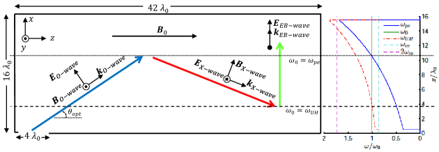
Figure 8: Schematic description of wave propagation into the plasma in the planar simulation coordinate system. Diagram of spatial dependence of plasma, cyclotron and upper hybrid frequencies in comparison with frequency of the incident wave is plotted on the right.

Since with respect to the width of the simulation region, the magnetic field variation is very small, we assumed that magnetic field is constant and according to previous simulations TJ-II kohn simulation we used $B_{0}=0.87\,\textrm{T}$. The functional behavior of density is exponential so $n(x)$ is determined as

$$n(x)=n_{0}e^{\frac{x-x_{O-cutoff}}{L_{n}}}$$ (5)

where $n_{0}$ is the density at O-mode wave cut-off position, $x_{O-cutoff}$, and $L_{n}=\left[\frac{dln\left[n(x)\right]}{dx}\right]^{-1}$ is the density inhomogeneity scale. The value of $L_{n}$, obtained from $k_{0}L_{n}=30$ TJ-II kohn simulation , is about $5.11\,\textrm{cm}$, where $k_{0}$ is the wavenumber of incident wave. The locations of the upper hybrid resonance layer and O cut-off layer, shown in Figure 8, are given by the intersection points of the upper hybrid and plasma frequencies with the constant frequency of incident wave. The values of these quantities are $x_{UHR}=3.747\,\lambda_{0}$ and $x_{O-cutoff}=10.5\,\lambda_{0}$ respectively. The diagram of the local frequencies obtained from the magnetic field and density functions and the resonance and cut off layers are shown on the right in Figure 8.

III Results

To verify the optimum angle $\theta_{opt}=47^{\circ}$, the perpendicular refractive index of O and X-mode waves along the x direction is obtained for varying parallel refractive index $N_{\parallel}=\cos\theta$. For this purpose, the wave equation

$$N\times(N\times E)+KE=0$$ (6)

is used where $N$ and $K$ are the total refractive index and the ’cold’ dielectric tensor, respectively Miyamoto book ; Laqua Review . As shown in Figure 9, by using the conditions of TJ-II, for other values of the parallel component of refractive index larger and smaller than $N_{\parallel,opt}$, the perpendicular component of refractive index $N_{\perp}$ of O or X-mode waves has an imaginary part that reduce the chance of conversion. But for $N_{\parallel,opt}=\cos\theta_{opt}=0.68$, both waves have positive $N_{\perp}^{2}$ at the conversion point, and because they coincidence at the cutoff layer, the conversion is the most probable. Thus $\theta_{opt}=47^{\circ}$ can be confirmed by PIC simulation.

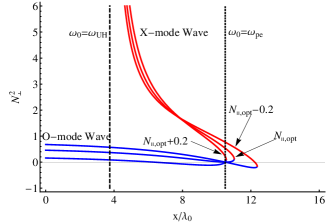
Figure 9: Perpendicular component of refractive index for a launched O-mode wave and a reflected X-mode wave in the x direction of the simulation region for TJ-II conditions for different launch angles. The O-mode coincides with the X-mode near the cutoff layer at $\omega_{0}=\omega_{pe}$. The blue and red lines are O-mode and X-mode waves, respectively.

On the other hand, it is very important to verify penetration and propagation of the EBW in the x direction and beyond the cutoff layer. For this purpose, we can use Equation 6, but now with the ’hot’ dielectric tensor Laqua Review to obtain the refractive index of the EBW. As shown in Figure 10a, for TJ-II parameters, the EBW can propagate to dense regions after passing the cutoff layer of the O-mode wave. This corresponds to the lack of density limitation shown in Figure 2. As detailed in Figure 10b, the O-X conversion happens near the O cutoff layer, and the X-B conversion occurs exactly in the UHR layer when the reflected X-mode wave reaches this layer. When $N_{\perp}$ of the X-mode wave and the EBW are equal, the X-mode wave is converted to the EBW.

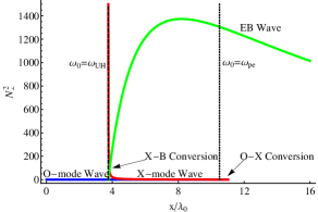
(a)

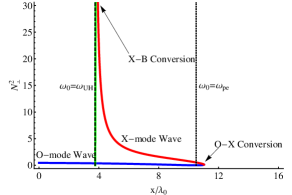
(b)

Figure 10: The mechanism of O-X-B double conversion by considering the perpendicular component of refractive index for the launched O-mode wave (blue line), reflected X-mode wave (red line) and EBW (green line) in the x direction of the simulation region for TJ-II conditions in (a) full and (b) short range. The O-X conversion occurs near the cutoff layer at $\omega_{0}=\omega_{pe}$, and X-B conversion occurs at the UHR layer at $\omega_{0}=\omega_{UH}$.

The PIC simulation was performed on a cluster of parallel computers using the MPI mechanism. The results of this simulation are divided into the following three sections:

III.1 Generation of the O-mode wave

According to Figure 8 and the value of the launch angle, we can see that the incident O-mode wave should have the $E_{x}$ and $E_{z}$ components of electric field and the $B_{y}$ component of magnetic field. As shown in Figure 11, we have adjusted the launched wave manually to be an O-mode wave. The incident wave just has $E_{x}$, $E_{z}$ and $B_{y}$ components and other components are zero, indicating the presence of the O-mode wave.

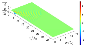
(a) $E_{x}$

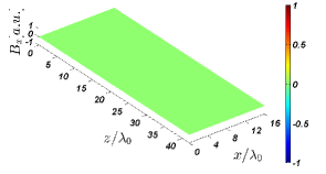
(b) $B_{x}$

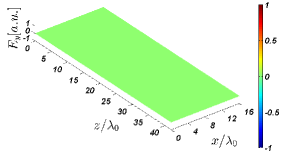
(c) $E_{y}$

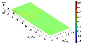
(d) $B_{y}$

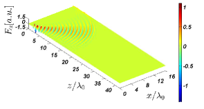
(e) $E_{z}$

(f) $B_{z}$

Figure 11: Distribution of electric and magnetic field components of the launched O-mode wave within the simulated region without plasma particles at time $t=16\,T_{wave}$, where $T_{wave}=1/f_{0}$ is time period of the launched wave.

III.2 Observation of the reflected X-mode wave

As shown in Figure 12, by considering the electric and magnetic fields of the waves, we can easily observe the O-X conversion near the O cut-off layer e.g. $x_{O-cutoff}=10.5\,\lambda_{0}$.

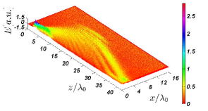
(a) $\left|\vec{E}\right|$

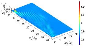
(b) $\left|\vec{B}\right|$

Figure 12: Distribution of the magnitude of (a) electric and (b) magnetic fields over the simulated region at time $t=50\,T_{wave}$, where $T_{wave}=1/f_{0}$ is the time period of the launched wave.

Based on Figure 8, the reflected X-mode wave should have the $E_{y}$ component of electric field and the $B_{x}$ and $B_{z}$ components of magnetic field. By considering Figure 13, evidence of these waves can be seen. For the reflected wave, $E_{y}$, $B_{x}$ and $B_{z}$ in comparison with other components are stronger, indicating the presence of the X-mode wave.

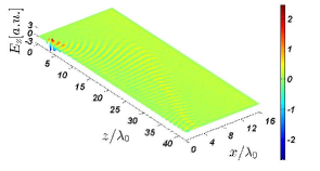
(a) $E_{x}$

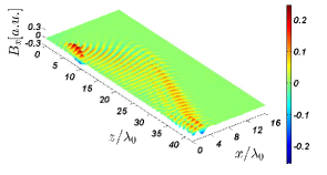
(b) $B_{x}$

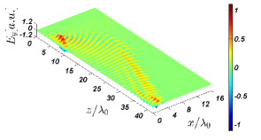
(c) $E_{y}$

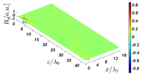
(d) $B_{y}$

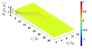
(e) $E_{z}$

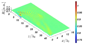
(f) $B_{z}$

Figure 13: Distribution of electric and magnetic field components over space of the simulated region at time $t=50\,T_{wave}$, where $T_{wave}=1/f_{0}$ is the time period of the launched wave.

As is evident in Figures 12 and 13, we could not observe the X-B conversion near the UHR layer, $x_{UHR}=3.747\,\lambda_{0}$. For this purpose we should increase number of grid cells and computational particles in the upper hybrid resonance layer. To achieve this, we must increase the number of computer processors to have a reasonable run time. Also we should involve thermal effects and thermal gradient in the simulation to prepare conditions for EBW propagation. In this case, then we can consider other aspects of the O-X-B double conversion. We can consider the influence of the density gradient on the conversion efficiency, and obtain the optimum gradient. Also we can consider influence of launch angle on the conversion efficiency and determine the angle for maximum net conversion, and finally we can consider parametric instability in the X-B conversion parametric instability and specify the power threshold of the instability.

III.3 O-X conversion efficiency

For considering the dependence of O-X conversion efficiency on density inhomogeneity and the angle of the launched wave, first we calculate this efficiency. We use the ratio of power propagating in the O-mode wave to the conversion region to the power transported by the X-mode wave out of this region. As shown in Figure 14, we can observe the process of O-X conversion by following the path of power propagation. Power flow near the UHR layer will ensure inclusion of incoming and outgoing power to the conversion region in our computations.

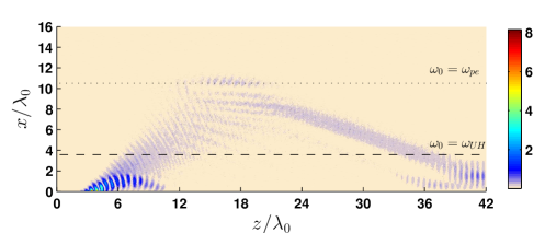
Figure 14: Distribution of electromagnetic power over the simulated region in arbitrary units at time $t=50\,T_{wave}$, where $T_{wave}=1/f_{0}$ is the time period of the launched wave. The UHR and cutoff layers are indicated by dashed and dotted lines, respectively.

The power of the electromagnetic fields along the UHR line is shown in Figure 15. Because of noisy nature of PIC simulation, this diagram exhibits a high fluctuation level, so as shown in Figure 15a, we fit the noisy diagram with a smoothing spline function by applying the De Boor approach Smoothing spline ; De Boor approach . For the noisy power $P(z_{i})$, the smoothed power $\tilde{P}(z)$ has been defined in such a way to minimize

$$\alpha\sum_{i=1}^{n_{z}}\left[\frac{P(z_{i})-\tilde{P}(z_{i})}{\delta_{i}}\right]^{2}+(1-\alpha)\intop_{0}^{L_{z}}\left[\frac{d^{2}\tilde{P}(z)}{dz^{2}}\right]^{2}dz$$

where $\alpha=0.52$ is the specified smoothing parameter and $\delta_{i}=1$ are the specified weights. The area under the curve of the incoming O-mode wave is a measure of incident power $P_{inc}$ flowing into the conversion region, and the area under the curve of the outgoing X-mode wave is a measure of converted power $P_{con}$ after mode conversion. These areas are shown in Figure 15b. With these parameters we can define conversion efficiency as $e_{con}=P_{con}/P_{inc}$. The parameters of this simulation are the same as used in the full wave model of TJ-II kohn simulation , and the obtained efficiency $e_{con}=0.66$ for $4\,\lambda_{0}$ opening width and $\theta_{opt}=47^{\circ}$, agrees well with this case in Table 1 in TJ-II kohn simulation .

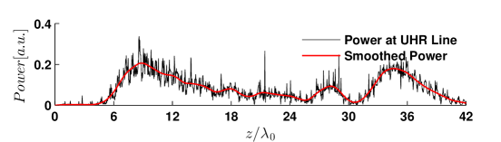
(a)

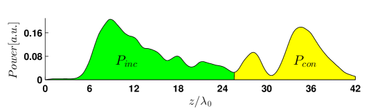
(b)

Figure 15: (a) The noisy and smoothed power along the UHR line at time $t=50\,T_{wave}$, where $T_{wave}=1/f_{0}$ is the time period of the launched wave. (b) Based on Figure 14, the regions related to the launched O-mode wave and reflected X-mode wave are determined for the smoothed power and filled up with green and yellow color, respectively. The area under the curves is a measure of incident and converted power.

IV Summary and Conclusion

A kinetic particle model for O-X conversion in a dense magnetized plasma is developed, and applied to O-mode launched at angle $\theta_{opt}=47^{\circ}$ for TJ-II parameters. The results, in good agreement with a full wave model, obtained 66% for conversion efficiency. The advantage of the kinetic model in comparison with other models like the full wave model is the ability to simulate the processes including collisional and cyclotron damping which have important effects on X-B conversion and EBW propagation. These dampings have a major impact on X-B conversion because the X-mode wave during a collisional damping converts to EBW and EBW after propagation in high density regions during a cyclotron damping transfers wave energy to plasma and leads to plasma heating full wave model .

For future work, we can consider the effects of the power of the launched wave on conversion efficiency, and also on instabilities such as the parametric instability. Effects of the density and external magnetic field profiles on conversion and instabilities will also be studied. Access to higher performance computing power will also make it possible to resolve the X-wave to EBW conversion process, which requires resolution of the EBW wavelength of the order of the electron gyro radius and sufficient computer particle density to resolve a longitudinal wave.

References

- (1) G. Bahgat, Energy Security: An Interdisciplinary Approach (West Sussex: John Wiley & Sons, 2011).
- (2) J. J. G. Cadenas, The Nuclear Environmentalist (Valencia: Springer, 2012).
- (3) F. Harris, Global Environmental Issues (West Sussex: John Wiley & Sons, 2012).
- (4) H. P. Laqua, Plasma Phys. Controlled Fusion 49, R1 (2007).
- (5) T. H. Stix, Waves in Plasmas (New York: American Institute of Physics, 1992).
- (6) I. B. Bernstein, Phys. Rev. 109, 10 (1958).
- (7) K. Miyamoto, Plasma Physics and Controlled Nuclear Fusion (Tokyo: Springer, 2004).
- (8) F. W. Crawford and J. A. Tataronis, J. Appl. Phys. 36, 2930 (1965).
- (9) V. Shevchenko,Y. Baranov, M. O’Brien, and A. Saveliev, Phys. Rev. Lett. 89, 265005-1 (2002).
- (10) G. Taylor, P. C. Efthimion, B. Jones, B. P. LeBlanc, J. R. Wilson et al., 2003 Phys. Plasmas 10, 1395 (2003).
- (11) J. Preinhaelter, and V. Kopecký, J. Plasma Phys. 10, 1 (1973).
- (12) F. R. Hansen, J. P. Lynov, and P. Michelsen, Plasma Phys. Control. Fusion 27, 1077 (1985).
- (13) F. R. Hansen, J. P. Lynov, C. Maroli, and V. Petrillo, J. Plasma Phys. 39, 319 (1988).
- (14) C. K. Birdsall and A. B. Langdon, Plasma Physics via Computer Simulation (New York: McGraw-Hill, 1991).
- (15) C. Alejaldre et al., Fusion Technol. 17, 131 (1990).
- (16) C. Alejaldre et al., Plasma Phys. Controlled Fusion 41, A539 (1999).
- (17) C. Alejaldre et al., Plasma Phys. Controlled Fusion 41, B109 (1999).
- (18) F. Castejón et al., Fusion Sci. Technol. 46, 327 (2004).
- (19) A. Köhn et al., Plasma Phys. Control. Fusion 50, 085018 (2008).
- (20) J. P. Verboncoeur, A. B. Langdon, and N. T. Gladd, Comput. Phys. Commun. 87, 199 (1995).
- (21) V. Vahedi and J. P. Verboncoeur, Proceeding of the 14th International Conference on Numerical Simulation of Plasmas (Annapolis, Maryland, 1991).
- (22) A. B. Langdon, Proceeding of the 14th International Conference on Numerical Simulation of Plasmas (Annapolis, Maryland, 1991).
- (23) J. P. Verboncoeur, Plasma Phys. Control. Fusion 47, A231 (2005).
- (24) J. H. Beggs and K. S. Yee, IEEE Trans. Antennas Propag. 40, 49 (1992).
- (25) E. Z. Gusakov and A. V. Surkov, Plasma Phys. Control. Fusion 49, 631 (2007).
- (26) C. H. Reinsch, Numer. Math. 10, 177 (1967).
- (27) C. De Boor, A Practical Guide to Splines (New York: Springer-Verlag, 2001).
- (28) A. Köhn et al., Phys. Plasmas 18, 082501 (2011).