An analytical prediction of the bifurcation scheme of a clarinet-like instrument: Effects of resonator losses

Abstract

The understanding of the relationship between excitation parameters and oscillation regimes is a classical topic concerning bowed string instruments. The paper aims to study the case of reed woodwinds and attempts to find consequences on the ease of playing.

In the minimum model of clarinet-like instruments, three parameters are considered: i) the mouth pressure, ii) the reed opening at rest, iii) the length of the resonator  assumed to be cylindrical. Recently a supplementary parameter was added: the loss parameter of the resonator (using the “Raman model”, that considers resonator losses to be independent of frequency). This allowed explaining the extinction of sound when the mouth pressure becomes very large. The present paper presents an extension of the paper by Dalmont et al (JASA, 2005), searching for a diagram of oscillation regimes with respect to the reed opening and the loss parameter. An alternative method is used, which allows easier generalization and simplifies the calculation. The emphasis is done on the emergence bifurcation: for very strong losses, it can be inverse, similarly to the extinction one for weak losses. The main part of the calculations are analytical, giving clear dependence of the parameters. An attempt to deduce musical consequences for the player is given.

Keywords : Bifurcations, Reed musical instruments, Clarinet, Acoustics.

1 Introduction

The understanding of the relationship between excitation parameters and oscillation regimes is a classical topic concerning bowed string instruments: for instance Shelleng [1], or Guettler [2], or Demoucron et al [3] proposed 2D diagrams with respect to either bow force and bow position, or bow position and bow velocity. For reed instruments, this kind of diagrams are less numerous: in Ref. [4], Dalmont et al proposed a diagram with respect to excitation pressure and reed opening, and recently Almeida et al [5] proposed a diagram with respect to blowing pressure and lip force, related to the reed opening.

In the minimum model of reed, clarinet-like instruments, three parameters are considered: i) the mouth pressure, ii) the reed opening at rest, iii) the length of the resonator  assumed to be cylindrical. In Ref. [4], a supplementary parameter was added: the loss parameter of the resonator (using the “Raman model”, that considers resonator losses independent of frequency). This allowed explaining the extinction of sound when the mouth pressure becomes very large. We notice that the agreement of the theoretical results  with experimental results was satisfactory (see Ref.  [6]).

The objective of the present paper is to revisit the paper by Dalmont et al[4]: the focus is the search for a diagram of oscillation regimes of reed instruments with respect to two parameters: the reed opening, and the loss parameter. The choice of these two parameters is justified by the fact that the third parameter, the blowing pressure, is the easiest to modify for the instrumentalist. The elements of this diagram were rather complete in Ref. [4], but phenomena occurring for strong losses, especially at the emergence of the sound, were not investigated.

The use of simplified models for the prediction of the oscillation regimes is classical for musical instruments producing self-sustained oscillations. For the calculation of the instability thresholds, linearization was used (see Wilson and Beavers [7] or Silva et al [8]), while for ab initio computation, the iterated map scheme was studied (see Mc Intyre et al [9], Maganza et al [10], Taillard et al [11]). The interest of the model chosen in the present paper is that analytical formulas are possible, given clear dependence of the parameters (for other models, numerical calculations could be possible by using similar basic ideas, using for instance continuation methods[12] or time-domain methods [13, 14]).

The analytical calculations presented hereafter are slightly different from those of Ref. [4]. They also are limited to the limit cycles corresponding to the two-state oscillating regime, but are based upon a generalization of the fact that for this regime, when no losses are present, the flow rate is a constant. This regime is the most similar to what musicians consider as a “normal” sound. In particular the method allows studying the character of the emergence and extinction bifurcations of this regime, which are important properties related to the possibility to play pianissimo or not, and more generally to the ease of playing. In Ref. [4] it was shown that the extinction bifurcation can be direct or inverse (supercritical and subcritical, respectively, see Refs; [15, 16, 17]); here it is shown that this is true also for the emergence bifurcation.

In section 2, the basic model of Ref. [4] is reminded (see also [18]), and a treatment of the problem based upon a unique quantity, the pressure difference $\Delta p,$ is presented in section 3. This leads to a simple graphical analysis of the two-state regime, explained in section 4, yielding a proof that it cannot exist with reverse flow, and an easy calculation method. Then some blowing pressure thresholds (stability, existence, …) are calculated with respect to the parameters of interest (loss, reed opening).

In section 5 the thresholds related to the instability of the regimes are calculated. Then by making two thresholds equal, the mouth pressure can be eliminated and limits of existence and stability of the static and two-state regimes are found in Section 6: this allows drawing the diagram sought. Finally a discussion is proposed concerning the existence of oscillating regimes (Section 7), with an attempt to consider more realistic models and a discussion about musical consequences.

2 The model and its parameters

We briefly remind the basic elements of the model, the non-linear characteristic of the exciter, and the origin of the iteration method, thanks to a simplified treatment of the resonator.

2.1
Nonlinear characteristics of the entering flow

In a quasi static regime, the flow $U$ entering the resonant cavity is modeled with the help of an approximation of the Bernoulli equation, as discussed e.g. in [19]. Comparison with experiment can be found in Ref. [20]. We note $P_{int}$ the acoustic pressure inside the mouthpiece, assumed to be equal to the one at the output of the reed channel, $P_{m}$ the pressure inside the mouth of the player. For small values of the difference:

$$\Delta P=P_{m}-P_{int}\text{ ,}$$ (1)

the reed remains close to its equilibrium position, and the flow $U$ is proportional to $sign(\Delta P)\sqrt{\left|\Delta P\right|}$; for larger values of this difference, the reed moves and, when the difference reaches the closure pressure $P_{c}$, it completely blocks the flow (the reed is beating). These two effects are included by assuming that if $\Delta P\leq P_{c}$ the flow $U$ is proportional to $sign(\Delta P)\sqrt{\left|\Delta P\right|}\left[P_{c}-\Delta P\right]$, and if $\Delta P>P_{c}$, the flow vanishes. Introducing the dimensionless quantities:

$$\begin{array}[]{l}p=P_{int}/P_{c}\text{ \ \ ; \ }u=UZ_{c}/P_{c}\\ \gamma=P_{m}/P_{c}\text{ ; \ }\gamma_{c}=P_{c}/P_{c}=1\text{.}\end{array}$$ (2)

where $Z_{c}=\rho c/S$ is the characteristic acoustic impedance of the cylindrical resonator, having the cross section $S$ ($\rho$ is the density of air, $c$ the velocity of sound), we obtain:

$$u=\zeta f(\Delta p)\text{ }$$ (3)

with

$$\Delta p = \Delta P/P_{c}=\gamma-p\text{ ;}$$ (4)

$$f(\Delta p) = 0\text{ \ \ if \ \ \ \ \ }\Delta p>1\text{\ ;}$$ (5)

$$f(\Delta p) = sign(\Delta p)\;(1-\Delta p)\sqrt{\left|\Delta p\right|}\text{ \ \ if }\Delta p<1\text{.}$$ (6)

The parameter $\zeta$ characterizes the intensity of the flow and is defined as:

$$\zeta=\frac{cS_{op}}{S}\sqrt{\frac{2\rho}{P_{c}}}\text{ ,}$$ (7)

where $S_{op}$ is the opening cross section of the reed channel at rest. $\zeta$ is inversely proportional to square root of the reed stiffness, contained in $P_{c}$. In real clarinet-like instruments, typical values of the parameters are $\gamma\in\left[0,1.5\right]$; $\zeta\in\left[0.1,0.5\right]$ ; values $\zeta>1$ will not be considered here, since they correspond to multi-valued functions to be solved (see Ref. [11]), and this case does not seem very realistic in practice for clarinet-like instruments. The function $f(\Delta p)$ is obviously non-analytic; it is made of three separate analytic pieces, with a singular point at $\Delta p=0$, and its derivative is discontinuous at $\Delta p=1$.

2.2 Resonator model

The resonator of length $\ell$ is assumed to be cylindrical, with zero terminal impedance. Using the d’Alembert decomposition, a change in variables at the entry of the resonator can be chosen as:

$$p(t)=p^{+}(t)+p^{-}(t)\text{ \ ; }u(t)=p^{+}(t)-p^{-}(t)$$ (8)

with the following relationship between incoming wave $p^{-}(t)$ and outcoming wave $p^{+}(t)$:

$$p^{-}(t)=-\lambda p^{+}(t-2\ell/c)$$ (9)

where $\lambda$ is the loss parameter, assumed to be independent of frequency. This is a strong assumption, necessary to obtain square signals: for certain initial conditions, all quantities remain constant in the time interval $2nl/c<t<2(n+1)l/c$. The approximation is rough for certain characteristics of the signal, such as the spectrum, but it is useful for the study of the existence, stability and amplitude of the produced sound. With this assumption, the resonator is characterized by a unique (recurrence) relation:

$$p_{n}^{-}=-\lambda p_{n-1}^{+}$$ (10)

where $2\ell/c$ is the time unit. As discussed further in section 4.2.5, losses can occur either at the extremity (radiation) or during propagation (e.g. in the boundary layers): in the latter case, if $\alpha$ is the attenuation constant per unit length, $\lambda=\exp(-2\alpha\ell),$ and the dimensionless input impedance at zero frequency is

$$\mu\overset{def}{=}\tanh(\alpha\ell)=\frac{1-\lambda}{1+\lambda}\text{ ,}\text{ \ or }\lambda=\frac{1-\mu}{1+\mu}$$ (11)

while the input impedance at the operating frequency is $1/\mu$. In what follows, the losses are characterized by the parameter $\mu$, varying between $0$ (no losses)   and $1$ (very strong losses, no wave reflection). This parameter, the reed opening $\zeta$ and the mouth pressure $\gamma$ are the three parameters of the problem. Several combination parameters will be useful:

$$\beta\overset{def}{=}\zeta\mu;\text{ \ }\beta_{1}\overset{def}{=}\zeta^{-1}\mu\text{ \ or }\zeta^{2}=\beta/\beta_{1}\text{ \ ; }\mu^{2}=\beta\beta_{1}\text{ .}$$ (12)

$\beta$ is proportional to the input impedance at zero frequency, while $\beta_{1}$ is proportional to the input admittance at the operating frequency. Two pairs of parameters can be used: either $(\zeta,\mu)$ or $(\beta,\beta_{1}).$ Notice that because $\zeta$ and $\mu$ are smaller than unity, $\beta<1$ and $\beta<\beta_{1}$, and $\beta\beta_{1}=\mu^{2}<1$. Other parameters will be useful:

$$\beta_{2}\overset{def}{=}\frac{2\beta_{1}}{1+\beta\beta_{1}}=\frac{\tanh 2\alpha\ell}{\zeta}\text{ \ ; }\beta_{3}\overset{def}{=}\frac{1}{2\beta}-\frac{3\beta_{1}}{2}.$$ (13)

3 Equations for transients and limit cycles

3.1 Recurrence for the pressure difference

Using Eqs. (3), (8) and (11), the recurrence relation (10) can be rewritten with respect to the quantities $\Delta p_{n}\overset{def}{=}\gamma-p_{n}$ and $u_{n}$. The result is:

$$2\gamma=(1+\mu)(\Delta p_{n}+u_{n})+(1-\mu)(\Delta p_{n-1}-u_{n-1}).$$ (14)

Because the flow rate $u=\zeta f(\Delta p)$ is a function of the pressure difference $\Delta p,$ this relation is a recurrence for the quantity $\Delta p$, equivalent to the recurrence used in Ref. [11] for the quantity $p^{+}$:

$$\Delta p_{n} = H^{-1}\left[K(\Delta p_{n-1})\right]\text{ \ \ with}$$ (15)

$$H(x) = x+\zeta f(x)\text{;\ \ }$$

$$K(x) = \gamma(1+\lambda)-\lambda(x-\zeta f(x)).$$ (16)

The inverse of function $H$ can be found in Ref. [11] (Appendix A).

3.2
Basic equations for the static regime

Eq. (14) is interesting in particular for the calculation of the limit cycles. For the static regime, $\Delta p$ is a constant, then

$$\gamma=\Delta p+\beta f(\Delta p)\overset{def}{=}h(\Delta p).$$ (17)

It is possible to calculate $\Delta p$ from the value of $\gamma$, or vice-versa. Concerning the stability, if the iteration function is denoted $g(x)=H^{-1}\left[K(x)\right],$ the classical stability condition is $\left|g^{\prime}(\Delta p)\right|<1$. Because $K(x)=H\left[g(x)\right],$ $dK/dx=(dH/dg)(dg/dx)$, and the condition can be written as:

$$\left[\lambda\frac{1-\zeta f^{\prime}(\Delta p)}{1+\zeta f^{\prime}(\Delta p)}\right]^{2} < 1\text{ \ }$$ (18)

$$\text{\ or \ }\left[f^{\prime}(\Delta p)+\beta_{1}\right]\left[1+\beta f^{\prime}(\Delta p)\right] > 0\text{\ }$$ (19)

(see Eq. (12)).

3.3 Basic equations for the two-state regime

For the two-state regime, because $\Delta p_{n+1}=\Delta p_{n-1}$, the following expression is found by eliminating $\gamma$ from the equation (14) written for the pairs ($n+1$, $n$) and ($n$, $n-1$):

$$h_{1}(\Delta p_{n}) = h_{1}(\Delta p_{n-1})\text{ \ \ with}$$ (21)

$$h_{1}(X)\overset{def}{=}\beta_{1}X+f(X).$$

An important property of the two-state regime is the square shape of the signal, which can be decomposed into the sum of a mean value $p_{mean}$ (zero frequency component) and an acoustic component $p_{ac}$ (sum of the odd harmonics of the operating frequency), with zero mean value:

$$p_{n} = p_{mean}+p_{ac}\text{ with }p_{mean}=\frac{1}{2}(p_{n}+p_{n-1})\text{ }$$ (22)

$$\text{and }p_{ac,n}=\frac{1}{2}(p_{n}-p_{n-1}).$$

Notice that $p_{ac,n}=-p_{ac,n-1}$, and that a similar equation can be written for the flow rate. Eq. (21) generalizes the result obtained when losses are ignored ($\mu=0)$, i.e. the constant flow rate, and it is nothing else than the input impedance relation for the acoustic component:

$$\mu(p_{n}-p_{n-1})=u_{n}-u_{n-1}.$$ (23)

It is possible to calculate the values of the two states without knowledge of $\gamma$, starting e.g. with the value of $\Delta p_{n}$: $\Delta p_{n\pm 1}$ and $\gamma$ are successively deduced from Eqs. (21) and Eq. (14). Adding the two equations (14) for the pairs ($n+1$, $n$) and ($n$, $n-1$), it is obtained:

$$\gamma_{ij} = \frac{1}{2}\left[h(\Delta p_{i})+h(\Delta p_{j})\right]\text{, or}$$ (24)

$$\gamma_{ij} = \frac{1}{2}(\Delta p_{i}+\Delta p_{j})(1-\beta\beta_{1})+\beta h_{1}\text{, }$$ (25)

with $h_{1}=h_{1}(\Delta p_{i})=h_{1}(\Delta p_{j})$ and $i=n$, and $j=n\pm 1$. Similarly for regimes with more than two states, it could be possible to start the calculation from a given state, and to deduce the other states, the prior knowledge of $\gamma$ being unnecessary. Eq. (24) is the input impedance relation for the mean value component: $p_{n}+p_{n-1}=\mu(u_{n}+u_{n-1}).$

For the two-state regime, the stability condition is $\left|g^{\prime}(\Delta p_{i})g^{\prime}(\Delta p_{j})\right|<1$, and after some algebra, the result of Ref. [4] is found (see Eq. (13)):

$$C < \beta_{2}\text{ or \ }C>\text{ }\frac{1}{\zeta^{2}\beta_{2}},\text{ }$$ (26)

$$\text{with }C = -\frac{f^{\prime}(\Delta p_{i})+f^{\prime}(\Delta p_{j})}{1+\zeta^{2}f^{\prime}(\Delta p_{i})f^{\prime}(\Delta p_{j})}.$$ (27)

4 Existence of the static and two-state regimes

The previous results can be applied whatever the shape of the function $f(\Delta p).$ The present section investigates the existence of the static and two-state regimes for the particular shape of the function given by Eqs. (5) and (6).

4.1 Static regime

For negative $\Delta p$, the function $f(\Delta p)$ is negative too, therefore the static regime does not exist for negative flow (and positive excitation pressure $\gamma$). For $\Delta p>1$, the static regime exists for $\gamma=\Delta p>\gamma_{c}=1$. The pressure $p=\gamma-\Delta p$ vanishes: this is obvious because the reed closes the input of the resonator.

Otherwise, for a non-beating reed, the study of the function in the right-hand side of Eq. (17) shows that it increases from $0$ to $1$ when $\Delta p$ increases from $0$ to $1.$ Therefore a unique solution exists  for $0<\gamma<1$.

4.2 Two-state regime

4.2.1 Number of solutions

For the two-state regime, two values of $\Delta p$, with the same value of the function $h_{1}(X)$ are sought. They do not depend on the impedance at zero frequency, i.e. on the value of $\beta.$ The study of $h_{1}(X)$ leads to the following results (see Fig. 1): for negative $X$, the derivative $h_{1}^{\prime}(X)$ is always positive, while for positive $X$, it is positive up to $X=\Delta_{M}$, where $\sqrt{X}$ is the positive root of the following equation:

$$3X-2\beta_{1}\sqrt{X}-1=0,\text{ \ i.e.}$$ (28)

$$X=\Delta_{M}\text{ \ with \ }\Delta_{M}=\frac{1}{9}\left[\beta_{1}+\sqrt{\beta_{1}^{2}+3}\right]^{2}.$$ (29)

For $X>1$ (beating reed), the value of the derivative is $\beta_{1}$, and is positive. Two cases need to be distinguished: if $\Delta_{M}>1$, i.e. if $\beta_{1}>1$, the derivative is always positive and it is impossible to find two values of $X$ with the same value $h_{1}(X).$ On the contrary, for

$$\beta_{1}<1,$$ (30)

the function decreases from $h_{1}(\Delta_{M})$ to $\beta_{1}$ when $X$ increases from $\Delta_{M}$ to $1$, then re-increases. Solutions of Eq. (21) can be found in this case only, and the corresponding value of the function is necessarily larger than $\beta_{1}$. A consequence is that Eq. (21) has no solution for $h_{1}(X)<\beta_{1}$, and this is true in particular for negative $h_{1}(X)$. Therefore no two-state regime can be found with negative flow. This conclusion is compatible with the general result obtained for all possible regimes in Ref. [11]. Because of this result, the paper is now focused on positive pressure differences $\Delta p.$

For $h_{1}(X)\in\left[\beta_{1},h_{1}(\Delta_{M})\right]$, three values of $X$, defined as $X_{a}<X_{b}<X_{c}$ lead to the same value of the function (see Fig. 1), and three two-state regimes are possible, which can be either non-beating (for the pair ($X_{a}$, $X_{b}$)) or beating (for the pairs ($X_{a}$, $X_{c}$) and ($X_{b}$, $X_{c}$)). The intervals of the three solutions are as follows: $X_{a}\in\left[\beta_{1}^{2},\Delta_{M}\right]$ ; $X_{b}\in\left[\Delta_{M},1\right]$ ; $X_{c}\geq 1$.

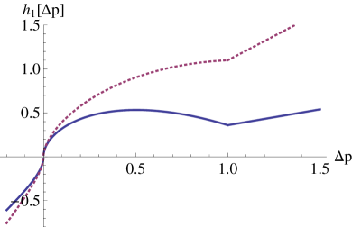
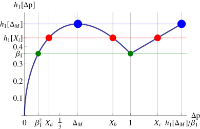
Figure 1: Left: Function $h_{1}(\Delta p)$ for two values of $\beta_{1}$. Dotted line: $\beta_{1}=1.1$ (monotonous variation). Solid line: $\beta_{1}=0.36$. Right: Zoom for the second case. A maximum value exists at $P_{M}=(\Delta_{M},$ $\ h(\Delta_{M})).$ The middle horizontal line corresponds to $h_{1}(X)=0.452$, with the 3 solutions $X_{a}$, $X_{b}$, $X_{c}.\$The two other horizontal lines exhibit the limits of existence of the two-state regime.

From the solution of Eq. (21), the corresponding excitation pressure $\gamma$ for the two-state regime is given by Eq. (24), for the three pairs of solutions $(\Delta p_{i},\Delta p_{j})=(X_{i},X_{j})$. For the particular case of the beating-reed regime, when $h_{1}=\beta_{1}\Delta p_{c}$, and  $i=a,b,$ the expression can be also written as:

$$\gamma_{ic} = \frac{1}{2}\left[h(\Delta p_{i})+\frac{h_{1}(\Delta p_{i})}{\beta_{1}}\right]$$ (31)

$$= \Delta p_{i}+\frac{f(\Delta p_{i})}{\beta_{2}}\overset{def}{=}h_{2}(\Delta p_{i})\text{ }.\text{ }$$ (32)

4.2.2 Existence, beating, saturation and extinction thresholds

• At the limit of existence, when $h_{1}^{\prime}(\Delta p)$ vanishes,

  $$\Delta p_{a}=\Delta p_{b}=\Delta_{M}.$$ (33)

  Therefore the existence threshold $\gamma_{th}$ of the two-state regime is:

  $$\gamma_{th}=\Delta_{M}+\beta f(\Delta_{M})=h(\Delta_{M})$$ (34)

  The solutions can be either stable or unstable, i.e. the bifurcation can be direct or inverse. This is discussed hereafter in section 5.2.2.

• Another limit of existence is given by $X_{b}=1.$ Using, Eq. (31), this yields: $\gamma=\gamma_{c}=1.$ The solutions can be either stable or unstable, i.e. the bifurcation can be direct or inverse. This is discussed hereafter in section 5.2.1.

• The beating threshold $\gamma_{b}$ appears when one solution is $X=1,$ $h_{1}(X)=\beta_{1}$, thus the pair of solution is: $X_{a}=\beta_{1}^{2},$ $X_{b}=1;$ therefore, using Eq. (31):

  $$\gamma_{b}=h_{2}(\beta_{1}^{2}).$$ (35)

  Because $\beta_{1}^{2}<1$, and $0<\beta<\beta_{1}$, the threshold $\gamma_{b}$ can be shown to be always smaller than the closure threshold $\gamma_{c}=1$.

• The saturation threshold is obtained for the beating regime, with $dp_{a}/d\gamma=0,$ with $p_{a}=\gamma-X_{a}$, i.e. $dX_{a}/d\gamma=1$, therefore $X_{a}=1/3$, $\gamma_{sat}=h_{2}(1/3),$ and

  $$\text{ \ }p_{a}=\frac{2}{3\sqrt{3}\beta_{2}};\text{ }u=f\left(\frac{1}{3}\right)\text{ =}\frac{2\zeta}{3\sqrt{3}}=u_{\max}$$ (36)

  At the saturation value, the flow rate is maximum: $u=u_{\max}$. For $\beta_{1}>1/\sqrt{3},$ the saturation threshold is the beating threshold, because for $\beta_{1}^{2}=1/3$, $\gamma_{sat}=\gamma_{b}$: the amplitude of the pressure decreases from the beating threshold.

• Finally the overcritical (extinction) threshold $\gamma_{e}$ is given by $d\gamma/d\Delta p_{i}=0$ in Eq. (31). This condition yields to the following result:

  $$3\Delta p_{a}-2\beta_{2}\sqrt{\Delta p_{a}}-1=0,\text{ or }$$ (37)

  $$\Delta p_{a} = \frac{1}{9}\left[\beta_{2}+\sqrt{\beta_{2}^{2}+3}\right]^{2}\text{ }=\Delta p_{e}\text{ }$$ (39)

  $$\text{and }\gamma_{e}\overset{def}{=}h_{2}(\Delta p_{e}).$$

  Because $\Delta p_{e}<1$, it exists if $\beta_{2}<1$ only. As explained in Ref. [4], when losses tend to $0$ ($\beta_{2}$ tends to $0$), the extinction threshold tends to infinity. The threshold $\gamma_{e}$ is always larger than $\gamma_{c}=1$, because $\sqrt{\Delta p_{e}}-\beta_{2}=(1-\Delta p_{e})/(2\sqrt{\Delta p_{e}})$, thus:

  $$\gamma_{e}-\gamma_{c}=\frac{1}{\beta_{2}}\frac{(1-\Delta p_{e})^{2}}{2\sqrt{\Delta p_{e}}}\geq 0.$$ (40)

4.2.3 Subcritical threshold at emergence (non-beating reed)

Results (34) to (39) were obtained with other, equivalent methods in Ref. [4]. However another threshold can exist for the non-beating case ($i=a$, $j=b$): for certain values of the parameters, the emergence bifurcation can be inverse, and the threshold of oscillation is different for crescendo and decrescendo playing. The subcritical threshold $\gamma_{sc}$ can be calculated by using the change in variables defined in Ref. [4]:

$$\Sigma\overset{def}{=}\sqrt{X_{a}}+\sqrt{X_{b}}\text{ ; }\Pi\overset{def}{=}\sqrt{X_{a}}\sqrt{X_{b}}.$$ (41)

Eq. (21) implies:

$$\Pi=\Sigma^{2}-\beta_{1}\Sigma-1$$ (42)

(this change in variables is related to the decomposition into dc and acoustic components, see Eq. (22)). The threshold can be calculated by writing $d\gamma/d\Sigma=0$ in Eq. (24), which can be written as a polynomial in $\Sigma$ (see Eq. (A17) in Ref. [4]). For our purpose, it is convenient to write this equation as follows (denoting $\gamma=\gamma_{ab})$:

$$\gamma=\beta(\varphi-\beta_{3})(\varphi^{2}-1)+\gamma_{b}\text{ \ with }\varphi\overset{def}{=}\Sigma-\beta_{1},$$ (43)

where $\beta_{3}$ is given by Eq. (13). Notice that $\varphi_{b}=1.$ The derivative $d\gamma/d\varphi$ vanishes for $\varphi=\varphi_{sc}$:

$$3\varphi_{sc}^{2}-2\beta_{3}\varphi_{sc}-1 = 0\text{ \ or }$$ (44)

$$2\varphi_{sc}(\varphi_{sc}-\beta_{3}) = 1-\varphi_{sc}^{2}\text{ \ \ \ or }$$ (45)

$$\varphi_{sc} = \frac{1}{3}\left[\beta_{3}+\sqrt{\beta_{3}^{2}+3}\right].$$ (46)

Therefore, $\varphi_{sc}$ is always positive, and combining Eqs. (43) and (45), it is shown that the threshold $\gamma_{sc}$ is always smaller than the beating-reed threshold:

$$\gamma_{sc}=\gamma_{b}-\frac{\beta}{2\varphi_{sc}}(1-\varphi_{sc}^{2})^{2}.$$ (47)

4.2.4 Solutions

The direct solution of the cubic equation (43) is possible (see footnote 4). In the present paper we propose a method based upon Eqs. (21) and (25). Starting from a value of $X_{a}\in\left[\beta_{1}^{2},\Delta_{M}\right]$, the solution $X_{c}$ (above unity) is obtained by $X_{c}=h(X_{a})/\beta_{1}$, and the solution $X_{b}$ is deduced by solving the equation $h_{1}(X_{b})=h_{1}(X_{a})$ for $X_{b}\in$ $\left[\Delta_{M},1\right]$. The latter equation is cubic in $\sqrt{X_{b}}$. It has a solution already known, $\sqrt{X_{a}}$, therefore $\sqrt{X_{b}}$ can be deduced as the positive solution of a quadratic equation, as follows:

$$x^{2}-(\beta_{1}-\sqrt{X_{a}})x-h_{1}(X_{a})/\sqrt{X_{a}}=0\text{, where }x=\sqrt{X_{b}}.$$

$$X_{b}=\frac{1}{4}\left[\beta_{1}-\sqrt{X_{a}}+\sqrt{(\beta_{1}+\sqrt{X_{a}})^{2}+\frac{4f(X_{a})}{\sqrt{X_{a}}}}\,\right]^{2}.$$ (48)

From the knowledge of the three solutions of $h_{1}(X)=h_{1}(X_{a})$, the three values of $\gamma_{ij}$ are deduced from Eq. (25). Figures 2 and 3 show 4 examples of bifurcation schemes for different cases. The calculation is done by varying the starting value $X_{a}$ and was verified using the iterated map algorithm (Ref. [11]), which obviously gives stable solutions only. The three straight lines $p=\gamma-\beta_{1}^{2}$, $p=\gamma-\Delta_{M}$, and $p=\gamma-1$ delimit the three domains of solutions, $X_{a}$, $X_{b}$ and $X_{c}.$ The solution is non-beating for the pair ($X_{a}$, $X_{b}$)) or beating, for the pairs ($X_{a}$, $X_{c}$) and ($X_{b}$, $X_{c}$)), see Fig. 1.

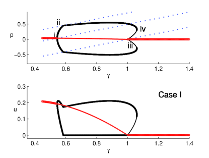
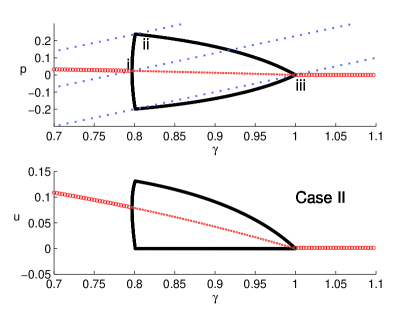
Figure 2: Two examples of bifurcation schemes for the pressure $\gamma,p$ and the flow rate $\gamma,u$. The emergence bifurcation is direct. The three dotted (blue), increasing straight lines indicate the three domains of solutions $X_{a},$ $X_{b}$, and $X_{c}$. Case I, left: $\zeta=0.55$, $\mu=0.2$.The solid curve corresponds to a two-state regime, which is stable (thick line) or unstable (thin line): the emergence bifurcation is direct, while the extinction bifurcation is inverse. The pale (red), decreasing line corresponds to the static regime, which is stable (thick line) or unstable (thin line). The point $i$ indicates the instability threshold $\gamma_{th}$ of the static regime; the point $ii$ the beating threshold $\gamma_{b}$ of the two-state regime; the point $iii$ is the closure threshold $\gamma_{c}=1$,  the point $iv$ is the extinction threshold $\gamma_{e}$ of the two-state regime. Case II, right: $\zeta=0.4$, $\mu=0.3$. Both emergence $i$ and extinction bifurcations $iii$ are direct. The point $ii$ indicates the beating threshold $\gamma_{b}$ of the two-state regime. Because $\beta_{1}=.75>1/\sqrt{3}$, saturation occurs at the beating threshold $\gamma_{b}.$

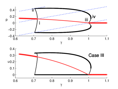
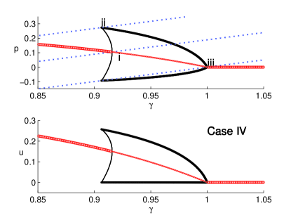
Figure 3: Two examples of bifurcation schemes for the pressure $\gamma,p$ and the flow rate $\gamma,u$. The emergence bifurcation is inverse. The three dotted (blue), increasing straight lines indicate the three domains of solutions $X_{a},$ $X_{b}$, and $X_{c}$. Case III, left: $\zeta=0.88$, $\mu=0.45$. Both emergence and extinction bifurcations are inverse. The point $iv$ indicates the overcritical (extinction) threshold $\gamma_{e}$ of the two-state regime, and the point $iii$ the closure threshold $\gamma_{c}=1$ of the static regime. Case IV, right: $\zeta=0.88$, $\mu=0.7$. The extinction bifurcation is direct.

Figure 4 shows the diagram ($\Delta p,\gamma$) for the case I of Figure 2. This allows exhibiting the function $h(\Delta p),$ given by Eq. (17), for the static regime and the function $h_{2}(\Delta p)$, given by Eq. (31), for the beating, two-state regime. The one-state regime is stable from $\{0,0\}$ to $\{\Delta_{M},\gamma_{th}\}$ and above $\{1,1\}$. The non-beating two-state is given by Eqs. (24) and (48), the beating two-state is given for $X_{a}<1$ by the function $h_{2}(X)$. The bifurcation at emergence is direct, the oscillation is stable from $\{\Delta_{M},\gamma_{th}\}$ to $\{\beta_{1}^{2},\gamma_{b}\}$. The beating two-state is stable from $\{\beta_{1}^{2},\gamma_{b}\}$ to $\{\Delta p_{e},\gamma_{e}\}$ and unstable between $\{\Delta p_{e},\gamma_{e}\}$ and $\{1,1\}$. The oscillation amplitude is at a maximum at $\{1/3,\gamma_{s}\}$, where the slope of $h_{2}(X)$ is unity.

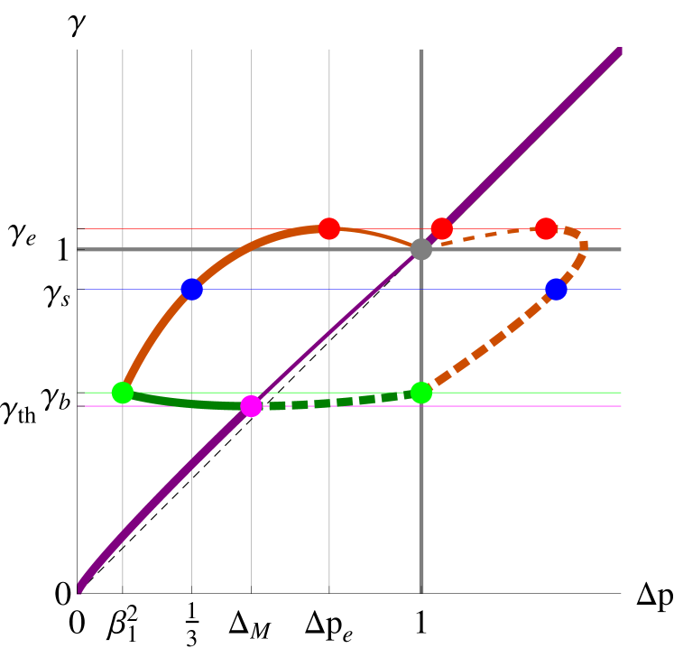
Figure 4: Representation for $\Delta p$,$\gamma)$. The function $h(\Delta p)$ is used for the static regime (black curve, purple in color) and the function $h_{2}(\Delta p)$ for the beating, two-state regime (grey curve, brown in color). The non-beating two-state (light grey, green in color) is given by Eqs. (24) and (48). Thick lines: stable regime, thin lines: unstable regime. Dashed lines: solution of the 2-state regime with the high value of $\Delta p$. The points signal the transitions at the different thresholds.

4.2.5 Radiated sound

The radiation losses are small at low frequencies, therefore it is very simple and classical to deduce them by perturbation from the output flow rate, considering a monopole radiation. Two cases have to be distinguished: losses occur at the output, or losses occur during propagation into the tube. Both cases give the same input impedance, but not the same transfer functions between input and output. The latter case is more realistic, and is considered here. If the output impedance is $0,$ and losses due to boundary layers only, the output acoustic flow rate is given by the standard transmission lines relationships: $u_{out}=\sinh(j\omega\ell/c+\alpha\ell)p_{ac}$, where $\omega\ell/c=\pi/2$ (see section 3.2). Therefore the amplitude relationship is the following:

$$\left|u_{out}\right| = \left|p_{ac}\right|/\cosh(\alpha\ell)=$$

$$\left|p_{ac}\right|\sqrt{1-\mu^{2}} = \left|u_{ac}\right|\frac{\sqrt{1-\mu^{2}}}{\mu}.$$

The maximum output acoustic flow rate is obtained for the saturation threshold; at the saturation threshold, because the reed is beating, $\left|u_{ac}\right|=(u_{\max}+0)/2=\zeta/(3\sqrt{3}),$(see Eq. (36)). For $\beta_{1}=\mu/\zeta<1/\sqrt{3},$ the saturation threshold is the beating threshold (see section 4.2.2), and $p_{ac}=(1-\beta_{1}^{2})/2$, therefore:

$$\left|u_{out}\right|_{\max} = \frac{\sqrt{1-\mu^{2}}}{3\sqrt{3}\beta_{1}}\text{ if }\beta_{1}>\frac{1}{\sqrt{3}};$$ (49)

$$\left|u_{out}\right|_{\max} = \frac{1}{2}(1-\beta_{1}^{2})\sqrt{1-\mu^{2}}\text{if }\beta_{1}<\frac{1}{\sqrt{3}}.$$

For a given value of $\zeta$, this is monotonously decreasing function of $\mu$; for a given value of $\mu$, this is a increasing function of $\zeta.$

5 Calculation of instability thresholds  

The stability conditions (18) and (26) are calculated using the expression of the derivative $f^{\prime}(\Delta p)$:

$$\text{ }f^{\prime}(\Delta p) = \frac{1-3\Delta p}{2\sqrt{\Delta p}}\text{ \ if }\Delta p<1\text{ ;}$$

$$\text{ }f^{\prime}(\Delta p) = 0\text{ if }\Delta p>1.$$ (50)

5.1 Instability of the static regime

The condition (18) generalizes the condition $f^{\prime}(\Delta p)>0$, as discussed in Ref. [21] for the lossless case (see page 349). For the (static) beating reed case, which exists for $\gamma>\gamma_{c}=1$ (see previous section), $f^{\prime}(\Delta p)=0$, thus the static regime is always stable. For the non-beating reed case, the first factor of Inequality (18) is equal to $h_{1}^{\prime}(\Delta p)$, thus it vanishes when $\Delta p$ satisfies Eq. (28), i.e. $\Delta p=\Delta_{M}$. For this value, $\Delta_{M}$, the second factor of Inequality (18) is $(1-\beta\beta_{1})$, which is positive. Thus (29) together with Eqs. (17) gives the threshold $\gamma_{th}$, given by Eq. (34).

Therefore the condition $h_{1}^{\prime}(\Delta p)=0$ gives both the limit of existence of the two-state regime (see Eq. (34)), and the instability threshold of the static regime. Nevertheless the nature (direct or inverse) of the bifurcation between the two regimes is not yet solved by this result. The term $\beta f(\Delta_{M})$ is the static pressure $p_{s}$  in the mouthpiece; the presence of the parameter $\beta$ indicates that the threshold depends on the impedance at zero frequency.

5.2 Instability of the two-state regime

5.2.1 Beating-reed case: overcritical (extinction) threshold

For the beating regime $f^{\prime}(X_{c})=0$, with $X_{i}<1,$ thus, using Condition (26), $C=-f^{\prime}(X_{i})$  for $i=a$ or $b$. Because $C<1$, and because $\zeta^{2}\beta_{2}=\zeta\tanh 2\alpha\ell<1$, the second inequality (26) is never valid. Therefore the stability is defined by the condition $C<\beta_{2}.$

When $\beta_{2}>1$, this condition is always satisfied, and the beating two-state regime is stable (no overcritical threshold $\gamma_{e}$ exists, as noticed in Section 4.2.2).

When $\beta_{2}<1$, Eq. (37) is used, yielding $\beta_{2}=(3\Delta p_{e}-1)/(2\sqrt{\Delta p_{e}})$. The function $(3x-1)/(2\sqrt{x})$ being always increasing for positive $x$, the inequality $C<\beta_{2}$ holds if $X_{i}<\Delta p_{e}$, or $p_{i}>p_{e}=\gamma-\Delta p_{e}.$ This distinguishes in the ($\gamma,p$) plane the two branches separated by the overcritical threshold: the upper one is stable, while the lower one is unstable. The unstable branch is the branch joining the static regime, because the two regimes cannot be stable for the same value of the parameter $\gamma$ when they converge to the same point. This can be explained with mathematical arguments, based upon either a perturbation method (see Ref. [15]) or the topological degree (see Ref. [16]). This can be also studied by using Inequalities (26), as done in Ref. [4].

It can be noticed that because $\gamma_{e}$ is larger than unity, the beating, two-state regime is always stable for $\gamma_{b}<\gamma<\gamma_{c}=1$, whatever the value of $\beta_{2}.$

5.2.2 Non-beating case: period doubling and subcritical (emergence) threshold

i) For the non-beating regime ($i=a$, $j=b$), an expression of the instability threshold was given in Ref. [4] and it was explained that the threshold is given by $1/C=\zeta^{2}\beta_{2}$. Some errors were done in the derivation, and they are corrected in appendix A of the present paper. When the excitation pressure is larger than this threshold, here denoted $\gamma_{ins}$, period doubling can occur, then a complex bifurcation scenario (see Ref. [11]).

ii) Otherwise, it can be checked that the second condition $C=\beta_{2}$ leads to the subcritical emergence threshold $\gamma_{sc}$: it separates two branches in the ($\gamma,p)$ plane, the upper one being stable while the lower one is unstable. This is similar to what happens for the overcritical threshold. When it exists, the emergence bifurcation is as follows: when playing crescendo, the oscillation starts for $\gamma=\gamma_{th}$, while playing decrescendo, the oscillation stops for $\gamma=\gamma_{sc}.$

When this subcritical threshold can exist? From Eq. (43) and (44), it is found that

$$\gamma_{th}-\gamma_{sc}=\beta(\varphi_{th}-\varphi_{sc})^{2}\left[\frac{1}{2\varphi_{sc}}+\frac{\varphi_{sc}}{2}+\varphi_{th}\right]$$ (51)

where $\varphi_{th}=\Sigma_{th}-\beta_{1}$ and $\varphi_{th}-\varphi_{sc}=\Sigma_{th}-\Sigma_{sc}$, with

$$\text{ }\Sigma_{th}=2\sqrt{\Delta_{M}}=\frac{2}{3}\left(\beta_{1}+\sqrt{\beta_{1}^{2}+3}\right)\text{.}$$ (52)

Two cases are possible:

• $\Sigma_{sc}>\Sigma_{th}$: the emergence bifurcation is direct: stable solutions exist for $\gamma>\gamma_{th}$.

• $\Sigma_{sc}<\Sigma_{th}$: the emergence bifurcation is inverse, and stable solutions exist for $\gamma>\gamma_{sc}.$

When $\Sigma_{sc}$ continues to decrease below $\Sigma_{th}$, the bifurcation remains inverse, but the subcritical threshold $\gamma_{sc}$ becomes the beating threshold $\gamma_{b}$. This happens when $\Sigma_{sc}=\Sigma_{b}=1+\beta_{1}$, or $\varphi_{sc}=\varphi_{b}=1$ (notice that the inequality $\Sigma_{b}\leq\Sigma_{th}$ always holds). The discussion is extended in section 6.3.

6 Limits of regimes in the plane ($\mu,\zeta)$  

From the different expressions of the thresholds, it is possible to deduce the limits separating different domains in the plane $(\mu,\zeta)$, as shown in Fig. 5. Above the diagonal (region 0), no two-state regime can exist. Other regions of the plane are defined by the nature of the emergence and extinction bifurcations: they are named by the number of the four cases shown in Figures Figures 2 and 3: in Regions I and III, the extinction bifurcation is inverse, while in Regions II and IV, it is direct. What is new in this paper is the separation between Regions I and II, with direct emergence bifurcation, and regions III and IV, with inverse emergence bifurcation. Finally, in Region V, the two-state regime can be unstable, and can be replaced by more complicated regimes, with period doubling, chaos, intermittences, etc… (see Ref. [11]).

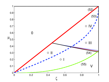
Figure 5: Plane $(\zeta,\mu).$ The four Regions I to IV correspond to the different cases presented for the examples shown in Figs. 2 and 3. The chosen values for the examples are indicated by a circle. In Region V period doubling or other regimes can exist, in Region 0 no sound is possible. The numbers refer to the equation number. Above line (53), no sound is possible. Curve (54) distinguishes the extinction bifurcation (direct above, inverse below). Curve (55) distinguishes the emergence bifurcation (direct above, inverse below). Below curve (56), complicated regimes can appear by destabilization of the two-state regime. The two curves close to the curve (55) correspond to equations (59), and (60), from to the top to the bottom (see section 6.3).

6.1 Emergence and extinction bifurcations

• When the instability threshold $\gamma_{th\text{ }}$(Eq. (34)) of the static regime reaches the closing threshold $\gamma_{c}=1$, the static regime becomes stable whatever the values of all parameters, and no sound can be expected. This happens for $\beta_{1}>1$, and this confirms the result explained in section 4.2.1 that no two-state regime can exist (this discussion is extended in the next section). The condition for the existence of sound can be also written as:

  $$\mu<\zeta\text{, or \ \ }\lambda>\frac{1-\zeta}{1+\zeta}\text{ .}$$ (53)

• When the overcritical threshold $\gamma_{e}$ (Eq. (39)) reaches the closure threshold of the static regime $\gamma_{c}=1$ (Eq. (35)), the extinction bifurcation becomes direct instead of inverse, as explained in the previous section. For $\beta_{2}<1,$ the bifurcation is inverse: this is probably the most frequent case for real clarinets and clarinettists, and corresponds to:

  $$\zeta>\tanh 2\alpha\ell=\frac{2\mu}{1+\mu^{2}},\text{ or \ \ }\lambda>\sqrt{\frac{1-\zeta}{1+\zeta}}.$$ (54)

  Between the two limits (53) and (54), the extinction bifurcation is direct (Regions I and IV).

• When the subcritical threshold $\gamma_{sc}$ (Eq. (46)) reaches the instability threshold of the static regime $\gamma_{th}$ (Eq. (34), the emergence bifurcation becomes direct. From Eq. (51), this happens when $\varphi_{sc}=\varphi_{th}$. The bifurcation is direct in Regions I and II, with the following condition:

  $$\beta<\frac{\Sigma_{th}-\beta_{1}}{\beta_{1}\Sigma_{th}+3}.$$ (55)

6.2 Limit of instability of the two-state, non-beating regime

Finally, when the instability threshold $\gamma_{ins}$ of the oscillating regime given by the condition $1/C=\zeta^{2}\beta_{2}$ (see section 5.2.2) reaches the beating threshold $\gamma_{b}$, the limit was given in Ref. [4] (with a small error). The formula can be obtained from Eq. (26), for $X_{a}=\beta_{1}^{2}$, and $X_{b}=1$, $f^{\prime}(X_{b})=-1.$ The limit $\zeta_{i}$ is given by the following equation:

$$\frac{1-f^{\prime}}{1-\zeta^{2}f^{\prime}}=\frac{1}{\zeta^{2}\beta_{2}}\text{ \ where }f^{\prime}=f^{\prime}(X_{a})=\frac{1-3\beta_{1}^{2}}{2\beta_{1}}.$$ (56)

This leads to a second order equation in $\zeta^{2}$:

$$\beta_{1}^{2}(1-3\beta_{1}^{2})\zeta^{4}+(4\beta_{1}^{2}-3\beta_{1}+1)(\beta_{1}+1)\zeta^{2}-2\beta_{1}=0.$$ (57)

A particular value is $\beta_{1}=1/3$, $f^{\prime}=1$, $\zeta_{i}=1$, $\mu=1/3$, $\lambda=1/2$. For a given loss coefficient $\mu$ $(<\zeta)$, the two-state regime is always stable when $\zeta<\zeta_{i}$. For sake of simplicity, we remark that an excellent approximation of the limit, better than 1%, is based upon the fact that for small losses, the coefficient $\beta=\zeta^{2}\beta_{1}$ is small, therefore $\beta_{2}\simeq 2\beta_{1}$:

$$\zeta_{i}^{2}\simeq\frac{1}{2\beta_{1}(1-f^{\prime})+f^{\prime}}.$$ (58)

6.3 Limits related to the beating threshold

Another limit is reached when the subcritical threshold $\gamma_{sc}$ becomes the beating-reed threshold $\gamma_{b}$, thus the stable two-state regime is always beating. However the unstable branch is non-beating (see Figs. 2 and 3). Using Eq. (47), it is found to be given by $\varphi_{sc}=\beta_{3}=1$, i.e.

$$\beta<\frac{1}{3\beta_{1}+2}\text{ \ }.$$ (59)

A last limit is reached when the instability threshold of the static regime $\gamma_{th}$ (34) reaches the beating threshold of the two-state regime $\gamma_{b}$, i.e. when $\varphi_{th}=\Sigma_{th}-\beta_{1}=\beta_{3}$ in Eq. (43):

$$\beta=\frac{1}{\beta_{1}+2\Sigma_{th}}.$$ (60)

For both limits given by Eqs. (59) and (60), the corresponding curves are therefore within Regions III and IV of Figure 5. They are very close to the limit given by Eq. (55), corresponding to the change in nature of the emergence bifurcation. The three limits are even equal for $\beta_{1}=1$, $\beta=1/5$, $\mu=\zeta=1/\sqrt{5}.$ For a given $\zeta$, when losses are small ($\mu$ small), the emergence bifurcation is direct. Then, when $\beta$ reaches the limit (55), the bifurcation becomes inverse, with a non-beating reed. Then, when $\beta$ reaches the limit given by Eq. (59), the bifurcation remains inverse, but the reed becomes always beating in the two-state regime.

Fig. 6 shows details of the bifurcation scheme ($\Delta p,\gamma)$ near the subcritical threshold for different cases between the non-beating case $\gamma_{th}<\gamma_{b}$ and the beating case $\gamma_{b}<\gamma_{th}$ (for the latter case, the beating threshold is the subcritical threshold, as for the points III and IV). The corresponding values of the parameter ($\zeta,\mu$) are extremely close together.

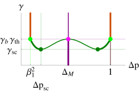
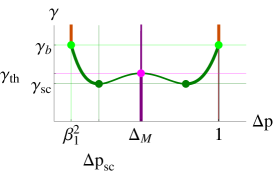
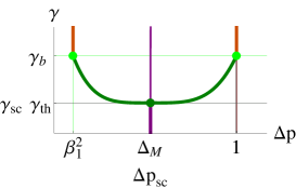
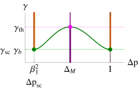
Figure 6: Zoom of bifurcation diagrams with sub-critical threshold. $\beta_{1}=0.68$ Left up: case $\gamma_{sc}=\gamma_{th}$, $\beta=0.24584;$ Right up: case $\gamma_{sc}<\gamma_{th}<\gamma_{b}$, $\beta=0.24532$; Left down: case $\gamma_{th}=\gamma_{b}$, $\beta=0.24752$ Right down: case $\gamma_{sc}=\gamma_{b}$, $\beta=0.24322.$

7 Influence of losses on the existence of the two-state regime

When losses tend to infinity ($\mu$ tends to unity), no sound is possible whatever the value of $\zeta$: this is in accordance with the intuition that if no reflection exists at the input of the resonator, no self-sustained oscillation can happen. Nevertheless, we do not prove that other types of regimes cannot exist, such as four-state, eight-state, … In this section, this issue is discussed together with the influence of the choice of the model. Moreover, some musical consequences are discussed.

7.1 Possibility of existence of other oscillating regimes

When the static regime is always stable ($\beta_{1}>1$), it has been proved that the two-state regime cannot exist. It is probable that other types of regimes do not exist, but the general proof is difficult. Using the calculation of the successive iterates functions for different values of the initial condition (see Ref. [11]), we verified that when $\beta_{1}>1$, the successive iterates converge to the unique point that is the limit cycle of the static regime, thus no other regime can exist. This can be done for every set of parameter values, $\gamma$, $\zeta$, $\mu<\zeta$: if the convergence is always to a unique state, then it is sure that no other regime than the static one can exist. Obviously, this verification is not possible in practice, but the verification has been done for some set of parameter values.

We conclude that no oscillating regime exists for $\beta_{1}>1$, even if the rigorous sentence should be: no oscillating regime exists by destabilization of the static regime. A similar discussion could be done for the destabilization of the two-state regime into more complicated regimes (see section 6.2).

7.2 Influence of the choice of the model

7.2.1 Model for the beating reed

The method used in the present paper can also be used for any shape of the nonlinear characteristic, at least numerically (the condition being that a nonlinear characteristic is static). All equations of sections 2 and 3 remain valid when modifying the nonlinear function $f(\Delta p).$ In particular if a smooth beating transition is chosen with no singularity, Fig. 1 shows that the condition (30), $\beta_{1}<1$, can be generalized into the following condition: the function $h_{1}(\Delta p)$ goes through both a maximum and a minimum.

7.2.2 Frequency dependence of losses

The Raman model is interesting because all quantities can be determined analytically, but it is not very realistic. It is based upon two important assumptions: losses do not depend on frequency, and the reed has no dynamics. A generalization of the present study is out of the scope of the present paper, but it is interesting to note that the condition $\beta_{1}<1$ can be easily generalized when these assumptions are not done, as explained hereafter.

When losses depend on frequency, it is possible to use the characteristic equation obtained by linearizing the nonlinear equation around the pressure of the static regime $p_{s}$, and writing the approximation of the first harmonic:

$$u = F(p)\simeq F(p_{s})+(p-p_{s})F^{\prime}(p_{s})$$ (61)

$$\text{ }u = Y_{1}p$$ (62)

where $Y_{1}$ is the admittance of the fundamental frequency. The characteristic equation is written as:

$$F^{\prime}(p_{s})=Y_{1}$$ (63)

As it is well known (see Ref. [22]), this gives the condition $\ Im(Y_{1})=0$, thus the playing frequency $f_{p}$ at the threshold can be deduced. Moreover, if at this frequency, $\beta_{1}\overset{def}{=}Y_{1}/\zeta$, the pressure threshold is given by:

$$f^{\prime}(\Delta p_{s})=-\beta_{1}$$ (64)

because $F(p)=\zeta f(\Delta p).$ Therefore $\Delta p_{s}$ satisfies Eq. (28):

$$\Delta p_{s}=\Delta_{M}\text{ \ and }\gamma_{th}=\Delta_{M}+p_{s}$$ (65)

as expected in section 5.1. As a consequence, when the losses depend on frequency, the value of the threshold is the same as for the Raman model, and the limit of existence of the two-state regime $\beta_{1}=1$ is unchanged. Nevertheless the hypothesis has been done that the small oscillations are sinusoidal (on this subject, see Refs. [23], [22] or [24]), and this is not true for inverse bifurcation. When several harmonics interact, the problem becomes much more intricate, especially because of resonance inharmonicity. Moreover taking into account the frequency dependence of the losses leads to a distinction between the threshold of the fundamental regime and the “overblown” regimes (see Ref. [12]): this distinction does not exist with the Raman model, which allows a distinction based upon the initial conditions only.

As a summary, it can be said that if we suppose that the impedance peak of the operating frequency is higher than the other ones, the emergence bifurcation is direct and the limit $\beta_{1}=Y_{1}/\zeta=1$ is valid. This is true in particular for the first register of a clarinet and a part of the second register. The large increase of radiation losses at higher frequency due to the open toneholes lattice (see e.g. Ref. [25]) does not affect the highest peak, therefore the main result of the present paper can be extrapolated to a large number of notes of a real clarinet.

7.2.3 Effect of the reed dynamics

When the reed dynamics is taken into account as that of a 1 dof oscillator, the following characteristic equation has been obtained by Silva et al [8]:

$$Y_{1}=\zeta\sqrt{\gamma}\left[\frac{1}{1+j\theta/Q_{r}-\theta^{2}}-\frac{1-\gamma}{2\gamma}\right]$$ (66)

where $\theta=\omega/\omega_{r}$, $\omega_{r}$ is the reed-resonance angular frequency, and $Q_{r}$ its quality factor. The threshold pressure and frequency can be deduced from this equation, and were studied in this paper; here we are interested in the limit for which the static regime becomes always stable, i.e. when $\gamma=1.$ If the input impedance of the resonator is considered around a resonance frequency $\omega_{1}$, it is possible to write:

$$Y=Y_{1}\left[1+jQ_{1}\left(\frac{\omega}{\omega_{1}}-\frac{\omega_{1}}{\omega}\right)\right]$$

where $Q_{1}$ is the quality factor of the resonance. For $\gamma=1,$ the real part of Eq. (66) leads to the following result:

$$\beta_{1}=\frac{1}{1-\theta^{2}+Q_{r}^{-2}\frac{\theta^{2}}{1-\theta^{2}}}.$$ (67)

For a lossless reed, $\beta_{1}=1/(1-\theta^{2})>1$: the limit of the losses in the tube allowed for having a sound is increased by the reed dynamics, which favors the sound production. But the effect of the reed  losses is to decrease the limit. It can be concluded that reed losses and resonator losses act in the same sense concerning the range of parameter allowing sound production (this conclusion is valid for the direct-bifurcation case).

7.3 Discussion about musical consequences for the player

The previous results can be useful in order to understand and teach important aspects of the sound control by the instrumentalist. Such an objective knowledge should largely increase the pedagogical efficiency. Otherwise the approach of the problems remains more subjective and the explanations can be lengthy and less clear. One of the most useful aspects is about pianissimo playing. The bifurcation diagrams show that the players have two possibilities: near the emergence and near the extinction. The first possibility is used for playing dolce, with a quasi monochromatic sound, but the sound is noisy and cannot be sustained for a long time, due to high value of the airflow $u$ (see Fig. 2, case I). The dynamic is not easy to control because of the steepness of the bifurcation diagram near $\gamma_{th}$. The second possibility, near $\gamma_{e}$, conducts to a clean pianissimo, with a sound richer in high harmonics. This can however only be achieved by crossing the curve (54) in Fig.5, in order to reach the region II where the extinction bifurcation is direct.
This property is usually unknown by the players (the ability of playing such a “magical” pianissimo is often attributed exclusively to the “quality” of the reed). The beginners reduce the reed opening ($\zeta)$ by “biting” the reed and this causes unwanted effects: the pitch rises considerably, due to the decrease of the effect of the reed flow rate (see [26], and such a bending stress can cause a plastic (irreversible) deformation of the reed. The skilled player can reach region II by increasing the damping due to the lip and use a high blowing pressure near the extinction threshold, playing in the reverse way (decreasing the mouth pressure for playing louder, see Fig. 2, case II). The lip comes very near to the tip of the reed, with a moderate lip pressure. This effect is probably similar to an increase of $\beta_{1}$, resulting in a displacement of the playing parameters on the $(\mu,\zeta)$ plane exactly in the wanted direction, increasing the value of $\mu$ and decreasing the value of the parameter $\zeta$ proportionally to $\sqrt{\beta_{1}}$. The decrease in $\zeta$ is probably due to an increase of the reed stiffness. Decreasing $\zeta$ without “biting” too much could also be achieved by modifying the hydrodynamics of the airflow entering the channel, in order to increase the vena contracta, but to our knowledge no experimental evidence shows that the player can indeed modify significantly the vena contracta. Conversely, it seems that the parameter $\beta$ cannot be significantly controlled by the player (in another way than by modifying the length of the air column). In real life, this parameter of static airflow resistance may not be determined only by the length and the diameter of the bore but certainly also by hydrodynamic effects near the channel, due to the viscosity of the air. This acts in a similar but possibly stronger way than the static resistance of the bore. Practical tests show that the effects predicted in the zones III and IV are indeed observed in some pathological situations, despite the fact that our theoretical model would require many meters of a tube of small diameter to obtain such high values of $\beta$.

To include the musician mouth in the model is obviously rather complicated, even if at low frequencies, the effect of the vocal tract is not important. Therefore the previous analysis requires some conjectures. Besides the problems of bifurcation, the analysis of the Raman model permits establishing some facts useful for the musician:

• The calculation of the mean flow shows that the most economical blowing pressure is near the beating threshold in Region I (corresponding to normal playing). This explains that skilled players can sustain the sound significantly longer than beginners.

• The transients are much faster if $\zeta$ is large (see Ref. [18]); weak reeds help doing this, as well as using a moderate lip pressure. This simplifies the staccato learning.

• The effects of leaks in the air column (misplacement of a finger, defective pads) increase the value of $\beta_{1}$, so that regions 0, and probably III or IV can be possibly visited (see section 7.2.2). Almost any control can be destroyed over the dynamics (or at least rendering the dynamic control more difficult), despite of the attempts of the clarinettist to supply more energy to the instrument by opening the embouchure, increasing $\zeta$.

8 Conclusion

The present paper is focused on limit cycles corresponding to two-state regimes, and is a complement to the paper [11], which was focused on transients. Thanks to a formulation focused on the pressure difference between mouth and mouthpiece, the effect of the nonlinear function on the production of the two-state regime can be analyzed, and especially the role of the losses. The map shown in Fig 5 can certainly be improved by using more complex models, but we think that some results are robust. When the reed opening at rest is very small or when the reed stiffness is very large (i.e. when the dimensionless parameter $\zeta$ is very small), losses can be too large and the sound production becomes impossible. A complement to this conclusion is the following: for $\zeta$ larger than $1/\sqrt{5}$, when losses increase, the emergence bifurcation becomes inverse before the sound disappears, and the instrument becomes more difficult to play. For $\zeta$ smaller than this value, when losses increase, there is a direct passage from the direct emergence bifurcation to the absence of sound.

9 Acknowledgements

This work was supported by the French National Agency ANR within the SDNS-AIMV and CAGIMA projects. We thank also the high school ARC-Engineering in Neuchâtel. Finally we wish to thank Philippe Guillemain and Christophe Vergez for fruitful discussions.

10 Appendix: correction to the Ref. [4]

The instability threshold $\gamma_{ins}$ of the oscillating regime is given by the condition $1/C=\zeta^{2}\beta_{2}$ (see Ineqs. (26), it is the limit of unstable solutions toward period-doubling of the two-state regime). This leads to the following equation, if $\Sigma$ and $\Pi$ are defined by Eq. (41):

$$\frac{4\Pi}{\zeta^{2}}+(1+3\Pi)^{2}-3\Sigma^{2}=\frac{4\beta_{1}}{1+\beta\beta_{1}}\Sigma(3\Pi-1)$$ (68)

Together with Eq. (42) leads to a fourth-order equation in $\Sigma$; from the solution $\Sigma$ the value the threshold of instability $\gamma_{ins}$ is deduced by using Eq. (43). Another method is to start from certain values of the parameter $\beta_{1}$ and of the solution $\Sigma$, then to deduce $\Pi$ using Eq. (42), then $\beta$, which is solution of a second order equation

In Ref. [4], Eq. (A23) was correct, but a factor 4 was missing in Eq. (A24), the correct equation being the present Eq. (68). Then Eq. (A25) needs to be corrected by introducing a factor 4 on the right-hand side, and the factor $(2+3\Pi)$ needs to be replaced by $(12\Pi-1)$ in Eq. (A28) and similarly $(2+3\Pi_{0})$ needs to be replaced by $(12\Pi_{0}-1)$ in Eq. (A30).

Concerning the limit $\gamma_{ins}=\gamma_{b}$, Eqs. (A32) to (A34) of Ref. [4] are corrected in Section 6.2 of the present paper. The last equation gives the coefficient $\beta_{1}$ as a series expansion of the limit $\zeta_{i}$:

$$\beta_{1}=\frac{\zeta^{2}}{2}\left[1-\zeta^{2}+\frac{5}{4}\zeta^{4}-\zeta^{6}\right]$$ (69)

This expression corrects Eq. (A34) of the previous paper (the correction is small, because the order 6 in $\zeta$ only is concerned), but this approximation is much less accurate than the present Eq. (58).

References

- [1] Schelleng, J.C., “The bowed string and the player,” J. Acoust. Soc. Am. 53, 1973, 26–41.
- [2] K. Guettler, K. On the creation of the Helmholtz movement in the bowed string. Acta Acustica united with Acustica 88 (2002) 970–985.
- [3] Demoucron, M., Askenfelt A. and Caussé, R., Measuring Bow Force in Bowed String Performance: Theory and Implementation of a Bow Force Sensor, Acta Acustica united with Acustica, 95, 2009, 718 – 732.
- [4] Dalmont, J.-P. , Gilbert, J., Kergomard, J. and Ollivier, S. “An analytical prediction of the oscillation and extinction thresholds of a clarinet”. J. Acoust. Soc. Am., 118, 2005, 3294–3305.
- [5] A. Almeida, J. Lemare, M. Sheahan, J. Judge, R. Auvray, Kim Son Dang, S. John, J. Geoffroy, J. Katupitiya, P. Santus, A. Skougarevsky, J. Smith and J. Wolfe , Clarinet parameter cartography: automatic mapping of the sound produced as a function of blowing pressure and reed force Proceedings of the International Symposium on Music Acoustics, 2010, Sydney, Australia.
- [6] Dalmont, J.-P. and Frappé, C.,“ Oscillation and extinction thresholds of the clarinet: Comparison of analytical results and experiments”. J. Acoust. Soc. Am., 122, 2007, 1173–1179.
- [7] Wilson, T.A. and Beavers, G.S. , “Operating modes of the clarinet”. J. Acoust. Soc. Am., 56, 1974, 653-658.
- [8] F. Silva, J. Kergomard, C. Vergez and J. Gilbert, Interaction of reed and acoustic resonator in clarinetlike systems, J. Acoust. Soc. Am. (2008) 124 3284-3295
- [9] McIntyre, M. E. , Schumacher, R. T., and Woodhouse, J. . On the oscillations of musical instruments. J. Acoust. Soc. Am., 74, 1983, 1325–1345.
- [10] Maganza, C., Caussé, R. and Laloë, F. . “Bifurcations, period doubling and chaos in clarinetlike systems”, Europhysics letters 1, 1986, 295–302.
- [11] Taillard, P.-A., Kergomard, J., and Laloë, F., Iterated maps for clarinet-like systems, Nonlinear Dynamics 62, 2010, 1-19.
- [12] Karkar, S. Vergez, C. and Cochelin, B., Oscillation threshold of a clarinet model: A numerical continuation approach, J. Acoust. Soc. Am., 131, 2012, 698-707.
- [13] Guillemain, P., Kergomard, J., Voinier, T., Real-time synthesis of clarinet-like instruments using digital impedance models, J. Acoust. Soc. Am., 118, 2005, 483-494.
- [14] Takahashi K., Kodama, H., Nakajima, A., Tachibana, T., Numerical study on multi-stable oscillations of woodwind single-reed instruments, Acta Acustica united with Acustica, 95, 2009, 1123-1139.
- [15] Iooss, G. and Joseph, D.D., Elementary stability and bifurcation theory. Undergraduate texts in Mathematics, Springer Verlag, 1980.
- [16] Sattinger, D.H., Topics in stability and bifurcation theory, Lecture notes in mathematics, Springer Verlag, 1973.
- [17] Strogatz, S.H., Nonlinear Dynamics and Chaos: with Applications in Physics, Biology, Chemistry, and Engineering, Addison-Wesley, Reading, MA, 1994.
- [18] Kergomard, J., “Elementary considerations on reed-instrument oscillations”. In Mechanics of musical instruments, vol. 335 (A. Hirschberg/ J. Kergomard/ G. Weinreich, eds),of CISM Courses and Lectures, pages 229–290. Springer-Verlag, Wien, 1995.
- [19] Hirschberg, A. , Van de Laar, R. W. A. , Marrou-Maurires, J. P. , Wijnands, A. P. J., Dane, H. J. , Kruijswijk, S. G. and Houtsma, A. J. M. “A Quasi-stationary Model of Air Flow in the Reed Channel of Single-reed Woodwind Instruments”. Acustica, 70, 1990, 146–154.
- [20] Dalmont, J.-P., Gilbert, J. and Ollivier, S. . “Nonlinear characteristics of single-reed instruments: quasistatic volume flow and reed opening measurements”, J. Acoust. Soc. Am., 114, 2003, 2253–2262.
- [21] Fletcher N. and T. Rossing, T., The physics of musical instruments, Springer Verlag, 1991.
- [22] Grand, N., Gilbert, J., Laloë, F., Oscillation threshold of woodwind instruments. Acta Acustica 1, 1997, 137-151.
- [23] Worman, W.E., Self-sustained nonlinear oscillations of medium amplitude in clarinet-like systems. PhD thesis, Case Western Reserve University, 1971.
- [24] Ricaud, B., Guillemain, P., Kergomard, J., Silva, F., Vergez, C., Behavior of reed woodwind instruments around the oscillation threshold, Acta Acustica united with Acustica, 95, 2009, 733-743.
- [25] Moers, E., Kergomard, J., On the Cutoff Frequency of Clarinet-Like Instruments. Geometrical versus Acoustical Regularity, Acta Acustica united with Acustica, 97, 2011, 984 – 996.
- [26] Dalmont, J. P. Guillemain, Taillard, P.A., Influence of the reed flow on the intonation of the clarinet. Acoustics 2012 Nantes, 2012, 1173–1177.