Possibility of direct observation of edge Majorana modes in quantum chains

Abstract

Several scenarios for realization of edge Majorana modes in quantum chain systems: spin chains, chains of Josephson junctions, and chains of coupled cavities in quantum optics, are considered. For all these systems excitations can be presented as superpositions of a spinless fermion and a hole, characteristic for Majorana fermion. We discuss the features of our exact solution with respect to possible experiments, in which edge Majorana fermions can be directly observed when studying magnetic, superconducting, and optical characteristics of such systems.

Majorana fermions (MF) are particles, identical to own antiparticles. They may appear as elementary neutral particles, or emerge as quasiparticles in many-body systems Wil . During last years MF, besides being of fundamental interest of their own, have attracted great attention as the basis for potential application in topological quantum computation Kit1 . The search for MF is among the most prominent tasks for modern physicists. During last few years a great progress has been achieved in such a search in condensed matter physics. Obviously, we cannot expect MF to exist in ordinary metals, because excitations, electrons, considered as quasiparticles there, and their counterparts, holes (which linear combination would correspond to the MF), can destruct each other: they carry opposite charges. Hence, the search in different, non-standard systems of fermions with special properties, where MF can exist as emergent non-trivial excitations, is necessary. Superconducting systems seemingly provide a basis for such states, because elementary excitations there are superpositions of electrons and holes. However, for conventional superconductors with, e.g., $s$-wave pairing, those superpositions of electrons and holes carrying opposite spin are different from Majorana’s construction. Then it follows that for a system of spinless fermions with pairing, like e.g., model superconductors with $p$-pairing in one dimensional (1d) systems Kit , or with $(p+ip)$-pairing in 2d ones KS , MF can emerge. Among the most known predicted candidates for MF existence are topological insulators FK , and semiconducting quantum wires LSS , where pairing can be achieved by interfacing them with an ordinary superconductor. The modern “state of art” of theoretical predictions for realizations of such systems has been recently reviewed, e.g., in Al . While recent papers Mour claim that they have observed zero bias anomalies in the tunneling conductance of normal conducting and superconducting systems, which can be explained by the presence of zero energy MF, very recent publications mention that in those experiments the spatial resolution could be not enough to detect MF, and that disorder can result in zero bias features Liu even for non-topological system (where MF are absent). That is why, proposals for realization of direct observations of MF are highly desirable.

In the present work we consider several scenarios for the direct observation of edge MF in quantum chains, which can be realized in quantum magnetic, superconducting, and optical systems. For all these systems excitations can be presented as superpositions of spinless fermions and holes, the hallmark of MF. We choose 1d systems, because exact theoretical results can be obtained there, which is very important for comparison with experiment, and due to the significant success in fabrication and manipulation of quasi-1d materials in recent years. We propose to use an external parameter, which directly governs the behavior of the edge MF in those quantum chains.

To set the stage, we start with the consideration of the spin-1/2 chain, which Hamiltonian is

$${\cal H}_{0}=-\sum_{n=1}^{N-1}(J_{x}S_{n}^{x}S_{n+1}^{x}+J_{y}S_{n}^{y}S_{n+1}^{y})-J_{x}^{\prime}S_{0}^{x}S_{1}^{x}-J_{y}^{\prime}S_{0}^{y}S_{1}^{y}\ .$$ (1)

Here $S_{n}^{x,y}$ are operators of the projections of spin 1/2 at the $n$-th site, $J_{x,y}$ ($J^{\prime}_{x,y}$) are coupling constants for the host (impurity situated at the site $n=0$). To realize the manifestation of edge MF in observable characteristics, we propose to study the system with the Hamiltonian ${\cal H}={\cal H}_{0}-hS_{0}^{x}$. The local field $h$, acting at the edge site of the chain, can be realized if the spin chain system neighbors a ferromagnet, which is magnetized along the $x$ axis. Let us (formally) add the spin $S_{-1}$ at the left edge of the chain with the coupling $-2hS_{0}^{x}S_{-1}^{x}$, to study the Hamiltonian ${\cal H}_{M}={\cal H}_{0}-2hS_{0}^{x}S_{-1}^{x}$ instead of ${\cal H}$ KT ; Zb . We see that ${\rm Tr}_{N+1}(\rho S_{0}^{x})={\rm Tr}_{N+2}[\rho_{M}S_{0}^{x}(1+2S_{-1}^{x})]\equiv 2{\rm Tr}_{N+2}(\rho_{M}S_{0}^{x}S_{-1}^{x})$, where $\rho$ ($\rho_{M}$) is the density matrix with the Hamiltonian ${\cal H}$ (${\cal H}_{M}$). It means that to obtain the average value of the operator of edge spin projection with ${\cal H}$, we can calculate the one for the pair correlation function with ${\cal H}_{M}$. After the Jordan-Wigner transformation with Dirac creation (destruction) fermionic operators $d^{\dagger}_{m}$ ($d_{m}$) we get

$${\cal H}_{M}=-{1\over 2}[h(d_{-1}^{\dagger}d_{0}+d_{-1}^{\dagger}d_{0}^{\dagger}+{\rm H.c.})+I^{\prime}(d_{1}^{\dagger}d_{0}+d_{0}^{\dagger}d_{1})$$

$$+J^{\prime}[d_{1}^{\dagger}d_{0}^{\dagger}+d_{0}d_{1}]+\sum_{n=1}^{N-1}(I[d_{n}^{\dagger}d_{n+1}+d_{n+1}^{\dagger}d_{n}]$$

$$+J[d_{n}^{\dagger}d_{n+1}^{\dagger}+d_{n+1}d_{n}])]\ ,$$ (2)

where $I,J=(J_{x}\pm J_{y})/2$, $I^{\prime},J^{\prime}=(J_{x}^{\prime}\pm J_{y}^{\prime})/2$. In what follows we consider the limit $N\to\infty$ (semi-infinite chain). Eq. (2) is, in fact, the Hamiltonian of the inhomogeneous Kitaev toy model Kit (the Hamiltonian of the homogeneous Kitaev toy model has the same form as the fermionic representation for the Hamiltonian of the XY spin-1/2 chain introduced in Ref. LSM, ) with $I\to w$, $w$ is the hopping parameter of spinless electrons, and $J\to|\Delta|$, $\Delta$ is the induced superconducting (sc) gap, or the $p$-wave pairing amplitude of the 1d topological superconductor FK ; Al , or a quantum wire LSS ; Al with zero chemical potential of electrons and with inhomogeneities of hopping amplitudes and gaps near the edge of the chain. Zero chemical potential in Kitaev’s model permits the topological superconductivity, i.e., the weak pairing regime, in which the size of Cooper pair is infinite (see below). The model Eq. (2) can also describe the 1d system of coupled cavities with strong in-cavity photon-photon repulsion and nonlinear photon driving BT in the cavity quantum electrodynamics. There necessary re-definitions are $J\to{\hat{\Delta}}$, where ${\hat{\Delta}}$ is the magnitude of the photon driving, and $I\to{\hat{J}}$, where ${\hat{J}}$ is the tunneling amplitude for photon hopping between nearest neighbor cavities. The term with $h$ describes the interaction of the edge cavity with the light BT . Our model is related to photons being in resonance with cavities. It has been also pointed out recently that Kitaev’s model can be realized in 1d arrays of Josephson junctions vHAHBB : the chain of sc islands coupled via strong Josephson junctions to a common ground superconductors. Each island contains a pair of MF at the endpoints of a semiconductor nanowire. The parameters of our Hamiltonian are related to the one of the inhomogeneous array of Josephson junctions as: $J^{y}\to E_{M}$, where $E_{M}$ is the tunnel coupling of individual electrons between sc islands: $J^{x}\to U$, where $U=\Gamma_{U}\cos(2\pi q/e)$ is the tunneling amplitude due to the Aharonov-Casher interference caused by the effective capacitance coupling between two islands ($e$ is the electron charge, and $q=C_{g}V_{g}$ is the induced charge, where $C_{g}$ is the capacitance to a common back gate at voltage $V_{g}$ with respect to the ground superconductor). Finally, $h\to{\tilde{\Delta}}$, where ${\tilde{\Delta}}=\Gamma_{\Delta}\cos(\pi q/e)$ is the charging energy. $U$ and ${\tilde{\Delta}}$ can be tuned through the inhomogeneous gate voltage at each sc island. We can also consider the term with the boundary field $h$ in ${\cal H}$ as Andreev’s tunneling.

Then we introduce MF as $c_{B,j}=d_{j}+d_{j}^{\dagger}$, $c_{A,j}=-i(d_{j}-d_{j}^{\dagger})$, with $c_{\alpha,m}^{\dagger}=c_{\alpha,m}$, which satisfy anticommutation relations $\{c_{\alpha,n},c_{\beta,m}\}=2\delta_{\alpha,\beta}\delta_{m,n}$ ($\alpha,\beta=A,B$). In MF Eq. (2) reads

$${\cal H}_{M}=-{i\over 4}\bigl{[}\sum_{n=1}^{N-1}([J+I]c_{B,n}c_{A,n+1}+[J-I]$$

$$\times c_{A,n}c_{B,n+1})+2hc_{A,-1}c_{B,0}+(J^{\prime}+I^{\prime})c_{B,0}c_{A,1}$$

$$+(J^{\prime}-I^{\prime})c_{A,0}c_{B,1}\bigr{]}.$$ (3)

Without the interaction with the (artificial) spin at the site $n=-1$ the term in the Hamiltonian ${\cal H}$, which describes the action of the edge field $h$, has the form $-(h/2)c_{B,0}$, i.e., it is linear in MF operator. Hence, the parameter $h$ governs the behavior of the edge MF. The formal introduction of the spin at site $n=-1$ to the Hamiltonian ${\cal H}_{M}$ is related to the addition of the new (artificial) MF (cf. Refs. Kit, ; Al, ), interacting with the linear edge MF. The total term, proportional to $h$ in ${\cal H}_{M}$, becomes quadratic in MF.

To diagonalize the Hamiltonian ${\cal H}_{M}$ we use the unitary transformation $d_{n}=\sum_{\lambda}(u_{n,\lambda}d_{\lambda}+v_{n,\lambda}d_{\lambda}^{\dagger})$, where $\lambda$’s are quantum numbers, which parameterize all eigenstates of the diagonalized Hamiltonian. These quantum numbers can describe extended (band) states. Besides, there is a possibility of localized states, caused by $h\neq 0$, $I^{\prime}\neq I$, and $J^{\prime}\neq J$. Let us define $P_{n,\lambda},Q_{n,\lambda}=u_{n,\lambda}\pm v_{n,\lambda}$, i.e., the transfer to MF $d_{n}=(1/2)\sum_{\lambda}(P_{n,\lambda}c_{B,\lambda}-iQ_{n,\lambda}c_{A,\lambda})$. We obtain two sets of eigenstates. The first set of solutions describes nonzero $P_{n,\lambda}$ for even $n$, and nonzero $Q_{n,\lambda}$ for odd $n$ (all other $P$’s and $Q$’s are zeros). The second set of solutions describes nonzero $P_{n,\lambda}$ for odd $n$, and nonzero $Q_{n,\lambda}$ for even $n$ (others are zeros). The details of calculations, and the eigenfunctions $P_{n,\lambda}$ and $Q_{n,\lambda}$, of the Hamiltonian are presented in Supplemental Material. The energies of the extended (band) states for both sets are $\varepsilon_{k}^{2}=I^{2}\cos^{2}k+J^{2}\sin^{2}k$. As for the localized modes, their energies can be written as

$$4\varepsilon_{(1,2)}^{2}=I^{2}[r_{(1,2)}+r^{-1}_{(1,2)}]^{2}-J^{2}[r_{(1,2)}-r^{-1}_{(1,2)}]^{2},$$ (4)

where $\ln(r_{(1,2)}$ play the role of the localization radii. We get for the localized state of the first set of eigenfunctions

$$r_{(1)}^{2}=\frac{(I-J)}{2(I+J)[(I-J)^{2}-(I^{\prime}-J^{\prime})^{2}]}$$

$$\times\biggl{(}4h^{2}+(I^{\prime}-J^{\prime})^{2}-2(I^{2}+J^{2})$$

$$-[(2h-I-J)^{2}+(I^{\prime}-J^{\prime})^{2}-(I-J)^{2}]^{1/2}$$

$$\times[(2h+I+J)^{2}+(I^{\prime}-J^{\prime})^{2}-(I-J)^{2}]^{1/2}\biggr{)}\ .$$ (5)

This state exists if $[(2h-I-J)^{2}+(I^{\prime}-J^{\prime})^{2}-(I-J)^{2}][(2h+I+J)^{2}+(I^{\prime}-J^{\prime})^{2}-(I-J)^{2}]>0$. Notice that $|r_{(1)}|<1$, i.e., the localized state decays with the distance from the edge of the chain. Even for the homogeneous case $I^{\prime}=I$, $J^{\prime}=J$ for $I+3J>0$ such a localized mode exists at $h\neq 0$. For the second set we obtain $r_{(2)}^{2}=(I^{2}-J^{2})/[(I^{\prime}+J^{\prime})^{2}-(I-J)^{2}]$. It does not depend on $h$. It is easy to check that for $I^{\prime}=I$ and $J^{\prime}=J$ such a localized state does not exist.

The ground state wave function $|{\rm g.s.}\rangle$ ($d_{\lambda}|{\rm g.s.}\rangle=0$) can be written as $|{\rm g.s.}\rangle\propto\prod_{\lambda}[1+\varphi^{C.p.}_{n,\lambda}d_{-\lambda}^{\dagger}d_{\lambda}^{\dagger}]|0\rangle$, where the wave function of Cooper-like pairs is $\varphi^{C.p.}_{n,\lambda}=v_{n,\lambda}/u_{n,\lambda}$. For the considered model(s) we have $\varphi^{C.p.}_{n,\lambda}={\rm const.}$ (see Supplemental Material), hence Kitaev’s topological arguments Kit are valid for the considered model(s). It means that the models are in the topologically nontrivial weak pairing phase. For extended states MF are coupled at adjacent sites of the chain (with superscripts $B,n$ and $A,n+1$), and the edge of the chain produces the unpaired MF. The parameter $h$ helps us to realize such a MF in observable characteristics. It is important that in the case of periodic boundary conditions, e.g., in the 1d topological superconductor ring, such unpaired MF is combined with the one at the other edge of the chain Kit ; Al ; Zb into the highly non-local Dirac fermion. Equally important, the energy of such isolated MF can become nonzero, e.g., $h$-dependent. Without inhomogeneities edge MF become zero modes in the limit $N\to\infty$. Nonzero edge field $h$, actually, removes the degeneracy of the chain, cf. Ref. Zb, .

Using the obtained total set of eigenvalues and eigenfunctions (see Supplemental Material) we can calculate any average characteristic of the considered model. For example, for $m=0,1,\dots$ we have

$$\langle c_{B,2m}c_{A,2m+1}\rangle=i\sum_{\lambda}P_{2m,\lambda}Q_{2m+1,\lambda}\tanh{\varepsilon_{\lambda}\over 2T}\ ,$$

$$\langle c_{B,2m-1}c_{A,2m}\rangle=i\sum_{\lambda}Q_{2m-1,\lambda}P_{2m,\lambda}\tanh{\varepsilon_{\lambda}\over 2T},$$ (6)

where the thermal averaging with the density matrix, determined by the Hamiltonian ${\cal H}_{M}$, is performed ($T$ is the temperature). We also get

$$\langle c_{A,2m}c_{B,2m+1}\rangle=i\sum_{\lambda}Q_{2m,\lambda}P_{2m+1,\lambda}\tanh{\varepsilon_{\lambda}\over 2T}\ ,$$

$$\langle c_{A,2m-1}c_{B,2m}\rangle=i\sum_{\lambda}P_{2m-1,\lambda}Q_{2m,\lambda}\tanh{\varepsilon_{\lambda}\over 2T},$$ (7)

i.e., $\langle c_{B,n}c_{A,n+1}\rangle=4i\langle S_{n}^{x}S_{n+1}^{x}\rangle$ is determined by the first set of eigenstates (because the contribution of the second set is zero), while $\langle c_{A,n}c_{B,n+1}\rangle=-4i\langle S_{n}^{y}S_{n+1}^{y}\rangle$ is determined by the second set of eigenstates (zero contribution from the first set). The average value $\langle c_{B,0}\rangle\equiv 2\langle S_{0}^{x}\rangle$ with the Hamiltonian ${\cal H}$ is equal to $4\langle S_{-1}^{x}S_{0}^{x}\rangle$ with the Hamiltonian ${\cal H}_{M}$, i.e., in such a way, by observing $\langle S^{x}_{0}\rangle$ in the spin chain one can directly observe the average value of the MF operator. Notice that $\langle c_{A,0}\rangle=-2i\langle S^{y}_{0}\rangle=0$. Also, we obtain $\langle c_{B,n}c_{A,n}\rangle=0$ valid for any $h$ and $T$ (for zero chemical potential in Kitaev’s model). Each of the obtained observables is determined by extended and localized states. These average values can be related to the characteristics of Kitaev’s model Kit , the chain of coupled cavities with strong in-cavity photon-photon repulsion and nonlinear photon driving BT , and the chain of sc islands coupled via strong Josephson junctions to a common ground superconductors vHAHBB . The term, proportional to $h$ in ${\cal H}$, i.e., the edge MF, for Kitaev’s model and the model of Josephson junctions is related to the edge charge, caused by the local applied potential, or to Andreev’s tunneling. For the quantum optics model the term, proportional to $h$, describes the state of the cavity at the edge of the chain (e.g., the magnitude of the photon of light, proportional to the light absorption by the edge cavity). In the Table 1 we list possible realizations of edge MF in considered systems. There $e\langle n_{0}\rangle$ is the charge of edge sc island vHAHBB , and $b_{0}$ ($b_{0}^{\dagger}$) are the destruction (creation) operators for the photon in the edge cavity BT .

Table 1: Edge Majorana modes (EMM) in quantum chains

quantum chain	spins 1/2	sc islands	cavity QED
observable	spin projection	charge	light absorption
EMM	$\langle S_{0}^{x}\rangle$	$e\langle n_{0}\rangle$	$\langle b_{0}+b_{0}^{\dagger}\rangle$

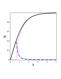
Figure 1: (Color online) The average value of the edge MF as the function of the applied local voltage (magnetic field, tunneling) for $I=1$, $J^{\prime}=J=0$ and $I^{\prime}=1.1$ at $T=0.7$. The dashed (blue) line shows the contribution from extended states, the dotted (red) line describes the contribution from the localized mode, and the solid (black) line is the total value.

So, the presence of the edge MF can be seen from the features of temperature- and $h$-dependent behavior of $M\equiv(1/2)\langle c_{B,0}\rangle$. In fact, we see that the parameter $h$ governs the behavior of the edge MF. For $h=0$ we have $\langle c_{B,0}\rangle=0$ as it must be. For $J^{\prime}=J$ and $I^{\prime}=I$ the localized state exists due to nonzero $h$. Fig. 1 shows the behavior of $M(h)$. The latter is the average value of the edge MF operator for the chain of Josephson junctions as a function of the strength of the local applied voltage, and for the chain of cavities in quantum optics as a function of tunneling/pumping. For the spin chain, $M(h)$ describes the local magnetic moment at the edge of the chain as a function of the local field. At small $h$ the average value is determined by the contribution from the extended (band) states, while at large $h$ it is determined by the localized excitation. The edge MF (as well as the localized state) exists even for $J=J^{\prime}=0$ for $h\neq 0$ (i.e., for Kitaev’s model in the absence of pairing, $\Delta=0$), due to the pairing caused by $h$ itself. For $J=J^{\prime}=0$ at small values of $h$ the average value of the local MF operator shows $M\sim(h/I)|\ln(h/I)|$ behavior. For smaller values of $I^{\prime}$ the region of $h$ appears, in which the contribution of the localized mode is zero. Similar features can be also seen in the behavior of the local susceptibility with respect to $h$, $\chi=\partial M/\partial h$. For instance, temperature dependences of the local susceptibility for several values of the strength of the local applied potential (magnetic field, tunneling) are shown in Fig. 2. At $h=0$ the local susceptibility diverges (for $J=J^{\prime}=0$), while at nonzero $h$ it manifests the non-monotonic temperature behavior: First it grows with $T$ at low temperatures, gets the maximum value (which becomes lower with the growth of $h$), and then decays with temperature.

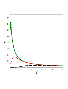
Figure 2: (Color online) The susceptibility of the edge MF $\chi$ as the function of the temperature for $I=1$, $J^{\prime}=J=0$ and $I^{\prime}=1.1$ The dotted (blue) line corresponds to the strength of the applied local voltage (magnetic field, tunneling) $h=0$, the solid (green) line shows $h=0.1$ case, the dashed-dotted (red) line describes $h=0.635$ case (where the contribution from the localized state appears, see Fig. 1), and the dotted (black) line shows $h=3.5$ case.

Such a behavior of the edge MF can be observed in a spin chain with the help of, e.g., nuclear magnetic resonance (NMR). In NMR experiments with spin chains the shift of the resonance position is proportional to the local susceptibility Z . We expect similar results to persist in the case of any spin-1/2 antiferromagnetic chain with the “easy-plane” magnetic anisotropy (with or without in-plane anisotropy, which is important for experimental realization in spin chain materials) with the local magnetic field applied in-plane. For example, spin chain materials with magnetic ions Cu²⁺ or V⁴⁺ (spin 1/2) often exhibit magnetic anisotropy about 5-10 %, and finite spin chains can be realized via substitution of nonmagnetic ions instead of magnetic ones dop . Single crystals of quasi-1d magnetic materials are necessary for the realization of the effect, because in powders spin chains can be directed randomly. The local field can be caused by the proximity effect of a ferromagnet, neighboring to the spin chain, with the value of $h$ governed by the distance to that ferromagnet. One can realize in-plane direction of $h$ by rotation of the ferromagnet. Then the local magnetic susceptibility at the edge of the spin chain can be measured via the NMR shift. Worth noting that Luttinger liquid approach cannot in principle describe localized states, which affect the behavior of edge MF; however, it can describe the low-$h$ behavior, determined by extended states of the chain. For the chain of Josephson junctions such a characteristic can be observed when studying the charge of the edge island as a function of the voltage, applied locally to the edge of the chain vHAHBB , and temperature, or the tunneling Andreev conductance. Finally, in quantum optics the edge MF can be detected by measuring the state of the probe cavity (or the edge cavity) as a function of the tunneling amplitude BT . We expect similar effects for the edge MF on the opposite side of the finite chain. For the extended states of the latter one can replace $k\to\pi q/N+2$ with integer $q$.

In summary, we have proposed the way of direct observation of the edge MF in several realizations in quantum chains, where excitations can be presented as superpositions of spinless fermions and holes, the necessary condition for MF: In “easy-plane” spin-1/2 chains with in-plane polarized magnetic field, applied to the edge of the chain; in the chain of Josephson junctions, and in the chain of cavities in quantum optics with the tunneling of photons to the edge cavity. As we have shown, such an edge MF can be observed at nonzero temperatures in experiments on dc or ac Josephson currents in chains of superconducting islands, nonlinear quantum optics, and quantum spin chain materials, as the local characteristic of the edge under the action of the governing parameter, $h$, which directly affects the edge MF.

Support from the Institute for Chemistry of the V.N. Karasin Kharkov National University is acknowledged.

I Supplemental material

In this Material we present some details of calculation, and some additional features of the behavior of the edge Majorana fermion in the considered systems, as a function of the governing parameter $h$.

Consider of the Hamiltonian ${\cal H}={\cal H}_{0}-hS_{0}^{x}$, where

$${\cal H}_{0}=-\sum_{n=1}^{N}(J_{x}S_{n}^{x}S_{n+1}^{x}+J_{y}S_{n}^{y}S_{n+1}^{y})-J_{x}^{\prime}S_{0}^{x}S_{1}^{x}-J_{y}^{\prime}S_{0}^{y}S_{1}^{y}\ ,$$ (8)

$S_{n}^{x,y}$ are operators of the projections of spin 1/2 situated at the $n$-th site, $J_{x,y}$ are coupling constants, and $J^{\prime}_{x,y}$ are coupling constants for the impurity, situated at the site $n=0$. For simplicity of the consideration let us add the spin $S_{-1}$ at the left edge of the chain with the coupling $-2hS_{0}^{x}S_{-1}^{x}$, so that we study the Hamiltonian ${\cal H}_{M}={\cal H}_{0}-2hS_{0}^{x}S_{-1}^{x}$ instead of ${\cal H}$. The average value $\langle S_{0}^{x}\rangle$ can be written as $\langle S_{0}^{x}\rangle={\rm Tr}(\rho S_{0}^{x})$, where the density matrix is determined as usually $\rho=Z^{-1}\exp((-{\cal H}/T))$, with $Z={\rm Tr}\exp(-{\cal H}/T)$, where $T$ is the temperature. Then it is easy to check that

$${\rm Tr}_{N+1}(\rho S_{0}^{x})={\rm Tr}_{N+2}[\rho_{M}S_{0}^{x}(1+2S_{-1}^{x})]$$

$$\equiv 2{\rm Tr}_{N+2}(\rho_{M}S_{0}^{x}S_{-1}^{x})\ ,$$ (9)

where we used the subscripts $N+1$ and $N+2$ to emphasize that the traces are taken with respect to eigenstates of the system consisting of $N+1$ or $N+2$ spins, respectively, and $\rho_{M}=Z_{M}^{-1}\exp(-{\cal H}_{M}/T)$, where $Z_{M}={\rm Tr}\exp(-{\cal H}_{M}/T)$. The last equality uses the fact that the average of the operator, linear in $S_{0}^{x}$, with the Hamiltonian, quadratic in operators of $S^{x}_{n}$ and $S_{n}^{y}$, is zero.

To find eigenfunctions and eigenvalues of the system with the Hamiltonian ${\cal H}_{M}$, we use the Jordan-Wigner transformation to fermion operators,

$$S_{m}^{\pm}=S_{m}^{x}\pm iS_{m}^{y}\ ,\ S_{m}^{z}\equiv{\sigma_{m}\over 2}={1\over 2}-d_{m}^{\dagger}d_{m}\ ,$$

$$S_{m}^{+}=\prod_{n=-1}^{m-1}\sigma_{n}d_{m}\ ,\ S_{m}^{-}=d_{m}^{\dagger}\prod_{n=-1}^{m-1}\sigma_{m}\ ,$$

(10)

with $d^{\dagger}_{m}$ ($d_{m}$) being standard Dirac creation (destruction) fermionic operator $\{d^{\dagger}_{m},d^{\dagger}_{n}\}=\{d_{m},d_{n}\}=0$, $\{d_{m},d_{n}^{\dagger}\}=\delta_{mn}$, where the anticommutator is determined as $\{X,Y\}=XY+YX$. In that representation we have

$${\cal H}_{M}=-{1\over 2}\biggl{(}h[d_{-1}^{\dagger}d_{0}+d_{-1}^{\dagger}d_{0}^{\dagger}+{\rm h.c.}]$$

$$+I^{\prime}[d_{1}^{\dagger}a_{0}+d_{0}^{\dagger}a_{1}]+J^{\prime}[d_{1}^{\dagger}d_{0}^{\dagger}+d_{0}d_{1}]$$

$$+\sum_{n=1}^{N-1}[I(d_{n}^{\dagger}d_{n+1}+d_{n+1}^{\dagger}d_{n})$$

$$+J(d_{n}^{\dagger}d_{n+1}^{\dagger}+d_{n+1}d_{n})]\biggr{)}\ .$$ (11)

Then we use the unitary transformation

$$d_{n}=\sum_{\lambda}(u_{n,\lambda}d_{\lambda}+v_{n,\lambda}d_{\lambda}^{\dagger})\ ,$$ (12)

where $\lambda$’s are quantum numbers, which parameterize all eigenstates of the diagonalized Hamiltonian. These quantum numbers can describe extended (band) states. Besides, there is a possibility of localized states, caused by $h\neq 0$, $I^{\prime}\neq I$, and $J^{\prime}\neq J$. Let us define $P_{n,\lambda},Q_{n,\lambda}=u_{n,\lambda}\pm v_{n,\lambda}$, i.e., transfer to Majorana modes $d_{n}=(1/2)\sum_{\lambda}(P_{n,\lambda}c_{B,\lambda}-iQ_{n,\lambda}c_{A,\lambda})$.

Then we can write the stationary Schrödinger equation with ${\cal H}_{M}$ in the co-ordinate space. From that equation for $n=2,3,\dots$ we have

$$2\varepsilon P_{n}+(I-J)Q_{n+1}+(I+J)Q_{n-1}=0\ ,$$

$$2\varepsilon Q_{n}+(I+J)P_{n+1}+(I-J)P_{n-1}=0\ ,$$ (13)

where $\varepsilon$ are the energies (we drop subscripts $\lambda$ for simplicity). On the other hand, for the sites $n=0,1,-1$ we have two sets of equations, different from Eqs. (13). The one, which depends on $h$, is

$$2\varepsilon Q_{1}+(I+J)P_{2}+(I^{\prime}-J^{\prime})P_{0}=0\ ,$$

$$2\varepsilon P_{0}+(I^{\prime}-J^{\prime})Q_{1}+2hQ_{-1}=0\ ,$$

$$\varepsilon Q_{-1}+hP_{0}=0\ ,$$ (14)

and the one, which does not depend on $h$, is

$$2\varepsilon P_{1}+(I-J)Q_{2}+(I^{\prime}+J^{\prime})Q_{0}=0\ ,$$

$$2\varepsilon Q_{0}+(I^{\prime}+J^{\prime})P_{1}=0\ ,$$

$$\varepsilon P_{-1}=0\ .$$ (15)

We have two disconnected systems of equations in finite differences. It has two sets of eigenfunctions. The first set of solutions describes nonzero $P_{n,\lambda}$ for even $n$, and nonzero $Q_{n,\lambda}$ for odd $n$ (all other $P$’s and $Q$’s are zeros). The second set of solutions describes nonzero $P_{n,\lambda}$ for odd $n$, and nonzero $Q_{n,\lambda}$ for even $n$ (others are zeros). For each set we look for extended (band) states with $\lambda\to k$, where $k$ is the quasimomentum of the eigenstate, and for a localized state, which wave function decays exponentially with the distance from the edge of the chain.

The solution of Eqs. (14) and (15) is as follows. For the extended states (with quasimomenta $k\equiv\lambda$ in the limit $N\to\infty$) we get ($m\neq 0$)

$$Q_{2m-1,k}^{(1)}=-\frac{2}{\sqrt{\pi}x_{k}^{(1)}\varepsilon_{k}}([\varepsilon_{k}^{2}-h^{2}][(I^{2}-J^{2})\sin(2km)$$

$$+(I-J)^{2}\sin[2k(m-1)]]$$

$$-\varepsilon_{k}^{2}(I^{\prime}-J^{\prime})^{2}\sin[2k(m-1)])\ ,$$

$$P_{2m,k}^{(1)}=\frac{2}{\sqrt{\pi}x_{k}^{(1)}}[2(\varepsilon_{k}^{2}-h^{2})(I-J)\sin(2km)$$

$$-(I^{\prime}-J^{\prime})^{2}(I\cos k\sin[k(2m-1)]$$

$$-J\sin k\cos[k(2m-1)])]\ .$$ (16)

For $m=0$ we obtain $Q_{-1,k}^{(1)}=-hP_{0,k}^{(1)}/\varepsilon_{k}$ and

$$P_{0,k}^{(1)}=\frac{2}{\sqrt{\pi}x_{k}^{(1)}}(I^{2}-J^{2})(I^{\prime}-J^{\prime})\sin k\cos k\ ,$$ (17)

Here we use the following notation

$$x_{k}^{(1)}=|2(\varepsilon_{k}^{2}-h^{2})(I-J)-(I^{\prime}-J^{\prime})^{2}(I\cos k+iJ\sin k)e^{ik}|\ .$$ (18)

The energies of extended states are $\varepsilon_{k}^{2}=I^{2}\cos^{2}k+J^{2}\sin^{2}k$. For the localized state (with $|r_{(1)}|<1$) we get ($m\neq 0$)

$$P_{2m}^{(1)}=P_{0}\frac{(I^{\prime}-J^{\prime})}{(I-J)}r_{(1)}^{2m}\ ,$$

$$Q_{2m-1}^{(1)}=-P_{0}\frac{(I^{\prime}-J^{\prime})}{(I-J)}$$

$$\times\frac{(I+J)r_{(1)}+(I-J)r^{-1}_{(1)}}{2\varepsilon_{(1)}}r_{(1)}^{2m-1}\ ,$$ (19)

For $m=0$ the localized eigenstates are $P_{0}^{(1)}=P_{0}$, $Q_{-1}^{(1)}=-P_{0}h/\varepsilon_{(1)}$. The parameter $r_{(1)}$ ($\ln(r_{(1)})$ is the localization radius) is

$$r_{(1)}^{2}=\frac{(I-J)}{2(I+J)[(I-J)^{2}-(I^{\prime}-J^{\prime})^{2}]}$$

$$\times\biggl{(}4h^{2}+(I^{\prime}-J^{\prime})^{2}-2(I^{2}+J^{2})$$

$$-[(2h-I-J)^{2}+(I^{\prime}-J^{\prime})^{2}-(I-J)^{2}]^{1/2}$$

$$\times[(2h+I+J)^{2}+(I^{\prime}-J^{\prime})^{2}-(I-J)^{2}]^{1/2}\biggr{)}\ .$$ (20)

This state exists if $[(2h-I-J)^{2}+(I^{\prime}-J^{\prime})^{2}-(I-J)^{2}][(2h+I+J)^{2}+(I^{\prime}-J^{\prime})^{2}-(I-J)^{2}]>0$. Notice that $|r_{(1)}|<1$, i.e., localized state decays with the distance from the edge of the chain. Even for the homogeneous case $I^{\prime}=I$, $J^{\prime}=J$ for $I+3J>0$ such a localized mode exists at $h\neq 0$. For the second set of extended states we have ($m\neq 0$)

$$Q_{2m,k}^{(2)}=\frac{2}{\sqrt{\pi}x_{k}^{(2)}}[2\varepsilon_{k}^{2}(I+J)\sin(2km)$$

$$-(I^{\prime}+J^{\prime})^{2}(I\cos k\sin[k(2m-1)]$$

$$+J\sin k\cos[k(2m-1)])]\ ,$$

$$P_{2m-1,k}^{(2)}=-\frac{2\varepsilon_{k}}{\sqrt{\pi}x_{k}^{(2)}}[(I^{2}-J^{2})\sin(2km)$$

$$+[(I+J)^{2}-(I^{\prime}+J^{\prime})^{2}]\sin[2k(m-1)]]\ .$$ (21)

For $m=0$ we obtain $P_{-1,k}^{(2)}=0$ and

$$Q_{0,k}^{(2)}=\frac{2}{\sqrt{\pi}x_{k}^{(2)}}(I^{2}-J^{2})(I^{\prime}+J^{\prime})\sin k\cos k\ .$$ (22)

Here we use

$$x_{k}^{(2)}=|2\varepsilon_{k}^{2}(I+J)-(I^{\prime}+J^{\prime})^{2}(I\cos k-iJ\sin k)e^{ik}|\ .$$ (23)

For the second set of localized states ($|r_{(2)}|<1$) we obtain ($m\neq 0$)

$$Q_{2m}^{(2)}=Q_{0}\frac{(I^{\prime}+J^{\prime})}{(I+J)}r_{(2)}^{2m}\ ,$$

$$P_{2m-1}^{(2)}=-Q_{0}\frac{(I^{\prime}+J^{\prime})}{(I+J)}$$

$$\times\frac{(I-J)r_{(2)}+(I+J)r^{-1}_{(2)}}{2\varepsilon_{(2)}}r_{(1)}^{2m-1}\ ,$$ (24)

while for $m=0$ the solution has the form $Q_{0}^{(2)}=Q_{0}$, $P_{-1}^{(2)}=0$. We use

$$P_{0},Q_{0}=\left[\left(\frac{(I^{\prime}\mp J^{\prime})}{(I\mp J)}\right)^{2}\frac{r^{4}_{(1,2)}}{1-r^{4}_{(1,2)}}+1\right]^{-1/2},\$$

$$r_{(2)}^{2}=\frac{(I^{2}-J^{2})}{[(I^{\prime}+J^{\prime})^{2}-(I-J)^{2}]}\ .$$ (25)

For $I^{\prime}=I$ and $J^{\prime}=J$ there is no second localized state. The energies of the localized states are

$$4\varepsilon_{(1,2)}^{2}=I^{2}[r_{(1,2)}+r^{-1}_{(1,2)}]^{2}-J^{2}[r_{(1,2)}-r^{-1}_{(1,2)}]^{2}$$ (26)

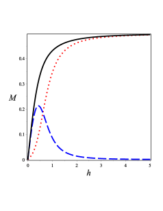
Figure 3: (Color online) The average value of the edge Majorana fermion $M\equiv(1/2)\langle c_{B,0}\rangle$ as the function of the strength of the applied local voltage (magnetic field, tunneling) $h$ for $I=1$, $J^{\prime}=J=0$ and $I^{\prime}=1.5$ at $T=0.1$. The dashed (blue) line shows the contribution from extended states, the dotted (red) line describes the contribution from the localized mode, and the solid (black) line is the total value.

Here we also present several figures which describe the behavior of the average value for the edge Majorana fermion operator $M\equiv(1/2)\langle c_{B,0}\rangle=\langle S_{0}^{x}\rangle$ and its local susceptibility $\chi=\partial M/\partial h$ for the considered quantum chains.

Fig. 3 shows the behavior of $M(h)$ for large enough impurity coupling $I^{\prime}=1.5I$ at low temperatures.

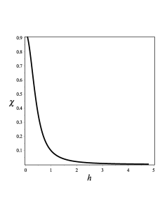
Figure 4: The behavior of the local susceptibility $\chi(h)$ for the situation of Fig. 3 at low temperatures $T=0.1$.

Fig. 4 shows $\chi(h)$ for such a case.

Fig. 5 presents the behavior of the average value $M(h)$ for the homogeneous case $I^{\prime}=I$ ($J^{\prime}=J=0$) at low temperatures and high temperatures.

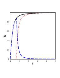
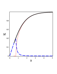
Figure 5: (Color online) The average value of the edge Majorana fermion $M\equiv(1/2)\langle c_{B,0}\rangle$ as the function of the strength of the applied local voltage (magnetic field, tunneling) $h$ for the homogeneous chain $I=I^{\prime}=1$, $J^{\prime}=J=0$ at $T=0.1$ (top) and $T=0.8$ (bottom). The dashed (blue) line shows the contribution from extended states, the dotted (red) line describes the contribution from the localized mode, and the solid (black) line is the total value.

The reader can see that no principal difference between the homogeneous and non-homogeneous cases exists. The upper panel of Fig. 5 manifests the behavior of $M(h)$ for the homogeneous case at low temperatures, $T=0.1I$. The lower panel of Fig. 5 manifests the behavior of $M(h)$ for the same homogeneous case but at high temperatures, $T=0.8I$.

The behavior of the susceptibility $\chi(h)$ for the homogeneous chain at low temperatures $T=0.1I$ and at high temperatures $T=0.8I$ are presented in Fig. 6.

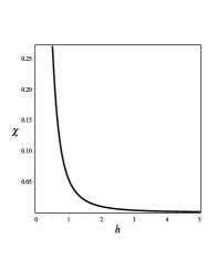
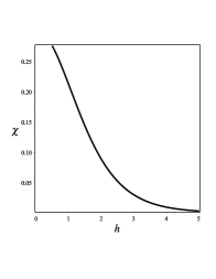
Figure 6: The behavior of the local susceptibility $\chi(h)$ of the homogeneous chain like in Fig. 5 at low temperatures $T=0.1I$ (top) and at high temperatures $T=0.8I$ (bottom).

As expected, lower values of the temperature yield sharper behavior of the susceptibility at small values of $h$. Finally, Fig. 7 shows the temperature behavior of the local magnetic susceptibility for the chain with $I=1$, $J=0.5$, $I^{\prime}=1.5$ and $J^{\prime}=0.6$ for several values of the applied local field (voltage, tunneling).

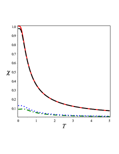
Figure 7: (Color online) The susceptibility of the edge Majorana fermion $\chi$ as the function of the temperature for several values of the strength of the applied local voltage (magnetic field, tunneling) $h$ for the chain with $I=1$, $J=0.5$, $I^{\prime}=1.5$ and $J^{\prime}=0.6$. The solid (red) line describes the case $h=0$; the dashed (black) line shows $h=0.1$ case; the dotted (blue) line describes the case $h=1$, and the dashed-dotted (green) line shows $h=2$ case.

One can see that $J\neq 0$ and/or $J^{\prime}\neq 0$ (which is related to the biaxial magnetic anisotropy in the spin system, or nonzero pairing in the toy Kitaev model) removes the $h\to 0$ divergency of the local susceptibility of the edge Majorana mode. Also, for the cases with nonzero $J$ and/or $J^{\prime}$ the temperature behavior of $\chi(T)$ is almost monotonic: $\chi$ is finite at low temperatures and decays with the growth of $T$.

References

(1) F. Wilczek, Nature Physics 5, 614 (2009).
(2) D.A. Ivanov, Phys. Rev. Lett. 86, 268 (2001);
S. Das Sarma, M. Freedman, and C. Nayak, ibid.94, 166802 (2005)
A.Yu. Kitaev, Ann.Phys.(NY) 303, 2 (2003).
(3) A.Yu. Kitaev, Phys. Usp. 44, 131 (2001).
(4) N. Read and D. Green, Phys. Rev. B 61, 10267 (2000);
N.B. Kopnin and M.M. Salomaa, Phys. Rev. B 44, 9667 (1991).
(5) J. Alicea, Rep. Progr. Phys. 75, 076501 (2012);
C.W.J. Beenakker, Annu. Rev. Condens. Matter Phys. 4, 113 (2013); T.D. Stanescu and S. Tewari,
arXiv:1302.5433 (2013).
(6) L. Fu and C.L. Kane, Phys. Rev. Lett. 100, 096407 (2008);
Phys. Rev. B 79, 161408(R) (2009).
(7) R.M. Lutchyn, J.D. Sau, and S. Das Sarma, Phys. Rev. Lett.
105, 077001 (2010); Y. Oreg, G. Refael, and F. von Oppen, Phys. Rev.
Lett. 105, 177002 (2010).
(8) V. Mourik et al.,
Science 336, 6084 (2012); A. Das et al.,
Nature Phys. 8, 887 (2012); M.T. Deng et al.,
Nano Lett. 12, 6414 (2012); L.P. Rokhinson, X. Liu, and J.F. Furdyna,
Nature Phys. 8, 795 (2012); J.G. Rodrigo et al.,
arXiv:1302.0598 (2013).
(9) J. Liu et al.,
Phys. Rev. Lett. 109, 267002 (2012); E.J.H. Lee et al.,
Phys. Rev. Lett. 109, 186802 (2012); D.I. Pikulin et al.,
New J. Phys. 14, 125011 (2012).
(10) V.Z. Kleiner and V.M. Tsukernik, Fiz. Nizk. Temp. 6, 332
(1980) (in Russian) [Sov. J. Low Temp. Phys. 6, 158 (1980)]; V.Z. Kleiner, Ph.D. thesis ILTPE, Kharkov, (unpublished) (1982).
(11) See, e.g., A.A. Zvyagin Finite-Size Effects in Correlated
Electron Systems: Exact Results, Imperial College Press, London, 2005, and
references therein.
(12) E.H. Lieb, T.D. Schultz, and D.C. Mattis, Ann. Phys. 16, 407
(1961).
(13) C.-E. Bardyn and A. Imamoglu, Phys. Rev. Lett. 109,
253606 (2012); I. Carusotto
et al., Phys. Rev. Lett. 103 033601 (2009).
(14) B. van Heck, F. Hassler, A.R. Akhmerov, and
C.W.J. Beenakker, Phys. Rev. B 84, 180502(R) 2011; B. van Heck
et al.,
New J. Phys. 14, 035019 (2012); F. Hassler and D. Schuricht,
New J. Phys. 14, 125018 (2012).
(15) See, e.g., A.A. Zvyagin, Phys. Rev. B 85, 134435 (2012)
and references therein.
(16) See, e.g, V. Kataev et al.,
Phys. Rev. Lett. 86, 2882 (2001); K.M. Kojima et al., Phys. Rev. B
70, 094402 (2004); R. Klingeler et al.,
Phys. Rev. B 72, 184406 (2005).