Kondo effect in the Kohn-Sham conductance of multiple levels quantum dots

Abstract

At zero temperature, the Landauer formalism combined with static density functional theory is able to correctly reproduce the Kondo plateau in the conductance of the Anderson impurity model provided that an exchange-correlation potential is used which correctly exhibits steps at integer occupation.

Here we extend this recent finding to multi-level quantum dots described by the constant-interaction model. We derive the exact exchange-correlation potential in this model for the isolated dot and deduce an accurate approximation for the case when the dot is weakly coupled to two leads. We show that at zero temperature and for non-degenerate levels in the dot we correctly obtain the conductance plateau for any odd number of electrons on the dot. We also analyze the case when some of the levels of the dot are degenerate and again obtain good qualitative agreement with results obtained with alternative methods.

As in the case of a single level, for temperatures larger than the Kondo temperature, the Kohn-Sham conductance fails to reproduce the typical Coulomb blockade peaks. This is attributed to dynamical exchange-correlation corrections to the conductance originating from time-dependent density functional theory.

1 Introduction

Common wisdom has it that Density Functional Theory (DFT) is not able to describe strongly correlated systems although the fundamental theorems of DFT apply to these systems as well. In fact, the difficulties of dealing with strong correlations are not inherent to DFT but to the DFT approximations. In the last years there has been considerable progress in understanding which features a DFT approximation should have in order to capture strong correlation effects [1, 2, 3, 4, 5, 6, 7, 8, 9, 10, 11, 12, 13], and the derivative discontinuity of the exchange-correlation energy functional [14] has emerged as one of the key properties. In the context of quantum transport the derivative discontinuity turned out to be crucial to reproduce the conductance plateau [15, 16, 17] due to the Kondo effect, a hallmark of strong correlations. In this paper we extend the analysis of Ref. [15] to multiple levels and finite temperature. In particular we investigate the reliability of the exact Kohn-Sham (KS) conductance in multi-level quantum-dot systems. The paper is organized as follows. In Section 2 we introduce the Constant Interaction Model (CIM) for the description of a multi-level quantum dot, and derive the exact xc potential of the isolated dot as well as an approximate, but accurate, xc potential for the dot coupled to leads. In Section 3 we discuss the self-consistent DFT equations of the CIM and how to calculate the KS conductance at finite bias and temperature. Results on different quantum dots are presented in Section 4. Our main findings are that (i) the zero-temperature KS conductance correctly exhibits plateaus of height $nG_{0}$ where $G_{0}=2e^{2}/h$ is the quantum of conductance and $n=1,\ldots,g$, with $g$ the degeneracy of the levels, (ii) if only $g^{\prime}<g$ degenerate levels are coupled to the leads then the height of the plateaus does not exceed $g^{\prime}G_{0}$ and the length of the plateau of height $g^{\prime}G_{0}$ is $[2(g-g^{\prime})+1]$ times the charging energy. and (iii) the finite temperature KS conductance seriously overestimates the true conductance at temperatures higher than the Kondo temperature. We summarize and draw our conclusions in Section 5.

2 The xc potential in the constant interaction model

A popular model of quantum dots is the Constant Interaction Model (CIM) described by the Hamiltonian

$$\hat{H}_{\rm QD}=\hat{H}_{0}+\hat{H}_{\rm int}$$ (1)

where the non-interacting part of the Hamiltonian is $\hat{H}_{0}=\sum_{l}\epsilon_{l}\hat{c}_{l}^{\dagger}\hat{c}_{l}$. The $\epsilon_{l}$ are the single-particle eigenvalues of $\hat{H}_{0}$ (the quantum number $l=i\sigma$ comprises an orbital, $i$, and a spin, $\sigma$, degree of freedom) and, for future reference, $\phi_{l}$ are the corresponding single-particle orbitals. The interaction has the simple form[18]

$$\hat{H}_{\rm int}=\frac{1}{2}E_{C}(\hat{N}-N_{0})^{2}$$ (2)

where $E_{C}$ is the charging energy, $\hat{N}=\sum_{l}\hat{c}_{l}^{\dagger}\hat{c}_{l}$ is the operator for the total number of electrons and $N_{0}$ is the number of electrons in the charge neutral state. Since $\hat{H}_{\rm int}$ depends only on $\hat{N}$, and $\hat{N}$ commutes with $\hat{H}_{0}$, the eigenstates of $\hat{H}_{0}$ are also eigenstates of $\hat{H}_{\rm QD}$:

$$\hat{H}_{0}|\Psi\rangle=E_{0}|\Psi\rangle\quad\Rightarrow\quad\hat{H}_{\rm QD}|\Psi\rangle=E|\Psi\rangle$$ (3)

with

$$E=E_{0}+\frac{1}{2}E_{C}(N-N_{0})^{2}$$ (4)

and $\hat{N}|\Psi\rangle=N|\Psi\rangle$. Therefore the eigenstates of $\hat{H}_{\rm QD}$ with $N$ electrons are Slater determinants of $N$ occupied single-particle eigenfunctions $\phi_{l_{1}},\ldots,\phi_{l_{N}}$ and have eigenvalue $E=\epsilon_{l_{1}}+\ldots\epsilon_{l_{N}}+\frac{1}{2}E_{C}(N-N_{0})^{2}$.

The KS system of the CIM is described by the KS Hamiltonian

$$\hat{H}_{\rm KS}=\hat{H}_{0}+\int d{\mathbf{r}}\;v_{\rm Hxc}({\mathbf{r}})\hat{n}({\mathbf{r}})$$ (5)

where $v_{\rm Hxc}$ is the Hartree-xc potential and $\hat{n}$ is the density operator whose integral over all space gives the operator $\hat{N}$. The Hartree-xc potential is a universal functional of the density, $v_{\rm Hxc}=v_{\rm Hxc}[n]$, and has the property that for a given temperature $T$ and chemical potential $\mu$ the equilibrium density of $\hat{H}_{\rm QD}$ and $\hat{H}_{\rm KS}$ are identical. Note that we are using the finite-temperature (or ensemble) DFT as formulated in Ref. [19], thus there is no ambiguity in $v_{\rm Hxc}$ with respect to addition of a constant since the number of particles can fluctuate.

Let us consider the quantum dot at zero temperature and denote by $E(N)$ the ground-state energy of $\hat{H}_{\rm QD}$ with $N$ electrons. For a given $\mu$ the number of electrons $N$ is the largest integer for which the addition energy

$$A(N)\equiv E(N)-E(N-1)<\mu.$$ (6)

The ground state of $\hat{H}_{\rm QD}$ with $N$ electrons has, in general, degeneracy $d$ and therefore the zero-temperature density can be written as

$$n({\mathbf{r}})=\frac{1}{d}\sum_{j=1}^{d}\langle\Psi_{j}|\hat{n}({\mathbf{r}})|\Psi_{j}\rangle$$ (7)

where $|\Psi_{j}\rangle$ is the $j$-th component of the ground-state multiplet. Since every $|\Psi_{j}\rangle$ is a Slater determinant the generic term of the sum in Eq. (7) has the form

$$\langle\Psi_{j}|\hat{n}({\mathbf{r}})|\Psi_{j}\rangle=\sum_{k=1}^{N}|\phi^{(j)}_{l_{k}}({\mathbf{r}})|^{2}$$ (8)

where the $\phi^{(j)}_{l_{k}}$’s are the eigenfunctions of the Slater determinant $\Psi_{j}$. We now show that for the KS system to reproduce the same density of the interacting system the Hartree-xc potential has to be uniform in space and depend only on the total number of particles, i.e.,

$$v_{\rm Hxc}[n]({\mathbf{r}})=v_{\rm Hxc}[N].$$ (9)

Interestingly the fact that $v_{\rm Hxc}$ is uniform in space is not an exclusive feature of systems invariant under translations, like the electron gas. In the CIM Hamiltonian the one-body part $\hat{H}_{0}$ can be any; the uniformity of $v_{\rm Hxc}$ is due to the fact that $\hat{H}_{\rm int}$ depends only on $\hat{N}$. To prove Eq. (9) we simply observe that if $v_{\rm Hxc}$ is independent of ${\mathbf{r}}$ then the KS eigenfunctions are identical to the single-particle eigenfunctions $\phi_{l}$ and hence the KS density is again given by Eq. (7) provided that $N$ is the largest integer for which the KS eigenvalue

$$\epsilon_{H(N)}+v_{\rm Hxc}[N]<\mu.$$ (10)

In Eq. (10) $\epsilon_{H(N)}$ is the noninteracting energy of the HOMO level with $N$ electrons; if we order the single-particle energies according to $\epsilon_{1}\leq\epsilon_{2}\leq\epsilon_{3}\leq\ldots$ then $\epsilon_{H(N)}=\epsilon_{N}$. It is easy to show that for any real $N$ the explicit form of $v_{\rm Hxc}$ is

$$v_{\rm Hxc}[N]=A(\bar{N})-\epsilon_{\bar{N}},\quad\quad\bar{N}\equiv{\rm Int}[N]$$ (11)

where $\bar{N}$ is the integer part of $N$. Suppose that there are $\bar{N}$ electrons in the quantum dot so that $A(\bar{N})<\mu<A(\bar{N}+1)$. Then $\epsilon_{\bar{N}}+v_{\rm Hxc}[\bar{N}]=A(\bar{N})<\mu$ whereas $\epsilon_{\bar{N}+1}+v_{\rm Hxc}[\bar{N}+1]=A(\bar{N}+1)>\mu$; hence $\bar{N}$ is the largest integer for which Eq. (10) is fulfilled. Taking into account the explicit form of the interaction we have

$$A(\bar{N}) = \epsilon_{\bar{N}}+\frac{1}{2}E_{C}(\bar{N}-N_{0})^{2}-\frac{1}{2}E_{C}(\bar{N}-1-N_{0})^{2}$$ (12)

$$= \epsilon_{\bar{N}}+E_{C}(\bar{N}-N_{0}-\frac{1}{2})$$

and from Eq. (11) we deduce that

$$v_{\rm Hxc}[N]=E_{C}\bar{N}-E_{C}(N_{0}+\frac{1}{2}).$$ (13)

Thus the Hartree-xc potential of the CIM is piece-wise constant with discontinuities $E_{C}$ every time $N$ crosses an integer. One can verify that the size of the discontinuities coincides with the xc part of the derivative discontinuity of the ground states energy, as it should be. We mention that there exists generalizations of the CIM with $\bar{N}$-dependent discontinuities [20] for which an analytic expression of the Hartree-xc potential can still be derived [21].

Next we discuss how to account for the effects of the coupling between the quantum dot and the leads. We consider a left ($L$) and a right ($R$) lead with Hamiltonian

$$\hat{H}_{\rm lead}=\sum_{k\alpha}\epsilon_{k\alpha}\hat{c}^{{\dagger}}_{k\alpha}\hat{c}_{k\alpha}$$ (14)

where the operators $c_{k\alpha}$ ($c^{{\dagger}}_{k\alpha}$) annihilate (create) an electron of energy $\epsilon_{k\alpha}$ in lead $\alpha=L,R$. In the following we assume that the band-width of the leads is much larger than any other energy scale and that the quantum-dot energies $\epsilon_{l}$ are all well inside the leads band. This is the Wide Band Limit Approximation (WBLA). The contact between the leads and the quantum dot is described by the tunneling Hamiltonian

$$\hat{H}_{\rm T}=\sum_{k\alpha}\sum_{l}T_{k\alpha,l}c^{{\dagger}}_{k\alpha}\hat{c}_{l}+{\rm H.c.}$$ (15)

For a single-level quantum dot, $l=1$, the full Hamiltonian $\hat{H}=H_{\rm QD}+\hat{H}_{\rm T}+\hat{H}_{\rm lead}$ reduces to the Hamiltonian of the Anderson model. In this case one can show that due to the dot-lead coupling the sharp steps of the Hartree-xc potential are smeared. In particular the derivative $\partial v_{\rm Hxc}/\partial N$ at $N=1$ is not infinite but instead given by $\pi E_{C}^{2}/4\gamma$ [22], where $\gamma$ is the contact-induced broadening of the spectral function

$$\gamma=2\pi\sum_{k\alpha}|T_{k\alpha,1}|^{2}\delta(\omega-\epsilon_{k\alpha})$$ (16)

which is $\omega$-independent in the WBLA. Using the Bethe Ansatz [23] it is possible to extract the exact form of $v_{\rm Hxc}$ by reverse engineering [16] and show that it is well approximated by (modulo an additive constant)

$$v_{\rm Hxc}[N]=\frac{1}{\pi}E_{C}\arctan\left(\frac{N-1}{W}\right)$$ (17)

where $W$ is a parameter that controls the smearing of the step. Since $\partial v_{\rm Hxc}/\partial N\sim E_{C}^{2}/\gamma$ for $N=1$ (see discussion above Eq. (16)) we have $W\sim\gamma/E_{C}$. The sharp step is recovered in the limit $\gamma\rightarrow 0$, which corresponds to the isolated quantum dot. As the only effect of the dot-lead coupling is to smear the steps of $v_{\rm Hxc}$ we can easily generalize Eq. (17) to multiple-level quantum dots by summing over all charged states [24]

$$v_{\rm Hxc}[N]=\frac{1}{\pi}E_{C}\sum_{l}\arctan\left(\frac{N-l}{W(l)}\right)+C,$$ (18)

where the constant $C$ is chosen such that $v_{\rm Hxc}[0]=0$. $W(l)$ accounts for the smearing of the steps and, in general, depends on $l$. A practical way to estimate the $W(l)$’s consists in constructing the broadening matrix

$$\Gamma_{ll^{\prime}}=2\pi\sum_{k\alpha}T^{\ast}_{k\alpha,l}T_{k\alpha,l^{\prime}}\delta(\omega-\epsilon_{k\alpha})$$ (19)

which is $\omega$-independent in the WBLA, and then take

$$W(l)=\alpha\Gamma_{ll}/E_{C}$$ (20)

with $\alpha$ a constant of order 1. This choice agrees with the $W$ of the Anderson model in the case of a single level. The appealing feature of the smeared Hartree-xc potential in Eq. (18) is that in the limit of weak dot-lead coupling $\Gamma_{ll}\rightarrow 0$, hence $W(l)\rightarrow 0$ and $v_{\rm Hxc}$ correctly reduces (modulo an additive constant) to the Hartree-xc potential of the isolated quantum dot derived in Eq. (13).

Finally we discuss temperature effects. Thermal fluctuations cause a further smearing of the steps in $v_{\rm Hxc}$. However, if we are interested in temperatures $T<{\rm min}[\{\Gamma_{ll}\}]$ the thermal smearing is negligible compared to the smearing induced by the dot-lead coupling [15, 22]. In the remainder of the paper we focus on this low temperature regime and use the Hartree-xc potential of Eq. (18) with the $W$’s from Eq. (20) to calculate the density and the KS conductance.

3 Kohn-Sham density and conductance

Due to the fact that $v_{\rm Hxc}$ is uniform in space the KS Hamiltonian of the quantum dot is diagonal in the basis $\phi_{l}$ which diagonalizes $\hat{H}_{0}$:

$$\hat{H}_{\rm KS}=\sum_{l}(\epsilon_{l}+v_{\rm Hxc}[N])\hat{c}^{{\dagger}}_{l}\hat{c}_{l}.$$ (21)

Let $h_{\rm KS}$ be the single-particle Hamiltonian matrix with matrix elements $[h_{\rm KS}]_{ll^{\prime}}=\delta_{ll^{\prime}}(\epsilon_{l}+v_{\rm Hxc}[N])$ in the basis $\phi_{l}$. The KS retarded Green’s function for the quantum dot in contact with the leads can be written as

$$\mbox{$\mathcal{G}$}_{s}(\omega)=\frac{1}{\omega-h_{\rm KS}+i\Gamma/2}$$ (22)

where the broadening matrix has been defined in Eq. (19). To deal with out-of-equilibrium situations we split $\Gamma=\Gamma_{L}+\Gamma_{R}$ into the sum of the left and right contribution. If we apply a bias $V_{\alpha}$ on lead $\alpha$ and the system attains a steady state in the long-time limit then the steady-state value of the total number of electrons in the quantum dot is given by

$$N=\sum_{\alpha}\int\frac{d\omega}{2\pi}f_{\alpha}(\omega){\rm Tr}\left[\mbox{$\mathcal{G}$}_{s}(\omega)\Gamma_{\alpha}\mbox{$\mathcal{G}$}_{s}^{{\dagger}}(\omega)\right]$$ (23)

where $f_{\alpha}(\omega)=1/(e^{\beta(\omega-V_{\alpha}-\mu)}+1)$ is the Fermi function at inverse temperature $\beta=1/T$ and the symbol ${\rm Tr}$ signifies a trace over all single-particle states of the quantum dot. Since $h_{\rm KS}=h_{\rm KS}[N]$ is a function of $N$, Eq. (23) has to be solved self-consistently. With the steady-state value of $N$ the current of the KS system can be calculated using the Landauer formula [25, 26, 27] (the KS electrons are effectively noninteracting)

$$I=\int\frac{d\omega}{2\pi}[f_{L}(\omega)-f_{R}(\omega)]{\rm Tr}\left[\mbox{$\mathcal{G}$}_{s}(\omega)\Gamma_{L}\mbox{$\mathcal{G}$}_{s}^{{\dagger}}(\omega)\Gamma_{R}\right]$$ (24)

where $\mbox{$\mathcal{G}$}_{s}$ is evaluated at the self-consistent value of $N$. The current $I=I(V_{L},V_{R})$ is a function of $V_{L}$ and $V_{R}$ and correctly vanishes for $V_{L}=V_{R}$. We are interested in the zero-bias conductance which is defined as

$$G_{s}=\left.\frac{dI(V/2,-V/2)}{dV}\right|_{V=0}.$$ (25)

The procedure outlined above is, in essence, the Non-Equilibrium Green’s Functions (NEGF) DFT approach to quantum transport [28, 29, 30, 31, 32]. The theorems of DFT guarantee that the equilibrium density is exact (provided that the exact $v_{\rm Hxc}$ is used) but they do not say anything about out-of-equilibrium situations. In this sense, the NEGF-DFT approach may be viewed as an empirical approach. The rigorous treatment of out-of-equilibrium situations requires to formulate the quantum transport problem within Time-Dependent (TD) DFT [33]. This leads to a correction to Eqs. (23) and (24) in which $V_{\alpha}\rightarrow V_{\alpha}+V_{\alpha,\rm xc}$ where $V_{\alpha,\rm xc}$ is the steady-state value of the TDDFT xc potential in lead $\alpha$ [34, 35, 36]. In the limit of zero bias, $V_{\alpha,\rm xc}$ vanishes but $dV_{\alpha,\rm xc}/dV$, in general, does not [37, 38, 39, 40], and leads to a dynamical correction to the conductance. Adiabatic approximations to the TDDFT $v_{\rm Hxc}$, including the exact DFT Hartree-xc potential [41, 42], do not capture this correction since $V_{\alpha,\rm xc}$ is identically zero in this case. Thus the NEGF-DFT approach corresponds to the solution of the TDDFT equations in the long-time limit and in the adiabatic approximation. This has been nicely confirmed in Refs. [43, 44]. In the next section we investigate the performance of the NEGF-DFT approach in quantum dots using a DFT $v_{\rm Hxc}$, Eq. (18), which is essentially exact in the weak coupling limit. The analysis will help us to understand strengths and limitations of adiabatic approximations in quantum transport.

4 Results and discussions

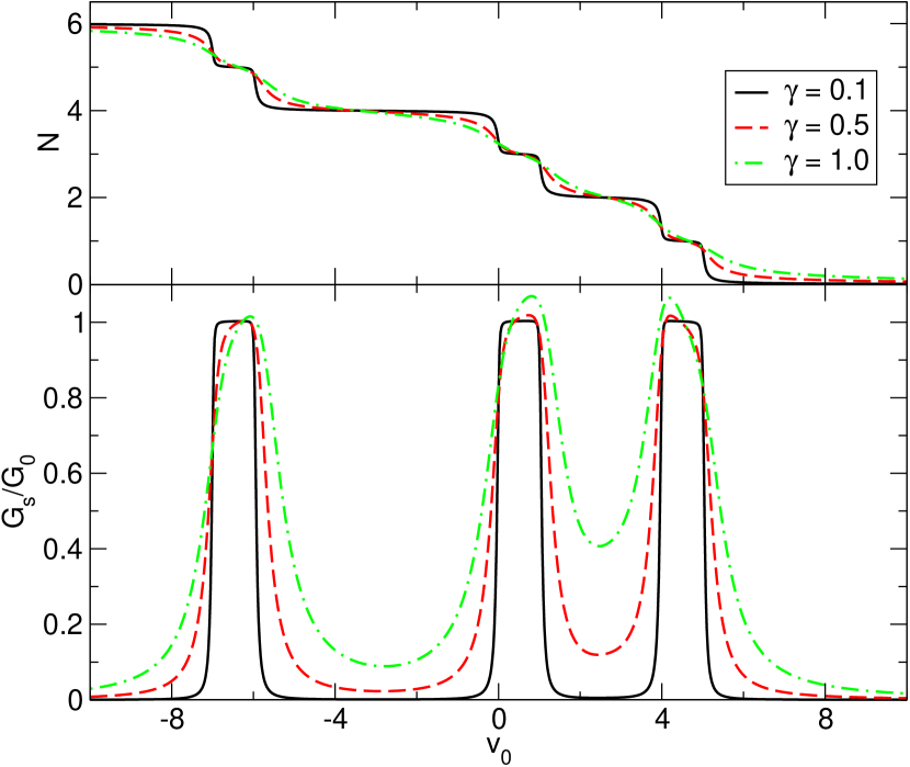
Figure 1: Top: Self-consistent solution of Eq. (23) for the total number $N$ of electrons in the quantum dot. Bottom: KS conductance $G_{s}$ at zero bias, Eq. (25), in units of the quantum of conductance $G_{0}=1/\pi$. Both $N$ and $G_{s}$ are studied as function of the gate voltage $v_{0}$ for three different values of $\gamma=0.1,\;0.5,\;1.0$.

Our first example is a three-level quantum dot with each level twice degenerate due to spin. The single-particle energies are (in arbitrary units) $\epsilon_{l=i\sigma}=\epsilon_{i}^{0}+v_{0}$ with $v_{0}$ the gate voltage, $\epsilon_{1}^{0}=-5$, $\epsilon_{2}^{0}=-3$ and $\epsilon_{3}^{0}=2$, the charging energy $E_{C}=1$, and the broadening matrices $\Gamma_{\alpha}$ are diagonal with diagonal entries equal to $\gamma/2$. We take $\mu=0$ and work at temperature $T=0.001\ll\gamma$, so that the thermal broadening can be discarded and Eq. (18) is a good approximation for $v_{\rm Hxc}$. Since the broadening is the same for all levels we choose the smearing parameter $W(l)=0.16\gamma/E_{C}$ independent of $l$. In Fig. 1 (top) we show the self-consistent solution of Eq. (23) versus gate voltage $v_{0}$ for three different values of $\gamma=0.1,\;0.5,\;1.0$. The discontinuity in $v_{\rm Hxc}$ is crucial to pin the levels to the chemical potential and hence to give rise to the Coulomb blockade ladder. For $v_{0}>5$ the quantum dot is empty since all levels are above $\mu$. For $v_{0}=5$ one electron enters the dot and sits on the first energy level. Due to the fact that the addition of a second electron costs a charging energy $E_{C}=1$ it is not until $v_{0}$ lowers to 4 that a second electron enters. At this point the quantum dot is in a spin singlet with two electrons occuping the first level. The presence of two electrons shifts the unoccupied levels to $\epsilon_{i\sigma}+v_{\rm Hxc}[2]=\epsilon_{i\sigma}+2E_{C}$. Therefore for a third electron to enter the dot $v_{0}$ has to lower to $v_{0}=-\epsilon_{2}^{0}-2E_{C}=3-2=1$. These energetic considerations explain the curve $N$ versus $v_{0}$ from $N=0$, when the quantum dot is empty, to $N=6$, when the quantum dot is totally filled. The message to take home is that the plateaus of the $N$-$v$ curve have length $E_{C}$ if the number of electrons is odd and $E_{C}+\epsilon^{0}_{i+1}-\epsilon^{0}_{i}$ if the number of electrons is even.

Once $N=N(v_{0})$ is known we can proceed with the calculation of the conductance. In Fig. 1 (bottom) we show the zero bias KS conductance of Eq. (25). Interestingly $G_{s}$ exhibits a plateau whenever $N$ is odd, and this behavior is the same as that of the true conductance [45, 46, 47]. The plateau is indeed a consequence of the fact that at low temperatures the true spectral function exhibits a sharp Kondo peak at the chemical potential. The results of Fig. 1 constitute a generalization to multiple levels of the findings in Refs.  [15, 16, 17] and can be explained using the Friedel sum rule [48, 49, 50]. We can conclude that the NEGF-DFT approach, even though based on an adiabatic approximation, is capable to capture strong correlation effects provided that the exact (discontinuous) Hartree-xc potential is used.

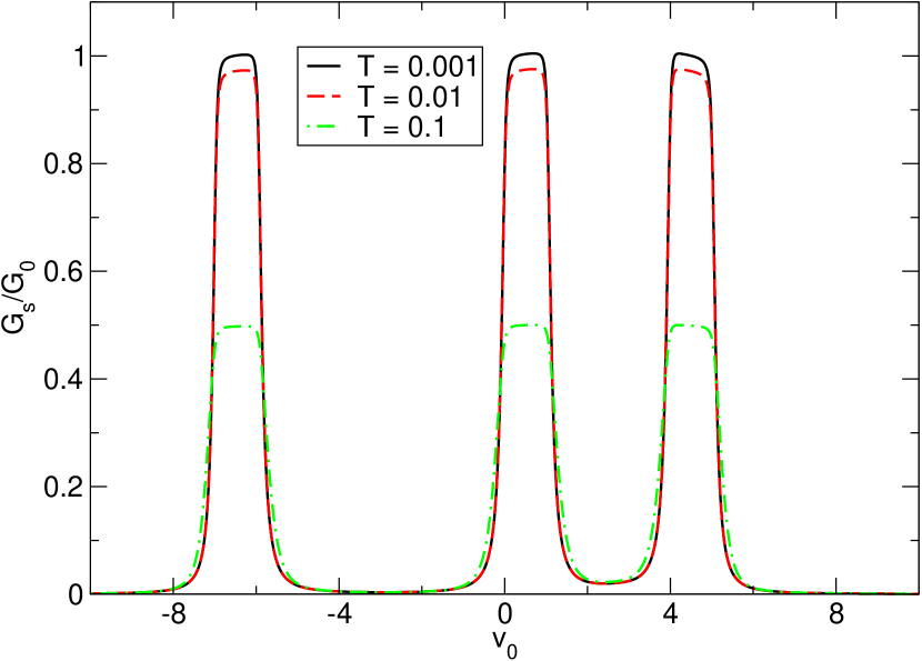
Figure 2: KS conductance $G_{s}$ at zero bias, Eq. (25), in units of the quantum of conductance $G_{0}=1/\pi$ versus the gate voltage $v_{0}$ for $\gamma=0.2$ and three different values of the temperature $T=0.001,\;0.01,\;0.1$.

Unfortunately the agreement between the KS conductance and the true conductance deteriorates with increasing temperature. In Fig. 2 we display $G_{s}$ versus gate voltage for $\gamma=0.2$ and three different values of the temperature $T=0.001,\;0.01,\;0.1$. For temperatures $T$ larger than the Kondo temperature $T_{K}\leq\sqrt{2E_{C}\gamma}\;e^{-\pi E_{C}/8\gamma}\simeq 0.089$ the middle part of the plateau should be suppressed leaving two Coulomb blockade peaks [51, 52]. Instead we see that the entire plateau is suppressed and there is no signature of the Coulomb blockade peaks. As discussed at the end of Section 2, the DFT Hartree-xc potential is weakly dependent on temperature for $T$ smaller than the level broadenings, and therefore our approximation is accurate in this temperature range. Thus, we infer that at finite temperature the adiabatic approximation (which, we recall, is an intrinsic feature of the NEGF+DFT approach) is not able to reproduce the true conductance in the Coulomb blockade regime. In this temperature range the dynamical xc correction of TDDFT is essential [15]. This correction involves the TDDFT kernel with coordinates deep inside the leads [15] and, therefore, is rather difficult to estimate. In fact, the Coulomb blockade regime has remained out of reach until very recently. In Ref. [21] we solved the problem and provided a comprehensive (TD)DFT picture of the Coulomb blockade regime without breaking the spin symmetry.

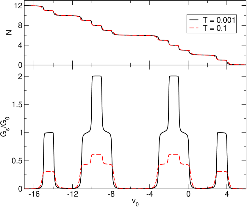
Figure 3: Top: Self-consistent solution of Eq. (23) for the total number $N$ of electrons in the quantum dot. Bottom: KS conductance $G_{s}$ at zero bias, Eq. (25), in units of the quantum of conductance $G_{0}=1/\pi$. Both $N$ and $G_{s}$ are studied as function of the gate voltage $v_{0}$ for two different values of temperature $T=0.001,\;0.1$.

The inadequacy of the NEGF+DFT approach at finite temperature was somehow expected since the relation [48] between the phase-shift (hence the conductance) and the density does not hold any longer. Independently of temperature, no such relation exists for quantum dots with degenerate levels unless the broadening matrices are diagonal. In these cases we expect that at sufficiently low temperature the KS conductance is again in qualitative good agreement with the true conductance.

Let us consider a six-level quantum dot with single-particle energies $\epsilon_{l=i\sigma}=\epsilon_{i}^{0}+v_{0}$ with $v_{0}$ the gate voltage and $\epsilon_{1}^{0}=-4$, $\epsilon_{2}^{0}=\epsilon_{3}^{0}=-2$, $\epsilon_{4}^{0}=\epsilon_{5}^{0}=2$, $\epsilon_{6}^{0}=4$. As in the previous example each level is two-fold degenerate due to spin. We take the charging energy $E_{C}=1$, the broadening matrices diagonal, $[\Gamma_{\alpha}]_{i\sigma,j\sigma^{\prime}}=\delta_{ij}\delta_{\sigma\sigma^{\prime}}\gamma/2$, with $\gamma=0.1$, and hence the smearing parameter $W(l)=0.16\gamma/E_{C}$ independent of $l$. The chemical potential is set to $\mu=0$. In Fig. 3 we show the number of electrons $N$ (top) and KS conductance $G_{s}$ (bottom) versus gate voltage $v_{0}$ for two different temperatures $T=0.001,\;0.1$. According to our parameters when $v_{0}\gtrsim 0$ we have $\epsilon_{2}^{0}+v_{0}+v_{\rm Hxc}[2]=-2+v_{0}+2E_{C}\gtrsim 0$ and therefore the dot has two electrons occupying the lowest energy level. For $v_{0}\lesssim 0$ a third electron enters the dot. At this stage the levels $\epsilon^{0}_{2,3}+v_{0}+v_{\rm Hxc}[3]$ are very close to $\mu$ but not exactly pinned to $\mu$ since the occupancy is $1/2$ for each of them. The KS conductance is the sum of the noninteracting conductances of two single-level models with occupancy $1/2$ since the $\Gamma_{\alpha}$ are diagonal. For occupancy $1/2$ the single-level conductance is $G_{0}/2$ and hence $G_{s}=2G_{0}/2=G_{0}$, in agreement with Fig. 3. Suppose now to lower $v_{0}$ further until the value $v_{0}\simeq-E_{C}$, when a fourth electron enters the dot. With four electrons the levels $\epsilon^{0}_{2,3}+v_{0}+v_{\rm Hxc}[4]$ are exactly pinned to $\mu$ since the occupancy is $1$ for each of them. For occupancy 1 the single-level conductance is $G_{0}$ and hence $G_{s}=2G_{0}$. This explains the second plateau at $2G_{0}$ for $-1\lesssim v_{0}\lesssim 0$. With similar arguments we can understand all remaining plateaus. This behavior of $G_{s}$ is qualitatively similar to that of the true conductance [47, 53]. The effect of increasing temperature on $G_{s}$ is to lower the plateaus. The true conductance, instead, develops distinct Coulomb blockade peaks [47, 53]. We conclude that the NEGF-DFT approach accounts for degeneracy effects reasonably well (for diagonal $\Gamma$-matrices) whereas it needs to be considerably revised in order to include finite temperature effects (Coulomb blockade regime) [21].

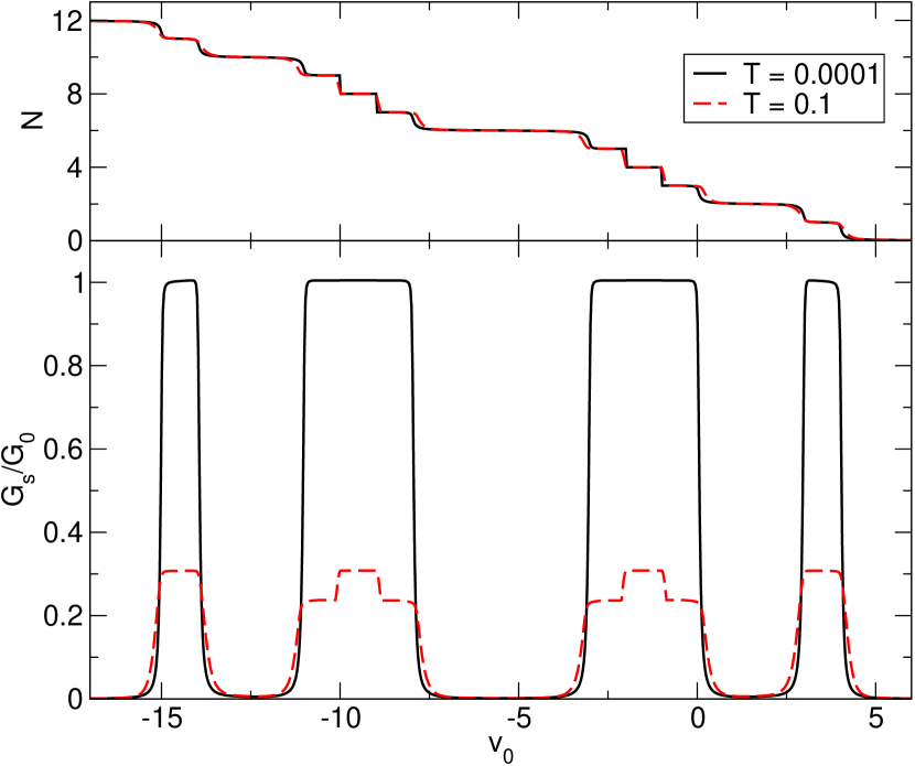
Figure 4: Same system as in Fig. 3 except for $[\Gamma_{\alpha}]_{3\sigma,3\sigma}=[\Gamma_{\alpha}]_{5\sigma,5\sigma}=0$. The self-consistent solution for $N$ (top) has been obtained by modifying the Hartree-xc potential as described in the main text.

We also studied a variant of the previous six-levels quantum dot in which one of the degenerate levels in each multiplet, say $\epsilon_{3\sigma}$ and $\epsilon_{5\sigma}$, do not hybridize with the leads and hence $[\Gamma_{\alpha}]_{3\sigma,3\sigma}=[\Gamma_{\alpha}]_{5\sigma,5\sigma}=0$. Consider the dot with two electrons in the lowest energy level $\epsilon_{1\sigma}$. By lowering $v_{0}$ a third electron enters the dot. Unlike the previous case this electron does not equally distribute between levels $\epsilon_{2\sigma}$ and $\epsilon_{3\sigma}$ but occupies only level $\epsilon_{2\sigma}$. Indeed $\epsilon_{2\sigma}$ hybridizes with the leads and hence it gets half populated when $\epsilon_{2\sigma}=0+\delta$ with $\delta$ a small positive constant. Since any $\delta>0$ is larger than the broadening of level $\epsilon_{3\sigma}$, this level remains empty. By lowering $v_{0}$ further we eventually start occupying level $\epsilon_{3\sigma}$. The population of this level occurs very rapidly since it is not coupled to the leads. From these considerations we see that the form of $v_{\rm Hxc}$ in Eq. (17) needs to be modified. For instance, according to the previous argument, for $2<N<3$ the smearing parameter $W(3)$ is finite but for $3<N<4$ the same smearing parameter vanishes. Therefore we introduce $N$-dependent smearing parameters $W(l,N)$ in Eq. (17) according to

$$W(3,N) = \theta(3-N)W$$

$$W(4,N) = 0$$

$$W(5,N) = \theta(N-5)W$$

$$W(7,N) = \theta(7-N)W$$

$$W(8,N) = 0$$

$$W(9,N) = \theta(N-9)W$$

and $W(1)=W(2)=W(6)=W(10)=W(11)=W(12)=W=0.16\gamma/E_{C}$. The self-consistent solution of Eq. (23) is shown in Fig. 4 (top). The modified Hartree-xc potential correctly reproduces the trend of $N$ versus $v_{0}$ deduced from physical arguments. The transitions $0\to 1\to 2\to 3$ electrons are smooth whereas the transitions $3\to 4\to 5$ are sharp. The same behavior is observed for the other pair of degenerate levels. The corresponding KS conductance is displayed in Fig. 4 (bottom). The main difference with the previous case is that the plateau at $2G_{0}$ lowers to $G_{0}$. This can be understood as follows. With 3 electrons in the quantum dot the level $\epsilon_{2\sigma}$ is half filled while level $\epsilon_{3\sigma}$ is empty. Since level $\epsilon_{2\sigma}$ is coupled to the leads the conductance is $G_{s}=G_{0}$. With 4 and 5 electrons level $\epsilon_{2\sigma}$ remains half filled and level $\epsilon_{3\sigma}$ is half-filled and totally filled respectively. This level, however, is not coupled to the leads and hence does not contribute to the conductance which remains equal to $G_{0}$. With similar energetic considerations we can explain all remaining plateaus. With increasing temperature the thermal broadening of the Fermi function allows for a slight distribution of electrons. When a third electron enters the dot we have little occupancy of level $\epsilon_{3\sigma}$ as well. Thus level $\epsilon_{2\sigma}$ is not exactly half filled and the conductance is lower than that with 4 electrons when level $\epsilon_{2\sigma}$ is instead half filled.

5 Conclusions and outlooks

We generalized the findings of Ref. [15] to multiple levels, relevant for quantum dots or molecular junctions. At temperatures below the Kondo temperature and for nondegenerate levels the NEGF-DFT approach is very accurate provided that the exact DFT Hartree-xc potential is used. The success of NEGF-DFT has its origin in the fulfillment of the Friedel sum rule. At finite temperature the Friedel sum rule is of no use to relate the conductance to the density and we indeed find that the KS and true conductances can differ quite substantially. Another situation for which, in general, we cannot use the Friedel sum rule is that of degenerate levels. An exception is that of diagonal $\Gamma$ matrices. In this case the NEGF-DFT approach is again exact provided that the exact DFT Hartree-xc potential is employed. For the CIM we constructed an approximation to $v_{\rm Hxc}$ which becomes exact in the limit of weak coupling. Our results for the (KS) conductance are in good qualitative agreement with numerical renormalization group results [47] and many-body results [53]. In all other cases one has to go beyond the NEGF-DFT approach and include dynamical xc corrections in the theory. This can be done either by finding suitable approximations to the TDDFT kernel and then solving the linear response equations or by including memory effects in the TDDFT Hartree-xc potential [54, 55, 56, 57, 58] and then performing time propagations. There has been considerable progress in the implementation of ab initio propagation schemes for open systems [59, 60, 61, 62, 63, 43, 44, 64, 65, 66] but, at present, the results are limited to adiabatic Hartree-xc potentials. The development of propagation algorithms for open systems with nonadiabatic Hartree-xc potentials represents one of the future challenges in quantum transport.

S.K. acknowledges funding by the “Grupos Consolidados UPV/EHU del Gobierno Vasco” (IT-578-13). G.S. acknowledges funding by MIUR FIRB grant No. RBFR12SW0J. We also acknowledge financial support through travel grants (Psi-K2 4665 and 3962 (G.S.), and Psi-K2 5332 (S.K.)) of the European Science Foundation (ESF).

References

- [1] N. A. Lima, L. N. Oliveira and K. Capelle, Europhys. Lett. 60, 601 (2002).
- [2] N. A. Lima, M. F. Silva, L. N. Oliveira and K. Capelle, Phys. Rev. Lett. 90, 146402 (2003).
- [3] P. Mori-Sanchez, A. J. Cohen and W. Yang, Phys. Rev. Lett. 102, 066403 (2009).
- [4] F. Malet and P. Gori-Giorgi, Phys. Rev. Lett. 109, 246402 (2012).
- [5] F. Malet, A. Mirtschink, J. C. Cremon, S. M. Reimann and P. Gori-Giorgi, Phys. Rev. B 87, 115146 (2013).
- [6] Gao Xianlong, A-Hai Chen, I. V. Tokatly and S. Kurth, Phys. Rev. B 86, 235139 (2012).
- [7] J. Lorenzana, Z.-J. Ying and V. Brosco, Phys. Rev. B 86, 075131 (2012).
- [8] E. Kraisler and L. Kronik, Phys. Rev. Lett. 110, 126403 (2013).
- [9] C. Verdozzi, Phys. Rev. Lett. 101, 166401 (2008).
- [10] S. Kurth, G. Stefanucci, E. Khosravi, C. Verdozzi and E. K. U. Gross, Phys. Rev. Lett. 104, 236801 (2010).
- [11] D. Hofmann and S. Kümmel, Phys. Rev. B 86, 201109 (2012).
- [12] P. Elliott, J. I. Fuks, A. Rubio and N. T. Maitra, Phys. Rev. Lett. 109, 266404 (2012).
- [13] S. E. B. Nielsen, M. Ruggenthaler and R. van Leeuwen, EPL 101, 33001 (2013).
- [14] J. P. Perdew, R. G. Parr, M. Levy, and J. L. Balduz, Phys. Rev. Lett. 49, 1691 (982).
- [15] G. Stefanucci and S. Kurth, Phys. Rev. Lett. 107, 216401 (2011).
- [16] J. P. Bergfield, Z.-F. Liu and K. Burke, Phys. Rev. Lett. 108, 066801 (2012).
- [17] P. Tröster, P Schmitteckert and F. Evers, Phys. Rev. B 85, 115409 (2012).
- [18] L. P. Kouwenhoven, D. G. Austing and S. Tarucha, Rep. Prog. Phys. 64, 701 (2001).
- [19] N. D. Mermin, Phys. Rev. 137, A1441 (1965).
- [20] Y. Oreg, K. Byczuk and B. I. Halperin, Phys. Rev. Lett. 85, 365 (2000).
- [21] S. Kurth and G. Stefanucci, Phys. Rev. Lett. 111, 030601 (2013).
- [22] F. Evers and P. Schmitteckert, Phys. Chem. Chem. Phys. 13, 14 417 (2011).
- [23] P. B. Wiegmann and A. M. Tsvelick, J. Phys. C: Solid State Phys. 16, 2281 (1983).
- [24] E. Perfetto and G. Stefanucci, Phys Rev B 86, 081409 (2012).
- [25] R. Landauer, IBM J. Res. Dev. 1, 233 (1957).
- [26] Y. Meir and N. S. Wingreen, Phys. Rev. Lett. 68, 2512 (1992).
- [27] A.-P. Jauho, N. S. Wingreen and Y. Meir, Phys. Rev. B 50, 5528 (1994).
- [28] N. D. Lang, Phys. Rev. B 52, 5335 (1995).
- [29] N. D. Lang and P. Avouris, Phys. Rev. Lett. 81, 3515 (1998).
- [30] J. Taylor, H. Guo and J. Wang, Phys. Rev. B 63, 121104 (2001).
- [31] J. Taylor, H. Guo and J. Wang, Phys. Rev. B 63, 245407 (2001).
- [32] M. Brandbyge, J.-L. Mozos, P. Ordejón, J. Taylor and K. Stokbro, Phys. Rev. B 65, 165401 (2002).
- [33] E. Runge and E. K. U. Gross, Phys. Rev. Lett. 52, 997 (1984).
- [34] G. Stefanucci and C.-O. Almbladh, Phys. Rev. B 69, 195318 (2004).
- [35] G. Stefanucci and C.-O. Almbladh, Europhys. Lett. 67, 14 (2004).
- [36] G. Stefanucci, Phys. Rev. B 75, 195115 (2007).
- [37] F. Evers, F. Weigend and M. Koentopp, Phys. Rev. B 69, 235411 (2004).
- [38] N. Sai, M. Zwolak, G. Vignale and M. Di Ventra, Phys. Rev. Lett. 94, 186810 (2005).
- [39] M. Koentopp, K. Burke and F. Evers, Phys. Rev. B 73, 121403 (2006).
- [40] G. Stefanucci, S. Kurth, E. K. U. Gross and A. Rubio, Time-dependent transport phenomena, in: J. M. Seminario (Ed.), Molecular and nano electronics: analysis, design and simulation, Vol. 17 of Elsevier Series on Theoretical and Computational Chemistry, Elsevier, 2007, p. 247.
- [41] M. Thiele, E. K. U. Gross and S. Kümmel, Phys. Rev. Lett. 100, 153004 (2008).
- [42] M. Thiele and S. Kümmel, Phys. Rev. A 79, 052503 (2009).
- [43] C. Yam, X. Zheng, G. H. Chen, Y. Wang, T. Frauenheim and T. A. Niehaus, Phys. Rev. B 83, 245448 (2011).
- [44] Y. Wang, C. Yam, T. Frauenheim, G. H. Chen and T. A. Niehaus, Chem. Phys. 391, 69 (2011).
- [45] A. Oguri, Y. Nisikawa and A. C. Hewson, J. Phys. Soc. Jpn. 74, 2554 (2005).
- [46] Y. Nisikawa and A. Oguri, Phys. Rev. B 73, 125108 (2006).
- [47] W. Izumida, O. Sakai and Y. Shimizu J. Phys. Soc. Jpn. 67, 2444 (1998).
- [48] D. C. Langreth, Phys. Rev. 150, 516 (1966).
- [49] H. Mera, K. Kaasbjerg, Y. M. Niquet, and G. Stefanucci, Phys. Rev. B 81, 035110 (2010).
- [50] H. Mera and Y. M. Niquet, Phys. Rev. Lett. 105, 216408 (2010).
- [51] W. Izumida and O. Sakai, J. Phys. Soc. Jpn. 74, 103 (2005).
- [52] T. A. Costi, Phys. Rev. Lett. 85, 1504 (2000).
- [53] A. Levy Yeyati, F. Flores and A. Martìn-Rodero, Phys. Rev. Lett. 83, 600 (1999).
- [54] J. F. Dobson, M. J. Bünner and E. K. U. Gross, Phys. Rev. Lett. 79, 1905 (1997).
- [55] N. T. Maitra, K. Burke and C. Woodward, Phys. Rev. Lett. 89, 023002 (2002)
- [56] U. von Barth, N. E. Dahlen, R. van Leeuwen and G. Stefanucci, Phys. Rev. B 72, 235109 (2005).
- [57] I. V. Tokatly, Phys. Rev. B 75, 125105 (2007).
- [58] N. T. Maitra, Lectures Notes in Physics 837, 167 (2012).
- [59] R. Baer, T. Seideman, S. Ilani, and D. Neuhauser, J. Chem. Phys. 120, 3387 (2004).
- [60] S. Kurth, G. Stefanucci, C.-O. Almbladh, A. Rubio and E. K. U. Gross, Phys. Rev. B 72, 035308 (2005).
- [61] X. Zheng, F. Wang, C. Y. Yam, Y. Mo and G. H. Chen, Phys. Rev. B 75, 195127 (2007).
- [62] N. Sai, N. Bushong, R. Hatcher, and M. Di Ventra, Phys. Rev. B 75, 115410 (2007).
- [63] G. Stefanucci, E. Perfetto and M. Cini, Phys. Rev. B 81, 115446 (2010).
- [64] L. Zhang, B. Wang and Jian Wang, Phys. Rev. B 86, 165431 (2012).
- [65] L. Zhang, Y. Xing and J. Wang, Phys. Rev. B 86, 155438 (2012).
- [66] Y. Zhang, S. Chen and G. H. Chen, Phys. Rev. B 87, 085110 (2013).