On the necessary conditions for bursts of convection within the rapidly rotating cylindrical annulus

Abstract

Zonal flows are often found in rotating convective systems. Not only are these jet-flows driven by the convection, they can also have a profound effect on the nature of the convection. In this work the cylindrical annulus geometry is exploited in order to perform nonlinear simulations seeking to produce strong zonal flows and multiple jets. The parameter regime is extended to Prandtl numbers that are not unity. Multiple jets are found to be spaced according to a Rhines scaling based on the zonal flow speed, not the convective velocity speed. Under certain conditions the nonlinear convection appears in quasi-periodic bursts. A mean field stability analysis is performed around a basic state containing both the zonal flow and the mean temperature gradient found from the nonlinear simulations. The convective growth rates are found to fluctuate with both of these mean quantities suggesting that both are necessary in order for the bursting phenomenon to occur.

I Introduction

An interest in zonal flows originates from a desire to better explain various phenomena observed in geophysical and astrophysical bodies. These large azimuthal flows found in the atmospheres of the gas giants as well as planetary cores are thought to be driven by the interaction of convection and rotation. Jupiter, for example, has a clear banded structure of jets, made up of alternating prograde and retrograde zonal flows Limaye (1986); Porco et al. (2003). This pattern extends over the whole planet and the zonal flows are considerably stronger than the radial convection. Although the convection in both the deep Jovian atmosphere and the Earth’s outer core will be affected by their respective magnetic fields, an understanding of the non-magnetic problem can provide insight to the physical structures observed. The depth to which the zonal flows extend in Jupiter’s atmosphere is not known, though there is evidence to suggest that flows are considerably weaker in the core compared with the surface Starchenko and Jones (2002). BusseBusse (1976) suggested a model for convection in the Jovian atmosphere where zonal flows are not confined to the surface. The difficulties in modeling the interiors of the major planets has been discussed by YanoYano (1998).

The linear theory of convection in spheres and spherical shells has now been comprehensively investigated. RobertsRoberts (1968) and BusseBusse (1970) derived some of the basic principles and the rapid rotation limit was discussed by Jones et al.Jones et al. (2000) and Dormy et al.Dormy et al. (2004). However, performing three-dimensional nonlinear simulations in spherical geometry can be computationally expensive. Quasi-geostrophic models (Busse, 1970; Gillet and Jones, 2006; Rotvig, 2007) assume that the rapid rotation leads to columnar structures with little $z$-dependence, leading to two-dimensional models. The Busse annulus Busse (1970); Busse and Or (1986); Busse (1986); Or and Busse (1987); Schnaubelt and Busse (1992) is one such quasi-geostrophic model. It replicates several key aspects of convection in spherical geometry; for example, convection occurs in the form of tall thin columns which onset as thermal Rossby waves (Busse and Or, 1986). Of particular relevance is the nonlinear model’s ability to develop large zonal flows which may have a multiple jet structure Jones et al. (2003).

Zonal flows have been found both in laboratory experiments Busse and Carrigan (1976); Manneville and Olson (1996); Aubert et al. (2001) and nonlinear simulations in the annulus (Brummell and Hart, 1993; Jones et al., 2003; Rotvig and Jones, 2006) and in the more physically realistic spherical shell geometry Gilman (1977, 1978a, 1978b); Zhang (1992); Tilgner and Busse (1997); Grote and Busse (2001); Christensen (2001, 2002); Busse (2002); Heimpel et al. (2005). Simulations of rotating convection in spherical shells were undertaken by GilmanGilman (1977, 1978a, 1978b) and ZhangZhang (1992) which produced zonal flows. More recent simulations Tilgner and Busse (1997); Aurnou and Olson (2001); Christensen (2001, 2002); Busse (2002); Heimpel et al. (2005); Heimpel and Aurnou (2007) have produced strong zonal flows, driven by the Reynolds stresses, with Rossby numbers of the correct order of magnitude. Interestingly, both steady and oscillatory solutions were found resulting in the discovery of a ‘bursting phenomenon’ Grote and Busse (2001). The bursting phenomenon, investigated within the annulus model by Rotvig and JonesRotvig and Jones (2006), and in a quasi-geostrophic model taking account of the curvature of the boundaries by Morin and DormyMorin and Dormy (2004) refers to the observation that convection can occur as short-lived bursts rather than the system evolving into a quasi-steady equilibrium. These bursts of convection are currently thought to be a result of a competition between the zonal flow and the convection. The convection drives up the zonal flow strongly, but this zonal flow eventually disrupts the convection, which then cannot sustain the zonal flow. The zonal flow dies away, allowing convection to occur again, and repeat the cycle.

The three-dimensional simulations discussed above often do not produce a multiple jet structure of the zonal flow. The reason is that to get multiple jets very large rotation rates (very low Ekman numbers) are required Jones et al. (2003). Due to numerical difficulties the fully three-dimensional models have often been unable to achieve the rotation rate required, though in some exceptionally high-resolution three-dimensional simulations multiple jets have been found Heimpel et al. (2005); Heimpel and Aurnou (2007).

One of the attractions of the annulus model, as a simplified model for convection in the Jovian atmosphere, lies in its ability to produce both multiple jets and the bursts of convection. However, these properties are dependent on the boundary conditions. In general, stronger zonal flows and bursting are produced when stress-free top and bottom boundaries are imposed Gilman (1978b); Brummell and Hart (1993); Christensen (2001) whereas no-slip boundaries are able to generate a multiple jet structure Jones et al. (2003). Similar results were found in the quasi-geostrophic model by Morin and DormyMorin and Dormy (2006). The work of Rotvig and JonesRotvig and Jones (2006) shows that multiple jets and bursting appear to be mutually exclusive when the Prandtl number is unity.

The aims of this paper are three-fold. Firstly we wish to extend the simulations performed by Rotvig and JonesRotvig and Jones (2006) to parameter regimes where the Prandtl number is not unity. Secondly, we wish to check the consistency of our results with the Rhines scaling theory Rhines (1975). Thirdly, we wish to investigate what role the nonlinear interaction of temperature fluctuations have in the generation of bursts of convection since a mean temperature gradient is known to evolve when performing simulations. Note that the zonal flow in this work is generated by the nonlinear Reynolds stress, rather than by a thermal wind, for which the dynamics is rather different Teed et al. (2010). To aid the reader we summarize in table 1 several quantities that appear in the article.

Quantities	Section	Definition	Explanation
$\bar{U}(y)$	III	$\langle u_{x}\rangle_{x}$	$x$-averaged velocity (zonal flow) from nonlinear simulations
$\bar{\theta}(y)$	III	$\langle\theta\rangle_{x}$	$x$-averaged (mean) temperature from nonlinear simulations
$\bar{\theta}^{\prime}(y)$	III	$\langle\theta^{\prime}\rangle_{x}$	$x$-averaged (mean) temperature gradient from nonlinear simulations
$\bar{U}_{\text{max}}$	III.4	$\max(\bar{U}(y))$	Maximum value that $\bar{U}(y)$ takes in the domain
$\bar{U}_{\text{min}}$	III.4	$\min(\bar{U}(y))$	Minimum value that $\bar{U}(y)$ takes in the domain
$\bar{\theta}^{\prime}_{\text{max}}$	III.4	$\max(\bar{\theta}^{\prime}(y))$	Maximum value that $\bar{\theta}^{\prime}(y)$ takes in the domain
$\bar{\theta}^{\prime}_{\text{min}}$	III.4	$\min(\bar{\theta}^{\prime}(y))$	Minimum value that $\bar{\theta}^{\prime}(y)$ takes in the domain
$U_{0}(y)$	IV		Zonal flow included in the basic state of the linear theory
$G_{0}(y)$	IV		Mean temperature included in the basic state of the linear theory

Table 1: Definition and explanation of quantities used in this article along with the section for which they first appear.

II Mathematical setup

We consider a fluid filled cylindrical annulus with inclined bounding surfaces for the top and bottom lids, see figure 1. The mean radius of the annulus is $r_{0}$, the gap between the two cylinders, referred to as the width, is $D$, and the height of the annulus at the outer cylindrical wall is $L$. The annulus rotates about the axial direction with angular velocity $\Omega$ and a temperature difference of $\Delta T$ is maintained between the two walls such that the outer and inner walls are at temperatures $T=0$ and $T=\Delta T$ respectively. We also take the gravity force to be acting radially inward and the annular end walls make an angle $\chi$ to the horizontal.

The natural choice of coordinate system for the annulus model would be cylindrical polar coordinates: $(r,\phi,z)$. However, by making the small-gap approximation of $D/r_{0}\ll 1$, the curvature terms of cylindrical polars can be neglected and Cartesian coordinates can be used. The azimuthal coordinate is $x$ and it increases eastwardly (acting like $\phi$) and $0\leq y\leq D$ is the radial coordinate (acting like $-r$). The axial coordinate, $z$, remains unchanged from cylindrical polars and ranges from $-L/2$ to $L/2$. Consequently, gravity acts in the positive $y$-direction and the direction of rotation is in the $z$-direction so that $\mathbf{g}=g\mathbf{\hat{y}}$ and $\mathbf{\Omega}=\Omega\mathbf{\hat{z}}$. The no penetration condition at the sloped end walls of the annulus is dependent on the inclination, $\chi$, so that

$$\cos(\chi)u_{z}\mp\sin(\chi)u_{y}\mp U_{E}=0\quad\textrm{on}\quad z\pm L/2.$$ (1)

Here $U_{E}$ is an Ekman suction or ‘bottom friction’ term derived using the theory described by GreenspanGreenspan (1968). The purpose of the term is to replicate the effects of the Ekman boundary layer that arises when rigid boundaries are implemented. Hence $U_{E}$ is present only when no-slip rather than stress-free boundaries are required.

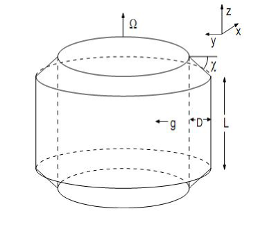
Figure 1: Diagram depicting the physical setup of the Busse annulus; reproduced from Abdulrahman et al.Abdulrahman et al. (2000).

The linear theory of the annulus model was originally discussed and solved by BusseBusse (1970); Busse and Or (1986). We use the $z$-component of the vorticity equation, which is

$$\frac{\partial\zeta}{\partial t}+\mathbf{u}\cdot\nabla\zeta-2\Omega\mathbf{\hat{z}}\cdot\frac{\partial\mathbf{u}}{\partial z}=-g\alpha\frac{\partial T}{\partial x}+\nu\nabla^{2}\zeta,$$ (2)

where $\zeta$ is the $z$-component of the vorticity. Here we have neglected the $(\boldsymbol{\zeta}\cdot\nabla)\mathbf{u}$ term that usually appears in the vorticity equation since we are interested in the small Rossby number limit of rapid rotation where the planetary vorticity $2{\Omega}$ dominates over the fluid vorticity $\zeta$. This is the standard practice in the annulus model as well as other quasi-geostrophic models Gillet and Jones (2006). In the annulus model the term is of order $\chi$, which is taken to be much smaller than unity, while the other nonlinear terms are of order 1 as discussed by Busse and OrBusse and Or (1986).

We perturb around the basic state to acquire a similar set of equations to those of Busse, including nonlinear terms. We write $T=T_{0}+\theta$, where $T_{0}=y\Delta T/d$ is the conduction state profile, and assume that $\chi\ll 1$. Hence the boundaries are nearly flat, the flow is nearly geostrophic and the $z$-component of the velocity is small compared with the horizontal components. This allows us to make the ansatz

$$\mathbf{u}=-\nabla\times\psi(x,y)\mathbf{\hat{z}}+u_{z}\mathbf{\hat{z}},$$ (3)

where the vertical velocity, $u_{z}$, is a small ageostrophic part of the flow of order $\chi$. We substitute the perturbed forms of the the fields into equation (2) as well as the relevant heat equation and integrate over $z$ applying the conditions of equation (1) at the sloped boundaries. We also non-dimensionalize using the length scale $D$, the viscous timescale $D^{2}/\nu$ and the temperature scale $\nu\Delta T/\kappa$. This gives

$$\frac{\partial\nabla^{2}\psi}{\partial t}+\frac{\partial(\psi,\nabla^{2}\psi)}{\partial(x,y)}-\beta\frac{\partial\psi}{\partial x}=-Ra\frac{\partial\theta}{\partial x}-C|\beta|^{1/2}\nabla^{2}\psi+\nabla^{4}\psi,$$ (4)

$$Pr\left(\frac{\partial\theta}{\partial t}+\frac{\partial(\psi,\theta)}{\partial(x,y)}\right)=-\frac{\partial\psi}{\partial x}+\nabla^{2}\theta,$$ (5)

where the Jacobian, $\partial(A,B)/\partial(x,y)=(\partial_{x}A)(\partial_{y}B)-(\partial_{x}B)(\partial_{y}A)$ for some functions $A$ and $B$, has been introduced. We have eliminated the vorticity by noting that $\zeta=\nabla^{2}\psi$. The beta parameter, $\beta$, Prandtl number, $Pr$, and Rayleigh number, $Ra$, are defined as

$$\beta=\frac{4\chi\Omega D^{3}}{\nu L},\qquad Pr=\frac{\nu}{\kappa},\qquad Ra=\frac{g\alpha\Delta TD^{3}}{\nu\kappa}.$$ (6)

In the annulus model the beta parameter effectively acts as an inverse Ekman number and therefore in the limit of rapid rotation we expect $\beta$ to be large. The small angle assumption has allowed us to write $U_{E}=-D^{3/2}\zeta(\chi/\beta L)^{1/2}$ for the Ekman suction Jones (2007) and the term (in equation (4)) resulting from this bottom friction contains the parameter $C=(D/L\chi)^{1/2}$. Since the bottom friction is a phenomenon associated only with rigid boundaries we explicitly set $C=0$ when implementing stress-free boundary conditions.

Since we have used the boundary conditions on the sloped end walls in order to integrate $z$ out of the problem, the only boundaries left to consider are those at the inner and outer walls of the cylinders. Equations (4 - 5) form a sixth order system of equations and thus we require six boundary conditions at $y=0$ and $y=1$. As well as there being no penetration we also demand these boundaries to be stress-free and have constant surface temperature so that

$$u_{y}=0\Rightarrow\frac{\partial\psi}{\partial x}=0,\qquad\frac{\partial u_{x}}{\partial y}=0\Rightarrow\frac{\partial^{2}\psi}{\partial y^{2}}=0,\qquad\theta=0,$$ (7)

at $y=0$ and $y=1$.

III Nonlinear results

We perform nonlinear simulations of the equations (4-5). The system has four input parameters: $Pr,\beta,Ra$ and $C$. We integrate these nonlinear equations forward in time using a pseudo-spectral collocation method Boyd (2001). We expand $\psi$ and $\theta$ using a Fourier and sine expansion in the $x$ and $y$-directions respectively. We therefore write

$$\psi(x,y,t)=\frac{1}{2}\sum_{l=-N_{x}}^{N_{x}}\sum_{m=1}^{N_{y}-1}\hat{\psi}_{lm}(t)e^{-\mathrm{i}lx(2\pi/L_{x})}\sin(m\pi y),$$ (8)

$$\theta(x,y,t)=\frac{1}{2}\sum_{l=-N_{x}}^{N_{x}}\sum_{m=1}^{N_{y}-1}\hat{\theta}_{lm}(t)e^{-\mathrm{i}lx(2\pi/L_{x})}\sin(m\pi y),$$ (9)

where we note that the choice of a sine expansion implicitly satisfies the boundary conditions of equation (7). Since $\psi$ is real, we have that $\hat{\psi}_{-lm}=\hat{\psi}^{*}_{lm}$, where $*$ denotes complex conjugate.

The simulations are performed by implementing the Crank-Nicolson method to all but the nonlinear terms and a second-order Adams-Bashforth scheme to the nonlinear terms. Hence we use a semi-implicit method with only the nonlinear terms being calculated explicitly. We define ‘mean quantities’ as follows. The zonal flow, $\bar{\mathbf{U}}$, is the $x$-average of the azimuthal component of the velocity, and $\bar{\theta}$ is the mean temperature so

$$\bar{\mathbf{U}}=\bar{U}\mathbf{\hat{x}}=\langle u_{x}\rangle_{x}\mathbf{\hat{x}}=-\frac{\partial\langle\psi\rangle_{x}}{\partial y}\mathbf{\hat{x}},\qquad\textrm{and}\qquad\bar{\theta}=\langle\theta\rangle_{x}.$$ (10)

The $x$-average is defined as $\langle A\rangle_{x}=(1/L_{x})\int_{0}^{L_{x}}A\mathrm{d}x$, for a scalar quantity, $A$. The only contribution to the mean quantities comes from modes with $l=0$ so that

$$\bar{U}=-\frac{1}{2}\sum_{m=1}^{N_{y}-1}m\pi\hat{\psi}_{0m}\cos(m\pi y)\qquad\textrm{and}\qquad\bar{\theta}=\frac{1}{2}\sum_{m=1}^{N_{y}-1}\hat{\theta}_{0m}\sin(m\pi y).$$ (11)

Zonal flow generation is governed byRotvig and Jones (2006)

$$\frac{\partial\bar{U}}{\partial t}=-\frac{\partial}{\partial y}\langle u_{x}u_{y}\rangle_{x}-C|\beta|^{1/2}\bar{U}+\frac{\partial^{2}\bar{U}}{\partial y^{2}}.$$ (12)

We note that zonal flow can be created by the Reynolds force, confirming that $\bar{U}$ is a nonlinear phenomenon, and destroyed by the friction terms. The addition of the bottom friction term is expected therefore to dampen the zonal flow; however, as discussed in section I, we expect it to increase the likelihood of multiple jet solutions arising. Also of interest are the total kinetic energy and the zonal part of the kinetic energy, defined by

$$E_{T}=\frac{1}{L_{x}}\int(\nabla\psi)^{2}\mathrm{d}S=\frac{1}{8}\sum_{l=0}^{N_{x}}\sum_{m=1}^{N_{y}-1}\left(\frac{4\pi^{2}l^{2}}{L_{x}^{2}}+m^{2}\pi^{2}\right)|\hat{\psi}_{lm}|^{2},\qquad\textrm{and}$$ (13)

$$E_{Z}=\frac{1}{L_{x}}\int(\langle\nabla\psi\rangle_{x})^{2}\mathrm{d}S=\frac{1}{8}\sum_{m=1}^{N_{y}-1}m^{2}\pi^{2}|\hat{\psi}_{0m}|^{2},$$ (14)

respectively.

In table 2 we list the runs performed, which lie in the range $0.2\leq Pr\leq 5$ and $10^{3}<\beta<10^{6}$. $L_{x}$ is set at $2\pi$, which is sufficiently large since the structures in the $x$ direction have short wavelengths. In the previous work Jones et al. (2003); Rotvig and Jones (2006) only Prandtl number unity was considered. We perform runs with the Rayleigh number 2.5, 2.75, 5 and 10 times that of the critical Rayleigh number for a given $Pr$ and $\beta$ as indicated in table 2. The rapid rotation approximation Busse and Or (1986) to the critical Rayleigh number for the Busse annulus

$$Ra_{c}=\frac{3\beta^{4/3}Pr^{4/3}}{2^{2/3}(1+Pr)^{4/3}},$$ (15)

is adequate at these high $\beta$.

Run	$Pr$	$\beta$	$C$	$Ra/Ra_{c}$	$\tau$	$m_{*}$	Range of $\bar{U}_{\text{max}}$	Range of $\bar{\theta}^{\prime}_{\text{max}}$	Bursting
I	$1$	$7.07\times 10^{3}$	$0.316$	$2.5$	$13.12$	$2$	$2-37$	$1.2-3.2$	No
II	$1$	$7.07\times 10^{5}$	$0$	$2.5$	$1.65$	$2$	${587-679}$	$0.9-1.9$	Yes
III	$1$	$7.07\times 10^{4}$	$0$	$2.5$	$3.63$	$1$	${319-534}$	$0.2-3.2$	Yes
IV	$1$	$7.07\times 10^{4}$	$0.00316$	$2.5$	$1.23$	$2$	${210-298}$	$0.5-2.5$	Yes
V	$1$	$7.07\times 10^{4}$	$0.316$	$2.5$	$8.08$	$3$	$12-156$	$2.2-4.1$	No
VI	$1$	$7.07\times 10^{5}$	$0.316$	$2.5$	$2.68$	$5$	$401-521$	$2.2-3.3$	No
VII	$1$	$5\times 10^{5}$	$0$	$2.75$	$3.29$	$2$	${834-1176}$	$0.4-3.2$	Yes
VIII	$1$	$5\times 10^{5}$	$0$	$5$	$0.93$	$2$	${2591-4701}$	$1.0-7.7$	Yes
IX	$1$	$5\times 10^{5}$	$0.05$	$2.75$	$1.44$	$3$	$764-921$	$0.85-2.9$	No
X	$1$	$5\times 10^{5}$	$0.5$	$2.75$	$3.38$	$5$	$371-430$	$3.4-5.0$	No
XI	$0.5$	$5\times 10^{5}$	$0$	$2.75$	$2.69$	$2$	$903-1046$	$0.35-1.05$	No
XII	$0.5$	$5\times 10^{5}$	$0$	$5$	$0.25$	$1$	${3993-5489}$	$0.1-6.5$	Yes
XIII	$0.5$	$5\times 10^{5}$	$0.5$	$2.75$	$2.64$	$4$	$372-570$	$1.5-2.5$	No
XIV	$2$	$5\times 10^{5}$	$0$	$2.75$	$2.11$	$2$	${646-873}$	$0.9-4.6$	No
XV	$2$	$5\times 10^{5}$	$0$	$5$	$1.03$	$2$	${1422-2387}$	$1.3-12.6$	Yes
XVI	$2$	$5\times 10^{5}$	$0.05$	$2.75$	$2.42$	$3$	$580-678$	$2.8-4.4$	Yes
XVII	$2$	$5\times 10^{5}$	$0.5$	$2.75$	$2.47$	$7$	$40-134$	$6.5-8.1$	No
XVIII	$5$	$5\times 10^{5}$	$0$	$2.75$	$4.69$	$2$	$321-385$	$6.0-8.5$	No
XIX	$5$	$5\times 10^{5}$	$0$	$5$	$0.56$	$2$	$1094-1167$	$8.0-12.1$	No
XX	$0.2$	$5\times 10^{5}$	$0$	$2.75$	$2.01$	$1$	$897-1089$	$0.1-0.7$	No
XXI	$0.2$	$5\times 10^{5}$	$0.05$	$2.75$	$2.75$	$4$	$162-241$	$0.3-0.6$	No
XXII	$0.2$	$5\times 10^{5}$	$0.5$	$2.75$	$2.20$	$6$	$201-294$	$0.5-0.8$	No
XXIII	$0.2$	$5\times 10^{5}$	$0$	$5$	$0.43$	$1$	$3004-3389$	$0.1-1.1$	Yes
XXIV	$1$	$5\times 10^{5}$	$0$	$10$	$0.56$	$1$	$8467-11784$	$0.1-19.6$	Yes
XXV	$0.5$	$5\times 10^{5}$	$0$	$10$	$0.29$	$1$	$947-1203$	$0.1-16.9$	Yes

Table 2: Table displaying the parameter sets used for the various nonlinear runs. Also indicated are: the total integration time, $\tau$, the dominant wavenumber, $m_{*}$ and the ranges of the maxima of the zonal flow and mean temperature gradient, and whether bursting is seen or not.

Each of the runs displayed in table 2 is integrated until a quasi-steady or quasi-periodic state has evolved from the initial condition. A random initial state is used for each run. For the parameter values considered, we find that the final state is independent of the initial conditions. The quantity $\tau$, appearing in table 2, represents the total number of time units that the particular run was integrated over. Also in table 2 we display $m_{*}$, which denotes the time-averaged dominant radial wavenumber. The value of $m_{*}$ determines whether multiple jets are present; a solution has $m_{*}+1$ jets and we define $m_{*}\geq 3$ to denote a multiple jet solution. In table 2 we also indicate the range of the maxima of $\bar{U}$ and $\bar{\theta}^{\prime}$ in order to show typical flow strength and temperature gradients for each run. Runs where bursting occurs are noted, bursting being defined as solutions having quasi-periodic time-dependence. We have predominantly used the resolution $(N_{x},N_{y})=(256,128)$ although runs VIII, XIV, XVI and XVII have $(N_{x},N_{y})=(384,128)$ and runs XV, XVIII, XIX, XXIII, XXIV and XXV have $(N_{x},N_{y})=(512,128)$.

III.1 Previous work

We briefly review previous work, runs I-VI being for parameters regimes examined by Jones et al.Jones et al. (2003) and Rotvig and JonesRotvig and Jones (2006). As $\beta$ is increased, disturbances become smaller in the $x$-direction in line with the scaling $k\sim\beta^{1/3}$ predicted by the linear theory Busse and Or (1986). However, linear theory predicts thin disturbances with a simple $\sin\pi y$ dependence in the $y$-direction, whereas nonlinear effects make the dominant wavenumber in $y$ similar to that in $x$, see figure 2. There is also an increase in the strength of the zonal flow as $\beta$ is increased; compare the magnitude of $\bar{U}$ in table 2 for runs III and II where $C=0$ or alternatively for runs V and VI, where $C\neq 0$. Recall from equation (12) that the magnitude of the zonal flow is determined by the balance of the Reynolds forcing against the frictional terms. At larger $\beta$ the streamlines slope more and give rise to an increased Reynolds forcing and larger zonal flow even though the magnitudes of $u_{x}$ and $u_{y}$ in equation (10) are not much increased. The general increase in the magnitude of the zonal flow must saturate at some large value of $\beta$ since the sloping of the streamlines cannot continue indefinitely.

The introduction of the bottom friction has two main consequences. Firstly, the zonal flow is weakened as expected from equation (12). For runs III and V, which have the same value of $\beta$ but different values of $C$ the flow is much weaker in the case where $C\neq 0$ (see table 2). The zonal flow has depleted in strength from $\approx 400$, in run III, to $\approx 70$ in run V. Secondly, the introduction of the Ekman layer drastically improves the likelihood of multiple jet solutions. The only runs, of these first six, where multiple jets are presented are runs V and VI. These two runs both have $C=0.316$, which is the largest value of $C$ tested, for these initial runs. For runs where $C=0$ we also do not find any evidence of multiple jets since runs II and III are dominated by wavenumbers $m=2$ and $m=1$ respectively (see table 2). The possibility of multiple jets arising also increases as $\beta$ is increased. Thus, relatively large values of $C$ and $\beta$ are preferred for multiple jets resulting in run VI having the most jets (six in total) of any of these first six runs. The number of jets found for each run can be compared directly with those of table 1 from Jones et al.Jones et al. (2003) and table 1 from Rotvig and JonesRotvig and Jones (2006), where we see excellent agreement.

III.2 Runs VII to XXV

We explore the parameter space further, and the results are shown in runs VII to XXV. The parameter regimes used for these runs can, again, be found in table 2, where we see that all have $\beta=5\times 10^{5}$. We have considered further values of the Prandtl number and Rayleigh number, whilst continuing to vary $C$. In figure 2 we plot the state of the simulation for four particular runs that display differing behavior. Each plot is displayed at $t=\tau$, once a final state has been achieved. We should note that the plots for figures 2(b) and 2(c) are only snapshots at a particular time since the final state of these solutions is time dependent. Conversely, the plots of figures 2(a) and 2(d) are typical of the final state since the solution is quasi-steady for runs X and XVII.

Three plots are displayed in each subfigure of figure 2. The top two plots display the $\psi$-contours and the $\theta$-contours at time $\tau$, respectively. In the case of the $\psi$-contours, positive and negative values represent clockwise and counter-clockwise motion respectively. In the third plot of each figure we plot four quantities: the zonal flow, $\bar{U}$, the mean temperature profile, $\bar{\theta}$, the total temperature profile, $T=T_{0}+\bar{\theta}$, and the mean temperature gradient, $\bar{\theta}^{\prime}$. The values of $\bar{U}$ have been normalized using $\max(|\bar{U}|)$ and likewise, $\bar{\theta}^{\prime}$ has been normalized using $\max(|\bar{\theta}^{\prime}|)$. Also, the exact value of $T$ has been plotted, whereas $\bar{\theta}$ has been amplified by a factor of five in order to be more clearly displayed. The range over which the quantities vary are presented beneath the third plot.

For runs with $m_{*}=2$ a net eastward zonal flow is produced at $y=1/2$ (see, for example, figure 2(b)). This is caused by the interaction of the predominantly clockwise motions for $y<1/2$ with the predominantly counter-clockwise motions for $y>1/2$. The resultant negative $y$-gradient in $\psi$ produces an eastward zonal flow ($\bar{U}>0$) as expected from equation (10). In some plots, for example the $\psi$-plot of figure 2(c), the zonal flow is strong enough to dominate the dynamics so much that convective cell patterns are no longer visible. In such cases, the correlation between regions of strong zonal flow and regions of strong $\partial\psi/\partial y$ is very clear.

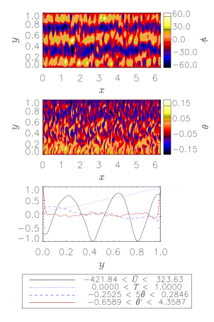
(a)  Run X: $Pr=1$, $C=0.5$, $Ra/Ra_{c}=2.75$.

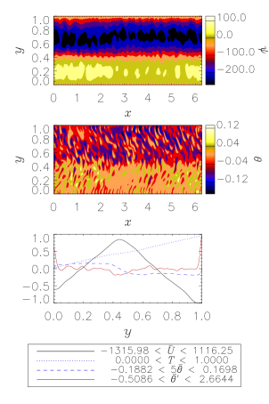
(b)  Run VII: $Pr=1$, $C=0$, $Ra/Ra_{c}=2.75$.

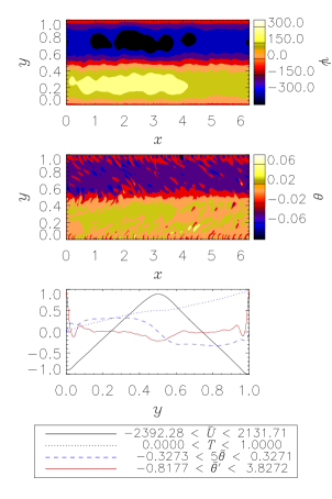
(c)  Run XV: $Pr=2$, $C=0$, $Ra/Ra_{c}=5$.

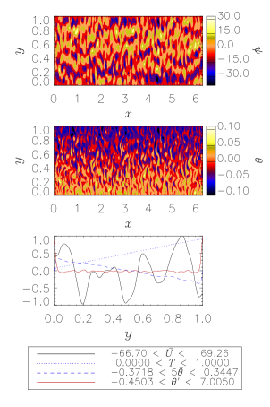
(d)  Run XVII: $Pr=2$, $C=0.5$, $Ra/Ra_{c}=2.75$.

Figure 2: Contour plots for various runs. All plots have $\beta=5\times 10^{5}$.

Many of the runs display a striking correlation of the $\theta$-contours with the slope of $\bar{U}$. The $\theta$-contours show the local slope of the flow because temperature is advected with the flow. This slope then gives the sign of the Reynolds stress, which via equation (12) determines the form of the zonal flow. Run X, displayed in figure 2(a), shows a multiple jet solution; in this case five jets are apparent located at the edges of the bands displayed in the $\psi$-plot. The $\theta$-contours show a ‘herring-bone’pattern, as the slope of the convection alternates in direction as the zonal flow alternates in sign.

The final states achieved by runs VII and XV are much the same as evidenced by the similarity of the first and third plots of figures 2(b) and 2(c). The difference in the $\theta$-plot is a result of the unsteady nature of these solutions. Both runs have settled into a bursting solution, however the snapshots of figures 2(b) and 2(c) are taken at different phases in a bursting cycle. We shall discuss this further in section III.4.

The pattern of the fields are also be affected by the Prandtl number. The convection rolls are larger at small Prandtl number and decrease in size at larger Prandtl number, which is consistent with the preferred wavenumber at onset in the limit of rapid rotation Busse and Or (1986): $k_{c}\sim(Pr/(1+Pr))^{1/3}$. It is interesting that even in this strongly nonlinear, time-dependent convection, the convection rolls follow the predicted wavenumber of linear theory. The Prandtl number still plays an important role in the pattern of convection found.

A larger Prandtl number is also beneficial to multiple jet production. Runs X, XIII and XVII each have the same (large) value of $C$ but table 2 shows that between four and seven jets are produced depending on the value of $Pr$. However, as we see from figure 2(d), the appearance of the seven jets in run XVII when $Pr=2$ is associated with a weak zonal flow. This results in the $\psi$-contours lacking a clear banded structure unlike in the equivalent case for $Pr=1$ (see figure 2(a)). Thus it seems that increasing the Prandtl number causes the system to lose its banded structure at a lower value of $C$.

The mean zonal flow is larger at small Prandtl number, and weakens at large Prandtl number. At large Prandtl number the Reynolds number of the convective flow is reduced, and this leads to a smaller zonal flow, see equation (12). The mean temperature gradients behave in the opposite manner, being weaker at low Prandtl number, because thermal diffusion is then relatively more important than advection, see equation (5). This dependence is evidenced in table 2; the most clear example is by comparing the ranges of $\bar{U}_{\text{max}}$ and $\bar{\theta}^{\prime}_{\text{max}}$ for runs VIII, XII and XV.

III.3 Rhines scaling theory

We now briefly consider the implications of the Rhines scaling theory Rhines (1975) on our results. By suggesting that the predominant balance is between the inertial and Coriolis force terms, Rhines found that the length scale of the flow should scale as $(U^{*}/\beta)^{1/2}$ for a typical flow strength of $U^{*}$, and some evidence for this scaling in the context of the convective annulus has been found Jones et al. (2003). The value for $U^{*}$ that should be used has been a topic of considerable debate due to the existence of two main typical flow strengths: the convective velocity and the zonal flow strength. Rhines originally envisaged the turbulent eddy velocity, corresponding here to the convective velocity would be used and some models of Jupiter’s jets still use this approach Schneider and Liu (2009). However an alternative view is that the zonal flow strength should be used, rather than the eddy velocity, and this has experimental Gillet et al. (2007) and numerical support Jones et al. (2003); Heimpel and Aurnou (2007).

Here we consider the applicability of the scaling theory to our results for each type of velocity separately. The convective velocity, $U_{C}$, acts in the radial direction and thus we set $U_{C}=(\max\{u_{y}\}-\min\{u_{y}\})/2$ as a measure of the convective flow strength. Similarly we set the zonal velocity, $U_{Z}$, as $U_{Z}=(\max\{\bar{U}\}-\min\{\bar{U}\})/2$. In each case the relevant quantity is also averaged over an appropriate period of time. The scaling theory stipulates that the number of jets, $M$, satisfies

$$M=c\left(\frac{\beta}{U^{*}}\right)^{1/2},$$ (16)

for some constant scaling factor, $c$. Hence for each run VII to XXV (where $\beta=5\times 10^{5}$) we are able to calculate the number of jets predicted by inserting either $U_{C}$ or $U_{Z}$ for $U^{*}$. The value of $c$ is chosen in order to best fit the actual results for the number of jets found from the numerical simulations; that is, the value of $m_{*}$.

In figure 3 we plot the number of jets predicted using the Rhines scaling theory against the actual number of jets for the two cases: $U^{*}=U_{Z}$ and $U^{*}=U_{C}$. The value of the scaling factor used is given in the caption of each plot. Exact agreement between the theory and the simulation results would result in a line of best fit with $M=m_{*}$. Figure 3(a) shows a reasonably good fit indicating that the scaling theory may well be predicting the correct length scale when the zonal velocity is used. However, it is clear from figure 3(b) that the same is not true when the convective velocity is entered as the typical flow strength. In particular, the theory is unable to predict the number of jets accurately for simulations with a large number of jets. In fact, even at low $m_{*}$ the agreement is not as consistent as figure 3(a). Consequently, we find that zonal velocities must be used in the Rhines scaling theory in order to best replicate the number of jets observed. However, due to the limited range of $\beta$ that we have tested, this conclusion really must be tested for simulations with larger rotation rates. We hope to perform this in future work.

(a)  Zonal velocity with $c=0.1345$.

(b)  Convective velocity with $c=0.1529$.

Figure 3: Plots of the true number of jets found from the simulations, $m_{*}$ against the predicted number of jets from the Rhines scaling theory, $M$, for runs VII to XXV.

When $\beta$ is held constant, equation (16) indicates that the typical flow strength must reduce in order to acquire a larger number of jets. As previously noted, multiple jets are associated with solutions that have weak zonal flow and hence the correct dependence on the flow strength is possible when $U^{*}=U_{Z}$. Conversely, the convective velocity remains at a near-constant strength regardless of the number of jets. Thus the line of best fit of figure 3(b) satisfies $M\approx$ constant and poor agreement is found between the predicted and actual number of jets.

We should note that Jones and KuzanyanJones and Kuzanyan (2009) and ChristensenChristensen (2002) found that implementing no-slip boundary conditions had the effect of removing multiple jets that were present under stress-free conditions. This is the opposite effect to that observed here, although a key difference is that their domain was spherical. Jones and KuzanyanJones and Kuzanyan (2009) and ChristensenChristensen (2002) actually found that no-slip boundary conditions reduced zonal flow to the extent that it was indistinguishable from convective velocities, so that not only were multiple jets removed but so too was any large scale zonal flow. Zonal flow production is more efficient in the annulus model compared with a spherical model. In the annulus model we have found that zonal flow is so strong with stress-free boundaries that the Rhines length fills the whole domain, precluding multiple jets. In the stress-free spherical shell models the zonal flow is relatively weaker, so according to the Rhines scaling theory Rhines (1975) the Rhines length is smaller allowing multiple jets to form. Bottom friction in the annulus model reduces the zonal flow, and hence the Rhines length, so that multiple jets can fit into the domain. No-slip boundaries in the spherical shell models weaken the zonal flow so much that it is impossible to distinguish it from the chaotic convection. It is possible that multiple jets may reappear in the no-slip spherical shell models if the Ekman number is reduced so that there is less bottom friction, but sufficiently small Ekman numbers are currently out of reach computationally. Similarly, multiple jets may appear in the stress-free annulus model at very large $\beta$ and moderate $Ra$, as the Rhines length scales as $(U/\beta)^{1/2}$. We have however been unable, so far, to reach the values of $\beta$ that may be required to observe this.

The Rhines scaling only applies when the convection is fully developed. At lower Rayleigh numbers, the bottom friction may allow multiple jets to appear because the Ekman friction term introduced when $C\neq 0$ is a scale-independent damping term. Therefore, unlike the interior viscous diffusion which dampens the small-scales more greatly than large-scale structures, the Ekman friction ‘hits’ all scales equally. This increases the likelihood of small-scale structures, such as multiple jets, appearing rather than just one large-scale equatorial jet. At Rayleigh numbers below twice critical with no bottom friction, multiple jets are damped out by the interior viscosity, even though the zonal flow is small enough that equation (16) would predict multiple jets.

III.4 The bursting phenomenon

For runs XII, VII, XV and XVII we plot, in figure 4, several more quantities as they evolve. In each figure 4(a) to 4(d) the top plot displays the various energies: the total kinetic energy, $E_{T}$, the zonal kinetic energy, $E_{Z}$, and the difference between the two, $E_{D}$ (effectively the convective energy), which were defined by equations (13 - 14). The remaining two plots contain the extremum values (that is, the maxima and minima) of the mean quantities, at each timestep. Figures 4(a) to 4(d) allow us to observe the bursting phenomenon.

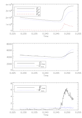
(a)  Run XII: $Pr=0.5$, $C=0$, $Ra/Ra_{c}=5$.

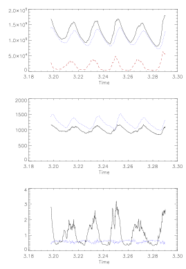
(b)  Run VII: $Pr=1$, $C=0$, $Ra/Ra_{c}=2.75$.

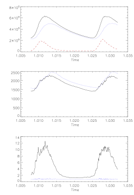
(c)  Run XV: $Pr=2$, $C=0$, $Ra/Ra_{c}=5$.

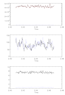
(d)  Run XVII: $Pr=2$, $C=0.5$, $Ra/Ra_{c}=2.75$.

Figure 4: Time evolution of the energy and mean quantity extrema plots for various runs. The quantities plotted are defined in panel (a).

Figure 4(b), which is for run VII, perhaps best showcases the bursts of convection, with several bursts apparent. A clear quasi-periodic phenomenon is occurring with all quantities displaying an oscillatory nature. The zonal flow is oscillating over a range of approximately 500. At times when there is a sharp increase in the energy and the extrema of $\bar{U}$, the zonal flow is driven up by the convection. However, the strong shear of the zonal flow then inhibits the convection, which depletes the source of energy for the zonal flow. Note that the maxima of the zonal energy occurs shortly after the maximum values of the extrema of $\bar{U}$. The zonal energy then decreases to a level that allows the convection to build up and a new burst can occur.

The physical mechanism by which the zonal flow actually suppresses the convection has not been much discussed. We have performed a linear stability analysis for the annulus model with a linear flow pattern imposed in the basic state in a similar manor to that of Teed et al.Teed et al. (2010). We find that the critical Rayleigh number always increases with increasing flow strength confirming that zonal flow inhibits convection. We also find that the critical wavenumber is substantially reduced, so longer waves are preferred. The temperature perturbation of short wavelength cells is disrupted by the shear. In mathematical terms, the large zonal flow means that the temperature perturbation $\theta$ in equation (5) must be small for the term $\bar{U}\partial\theta/\partial x$ to balance the advection down the mean temperature gradient $-\partial\psi/\partial x$ and the temperature diffusion $\nabla^{2}\theta$, but small temperature perturbations require very large $Ra$ to provide sufficient buoyancy. In practice, the system responds by choosing a longer wavelength parallel to the zonal flow (small $k$) to reduce the effect of the $\bar{U}\partial\theta/\partial x$ term, but this is not optimal for rapidly rotating convection which prefers large $k$. So the critical Rayleigh number is increased in the presence of shear. Note that this argument only applies to modes which are buoyancy driven, as modes which are driven by the shear itself do not rely on the temperature perturbation. However, modes driven by shear flow instability do not seem to play a big role in our simulations. Note also that it is shear which disrupts the temperature perturbation. If there is a large constant zonal flow $\bar{U}$, then waves with phase velocity $\approx\bar{U}$ can happily grow, but if the large velocity $\bar{U}$ varies with position, it is not possible for a single phase speed $c$ to cancel out $\bar{U}$ everywhere in equation (5).

Table 2 indicates the runs for which bursting was observed with the range of the zonal flow also displayed. We find that as $C$ is increased from zero, in runs IX and X, bursting ceases and the range of the oscillations of the zonal flow is smaller (compare with run VII). Therefore, we can conclude that the bottom friction hinders the bursting phenomenon, which is in agreement with the previous work (Jones et al., 2003; Rotvig and Jones, 2006). For the runs where bursting occurs for $Pr=1$ (that is, runs VII, VIII and XXIV) the period of the bursting is found to be $\approx 0.02$ of a diffusion time. This can be observed from figure 4(b).

When $Pr=0.5$ we see, from table 2 that the strength and range of the zonal flow is small for run XI where $Ra=2.75Ra_{c}$. However, when the Rayleigh number is increased to five times critical in figure 4(a), for run XII, the zonal energy forms the majority of the kinetic energy in the system. There is also evidence of the bursting phenomenon with a gradual decline in all of the quantities in the three plots before a sharp increase at $t\approx 2.48$. Bursting also continues to be found in run XXV where $Ra/Ra_{c}=10$. Therefore the possibility of convective bursts exists at $Pr=0.5$ so long as the driving is large enough.

In figures 4(c) and 4(d) we plot the energy and mean quantity extrema plots for runs XV and XVII where $Pr=2$. Figure 4(c) once again shows clear evidence of bursting, this time at five times critical, with significant fluctuations in both mean quantities. The maximum values of $E_{T}$ and $\bar{\theta}^{\prime}_{\textrm{max}}$ occur shortly before the peaks in $\bar{U}_{\textrm{max}}$ and $-\bar{U}_{\textrm{min}}$. The period of time between bursts has also remained constant at $\approx 0.02$ despite the increase in the Prandtl and Rayleigh numbers compared with run VII. This suggests that the period of the bursts may not be strongly dependent on either $Pr$ or $Ra$. From figure 4(c) it is clear that the snapshot for this run (see figure 2(c)) is taken during a time of strong zonal flow; that is a post-convective burst. The convection in figure 2(c) is also localized due to the strong zonal flow. This is in contrast to figure 2(b) which is taken during a burst. This shows that during a bursting cycle there are both periods where convection occurs everywhere and where convection is localized. This is a common attribute of all bursting runs. Also of note is that the range of the fluctuation in the maximum value of the mean temperature gradient is larger than in the cases of lower Prandtl number (compare with figure 4(a)). Figure 4(d), for run XVII where $C=0.5$, again shows that increasing the bottom friction causes the bursting to halt, as well as reducing the magnitude of the zonal flow itself.

At $Pr=5$ we find that, despite the zonal energy forming the majority of the kinetic energy, the bursting ceases. The extremely small range of the zonal flow for run XVIII in table 2 indicates that the values of these quantities are nearly constant over a long period of time. The same situation was found for run XIX, which has a larger Rayleigh number so bursting does not occur even for values of $Ra$ that are several times critical. No bursting was observed for runs with $Ra/Ra_{c}=2.75$ and $Pr=0.2$. With the non-zero values of $C$ used in runs XXI and XXII, the zonal flow is weak, so bursting would not be expected. In run XX, $C=0$ and the zonal flow is quite strong, but no bursting was found. However, increasing the Rayleigh number to five times critical in run XXIII, produces bursting although the oscillations are significantly weaker than those found for equivalent parameters in the $Pr=0.5$ case. This suggests that the onset of bursting is delayed as the Prandtl number is decreased.

In the annulus problem, bursting can be thought of as temporal intermittency, but in other geometries spatial intermittency can also occur. Spatial intermittency is sometimes referred to as ‘nests of convection’ Brown et al. (2008). Spatial intermittency can occur in two different ways. It can occur with temporal intermittency, that is when the burst occurs it onsets preferentially in the neighborhood of a particular longitude. We see this happening in the annulus model, but typically the burst soon spreads out throughout the whole domain. More localized bursts have been seen in spherical shell geometry Heimpel and Aurnou (2012); Ballot et al. (2007). However, in spherical shell geometry persistent nests of convection can occur, both in Boussinesq Grote and Busse (2001) and in anelastic convection Brown et al. (2008). In this configuration, convection only occurs in patches which drift azimuthally in longitude, while individual convection columns drift through the patch, growing as they enter the patch and decaying as they leave it. We have not seen this phenomenon in the annulus model. In spherical geometry, the Rossby waves propagate faster in the outer parts of the shell, where the boundary slope is steeper, and more slowly in the deep interior where the slope is shallower. In the annulus model the boundary slope is constant, so this differential propagation speed with radius does not occur, which maybe why we did not find persistent nests of convection in the annulus.

IV Mean field stability theory

In the previous section, we saw how large zonal flows and mean temperature gradients readily appeared under many parameter regimes. It is desirable to explore the disruptive effects that these mean quantities have on the convection in order to better explain how the bursts occur. Perhaps the most informative method is to consider a linear theory with the mean quantities derived from the nonlinear code used to define a basic state from which the growth rates of convection can be observed. This is what we analyze in this section.

We consider a zonal flow, $\mathbf{u_{0}}=U_{0}(y)\mathbf{\hat{x}}$ and a mean temperature profile, $T_{0}+G_{0}(y)$, to be included in the basic state. $G_{0}(y)$ measures the departure of the mean temperature from the conduction state. Perturbations $\tilde{\psi}$ and $\tilde{\theta}$ around this basic state satisfy

$$\frac{\partial\nabla^{2}{\tilde{\psi}}}{\partial t}+ReU_{0}\frac{\partial\nabla^{2}{\tilde{\psi}}}{\partial x}-(\beta+ReU_{0}^{\prime\prime})\frac{\partial{\tilde{\psi}}}{\partial x}=-Ra\frac{\partial{\tilde{\theta}}}{\partial x}-C|\beta|^{1/2}\nabla^{2}{\tilde{\psi}}+\nabla^{4}{\tilde{\psi}},$$ (17)

$$Pr\left(\frac{\partial{\tilde{\theta}}}{\partial t}+ReU_{0}\frac{\partial{\tilde{\theta}}}{\partial x}+\frac{\partial{\tilde{\psi}}}{\partial x}\frac{\mathrm{d}G_{0}}{\mathrm{d}y}\right)=-\frac{\partial{\tilde{\psi}}}{\partial x}+\nabla^{2}{\tilde{\theta}},$$ (18)

with the introduction of terms involving $U_{0}$ and $G_{0}$. Disturbances have $\exp(ikx)$ dependence, $k$ being the wavenumber in the $x$-direction. We have non-dimensionalized the zonal flow by assuming that it has a typical velocity, $U^{*}$, to give a Reynolds number

$$Re=\frac{DU^{*}}{\nu}.$$ (19)

This linear problem is solved using the same method as in Teed et al.Teed et al. (2010). No assumption has yet been made regarding the form of $U_{0}$ or $G_{0}$. However, now we use the runs discussed in section III to provide the mean quantities to be entered into the linear theory. Of course, as the system is evolved during these runs the zonal flow and mean temperature change at each timestep. In order to fully analyze the effects of the mean quantities on the linear theory we perform the linear stability analysis at each timestep, which allows us to see how the growth rates of the linear system vary as the dynamics of the nonlinear system evolve. Therefore we add a subroutine to the nonlinear code, which solves the linear stability problem at each timestep. With the same parameter set as that being used in the nonlinear run and with $U_{0}(y)$ and $G_{0}(y)$ set equal to $\bar{U}$ and $\bar{\theta}$ respectively, the subroutine outputs the largest growth rate, as well as the corresponding frequency, $\omega$, and wavenumber, $k$. We set $Re=1$ so that the magnitude of the zonal flow comes solely from the nonlinear simulations. We expect that the growth rate will be large when a burst arises. Conversely, when the zonal flow is strong the expectation is that the growth rate will attain a minimum due to the disruption of convection by zonal flow as we discussed in section III.4. In order for convection to cease we expect to find marginal growth rates at times of large $\bar{U}$. The idea we explore is that it is the small scale convection which drives the zonal flow and the mean temperature gradient, but for much of the time these mean quantities are such that convective instability is suppressed. When these mean quantities have weakened through diffusive effects, we expect to see positive growth rates for convective instability, and the onset of a burst of convection.

In the plots that we shall discuss, the growth rate, wavenumber and frequency will be functions of time. We are primarily interested in the growth rate of the fastest growing mode and how it varies as the nonlinear system is evolved. This is because we wish to ascertain if the magnitude of growth is at all correlated with the mean quantities. Consequently, we primarily look at the linear outputs for runs of section III where the bursting phenomenon was witnessed. In particular, we discuss results from the linear theory for the same time intervals and runs as those taken for the plots in figure 4, in order to ease comparison.

IV.1 Linear results with nonlinear zonal flow

We begin with the case where only the zonal flow, $\bar{U}$, is included in the linear theory. Hence in this subsection we set $U_{0}(y)=\bar{U}(y)$ and $G_{0}(y)=0$ in the linear equations (17-18). Figure 5 shows how the growth rate, $\sigma$, frequency, $\omega$, and wavenumber, $k$, vary as the nonlinear system is evolved, for the runs for which plots were produced in figure 4.

Figure 5(a), for run XII, can be compared with the plots of figure 4(a). The zonal energy of figure 4(a) is shown as a dotted line to aid comparison. As the zonal flow strength gradually decreases the quantities plotted in figure 5(a) remain fairly constant. However, there is a sudden increase in $\sigma$ and $k$ at $t\approx 0.247$, which is where $E_{Z}$ attains its minimum. This is expected as the growth of convection should occur when the zonal flow is weakest. Although the range of the growth rate is quite large, we notice that $\sigma$ is never less than $\approx 1500$. Therefore the zonal flow reduces the growth of the convection but does not completely cause it to cease. The zonal flow $E_{Z}$ increases strongly following the burst of convection after $t\approx 0.247$, and the growth rate begins to decrease again due to the disruption of the convection by the additional strength of the zonal flow.

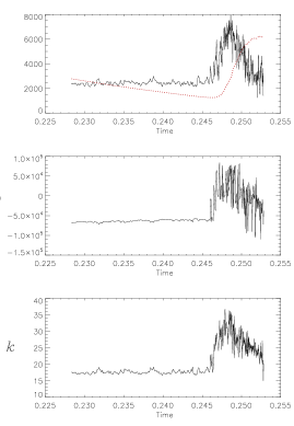
(a)  Run XII.

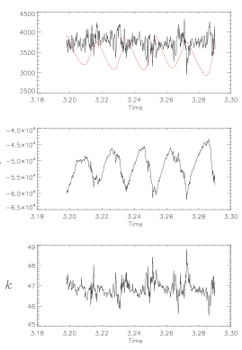
(b)  Run VII.

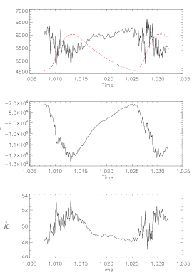
(c)  Run XV.

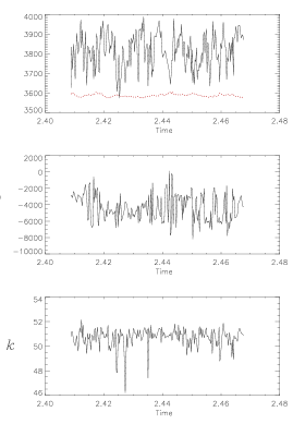
(d)  Run XVII.

Figure 5: Time evolution of the growth rate, frequency and wavenumber plots for runs with only nonlinear zonal flow. The dotted line is the energy of the zonal flow.

Unlike in the case for run XII, the growth rate in figure 5(b) remains relatively constant. The correlation with $E_{Z}$ in figure 4(b) is also far less obvious, so it seems again that the zonal flow is not sufficiently affecting the growth of convection. There is excellent correlation however between the frequency, $\omega$, and the zonal flow strength. The frequency is smallest in magnitude when the zonal flow is weakest. Peaks in $k$ also coincide with locations of strong zonal flow although the range of the wavenumber is small. Run XV also displays bursting and again there is correlation between the quantities of figures 5(c) and 4(c). Once again the minimum growth rate is attained when the zonal energy is largest but the zonal flow is unable to reduce the growth rate to marginal or decaying modes. When comparing figures 5(d) and 4(d) we immediately notice the lack of correlation between quantities that was present for the previous runs discussed and thus the departure from the $U_{0}=0$ case is minimal. This is to be expected since run XVII is not a bursting solution and is included here simply as an example of a non-bursting run.

We can conclude from this subsection that the zonal flows of the nonlinear theory certainly have a profound effect on the linear growth rates of convection. However, the zonal flow is unable to halt the growth of convection altogether as evidenced by the lack of negative growth rates in figure 5. Therefore another process, at least in part, must be responsible for the sufficient reduction in convective growth.

IV.2 Linear results with nonlinear mean temperature gradient

We now consider the linear stability results in the absence of any zonal flow but with the mean temperature profile, $\bar{\theta}$, included. Thus, in this subsection we set $U_{0}=0$ and $G_{0}=\bar{\theta}$ in the linear equations (17-18). Figure 6 contains plots displaying how $\sigma$, $\omega$ and $k$ vary as the nonlinear system is evolved when only the mean temperature gradient is included in the linear system. We show also the zonal flow energy, which varies smoothly and is well-correlated with the mean temperature gradient.

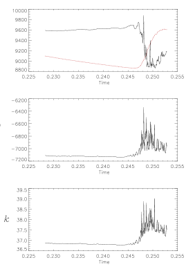
(a)  Run XII.

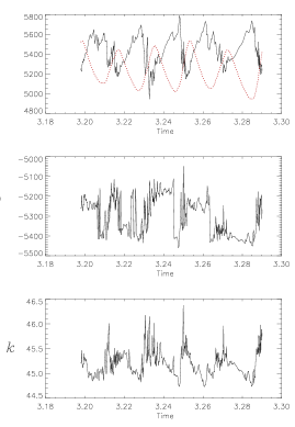
(b)  Run VII.

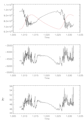
(c)  Run XV.

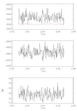
(d)  Run XVII.

Figure 6: Time evolution of the growth rate, frequency and wavenumber plots for runs with only nonlinear mean temperature gradient. The dotted line is the energy of the zonal flow, included since the mean temperature gradient is well correlated with the zonal flow.

All three of the quantities in figure 6(a) remain near-constant to begin with since the extrema of the mean temperature gradient are also approximately constant for $t<0.247$ (compare with figure 4(a)). The sudden increase in $\bar{\theta}^{\prime}_{\textrm{max}}$ at $t\approx 0.247$ is accompanied by an abrupt reduction in the growth rate. This is to be expected since if the mean temperature gradient is able to partially (or indeed, fully) cancel out the static temperature gradient, the overall gradient will be less adverse. Thus the system will be less eager to convect, resulting in a lowering of the growth rate. However, even when the mean temperature gradient is strong the growth rate is only reduced by approximately $10\%$. In fact, this is a smaller reduction of the growth rate than was present in the previous subsection. Associated with the region of strong mean temperature gradient, there is a reduction in $|\omega|$ and the wavelengths of the modes.

The plots in figure 6(b), for run VII, show clear correlation with 4(b). The growth rate oscillates, though again does not reduce significantly. The correlation of the frequency and wavenumber is also clear with the same dependence as seen before. In figure 6(c), for run XV, we again see the same pattern of correlation by comparing with figure 4(c). Peaks of $\bar{\theta}^{\prime}_{\textrm{max}}$ at $t\approx 1.012$ and $t\approx 1.029$ are associated with weak growth and short wavelengths whilst the intermediate period has increasing growth. The plots for run XVII, displayed in figure 6(d), display only small fluctuations in $\sigma$, $\omega$ and $k$. This is to be expected since the values of the extrema of the mean temperature gradient are near-constant in this non-bursting solution (see figure 4(d)).

We have found that a strong mean temperature gradient can indeed reduce the growth rate of convection due to a reduction in the overall adverse temperature gradient present. However, the growth rate does not become marginal or negative even during times of strong mean temperature gradient.

IV.3 Linear results with both nonlinear mean quantities

We now finally consider the linear stability results with both mean quantities, $\bar{U}$ and $\bar{\theta}$, included in the basic state since we expect that both a zonal flow and a mean temperature gradient are necessary to produce the bursting phenomenon. Therefore in this subsection we set $U_{0}=\bar{U}$ and $G_{0}=\bar{\theta}$ in the linear equations (17-18).

The comparison of figure 7(a), for run XII, with figure 4(a) shows that there is again correlation between the linear quantities and the nonlinear energies. In fact, the plots of figure 7(a) are extremely similar to those of figure 5(a) where only a basic state zonal flow was included. Strong growth of the same order of magnitude remains possible at times when the zonal flow and mean temperature gradient are weak. However, the key difference between these sets of plots is that, for the case where both mean quantities are included, the growth rate is approximately zero when the mean quantities are large. This was not the case previously and therefore including both mean quantities has given the desired result which is the ceasing of the convection.

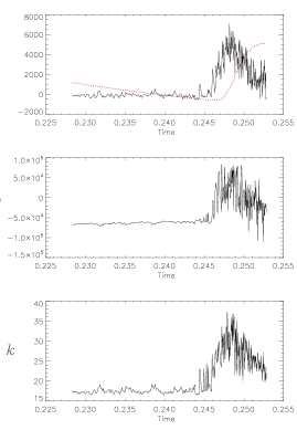
(a)  Run XII.

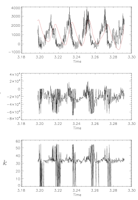
(b)  Run VII.

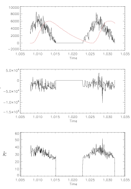
(c)  Run XV.

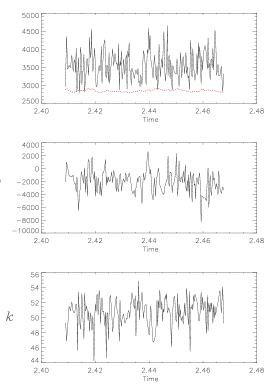
(d)  Run XVII.

Figure 7: Growth rate, frequency and wavenumber plots for runs with zonal flow and nonlinear mean temperature gradient.

The correlation of $\sigma$ in figure 7(b), for run VII, with the quantities plotted in figure 4(b) is striking. As with figure 6(b) there is strong growth located where the zonal flow and mean temperature gradient are weak. However, unlike figures 5(b) and 6(b), the growth rate becomes negative when it attains its minimum values. Hence when the mean quantities are large the convective modes of the linear theory decay. Figure 7(c), for run XV, also appears to show that both mean quantities are necessary for bursting. There is an initial period of strong growth at $t\approx 1.010$ where we see from figure 4(c) that the mean quantities are weak. Followed by the strong growth there is a period where $\sigma\approx 0$ coinciding with the time between which $E_{Z}$ reduces from its maxima to its minima. After the zonal energy attains its minimum value, the zonal flow is weak enough to allow a second period of strong growth located at $t\approx 1.026$. Also of interest in both figures 7(b) and 7(c) is that $k$ and $\omega$ tend to zero during periods of weak growth. The marginal modes, found when the mean quantities are strong, are therefore steady in these cases. The plots displayed in figure 7(d) are similar to those found for the non-bursting run XVII in the previous subsections. Once again all three quantities take (non-zero) near-constant values as expected, due to the weak mean quantities for run XVII.

We can conclude from this subsection that it appears that the necessary condition for bursts of convection is the existence of both a zonal flow and a mean temperature gradient. We have observed marginal growth rates in all three runs that admit bursting. The Rayleigh number in all runs is several times critical. Thus, when the mean quantities are strong and of the correct form, they are able to reduce the system to near-onset behavior.

V Conclusions

The results of our nonlinear annulus model produced good agreement with previous simulations Jones et al. (2003) and zonal flows were found to readily occur. Multiple jets and a periodic nature of convection appearing in bursts can be found under certain parameter regimes. However, bursting multiple jet solutions were not observed at any Prandtl number, extending the idea that multiple jets and bursts are likely to be mutually exclusive phenomena Rotvig and Jones (2006) to cases with $Pr\neq 1$. Rigid top and bottom boundaries are preferable for multiple jets whereas bursts of convection certainly prefer stress-free boundaries. Zonal flows are also found to be weaker with rigid boundaries implemented. We also found fluctuations in the mean temperature gradient on a similar timescale to the bursts of convection which have not been addressed in the previous literature. We found reasonable agreement with the Rhines scaling theory Rhines (1975) only when the zonal velocity was using in the scaling. It seems that the convective velocity is unable to predict the correct number of jets although further parameter regimes, including with larger values of $\beta$, should be tested confirm this result.

As an extension to the previous work, we performed runs with $Pr\neq 1$. In general, increasing the Prandtl number depletes the strength of the zonal flow. The bursts of convection appear to be a phenomenon most frequently observed at $Pr=1$ agreeing with previous work Christensen (2002). Although we found that bursts were possible at a range of Prandtl numbers, the onset of bursting appears to be delayed to larger Rayleigh numbers if the Prandtl number is not unity. This was most notably confirmed at $Pr=0.2$ by the lack of bursts at $Ra/Ra_{c}=2.75$ and the appearance of only very weak bursting at $Ra/Ra_{c}=5$. At even larger Rayleigh numbers the convection becomes highly chaotic. Therefore it appears that the bursting phenomenon may be restricted to an ever shrinking window of parameter space as the Prandtl number is reduced. At low enough Prandtl number the bursting regime may be omitted altogether restricting the phenomenon to a finite range of $Pr$. This will have to be tested in future work.

Physically, the zonal flow certainly disrupts the convection as expected and as observed in section IV.1. Similarly, the introduction of a strong mean temperature gradient can result in the reduction of the overall temperature gradient, $T^{\prime}=\Delta T/D+\bar{\theta}^{\prime}$. The adverse temperature gradient must exceed some value in order for convection to be beneficial. Also, the steeper the adverse temperature gradient the stronger the resulting convection will be. Hence a partial cancellation of the static temperature gradient, $\Delta T/D$, will also weaken the convection. We believe that the shearing of the zonal flow, coupled with the partial balancing of the adverse temperature gradient, is the requirement to halt convection. This is in contrast to previous work on the subject where it was believed that the zonal flow could sufficiently disrupt the convection to cause bursts. Both the zonal flow strength and the mean temperature gradient must also exceed some critical value in order for the convection to cease. In the case of the zonal flow the shearing must be great enough and in the case of the mean temperature gradient the static temperature gradient must be sufficiently balanced. When this occurs, the driving force of both of the mean quantities is removed. Consequently, there is a depletion in the strength of the zonal flow and the temperature gradient reverts to approximately that of the static case so that convection is once again beneficial and a burst occurs. This argument also offers an explanation as to why bursting is preferentially observed at Prandtl number of order unity. At high Prandtl number, the zonal flow is too weak for bursting, and at low Prandtl number, although the zonal flow is strong, the mean temperature is too close to its conduction state value.

It is not currently known if the jets of the gas giants possess a periodic nature. The parameter regimes we have tested suggest it may be unlikely that the multiple jet structure of the Jovian atmosphere can coexist with bursts of convection. However, if the high latitude jets are driven by a different process to that of the strong equatorial jets Heimpel et al. (2005); Heimpel and Aurnou (2007), it may be that some but not all jets display an oscillation in the zonal flow strength. Further observations of the wind speeds of the jets of the gas giants over time is required. The Juno mission which launched in August 2011 will be placed in a polar orbit of Jupiter in order make further observations of the planet including their jet speeds Matousek (2007).