Metric deformation and boundary value problems in 3D

Abstract

A novel perturbative method, proposed by Panda et al. [1] to solve the Helmholtz equation in two dimensions, is extended to three dimensions for general boundary surfaces. Although a few numerical works are available in the literature for specific domains in three dimensions such a general analytical prescription is presented for the first time. An appropriate transformation is used to get rid of the asymmetries in the domain boundary by mapping the boundary into an equivalent sphere with a deformed interior metric. The deformed metric produces new source terms in the original homogeneous equation. A deformation parameter measuring the deviation of the boundary from a spherical one is introduced as a perturbative parameter. With the help of standard Rayleigh-Schrödinger perturbative technique the transformed equation is solved and the general solution is written down in a closed form at each order of perturbation. The solutions are boundary condition free and which make them widely applicable for various situations. Once the boundary conditions are applied to these general solutions the eigenvalues and the wavefunctions are obtained order by order. The efficacy of the method has been tested by comparing the analytic values against the numerical ones for three dimensional enclosures of various shapes. The method seems to work quite well for these shapes for both, Dirichlet as well as Neumann boundary conditions. The usage of spherical harmonics to express the asymmetries in the boundary surfaces helps us to consider a wide class of domains in three dimensions and also their fast convergence guarantees the convergence of the perturbative series for the energy. Direct applications of this method can be found in the field of quantum dots, nuclear physics, acoustical and electromagnetic cavities.

I Introduction

The three dimensional Helmholtz equation is encountered frequently by physicist and engineers in different areas $-$ like the eigenanalysis in acoustic and electromagnetic cavities, transmission of acoustic waves through ducts and in quantum mechanics. The main concern to pursue these problems is to calculate the eigenspectrum of the linear homogeneous Helmholtz equation for different boundary conditions and geometries. In the acoustic wave motion, for the sinusoidal variation of the sound pressure with time, wave equation transforms to the standard Helmholtz equation. Also in the quantum scenario, for stationary problems the unitary evolution of the wavefunction reduces the Schrödinger equation into the Helmholtz equation. Notable example of the Dirichlet boundary condition (DBC) is the confinement of a quantum particle in an infinite potential well where the eigenfunction vanishes on the boundary. A nucleon in the nucleus can be treated as this in the first approximation neglecting its interaction with the other nucleons. Canonical example of Neumann boundary condition (NBC) is the acoustic cavity where the sound velocity (which is proportional to the gradient of the sound pressure) is set to zero on the boundary. In order to find a solution of the particular partial differential equation (PDE) we have to select, from all the possible solutions of the aforesaid equation, the specific combination which will respect the boundary condition. Now these particular problems become different in the nature of the boundary conditions imposed; either the geometry of the boundary varies or the specific behaviour of the eigenfunction at the boundary is different. So to categorise the solution of a particular PDE, say the Helmholtz equation for our case, depending on the shapes of the boundary surface and also according to the nature of the boundary condition is an intricate task. For a restricted class of domains with simple geometries in three dimensions, viz. rectangular, spherical and cylindrical, analytic closed form solutions are available [2, 3]. Constructing on the boundary a co-ordinate system suitable to it often helps in finding the solution. For the Helmholtz equation in three dimensions, there are $11$ such `special' co-ordinate systems [4]. However, even in these sacred classes, the multi-parameter dependence of the solution makes them difficult to use. So, for a general domain, finding solutions to the Helmholtz equation becomes a formidable job. However, many physical problems demand us to solve the equation for an arbitrary domain which is significantly deviated from the above mentioned idealised scenario. In particular, the geometry of the nanoscale second-phase particles are described analytically as superellipsoids [5] and experimentally verified from just one micrograph [6]. To explore the shapes of these particles more accurately, we need a good estimation of the eigenspectra of these geometries which urge us to solve the Helmholtz equation for these arbitrary boundaries. Recently in the field of medical science for automatic prostate segmentation using deformable superellipses have been efficiently applied [7]. The analytic approach towards this problem came recently by Panda and Hazra [8] where they have generalised Rayleigh's theorem in three dimensions and used the standard time independent perturbation method of quantum mechanics to calculate the eigenfunction and eigenvalue corrections in closed forms up to the second order of perturbation for general shapes in three dimension in terms of the spherical harmonics expansion coefficients. Most of the earlier attempts made towards this problem were via numerical means in the area of chaos for general three dimensional billiards [9, 10, 11, 12, 13, 14] and also in some recent experiments to study the wave chaos in microwave [15] and resonant optical cavities [16]. Among the numerical schemes, the finite difference method (FDM), the finite element method (FEM) [17] and the boundary element method (BEM) [18] are popular ones but they consume huge amount of time to generate the mesh for a complicated geometry. Recently as alternatives to the above, some meshless methods have been developed, like the boundary collocation method [19], the radial basis function [20], the method of particular solutions [21] and the method of fundamental solutions [22]. These methods also have the drawback of getting spurious eigensolutions.

In this paper, we have prescribed an alternative method to solve the boundary value problem for the Helmholtz equation for a general simply connected convex domain in three dimensions. This analytic formulation is an extension of our earlier work for two dimensions [1] where a suitable diffeomorphism in terms of a Fourier series was chosen to map the general problem into an equivalent one where the boundary was circular but the equation gets complicated due to the deformation of the metric in the interior and was solved by perturbation technique of quantum mechanics. In this method, an arbitrary domain in three dimensions is mapped to a regular closed region (in which the Helmholtz equation is exactly solvable) by a suitable co-ordinate transformation resulting the deformation of the interior metric. As a result, the homogeneous Helmholtz equation gets modified and can be written as the original one with additional source terms present on the right hand side of it. These extra terms can now be treated as a perturbation to the original equation and is solved using the standard perturbation technique. The corrections to the eigenfunction are obtained in closed form at each order of perturbation irrespective of the boundary conditions. The eigenvalue correction at each order is calculated by applying the proper boundary conditions on the respective eigenfunction corrections. To be able to express the eigenfunction corrections independent of the boundary conditions is a unique advantage of this method over the existing ones. Also, in this method the boundary conditions maintain a simple form at each order of perturbation and is easy to apply on some regular closed surface. In this analysis, we have used spherical harmonics to represent the asymmetries of the boundary from its equivalent sphere which allows us to implement the method for a large variety of geometries in three dimensions. To test the efficacy of the perturbative method we have tabulated the analytical values with the corresponding numerical ones for spheroids, supereggs, stadium of revolution, rounded cylinder and pear shaped enclosures. The method seems to work extremely well for these cases for both Dirichlet and Neumann conditions. It has a potential of applicability for various general shapes in three dimensions, where the deviations are large from a spherical shape.
The paper is organised as follows : the section II describes the general formalism in the abstract sense. In section III, we have applied the method to various enclosures. The last section IV is reserved for results, conclusions and comments.

II Formulation

The homogeneous Helmholtz equation reads,

$$\left(g_{ij}\nabla^{i}\nabla^{j}+k^{2}\right)\psi\equiv\left(\triangle+{\cal E}\right)\psi=0,$$ (1)

where $g_{ij}$ is the background metric component on three dimensional space ($\cal V$) and $\nabla$ represents a covariant derivative. $\triangle$ is the Laplacian operator in three dimensions. Our interest lies in finding the eigenspectrum and the solutions in the interior of a closed simply connected convex region satisfying either the Dirichlet boundary condition (DBC), $\psi=0$, or the Neumann boundary condition (NBC), $\frac{\partial\psi}{\partial n}=0$, on the boundary $\partial\cal V$, where $\frac{\partial\psi}{\partial n}$ is the derivative along the outward normal direction to $\partial\cal V$. Depending on the boundary condition the parameter $k^{2}$ can be matched to a physical quantity (for the DBC it is proportional to the energy of a quantum particle confined within $\partial\cal V$, where as for the NBC it will determine the square of the resonating frequencies for acoustical cavities).

For convenience, we choose to work in spherical polar coordinate system ($R,\Theta,\Phi$). Now, We consider a general arbitrary surface of the form $R=R(\Theta,\Phi)$. The periodicity condition implies that $R(\Theta,\Phi+2\pi)=R(\Theta,\Phi)$. We assume that any general shape (which is not very elongated in one direction) can be expressed as a deformation around an effective spherical boundary. We choose spherical boundary because the Helmholtz equation in 3D is exactly solvable for this boundary (the analysis in principle can work for perturbation around any simple surface for which the Helmholtz equation is exactly solvable). We make a coordinate transformation from the old one $(R,\Theta,\Phi)$ to a new one $(r,\theta,\phi)$ of the form

$$R=r\leavevmode\nobreak\ (1+\epsilon f(\theta,\phi))$$ (2a)

$$\Theta=\theta$$ (2b)

$$\Phi=\phi$$ (2c)

where $\epsilon$ is a deformation parameter. Now, for an intelligent choice of the well behaved function $f(\theta,\phi)$, our arbitrary surface will be transformed into a sphere of average radius,

$$R_{0}=\frac{1}{4\pi}\int\limits_{0}^{\pi}\int\limits_{0}^{2\pi}R(\theta,\phi)\sin\theta\text{d}\theta\text{d}\phi,$$ (3)

in the $(r,\theta,\phi)$ system. As a result of the deformation, there will be changes in the underlying metric component $g_{ij}(R,\Theta,\Phi)$. Henceforth, we use the notation

$$f^{(i,j)} \equiv\frac{\partial^{i+j}f}{\partial\theta^{i}\partial\phi^{j}}.$$

The dependence on the arguments $(\theta,\phi)$ is not shown explicitly for brevity. The flat background metric in the old coordinate system ($R,\Theta,\Phi$) is given by $g={\rm diag}\,(1,R^{2},R^{2}\sin^{2}\Theta)$. Under the coordinate transformations (2) it takes the form

$$\tilde{g}=\left(\begin{array}[]{lcc}(1+\epsilon f)^{2}&r\epsilon(1+\epsilon f)f^{(1,0)}&r\epsilon(1+\epsilon f)f^{(0,1)}\\ r\epsilon(1+\epsilon f)f^{(1,0)}&r^{2}\left[(1+\epsilon f)^{2}+\epsilon^{2}f^{{(1,0)}^{2}}\right]&r^{2}\epsilon^{2}f^{(0,1)}f^{(1,0)}\\ r\epsilon(1+\epsilon f)f^{(0,1)}&r^{2}\epsilon^{2}f^{(0,1)}f^{(1,0)}&r^{2}\left[(1+\epsilon f)^{2}\sin^{2}\theta+\epsilon^{2}f^{{(0,1)}^{2}}\right]\end{array}\right).$$

The non-vanishing components of connection $\Gamma$ for the flat background metric ($g$) given by,

$$\begin{array}[]{lll}\Gamma^{R}_{\phantom{r}\Theta\Theta}=-R,&\Gamma^{\Theta}_{\phantom{r}R\Theta}=\frac{1}{R},&\Gamma^{\Phi}_{\phantom{r}R\Phi}=\frac{1}{R},\\ \Gamma^{R}_{\phantom{r}\Phi\Phi}=-R\sin^{2}\Theta,&\Gamma^{\Theta}_{\phantom{r}\Phi\Phi}=-\cos\Theta\sin\Theta,&\Gamma^{\Phi}_{\phantom{r}\Theta\Phi}=\cot\Theta,\end{array}$$

modify to

$$\Gamma^{r}_{\phantom{r}\theta\theta}=\leavevmode\nobreak\ -r\left[1-\frac{\epsilon f^{(2,0)}}{(1+\epsilon f)}+\frac{2\epsilon^{2}f^{{(1,0)}^{2}}}{(1+\epsilon f)^{2}}\right],\leavevmode\nobreak\ \Gamma^{r}_{\phantom{r}\theta\phi}=\leavevmode\nobreak\ \epsilon r\left[\frac{\left(f^{(1,1)}-f^{(0,1)}\cot\theta\right)}{(1+\epsilon f)}-\frac{2\epsilon f^{(1,0)}f^{(0,1)}}{(1+\epsilon f)^{2}}\right],$$

$$\Gamma^{r}_{\phantom{r}\phi\phi}=\leavevmode\nobreak\ -r\left[\sin^{2}\theta-\frac{\epsilon\left(f^{(0,2)}+\cos\theta\sin\theta f^{(1,0)}\right)}{(1+\epsilon f)}+\frac{2\epsilon^{2}f^{{(0,1)}^{2}}}{(1+\epsilon f)^{2}}\right],\leavevmode\nobreak\ \Gamma^{\theta}_{\phantom{r}r\theta}=\frac{1}{r},\leavevmode\nobreak\ \Gamma^{\theta}_{\phantom{r}\theta\theta}=\frac{2\epsilon f^{(1,0)}}{1+\epsilon f}$$

$$\Gamma^{\theta}_{\phantom{r}\theta\phi}=\frac{\epsilon f^{(0,1)}}{1+\epsilon f},\leavevmode\nobreak\ \Gamma^{\theta}_{\phantom{r}\phi\phi}=-\cos\theta\sin\theta,\leavevmode\nobreak\ \Gamma^{\phi}_{\phantom{r}r\phi}=\frac{1}{r},\leavevmode\nobreak\ \Gamma^{\phi}_{\phantom{r}\theta\phi}=\cot\theta+\frac{\epsilon f^{(1,0)}}{1+\epsilon f},\leavevmode\nobreak\ \Gamma^{\phi}_{\phantom{r}\phi\phi}=\frac{2\epsilon f^{(0,1)}}{1+\epsilon f}.$$

As a result of the coordinate transformation (2) no spurious curvature is induced in the manifold (i.e. Riemann tensor, $R^{i}_{{\phantom{i}}jkl}=0\leavevmode\nobreak\ \leavevmode\nobreak\ \forall\leavevmode\nobreak\ i,j,k,l$). Under the map $(R,\Theta,\Phi)\rightarrow(r,\theta,\phi)$, Eq. (1) takes the following form

$$\frac{1}{r^{2}(1+\epsilon f)^{4}}\left[\cot\theta(1+\epsilon f)^{2}\psi^{(0,1,0)}+r\left\{2(1+\epsilon f)^{2}-\epsilon(1+\epsilon f)\left(\frac{f^{(0,2)}}{\sin^{2}\theta}+\cot\theta f^{(1,0)}+f^{(2,0)}\right)\right.\right.$$

$$\left.\left.+2\epsilon^{2}\left(\frac{f^{{(0,1)}^{2}}}{\sin^{2}\theta}+f^{{(1,0)}^{2}}\right)\right\}\psi^{(1,0,0)}+r^{2}\left\{(1+\epsilon f)^{2}+\epsilon^{2}\left(\frac{f^{{(0,1)}^{2}}}{\sin^{2}\theta}+f^{{(1,0)}^{2}}\right)\right\}\psi^{(2,0,0)}\right.$$

$$\left.+(1+\epsilon f)^{2}\left(\frac{\psi^{(0,0,2)}}{\sin^{2}\theta}+\psi^{(0,2,0)}\right)-2r\epsilon(1+\epsilon f)\left(\frac{f^{(0,1)}}{\sin^{2}\theta}\psi^{(1,0,1)}+f^{(1,0)}\psi^{(1,1,0)}\right)\right]+{\cal E}\psi=0,$$ (4)

where

$$\psi^{(i,j,k)}\equiv\frac{\partial^{i+j+k}\psi}{\partial r^{i}\partial\theta^{j}\partial\phi^{k}}.$$

After some simplification, Eq. (II) reduces to

$$\sum_{n=0}^{\infty}\epsilon^{n}{\cal H}_{n}\psi+{\cal E}\psi=0,$$ (5)

where the operator ${\cal H}_{i}$'s are given by

$${\cal H}_{0}\psi ={\cal D}^{2}\psi+\frac{1}{r^{2}}{\cal L}^{2}\psi\,,$$ (6)

$${\cal H}_{1}\psi =-\frac{1}{r}\Omega^{2}\psi-2f{\cal H}_{0}\psi\,,$$ (7)

$${\cal H}_{2}\psi =\frac{3f}{r}\Omega^{2}\psi+{\cal F}{\cal D}^{2}\psi+3f^{2}{\cal H}_{0}\psi\,,$$ (8)

$$\qquad\vdots$$

$${\cal H}_{m}\psi =\frac{(-1)^{m}}{6}(m+1)f^{m-2}\left[m(m-1){\cal F}{\cal D}^{2}\psi+6f^{2}{\cal H}_{0}\psi+\frac{3mf}{r}\Omega^{2}\psi\right]$$ (9)

and

$${\cal D}^{2}\equiv \leavevmode\nobreak\ \frac{\partial^{2}}{\partial r^{2}}+\frac{2}{r}\frac{\partial}{\partial r}\leavevmode\nobreak\ ;\quad{\cal L}^{2}\equiv\leavevmode\nobreak\ \frac{\partial^{2}}{\partial\theta^{2}}+\cot\theta\frac{\partial}{\partial\theta}+\frac{1}{\sin^{2}\theta}\frac{\partial^{2}}{\partial\phi^{2}}\leavevmode\nobreak\ ,$$

$$\Omega^{2}\equiv \leavevmode\nobreak\ \left[({\cal L}^{2}f)+2f^{(1,0)}\frac{\partial}{\partial\theta}+\frac{2f^{(0,1)}}{\sin^{2}\theta}\frac{\partial}{\partial\phi}\right]\frac{\partial}{\partial r}\leavevmode\nobreak\ ;\quad{\cal F}=\leavevmode\nobreak\ f^{{(1,0)}^{2}}+\frac{f^{{(0,1)}^{2}}}{\sin^{2}\theta}.$$

We will now implement the standard Rayleigh-Schrödinger perturbation theory to solve for $\psi$ and ${\cal E}$. Perturbed eigenfunction $\psi$ and the corresponding eigenvalue ${\cal E}$ are expanded in a power series of the perturbation parameter, $\epsilon$, as

$$\psi =\psi^{(0)}+\epsilon\psi^{(1)}+\epsilon^{2}\psi^{(2)}+\cdots;$$ (10a)

$${\cal E} ={\cal E}^{(0)}+\epsilon{\cal E}^{(1)}+\epsilon^{2}{\cal E}^{(2)}+\cdots,$$ (10b)

where superscripts denote the orders of perturbation.

Substituting Eq. (10) in Eq. (5), and setting the coefficients of different orders of $\epsilon$ to zero, yields

$${\mathcal{O}}(\epsilon^{0}) : ({\cal H}_{0}+{\cal E}^{(0)})\psi^{(0)}=0\leavevmode\nobreak\ ,$$ (11a)

$${\mathcal{O}}(\epsilon^{1}) : ({\cal H}_{0}+{\cal E}^{(0)})\psi^{(1)}+({\cal H}_{1}+{\cal E}^{(1)})\psi^{(0)}=0\leavevmode\nobreak\ ,$$ (11b)

$${\mathcal{O}}(\epsilon^{2}) : ({\cal H}_{0}+{\cal E}^{(0)})\psi^{(2)}+({\cal H}_{1}+{\cal E}^{(1)})\psi^{(1)}+({\cal H}_{2}+{\cal E}^{(2)})\psi^{(0)}=0\leavevmode\nobreak\ ,$$ (11c)

$$\vdots$$

$${\mathcal{O}}(\epsilon^{m}) : \sum_{n=0}^{m}\left({\cal H}_{n}+{\cal E}^{(n)}\right)\psi^{(m-n)}=0\leavevmode\nobreak\ .$$ (11d)

We can infer from the above equations, (11), that new source terms have been generated at each order in $\epsilon$ to the unperturbed homogeneous Helmholtz equation as a by product of the mapping given by (2). So, we started with an arbitrary boundary with the absence of sources inside the domain and with a mapping effectively generated a spherical boundary with non-vanishing sources inside it. In order to maintain the simple boundary condition, we have incorporated new source terms in the equations.
Now, the eigenvalue corrections for different orders can be calculated by

$${\cal E}^{(0)}= -\langle\psi^{(0)}|{\cal H}_{0}|\psi^{(0)}\rangle;$$ (12a)

$${\cal E}^{(1)}= -\langle\psi^{(0)}|{\cal H}_{1}|\psi^{(0)}\rangle;$$ (12b)

$${\cal E}^{(2)}= -\langle\psi^{(0)}|{\cal H}_{1}+{\cal E}^{(1)}|\psi^{(1)}\rangle-\langle\psi^{(0)}|{\cal H}_{2}|\psi^{(0)}\rangle.$$ (12c)

$$\vdots$$

$${\cal E}^{(m)}= -\Big{\langle}\psi^{(0)}\Bigl{\lvert}\sum_{n=1}^{m-1}\left({\cal H}_{n}+{\cal E}^{(n)}\right)\Bigr{\rvert}\psi^{(m-n)}\Big{\rangle}-\Big{\langle}\psi^{(0)}\Bigl{\lvert}{\cal H}_{m}\Bigr{\rvert}\psi^{(0)}\Big{\rangle}.$$ (12d)

The corresponding boundary conditions for the DBC and the NBC are respectively

$$\psi^{(i)}(R_{0},\theta,\phi)=0$$ (13)

and

$$\left[\frac{\partial\psi^{(i)}}{\partial r}+\left(f\frac{\partial}{\partial r}-\frac{f^{(1,0)}}{r}\frac{\partial}{\partial\theta}-\frac{f^{(0,1)}}{r\sin^{2}\theta}\frac{\partial}{\partial\phi}\right)\psi^{(i-1)}+{\cal F}\sum\limits_{n=0}^{i-3}(-1)^{n}f^{n}\frac{\partial\psi^{(i-n-2)}}{\partial r}\right]\Bigg{\rvert}_{(R_{0},\theta,\phi)}=0.$$ (14)

for all $i\in\mathbb{N}$, where the radius of the sphere $R_{0}$ is defined by (3).
The general solution of the Eq. (11a) is given by

$$\psi_{n,l,m}^{(0)} =N_{n,0}\leavevmode\nobreak\ j_{0}(\rho)\,,\qquad\qquad\qquad\qquad\leavevmode\nobreak\ \leavevmode\nobreak\ \leavevmode\nobreak\ (l=0)\,;$$ (15a)

$$=N_{n,l}\leavevmode\nobreak\ j_{l}(\rho)Y^{m}_{l},\qquad\qquad\qquad\qquad(l\neq 0)\,,$$ (15b)

where $N_{n,l}$ is a suitable normalisation constant with $l\in\mathbb{N}$, $n\in\mathbb{N}^{+}$ and $m=\{-l,-(l-1),\cdots,0,\cdots,l-1,l\}\in\mathbb{Z}$. $j_{l}(\rho)$ is the $l^{\text{th}}$ order spherical Bessel function of the first kind with the argument $\rho=r\sqrt{{\cal E}_{n,l}^{(0)}}$, where ${\cal E}_{n,l}^{(0)}$ are the eigenvalues of the unperturbed Helmholtz equation. $Y^{m}_{l}$ is the spherical harmonics of order $l$ and degree $m$. The expressions for the normalisation constant and the unperturbed eigenvalues will be distinct for different boundary conditions but the form of the general solution remains the same. Henceforth, we will discuss both the cases, viz. the Dirichlet and the Neumann boundary condition parallely. For the DBC, the eigenvalue ${\cal E}_{n,l}^{(0)}$ is calculated using the $n^{\text{th}}$ zero of $j_{l}$, denoted by $\beta_{{}_{n,l}}$, and for the NBC, it is dictated by the $n^{\text{th}}$ zero of $j^{\prime}_{l}$ (i.e. derivative of $j_{l}$ with respect to its argument), denoted by $\alpha_{{}_{n,l}}$. The boundary conditions Eq. (13) and Eq. (14) for $i=0$ imply

$${\cal E}_{n,l}^{(0)}=\leavevmode\nobreak\ \beta^{2}_{{}_{n,l}}/R_{0}^{2}\,,\leavevmode\nobreak\ \qquad\qquad\mathrm{(DBC)}\leavevmode\nobreak\ ;$$ (16)

$$=\leavevmode\nobreak\ \alpha^{2}_{{}_{n,l}}/R_{0}^{2}\,,\qquad\qquad\leavevmode\nobreak\ \mathrm{(NBC)}\leavevmode\nobreak\ ,$$ (17)

where all the levels with non-zero $l$ are $(2l+1)$-fold degenerate.

In this prescription, the energy corrections can be obtained in two ways. Primarily, ${\cal E}^{(i)}$ is extracted out by imposing the respective boundary conditions on $\psi^{(i)}$ given by Eqs. (13) and Eqs. (14), which as a bonus give the coefficients of Bessel functions (in $\psi^{(i)}$). Alternatively, it can be verified using Eqs. (12) from the information of $\psi^{(m)}(\forall\leavevmode\nobreak\ m<i)$. In principle, this formulation can be applied to obtain correction at all order of perturbation. In the following we calculate the eigenvalue as well as eigenfunction corrections for both the cases of boundary conditions. Till now the formalism was proceeding in an abstract sense as it did not require a particular form of $f$. From now on without a loss of generality we choose the following specific form for $f$ in terms of spherical harmonics

$$f=\sum\limits_{a=1}^{\infty}\sum\limits_{b=-a}^{a}C^{b}_{a}Y^{b}_{a},$$ (18)

where $C^{b}_{a}$ are the expansion coefficients. The constant part $C^{0}_{0}$ can always be absorbed by redefining the $R$ in (2).

II.1 Non-degenerate states ($l=0$)

The first order correction to the eigenfunction is obtained by solving the Eq. (11b). Thus, we have

$$\psi_{n,0,0}^{(1)}= \,A_{0}j_{0}(\rho)-\frac{N_{n,0}}{2}E_{n,0}^{(1)}\rho j_{1}(\rho)+\sum_{p=1}^{\infty}\sum_{q=-p}^{+p}A^{q}_{p}j_{p}(\rho)Y^{q}_{p}-N_{n,0}f\rho j_{1}(\rho),$$ (19)

where the unknown coefficients $E_{n,0}^{(1)}\,(={\cal E}_{n,0}^{(1)}/{\cal E}_{n,0}^{(0)})$, $A_{0}\,(=A^{0}_{0}Y^{0}_{0})$ and $A^{q}_{p}$ will be calculated by imposing the respective boundary conditions. The terms containing $N_{n,0}\rho j_{1}(\rho)$ make the particular integral of the Eq. (11b). Now, applying the boundary conditions, given by Eq. (13) and Eq. (14), for $i=1$, we extract out the first order eigenvalue corrections as well as the unknown expansion coefficients as

$${\cal E}_{n,0}^{(1)}=0\leavevmode\nobreak\ \leavevmode\nobreak\ \leavevmode\nobreak\ \mbox{(for both the cases)};$$

$$A^{q}_{p}=\beta_{{}_{n,0}}N_{n,0}C^{q}_{p}j_{1}(\beta_{{}_{n,0}})/j_{p}(\beta_{{}_{n,0}})\,,\leavevmode\nobreak\ (p\neq 0)\qquad\mbox{(DBC)};$$

$$A^{q}_{p}=\alpha_{{}_{n,0}}N_{n,0}C^{q}_{p}j_{0}(\alpha_{{}_{n,0}})/j^{\prime}_{p}(\alpha_{{}_{n,0}})\,,\leavevmode\nobreak\ (p\neq 0)\qquad\mbox{(NBC)}.$$

It is evident that the first order eigenvalue correction is zero for both the cases of boundary conditions which is in confirmation with Eq. (12b). The orthogonality relation between $\psi_{n,0,0}^{(0)}$ and $\psi_{n,0,0}^{(1)}$ dictates that the remaining constant $A_{0}$ of Eq. (19) is zero for both the boundary conditions.

The eigenfunction correction for the second order is given by solving Eq. (11c) as

$$\psi_{n,0,0}^{(2)}=B_{0}j_{0}(\rho)-\left(E_{n,0}^{(1)}A_{0}+E_{n,0}^{(2)}N_{n,0}+2A_{0}f\right)\frac{\rho j_{1}(\rho)}{2}+N_{n,0}E_{n,0}^{{(1)}^{2}}\frac{\rho^{2}j_{2}(\rho)}{8}-\frac{N_{n,0}}{2}\rho^{2}j^{\prime}_{1}(\rho)f^{2}$$

$$-\frac{N_{n,0}}{2}E_{n,0}^{(1)}\left\{\rho j_{1}(\rho)+\rho^{2}j^{\prime}_{1}(\rho)\right\}f+\sum\limits_{p=1}^{\infty}\sum\limits_{q=-p}^{p}\left[B^{q}_{p}j_{p}(\rho)+A^{q}_{p}\left(f+\frac{1}{2}E_{n,0}^{(1)}\right)\rho j^{\prime}_{p}(\rho)\right]Y^{q}_{p}.$$ (20)

The first non-zero eigenvalue correction ${\cal E}_{n,0}^{(2)}$ is obtained with the knowledge of $\psi_{n,0,0}^{(0)}$ and $\psi_{n,0,0}^{(1)}$ and imposing the boundary conditions, Eq. (13) and Eq. (14), for $i=2$, one extracts out

$$E_{n,0}^{(2)}=\frac{{\cal E}_{n,0}^{(2)}}{{\cal E}_{n,0}^{(0)}}=\sum\limits_{p=1}^{\infty}\sum\limits_{q=-p}^{p}\frac{(-1)^{q}}{2\pi}C_{p}^{q}C_{p}^{-q}\xi_{n,p}\,;\leavevmode\nobreak\ \leavevmode\nobreak\ \xi_{n,p}=1+\frac{\beta_{{}_{n,0}}j^{\prime}_{p}(\beta_{{}_{n,0}})}{j_{p}(\beta_{{}_{n,0}})},\leavevmode\nobreak\ \leavevmode\nobreak\ \leavevmode\nobreak\ \text{(DBC)}$$ (21)

and

$$E_{n,0}^{(2)}=\frac{{\cal E}_{n,0}^{(2)}}{{\cal E}_{n,0}^{(0)}}=-\,\sum\limits_{p=1}^{\infty}\sum\limits_{q=-p}^{p}\frac{(-1)^{q}}{2\pi}C_{p}^{q}C_{p}^{-q}\lambda_{n,p}\,;\leavevmode\nobreak\ \lambda_{n,p}=1+\frac{\alpha_{{}_{n,0}}j_{p}(\alpha_{{}_{n,0}})}{j^{\prime}_{p}(\alpha_{{}_{n,0}})}.\leavevmode\nobreak\ \leavevmode\nobreak\ \leavevmode\nobreak\ \leavevmode\nobreak\ \text{(NBC)}$$ (22)

The coefficients $B^{q}_{p}$ are determined as

$$B^{q}_{p}=\frac{\beta_{{}_{n,0}}j_{1}(\beta_{{}_{n,0}})}{j_{p}(\beta_{{}_{n,0}})}A_{0}C_{p}^{q}-\frac{N_{n,0}\beta_{{}_{n,0}}j_{1}(\beta_{{}_{n,0}})}{j_{p}(\beta_{{}_{n,0}})}\sum_{a=1}^{\infty}\sum_{b=-a}^{+a}\sum^{a+p}\limits_{k=\left\lceil\begin{subarray}{c}|a-p|\\ |q-b|\end{subarray}\right\rceil}\sqrt{\frac{(2a+1)(2k+1)}{4\pi(2p+1)}}\leavevmode\nobreak\ C_{a}^{b}C_{k}^{q-b}$$

$$\times\langle ak00|p0\rangle\langle akb(q-b)|pq\rangle\leavevmode\nobreak\ \xi_{n,a}\,,\qquad\qquad\qquad\qquad\qquad\qquad\qquad\qquad\qquad\qquad\quad\text{(DBC)}$$

$$=\frac{\alpha_{{}_{n,0}}j_{0}(\alpha_{{}_{n,0}})}{j^{\prime}_{p}(\alpha_{{}_{n,0}})}A_{0}C_{p}^{q}+\frac{N_{n,0}\alpha_{{}_{n,0}}j_{0}(\alpha_{{}_{n,0}})}{j^{\prime}_{p}(\alpha_{{}_{n,0}})}\sum_{a=1}^{\infty}\sum_{b=-a}^{+a}\sum^{a+p}\limits_{k=\left\lceil\begin{subarray}{c}|a-p|\\ |q-b|\end{subarray}\right\rceil}\sqrt{\frac{(2a+1)(2k+1)}{4\pi(2p+1)}}\leavevmode\nobreak\ C_{a}^{b}C_{k}^{q-b}$$

$$\times\langle ak00|p0\rangle\langle akb(q-b)|pq\rangle\left\{\lambda_{n,a}+\frac{k(k+1)-a(a+1)-p(p+1)}{2\alpha_{{}_{n,0}}}\frac{j_{a}(\alpha_{{}_{n,0}})}{j^{\prime}_{a}(\alpha_{{}_{n,0}})}\right\},\quad\text{(NBC)}$$

where $\langle n_{1}n_{2}m_{1}m_{2}|nm\rangle$ gives the Clebsch-Gordan coefficient for the decomposition of $|n_{1},n_{2},n,m\rangle$ in terms of $|n_{1},m_{1}\rangle$ $|n_{2},m_{2}\rangle$ and $\left\lceil\begin{subarray}{c}|a-p|\\ |q-b|\end{subarray}\right\rceil\equiv$ Maximum ($|a-p|,|q-b|$). The unknown coefficient $B_{0}$ can be fixed by the normalisation condition of the eigenfunction corrected up to second order. These results are consistent with the earlier work done by the other method [8]. The similarities of these results with the two dimensional metric deformation results [1] can also be noticed.

II.2 Degenerate states ($l\neq 0$)

In order to bypass the complexity, we consider only the problem of axisymmetric domains for the degenerate states, $l\neq 0$. This should not be a major handicap for the formalism as the shapes concerned in variety of physical problems are often axisymmetric deviations from a sphere. Of course an $f$ with full spherical harmonics can be dealt in the same fashion. With this simplification the expansion for $f$ given in (18) will reduce to

$$f=\sum\limits_{a=1}^{\infty}C_{a}Y^{0}_{a}(\theta),$$ (23)

where we denote $C_{a}\equiv C^{0}_{a}$. The above expression implies that the boundary has azimuthal symmetry. Due to this simplification the boundary conditions for NBC in (14) will reduce further and all the terms containing $\phi$-derivative of $f$ will go to zero for the axisymmetric geometries. For $l\neq 0$ case, the first order eigenfunction correction, given by

$$\psi_{n,l,m}^{(1)}= \,\sum_{p=0}^{\infty}\sum_{q=-p}^{+p}A^{q}_{p}j_{p}(\rho)Y^{q}_{p}+N_{n,l}\rho j^{\prime}_{l}(\rho)fY^{m}_{l}+\frac{N_{n,l}}{2}E_{n,l}^{(1)}\rho j^{\prime}_{l}(\rho)Y^{m}_{l},$$ (24)

is a solution of Eq. (11b) with $\psi_{n,l,m}^{(0)}$ given by (15b). The first order eigenvalue correction is evaluated by setting the respective boundary conditions given in Eq. (13) and Eq. (14) for $i=1$ and it is also confirmed with the Eq. (12b). Thus, we have

$$E_{n,l}^{(1)}= \frac{{\cal E}_{n,l}^{(1)}}{{\cal E}_{n,l}^{(0)}}=-\sum\limits_{k=1}^{l}\sqrt{\frac{(4k+1)}{\pi}}\leavevmode\nobreak\ C_{2k}\leavevmode\nobreak\ \langle(2k)l00|l0\rangle\langle(2k)l0m|lm\rangle,\qquad\qquad\qquad\qquad\quad\mbox{(DBC)}\leavevmode\nobreak\ ;$$

$$= -\sum\limits_{k=1}^{l}\sqrt{\frac{(4k+1)}{\pi}}\leavevmode\nobreak\ C_{2k}\leavevmode\nobreak\ \langle(2k)l00|l0\rangle\langle(2k)l0m|lm\rangle\left(1+\frac{k(2k+1)}{\alpha^{2}_{{}_{n,l}}-l(l+1)}\right),\qquad\mbox{(NBC)}\leavevmode\nobreak\ ,$$

where the corresponding unperturbed eigenvalues ${\cal E}_{n,l}^{(0)}$ are given by Eq. (16) and Eq. (17) respectively. There is a non-zero correction to the eigenvalue even at the first order unlike the non-degenerate case. Further, the coefficients $A^{q}_{p}$s (for $p\neq l$) are extracted as,

$$A_{p}^{m}= \frac{N_{n,l}\beta_{{}_{n,l}}j_{l+1}(\beta_{{}_{n,l}})}{j_{p}(\beta_{{}_{n,l}})}\sum\limits_{k=|l-p|}^{l+p}\sqrt{\frac{(2k+1)(2l+1)}{4\pi(2p+1)}}\leavevmode\nobreak\ C_{k}\langle kl00|p0\rangle\langle kl0m|pm\rangle,\qquad\qquad\quad\leavevmode\nobreak\ \mathrm{(DBC)}$$

$$= \frac{N_{n,l}\alpha_{{}_{n,l}}j_{l}(\alpha_{{}_{n,l}})}{j^{\prime}_{p}(\alpha_{{}_{n,l}})}\sum\limits_{k=|l-p|}^{l+p}\sqrt{\frac{(2k+1)(2l+1)}{4\pi(2p+1)}}\leavevmode\nobreak\ C_{k}\langle kl00|p0\rangle\langle kl0m|pm\rangle$$

$$\qquad\qquad\times\left\{\alpha^{2}_{{}_{n,l}}+\frac{k(k+1)-l(l+1)-p(p+1)}{2}\right\},\qquad\qquad\qquad\qquad\qquad\quad\mathrm{(NBC)}$$

where rest of the coefficients $A^{q}_{p}$ for $q\neq m$ are zero. The remaining coefficient $A^{m}_{l}$ is calculated from the normalisation condition and found to be

$$A^{m}_{l}= \leavevmode\nobreak\ 0,\qquad\qquad\qquad\qquad\qquad\qquad\qquad\qquad\qquad\qquad\qquad\qquad\qquad\qquad\qquad\leavevmode\nobreak\ \text{(DBC)}$$

$$= -\frac{1}{8}\frac{\left[\alpha^{2}_{{}_{n,l}}-3l(l+1)\right]}{\left[\alpha^{2}_{{}_{n,l}}-l(l+1)\right]^{2}}\sum\limits_{k=1}^{2l}\sqrt{\frac{(2k+1)}{\pi}}\leavevmode\nobreak\ k(k+1)C_{k}\langle kl00|l0\rangle\langle kl0m|lm\rangle.\qquad\text{(NBC)}$$

By solving Eq. (11c) we get the second order correction to the eigenfunction as

$$\psi_{n,l,m}^{(2)}=\sum\limits_{p=0}^{\infty}\sum\limits_{q=-p}^{p}\left[B^{q}_{p}j_{p}(\rho)+A^{q}_{p}\left(f+\frac{1}{2}E_{n,l}^{(1)}\right)\rho j^{\prime}_{p}(\rho)\right]Y^{q}_{p}-\frac{E_{n,l}^{(2)}N_{n,l}}{2}\rho j_{l+1}(\rho)Y^{m}_{l}$$

$$+\frac{N_{n,l}E_{n,l}^{(1)}}{2}\left[\frac{E_{n,l}^{(1)}}{4}\left\{\rho^{2}j_{l+2}(\rho)-2l\rho j_{l+1}(\rho)\right\}+\left\{\rho^{2}j_{l+2}(\rho)-2(l+1)\rho j_{l+1}(\rho)+l^{2}j_{l}(\rho)\right\}f\right]Y^{m}_{l}$$

$$+\frac{N_{n,l}}{2}\left\{\rho^{2}j_{l+2}(\rho)-(2l+1)\rho j_{l+1}(\rho)+l(l-1)j_{l}(\rho)\right\}f^{2}Y^{m}_{l},$$

where $E_{n,l}^{(2)}={\cal E}_{n,l}^{(2)}/{\cal E}_{n,l}^{(0)}$. Imposing the boundary conditions (13) and (14), for $i=2$, we obtain the second order correction to the eigenvalue for the DBC and the NBC respectively as follows

$$E_{n,l}^{(2)}=\frac{E_{n,l}^{(1)^{2}}}{4}+\sum\limits_{a,s=1}^{\infty}\sum\limits_{k=|a-s|}^{2l}\frac{\sqrt{(2a+1)(2s+1)}}{2\pi}C_{a}C_{s}\langle as00|k0\rangle^{2}\langle kl00|l0\rangle\langle kl0m|lm\rangle$$

$$+\sum\limits_{\begin{subarray}{c}p=|m|\\ p\neq l\end{subarray}}^{\infty}\sum\limits_{s,k=|l-p|}^{l+p}\frac{\sqrt{(2s+1)(2k+1)}}{2\pi}\frac{\beta_{{}_{n,l}}j^{\prime}_{p}(\beta_{{}_{n,l}})}{j_{p}(\beta_{{}_{n,l}})}C_{s}C_{k}\langle kl00|p0\rangle\langle kl0m|pm\rangle\langle sp00|l0\rangle\langle sp0m|lm\rangle,$$

$$E_{n,l}^{(2)}=\left(\frac{\alpha^{2}_{{}_{n,l}}-3l(l+1)}{\alpha^{2}_{{}_{n,l}}-l(l+1)}\right)\frac{E_{n,l}^{(1)^{2}}}{4}-\left(\frac{l(l+1)}{\alpha^{2}_{{}_{n,l}}-l(l+1)}\right)E_{n,l}^{(1)}\sum\limits_{k=1}^{l}\sqrt{\frac{(4k+1)}{\pi}}C_{2k}\langle(2k)l00|l0\rangle$$

$$\times\langle(2k)l0m|lm\rangle+\sum\limits_{a,s=1}^{\infty}\sum\limits_{k=|a-s|}^{2l}\frac{\sqrt{(2a+1)(2s+1)}}{2\pi}C_{a}C_{s}\langle as00|k0\rangle^{2}\langle kl00|l0\rangle\langle kl0m|lm\rangle$$

$$\times\left(1+\frac{k(k+1)-2l(l+1)}{2\{\alpha^{2}_{{}_{n,l}}-l(l+1)\}}\right)-\sum\limits_{\begin{subarray}{c}p=|m|\\ p\neq l\end{subarray}}^{\infty}\sum\limits_{s,k=|l-p|}^{l+p}\frac{\sqrt{(2s+1)(2k+1)}}{\pi}C_{s}C_{k}\langle kl00|p0\rangle\langle kl0m|pm\rangle$$

$$\times\langle sp00|l0\rangle\langle sp0m|lm\rangle\left(1+\frac{k(k+1)+l(l+1)-p(p+1)}{2\{\alpha^{2}_{{}_{n,l}}-l(l+1)\}}\right)\times$$

$$\times\left(1+\frac{2\alpha^{2}_{{}_{n,l}}+s(s+1)-p(p+1)-l(l+1)}{4}\frac{j_{p}(\alpha_{{}_{n,l}})}{\alpha_{{}_{n,l}}j^{\prime}_{p}(\alpha_{{}_{n,l}})}\right).$$

The expansion coefficients $B^{q}_{p}$s are algebraically complicated to calculate and are not needed for our present purpose. These results are matching with the results obtained in our earlier paper [8] by a different method.

III Examples

In the previous section we have described the formalism in an abstract sense and now we apply it to estimate the energyspectra for various axisymmetric boundary surfaces like spheroidal, superegg, stadium of revolution, rounded cylinder and pear shaped enclosures. These geometries are naturally encountered in nuclear physics [24] and in the experiments on nanoscale structures [6]. The analytic results have been compared against the numerical ones obtained by using finite element method (with the help of Matlab and Mathematica) and are tabulated below for the above mentioned domains satisfying different boundary conditions.

III.1 Supereggs

We consider superegg [25] shaped enclosures which are surface of revolution of supercircles [26] about either of its in-plane axes. The representation of it in the spherical polar coordinate is given by

$$r(\theta,\phi)=\frac{1}{\left(|\cos\theta|^{n}+|\sin\theta|^{n}\right)^{1/n}},$$ (25)

with the exponent $n>0$ and $\theta\in[0,\pi]$, $\phi\in[0,2\pi]$. Figs (1a) and (1b) depict the shapes of the supereggs for $n=1.7$ and $2.5$ respectively. We have chosen these two values, which lie on the opposite sides of the sphere (for which $n=2$), to show the validity of the scheme on both extents.

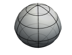
(a)  $n=1.7$

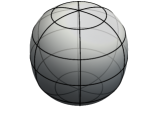
(b)  $n=2.5$

Figure 1: Supereggs for different exponents $n$.

III.2 Rounded cylinder and Stadium of revolution

Next, we consider a rounded cylindrical enclosure in three dimensions. If we consider a rounded rectangular region with circular arc of radius $R$ and the separation in between them of $d$ in a plane, then the surface of revolution around the major axis will be a rounded cylinder of height and base diameter equal to $2(d+R)$. The equation of the rounded rectangle in polar coordinate is

$${\mathcal{R}}(\theta)=\begin{cases}-\frac{d+R}{\sin\theta}&-\frac{\pi}{2}\leq\theta\leq-\tan^{-1}(\frac{d+R}{d})\\ -d(\sin\theta-\cos\theta)+\sqrt{\left(R^{2}-d^{2}\right)-2d^{2}\sin 2\theta}&-\tan^{-1}(\frac{d+R}{d})\leq\theta\leq-\tan^{-1}(\frac{d}{d+R})\\ \frac{d+R}{\cos\theta}&-\tan^{-1}(\frac{d}{d+R})\leq\theta\leq\tan^{-1}(\frac{d}{d+R})\\ d(\sin\theta+\cos\theta)+\sqrt{\left(R^{2}-d^{2}\right)+2d^{2}\sin 2\theta}&\tan^{-1}(\frac{d}{d+R})\leq\theta\leq\tan^{-1}(\frac{d+R}{d})\\ \frac{d+R}{\sin\theta}&\tan^{-1}(\frac{d+R}{d})\leq\theta\leq\frac{\pi}{2}\end{cases}$$ (26)

and the form of the rounded cylinder in spherical polar coordinate is

$$r(\theta,\phi)={\mathcal{R}}\left(\theta-\frac{\pi}{2}\right);\qquad\leavevmode\nobreak\ \text{for}\leavevmode\nobreak\ \leavevmode\nobreak\ \theta\in[0,\pi]\leavevmode\nobreak\ \leavevmode\nobreak\ \text{and}\leavevmode\nobreak\ \leavevmode\nobreak\ \phi\in[0,2\pi].$$ (27)

The shape of the rounded cylinder is displayed in fig (2a). Further, we consider the stadium of revolution in three dimensions. It is a surface of revolution attained by rotating a half stadium shape in two dimensions about its major axis. The equation of the half stadium in polar coordinate is

$${\mathcal{S}}(\theta)=\left\{\begin{array}[]{ll}-\frac{d}{2}\sin\theta+\sqrt{R^{2}-\left(\frac{d}{2}\cos\theta\right)^{2}}&\qquad-\frac{\pi}{2}\leq\theta\leq-\tan^{-1}(\frac{d}{2R})\\ \frac{R}{\cos\theta}&\qquad-\tan^{-1}(\frac{d}{2R})\leq\theta\leq\tan^{-1}(\frac{d}{2R})\\ \frac{d}{2}\sin\theta+\sqrt{R^{2}-\left(\frac{d}{2}\cos\theta\right)^{2}}&\qquad\tan^{-1}(\frac{d}{2R})\leq\theta\leq\frac{\pi}{2}\end{array}\right.$$ (31)

where $R$ is the radius of the circular arc and $d$ is the separation between them. The angular co-ordinate $\theta$ is in the usual sense. The form of stadium of revolution in three dimensions in spherical polar coordinate is simply given by

$$r(\theta,\phi)={\mathcal{S}}\left(\theta-\frac{\pi}{2}\right);\qquad\leavevmode\nobreak\ \text{for}\leavevmode\nobreak\ \leavevmode\nobreak\ \theta\in[0,\pi]\leavevmode\nobreak\ \leavevmode\nobreak\ \text{and}\leavevmode\nobreak\ \leavevmode\nobreak\ \phi\in[0,2\pi].$$ (32)

The shape of the stadium of revolution in three dimensions is depicted below in fig (2b).

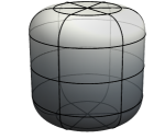
(a)  Rounded cylinder

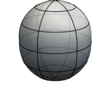
(b)  Stadium of revolution

Figure 2: The figure in the left (2a) is a rounded cylinder with the parameters $d=3\sqrt{3}/10$ and $R=2\sqrt{3}/10$ while the right one (2b) is the stadium of revolution with the parameters $d=1/4$ and $R=1$.

III.3 Spheroids

A spheroid in the spherical polar coordinates is given by

$$r(\theta,\phi)=\frac{r_{a}}{\sqrt{1-\left[1-\left(r_{a}/r_{c}\right)^{2}\right]\cos^{2}\theta}};\qquad\theta\in[0,\pi]\leavevmode\nobreak\ \leavevmode\nobreak\ \text{and}\leavevmode\nobreak\ \leavevmode\nobreak\ \phi\in[0,2\pi],$$ (33)

where $r_{a}$ and $r_{c}$ $(>0)$ are called equatorial and polar radii respectively. For $r_{c}<r_{a}$ the spheroid is known as oblate while for $r_{c}>r_{a}$ it is called prolate. We have considered $r_{c}/r_{a}=0.8$ for oblate and $r_{c}/r_{a}=1.2$ for prolate as case studies (since these two values are on the opposite sides of the sphere ($r_{c}=r_{a}=1$) and have considerable deformation from it) to show the applicability of the formalism. It is evident form (33) that an oblate fig (3a) (a prolate fig (3b)) is generated by rotating an ellipse about its minor (major) axis.

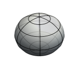
(a)  Oblate, $r_{c}/r_{a}=0.8$

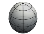
(b)  Prolate, $r_{c}/r_{a}=1.2$

Figure 3: Spheroids for different ratios of polar radius ($r_{c}$) to equatorial radius ($r_{a}$).

III.4 Pear shaped enclosures

Finally, we consider the following pear shaped domains motivated by the recent work [24] in the experimental nuclear physics for the ²²⁰Rn and ²²⁴Ra nuclei. The equation of the pear shape in spherical polar coordinate is given by

$$r(\theta,\phi)=R_{0}\left(1+\sum\limits_{a=2}^{4}C_{a}Y_{a}^{0}(\theta,\phi)\right);\qquad\leavevmode\nobreak\ \text{for}\leavevmode\nobreak\ \leavevmode\nobreak\ \theta\in[0,\pi]\leavevmode\nobreak\ \leavevmode\nobreak\ \text{and}\leavevmode\nobreak\ \leavevmode\nobreak\ \phi\in[0,2\pi],$$ (34)

where $R_{0}$ is the radius of equal volume spherical shape, which we set to one. The values for the expansion coefficients $C_{a}$s are identified with the parameter $\beta_{a}$s and chosen as the same given in [24, 27]. The shapes with these values are shown in fig (4).

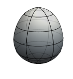
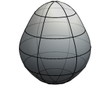
Figure 4: The pear shaped domains for different parameter values. The figures in the left and right are for the parameter values $\{C_{2},C_{3},C_{4}\}$ =$\{0.119,0.095,0.002\}$ and $\{0.154,0.097,0.080\}$ respectively.

IV Results and Discussions

These particular forms of $r(\theta,\phi)$, given in (25), (27), (32), (33) and (34), have been used to estimate the metric deformation in terms of the spherical harmonic expansion coefficients and those coefficients have been used for the calculation of eigenfunction corrections as well as energy corrections up to the second order of perturbation. The specific examples chosen here are motivated by physical problems and they possess axisymmetric property which is required for our formalism in the cases of degenerate states. The perturbative series converges quickly with the main contribution coming from the first few terms. It is clear that the convergence of the expansion coefficients will guarantee the convergence of the perturbative series for the energy as the $m^{\rm{th}}$ order corrections are $m$-linear in the expansion coefficients. The following figure (5) shows the convergence of the spherical harmonics expansion coefficients for the above mentioned shapes (for the pear shapes it is obvious from the deformation parameters given in fig (4)). The method seems to work quite well for the geometries having no sharp corners.

(a)  Superegg

(b)  Stadium of revolution

(c)  Spheroid

(d)  Rounded cylinder

Figure 5: This shows the convergence of the expansion coefficients ($C_{a}$) with the number of terms. In fig (5a) solid (dotted) lines indicate the coefficients for a superegg with exponent $n=1.7$ ($n=2.5$) and similarly, in fig (5c) for oblate (prolate). Figs (5b) and (5d) show the coefficients for a stadium of revolution and a rounded cylindrical enclosure respectively.

in this formalism, the only approximation introduced is due to the restriction of the perturbative series to the second order. In principle the higher order corrections could also be calculated exactly and the results could be improved further. As it is evident from the results that the third and higher order corrections would be meaningful only when one has violent deformations of a sphere and where the $C_{a}$s are not small and not converging rapidly. We have compared the eigenvalues obtained analytically by our method with the numerical ones for supereggs and a stadium of revolution together in table (1) and spheroids and a rounded cylinder in table (2) for both the cases of boundary conditions. In the case of DBC we have considered energy levels (including degenerate ones) up to the $17^{\rm{th}}$ state while for NBC those are up to the $16^{\rm{th}}$ state. The percentage deviations of the analytical values from the corresponding numerical ones are also shown. The results imply that this perturbative formalism works considerably well even for higher excited states and also for domains which are highly deformed. For this extreme cases addition of higher order corrections will surely improve the matching but they are algebraically complicated. Due to the deformation from the sphere the degenerate states, of multiplicities $(2l+1)$ for a given $l$ value, will be splitted. It is observed that for degenerate states the energy corrections are same for equal $|m|$ values and which implies that we get only $(l+1)$ distinct energy values. In case of a spherical boundary the energy levels having degeneracy $\{3\}$ or $\{5\}$ transformed after the deformation into $\{2,1\}/\{1,2\}$ or $\{1,2,2\}/\{2,2,1\}/\{2,1,2\}$-fold degeneracy respectively. Also the energy levels for different $l,m$ values are interlaced among each other after the deformation in a wild fashion for higher excited states and due to that we restrict the comparison only for low-lying levels. The matching between the analytical results and the corresponding numerical counterparts are excellent for the shapes which are not highly deformed and for non-trivial shapes also the agreement is quite satisfactory. In case of DBC, in table (1) the discrepancy is $<0.01\%$ for supereggs and stadium of revolution with a maximum of $\sim 0.7\%$ while for NBC it is relatively larger ($<0.1\%$) with a maximum of $\sim 0.2\%$ for the stadium. Next we have clubbed oblate, prolate and rounded cylinder domains together. Even though the magnitude of deviation from the sphere is same for the oblate and prolate considered here, the shapes are completely different and as a result the matching is also dissimilar. In table (2) the mismatch is $<1\%$ and maximum deviations for the oblate is $\sim 1.5\%$ and for the prolate it is mostly $<1.5\%$ and goes up to $\sim 4\%$ for couple of levels. For rounded cylinder the errors are within $\sim 1.7\%$. In case of NBC for the same group of boundaries the matching is very good (with errors are $\sim 1\%$ for spheroids and $<2\%$ for rounded cylinder) and the maximum discrepancies are $\sim 1.6\%$, $\sim 2.5\%$ and $\sim 3.9\%$ respectively for oblate, prolate and rounded cylinder enclosures for a few specific levels. Finally in the last table (3) we have compared the results for pear shaped domains satisfying both the DBC and the NBC with an analogy with the nuclear physics. The agreement between the analytic perturbative results and the numerical ones is better for the pear shape for which the $C_{a}$ values are small compared to other. The maximum deviation goes up to $2\%$ in the worst case for the DBC. While for the NBC it is evident from table (3) that the matching is excellent barring a couple of cases marked with stars ($\star$) and daggers ($\dagger$) (where it is disastrous) in that table. For these cases the mismatch is solely due to the accidental closeness of the zeros of derivative of spherical Bessel functions $j_{0}$ and $j_{3}$, which are $\alpha_{1,0}(=4.49341)$ and $\alpha_{1,3}(=4.51409)$ respectively. In the calculation of the second order energy correction for $l=0$ due to the non-zero finite value of $C_{3}$, the term of the form, $-\left(1+\frac{\alpha_{1,0}j_{3}(\alpha_{1,0})}{j^{\prime}_{3}(\alpha_{1,0})}\right)\frac{C^{2}_{3}}{2\pi}$, picks up a very high negative value (as the denominator is very close to zero) and causes the problem in the levels marked by stars ($\star$) for both the shapes. Similarly, for $l=3$ and $m=0$ the second order energy correction term, containing $\frac{\alpha_{1,3}j_{0}(\alpha_{1,3})}{j^{\prime}_{0}(\alpha_{1,3})}$, produces a large positive correction as the denominator is again very close to zero and which creates the error for the levels marked by daggers ($\dagger$) for both the cases. Other than the above mentioned exception the matching between the perturbative and numerical values are outstanding. The agreement between the numerical and perturbative values are better for supereggs than that for spheroids for both the cases of boundary conditions and is analogous to the behaviour of their two dimensional counterparts i.e. between supercircle and ellipse as reported in earlier works [28, 29]. We would like to point out that the eigenvalue correction for the state $l=2,m=0$ behaves in a peculiar fashion and disrupts the matching between different levels and produces the instances of maximum deviations for most of the cases in the above mentioned examples for both the boundary conditions. This abnormality for $l=2$ is an issue which calls for further investigations. Another unique feature of this method is that it can capture the degeneracy patterns for apparently similar looking shapes having different degeneracy patterns and also distinct shapes having similar type of degeneracies. As an example, the prolate, the stadium of revolution and the superegg ($n=2.5$) are looking similar apparently but the first two shapes have similar degeneracy pattern only for the DBC. The distinction is made in their NBC degeneracy patterns. In contrast, rounded cylinder and superegg ($n=2.5$) are having different structures but they produce similar degeneracy pattern for the DBC. So, our perturbative method traces the degeneracy patterns (provided by the numerical results) in a correct fashion for low-lying levels for different shapes and both the cases of boundary conditions. On the other hand, there are a few instances where three very close energylevels show degeneracy mismatch (viz. superegg ($n=1.7$) for DBC levels $5,6$ and $7$; oblate for NBC levels $13,14$ and $15$; rounded cylinder for NBC levels $11,12$ and $13$). We expect that inclusion of higher order correction term may provide a positive correction to the non-degenerate state whereas the two degenerate states may get a negative correction and which might bring them in order.

In conclusion, we point out that expansion of the boundary asymmetry in terms of spherical harmonics makes the method completely general to encompass a large variety of domains in three dimensions. The closed form corrections for wavefunctions and energies at each order of perturbation in terms of expansion coefficients help us to apply the prescription for a general boundary conditions also. Since the solutions are boundary condition free this method can tackle variety of problems. Also the boundary conditions maintain a simple form at each order of perturbation at the cost of complicating the equations. This method can treat both degenerate and non-degenerate states in the same way for axisymmetric boundaries. This method has an edge over the other method discussed by Panda and Hazra recently [8]. In the present method applying boundary condition is easy in contrast to the other method where it is extremely cumbersome. In this case all order equations as well as energy corrections are also written.

References

- [1] S. Panda, T. G. Sarkar, and S. P. Khastgir. Metric deformation and boundary value problems in 2d. Progress of Theoretical Physics, 127(1):57–70, 2012.
- [2] J. W. S. Rayleigh. The Theory of Sound. Dover Publications, New York, 1945. Vol 2, 2d ed.
- [3] P. M. Morse. Vibration and Sound. McGraw-Hill Kogakusha, Tokyo, 1948.
- [4] P. M. Morse and H. Feshbach. Methods of Theoretical Physics, Part I. McGraw-Hill, New York, 1953.
- [5] E. W. Weisstein. Superellipsoid (MathWorld A Wolfram Web Resource). http://mathworld.wolfram.com/Superellipsoid.html. Accessed: 22/07/2013.
- [6] I. Sobchenko, J. Pesicka, D. Baither, R. Reichelt, and E. Nembach. Superellipsoids: A unified analytical description of the geometry of nanoscale second-phase particles of any shape. Applied Physics Letters, 89(13):133107, 2006.
- [7] L. Gong, S. D. Pathak, D. R. Haynor, P. S. Cho, and Y. Kim. Parametric shape modeling using deformable superellipses for prostate segmentation. IEEE Trans. Med. Imaging, 23(3):340–349, 2004.
- [8] S. Panda and G. Hazra. Boundary perturbations and the Helmholtz equation in three dimensions. ArXiv e-prints, December 2012.
- [9] S. A. Moszkowski. Particle states in spheroidal nuclei. Phys. Rev., 99:803–809, Aug 1955.
- [10] T. Prosen. Quantization of a generic chaotic 3D billiard with smooth boundary. I. Energy level statistics. Physics Letters A, 233:323–331, February 1997.
- [11] T. Prosen. Quantization of generic chaotic 3D billiard with smooth boundary. II. Structure of high-lying eigenstates. Physics Letters A, 233:332–342, February 1997.
- [12] H. Primack and U. Smilansky. The quantum three-dimensional sinai billiard - a semiclassical anlaysis. Physics Reports, 327:1–107, March 2000.
- [13] T. Papenbrock. Numerical study of a three-dimensional generalized stadium billiard. Physical Review E, 61:4626–4628, April 2000.
- [14] I. M. Erhan and H. Taseli. A model for the computation of quantum billiards with arbitrary shapes. Journal of Computational and Applied Mathematics, 194:227–244, October 2006.
- [15] H. Alt, C. Dembowski, H. D. Gräf, R. Hofferbert, H. Rehfeld, A. Richter, R. Schuhmann, and T. Weiland. Wave dynamical chaos in a superconducting three-dimensional sinai billiard. Phys. Rev. Lett., 79:1026–1029, Aug 1997.
- [16] J. U. Nöckel and A. D. Stone. Ray and wave chaos in asymmetric resonant optical cavities. Nature, 385(6611):45–47, 1997.
- [17] P. L. Arlett, A. K. Bahrani, and O. C. Zienkiewicz. Application of finite elements to the solution of helmholtz's equation. Proceedings of the Institution of Electrical Engineers, 115(12):1762–1766, 1968.
- [18] P. K. Banerjee, P. K. Banerjee, and R. Butterfield. Boundary element methods in engineering science. McGraw-Hill Book Co. (UK), 1981.
- [19] J. T. Chen, M. H. Chang, K. H. Chen, and I. L. Chen. Boundary collocation method for acoustic eigenanalysis of three-dimensional cavities using radial basis function. Computational Mechanics, 29(4-5):392–408, 2002.
- [20] E. Larsson and B. Fornberg. A numerical study of some radial basis function based solution methods for elliptic pdes. Computers and Mathematics with Applications, 46(56):891–902, 2003.
- [21] L. Fox, P. Henrici, and C. Moler. Approximations and bounds for eigenvalues of elliptic operators. SIAM Journal on Numerical Analysis, 4(1):pp. 89–102, 1967.
- [22] A. Bogomolny. Fundamental solutions method for elliptic boundary value problems. SIAM Journal on Numerical Analysis, 22(4):644–669, 1985.
- [23] Here we have used an unusual notation for zeros of spherical Bessel functions and their derivatives. Conventionally, and denote zeros of and respectively.
- [24] L. P. Gaffney et al. Studies of pear-shaped nuclei using accelerated radioactive beams. Nature (London), 497:199–204, May 2013.
- [25] E. W. Weisstein. Superegg (MathWorld A Wolfram Web Resource). http://mathworld.wolfram.com/Superegg.html. Accessed: 22/07/2013.
- [26] M. Gardner. Mathematical carnival : a new round-up of tantalizers and puzzles from Scientific American. Vintage Books, New York, 1977.
- [27] W. Nazarewicz, P. Olanders, I. Ragnarsson, J. Dudek, G.A. Leander, P. Möller, and E. Ruchowsa. Analysis of octupole instability in medium-mass and heavy nuclei. Nuclear Physics A, 429(2):269 – 295, 1984.
- [28] S. Chakraborty, J. K. Bhattacharjee, and S. P. Khastgir. An eigenvalue problem in two dimensions for an irregular boundary. Journal of Physics A: Mathematical and General, 42(19):195301–+, May 2009.
- [29] S. Panda, S. Chakraborty, and S. P. Khastgir. Eigenvalue problem in two dimensions for an irregular boundary: Neumann condition. The European Physical Journal Plus, 126:1–20, 2011. 10.1140/epjp/i2011-11062-4.