Phase transitions in 2D $J_{1}-J_{2}$ model with arbitrary signs of exchange interactions

Abstract

The ground state of the $S=1/2$ $J_{1}-J_{1}$ Heisenberg model on the 2D square lattice with arbitrary signs of exchange constants is considered. States with different spin long-range order types (antiferromagnetic checkerboard, stripe, collinear ferromagnetic) as well as disordered spin-liquid states are described in the frames of one and the same analytical approach. It is shown inter alia, that the phase transition between ferromagnetic spin liquid and long-range order ferromagnet is a second-order one. On the ordered side of  the transition the ferromagnetic state with rapidly varying condensate function is detected.

Investigation of the two-dimensional frustrated Heisenberg model is of current importance for understanding magnetic properties of various layered compounds. Spin subsystem of $CuO_{2}$ planes in cuprate high-temperature superconductors (HTSC) can be described by $J_{1}-J_{2}$ Heisenberg model on the square lattice with spin $S=1/2$ and antiferromagnetic signs of both exchange constants. Intensively studied layered vanadium oxides can be described in the frames of same model, but not only with antiferromagnetic exchanges.

In the classical limit $S\gg 1$ at zero temperature three types of long-range order (LRO) are realized: ferromagnetic (FM), Neel antiferromagnetic (AFM) and columnar (stripe). At the points $J_{2}/\left|J_{1}\right|=0.5$ there are first order phase transitions from checkerboard AFM order to stripe for $J_{1}>0$ and from stripe to ferromagnetic order for $J_{1}<0$, at point $J_{1}=0$, $J_{2}=-1$ there is a transition from AFM to FM order. The positions of the better-studied vanadates on the classical $J_{1}$–$J_{2}$ model phase diagram are shown in Fig. 1 (the data from Refs. Nath08, ; Tsirlin09, ).

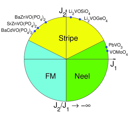
Figure 1: Phase diagram of the $J_{1}$–$J_{2}$ Heisenberg model on the 2D square lattice in the classical limit. Dots represent the relations between $J_{1}$ and $J_{2}$ for the better-studied vanadates (data from Nath08 ; Tsirlin09 ).

At $T\neq 0$ long-range order due to Mermin-Wagner theorem is impossible for any spin, at $T=0$ for large $S$ LRO exists throughout the ”$J_{1}-J_{2}$-circle”. Nevertheless, it is generally accepted that for $S=1/2$ even for $T=0$ spin fluctuations near phase transition points lead the system to one of the singlet states without LRO and with nonzero spin gap. The structure of disordered phases remains debatable. Usually the following states are considered: spin liquid, conserving translational and $SU(2)$ symmetry of the Hamiltonian; plaquette lattice covering, which breaks translational symmetry, but conserves $SU(2)$ symmetry; and states that break both translational and $SU(2)$ symmetry.

In the present work the ground state of 2D $J_{1}-J_{2}$ Heisenberg model is investigated in the frames of spherically symmetric self-consistent approach (SSSA) for two-time retarded Green’s functions (Refs. Shimahara91, ; BarBer94-both, , see also recent review in Ref. BarMixTMF11, ). This approach automatically conserves $SU(2)$ symmetry of the Hamiltonian, translational symmetry and spin constraint on the site. Unlike previous treatments of $S=1/2$ model, we investigate the entire phase diagram for arbitrary values of $J_{1}$ and $J_{2}$, including cases of $J_{1}<0$, $J_{2}>0$ and $J_{1}<0$, $J_{2}<0$.

In the quantum limit $S=1/2$, the first quadrant of the diagram $0\leq\varphi\leq\pi/2$, $\tan\varphi=J_{2}/J_{1}$, $J_{1},\ J_{2}>0$, has been studied up to now most extensively. In this case a disordered state (spin liquid) appears between AFM and stripe LRO phases. The transitions AFM — spin liquid — stripe phase are continuous in the frames of SSSA.

The region $J_{1}<0$, $J_{2}>0$ for $S=1/2$ of the phase diagram has been investigated in frames of SSSA in Hartel11 ; Hartel13 , where the the first order transition between FM LRO state and spin liquid has been stated. As it will be seen hereafter, unlike Hartel11 ; Hartel13 , our consideration leads a continuous second-order transition between the mentioned states, the properties of FM state being significantly modified near the transition.

Before discussing the phase diagram in the whole range of the angle $\varphi$, let us write down the Hamiltonian $H$ and the form of spin-spin Green’s function $G^{zz}\left(\omega,\mathbf{q}\right)$, which can be obtained in the frames of SSSA Shimahara91 ; BarBer94-both ; BarMixTMF11 ; Hartel11 ; Hartel13 (for SSSA $G^{zz}=G^{xx}=G^{yy}$; $\langle S_{\mathbf{i}}^{\alpha}\rangle=0,$ $\alpha=x,y,z$).

$$H=\frac{J_{1}}{2}\sum_{\mathbf{i},\mathbf{g}}\widehat{\mathbf{S}}_{\mathbf{i}}\widehat{\mathbf{S}}_{\mathbf{i}+\mathbf{g}}+\frac{J_{2}}{2}\sum_{\mathbf{i},\mathbf{d}}\widehat{\mathbf{S}}_{\mathbf{i}}\widehat{\mathbf{S}}_{\mathbf{i}+\mathbf{d}}$$ (1)

$$G^{zz}\left(\omega,\mathbf{q}\right)=\langle S_{\mathbf{q}}^{z}|S_{-\mathbf{q}}^{z}\rangle_{\omega}=\frac{F_{\mathbf{q}}}{\omega^{2}-\omega_{\mathbf{q}}^{2}}$$ (2)

$$F_{\mathbf{q}}=-8[J_{1}(1-\gamma_{g})c_{g}+J_{2}(1-\gamma_{d})c_{d}]$$ (3)

$$\gamma_{g}(\mathbf{q})=\frac{1}{z_{g}}\sum_{\mathbf{g}}e^{i\mathbf{qg}}=\frac{1}{2}(\cos(q_{x})+\cos(q_{y}))$$ (4)

$$\gamma_{d}(\mathbf{q})=\frac{1}{z_{d}}\sum_{\mathbf{d}}e^{i\mathbf{qd}}=\cos(q_{x})\cos(q_{y})$$ (5)

where $\mathbf{g},\ \mathbf{d}$ are vectors of nearest and next-nearest neighbors, $c_{R}=\langle S_{\mathbf{n}}^{z}S_{\mathbf{n+R}}^{z}\rangle$ — spin-spin correlation functions on the corresponding coordination spheres, $z_{g}=z_{d}=4$ — number of sites on the first and the second coordination spheres. Hereafter all the energetical parameters are set in the units of $J=\sqrt{J_{1}^{2}+J_{2}^{2}}$.

For further analysis, it is convenient to represent the spin excitation spectrum $\omega_{\mathbf{q}}^{2}$ (BarBer94-both ; BarMixTMF11 ) in three following forms:

$$\omega_{\mathbf{q}}^{2} = 2A\left(\mathbf{q}\right)\left(1-\gamma_{g}\right)\left(1-\gamma_{g}+\delta_{FM}\left(\mathbf{q}\right)\right)=$$ (6)

$$= -2A\left(\mathbf{q}\right)\left(1-\gamma_{g}\right)\left(1+\gamma_{g}+\delta_{AFM}\left(\mathbf{q}\right)\right)=$$

$$= -2A\left(\mathbf{q}\right)\left(1-\gamma_{g}\right)\left(1+\gamma_{d}+\delta_{Stripe}\left(\mathbf{q}\right)\right)$$

Expressions for $A$ and $\delta$ from (6) are rather unwieldy, and we do not present them completely. We will just present the form of $A\delta_{AFM}$ as an example:

$$A\,\delta_{FM}=8J_{1}J_{2}\left(\widetilde{c}_{dg}\!-\!\widetilde{c}_{g}\right)+\!J_{1}^{2}\left(1\!-\!20\widetilde{c}_{g}\!+\!8\widetilde{c}_{d}\!+\!4\widetilde{c}_{2g}\right)+$$

$$+\frac{1\!-\!\gamma_{d}}{1\!-\!\gamma_{g}}[8J_{2}J_{1}\left(\widetilde{c}_{dg}\!-\!\widetilde{c}_{g}\right)+\!J_{2}^{2}\left(1\!-\!20\widetilde{c}_{d}\!+\!8\widetilde{c}_{2g}\!+\!4\widetilde{c}_{2d}\right)]$$ (7)

In (7) the correlators $\widetilde{c}_{r}=\alpha c_{r}$ are written in one vertex $\alpha$ approximation (BarMixTMF11 ; Hartel11 ). Five correlators $c_{r}$ ($r=g,\ d,\ 2g,\ r_{gd}=|\mathbf{g}+\mathbf{d}|,\ 2d$) and vertex correction $\alpha$ are obtained self-consistently through the Green’s function $G^{zz}$. The additional condition is the exact sum rule fulfillment $\langle\widehat{\mathbf{S}}_{\mathbf{i}}^{2}\rangle=3/4$.

The introduced parameters $\delta_{FM}\left(\mathbf{q}\right)$, $\delta_{AFM}\left(\mathbf{q}\right)$, and $\delta_{Stripe}\left(\mathbf{q}\right)$ have a clear physical meaning and define the spin excitation spectrum basic properties. For all phases — three ordered (AFM, stripe, and FM), and spin liquid — the spin gap is closed at the zero point $\mathbf{\Gamma}=\left(0,0\right)$. In the FM phase the spectrum around $\mathbf{\Gamma}$ is quadratic in $q$, for other phases it is linear. Near the transitions to FM from the neighboring phases the spectrum around $\mathbf{\Gamma}$ has the form $\omega_{q}\sim q\sqrt{\delta_{FM}+\frac{q^{2}}{4}}$. So $\delta_{FM}$ dictates the conversion from FM spectrum $\omega_{q}\sim q^{2}$ to $\omega_{q}\sim q$. In the AFM phase the spin gap is closed not only in $\mathbf{\Gamma}$, but also in AFM point $\mathbf{Q}=\left(\pi,\pi\right)$. When approaching to the AFM phase from the neighboring phases the spectrum around $\mathbf{Q}$ is $\omega_{q}\sim\sqrt{\delta_{AFM}+\varkappa^{2}}$, $\varkappa=|\mathbf{Q-q}|$, i.e. $\delta_{AFM}$ directly defines the gap $\Delta_{AFM}$ in the spectrum. For the stripe phase and it’s neighborhood the situation is similar to that for AFM phase (with corresponding substitutions, the role of control point goes from $\mathbf{Q}$ to to stripe points $\mathbf{X}=(0,\pi),(\pi,0)$).

Thus, vanishing of any of the three parameters $\delta_{FM}$, $\delta_{AFM}$, $\delta_{Stripe}$ defines transition to the corresponding ordered phase and simultaneous alteration of the spectrum near the corresponding control point (transition from linear to quadratic for FM and vanishing of the spin gap in the Dirac spectrum for two others). For the spin liquid the spectrum gap is opened in the whole Brillouin zone except $\mathbf{\Gamma}$.

Let us depict in more detail the description of the spin LRO. The structure factor has the form

$$c_{\mathbf{q}} = \langle S_{\mathbf{q}}^{z}S_{-\mathbf{q}}^{z}\rangle=-\frac{1}{\pi}\int d\omega\,n\left(\omega_{\mathbf{q}}\right)\mathrm{Im}G^{zz}\left(\omega,\mathbf{q}\right)=$$ (8)

$$= \frac{F_{\mathbf{q}}}{2\omega_{\mathbf{q}}}\left(2n\left(\omega_{\mathbf{q}}\right)+1\right)$$

here $n\left(\omega_{\mathbf{q}}\right)$ is Bose function. Correlation functions are expressed through the structure factor as

$$c_{R} = \langle S_{\mathbf{n}}^{z}S_{\mathbf{n+R}}^{z}\rangle=\sum_{\mathbf{q}}c_{\mathbf{q}}e^{i\mathbf{qR}}=$$ (9)

$$= c_{cond}\sum_{\mathbf{q}_{0}}e^{i\mathbf{q}_{0}\mathbf{R}}+\frac{1}{4\pi^{2}}\int d\mathbf{q}e^{i\mathbf{qR}}\frac{F_{\mathbf{q}}}{2\omega_{\mathbf{q}}}$$

where the condensate part is

$$c_{cond}=\lim_{T\rightarrow 0}\frac{1}{4\pi^{2}}\int d\mathbf{q}n\left(\omega_{\mathbf{q}}\right)\frac{F_{\mathbf{q}}}{\omega_{\mathbf{q}}}$$ (10)

At $T\rightarrow 0$ $\delta$-like peaks in the structure factor can appear at some points $\mathbf{q}_{0}$ of the Brillouin zone (where $\omega_{\mathbf{q}}$ tends to zero), this peaks being induced by the Bose function $n\left(\omega_{\mathbf{q}}\right)$. Then the condensate term $c_{cond}$ appears in the correlation functions $c_{R}$. This corresponds to the LRO existence ($c_{cond}$ defines spin-spin correlator at the infinity). The term without $n\left(\omega_{\mathbf{q}}\right)$ on the right hand side of (9) goes to zero as $R\rightarrow\infty$.

For AFM and stripe long-range orders the condensate term appears as the spectrum $\omega_{\mathbf{q}}$ vanishes correspondingly at the points $\mathbf{Q}$ and $\mathbf{X}$. As mentioned above, the spectrum near this points is (in the corresponding phase) $\omega_{\mathbf{q}}\sim\varkappa$, where $\varkappa=\left|\mathbf{q}-\mathbf{Q}\right|$ or $\left|\mathbf{q}-\mathbf{X}\right|$. The Green’s function numerator $F_{\mathbf{q}}$ does not vanish at this points. The spectrum linearity and nonzero $F_{\mathbf{q}}$ value constitute the condition for condensate to appear Shimahara91 .

In the presence of FM LRO spin condensate appears at the point $\mathbf{\Gamma}$. Near this point the Green’s function numerator $F_{\mathbf{q}}\sim q^{2}$, so the spectrum near $\mathbf{\Gamma}$ is to be also quadratic $\omega_{\mathbf{q}}\sim q^{2}$ for the condensate to appear.

Note that if the third exchange interaction $J_{3}$ is added to the model, the helical LRO can also be realized. In the $J_{1}-J_{2}-J_{3}$ model the condensate peak point in the structure factor can be located not only at $\mathbf{\Gamma}$, $\mathbf{Q}$, or $\mathbf{X}$, but also at arbitrary incommensurate point on the side or diagonal of the Brillouin zone MixBarJETPL11 .

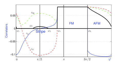
Figure 2: The condensate $c_{cond}$ (absolute value of spin-spin correlator at infinity) and spin-spin correlators on the first three coordination spheres dependence on $\varphi$ ($J_{1}=\cos\varphi,$ $J_{2}=\sin\varphi$). Black bold line shows $c_{cond}$, blue solid line — $c_{g}$, red dotted — $c_{d}$, green dash dotted — $c_{2g}$. The points of phase transitions are marked on the x-axis: $\varphi_{1}$ – AFM $\rightarrow$ SL¹ transition, $\varphi_{2}$ — SL¹ $\rightarrow$ Stripe, $\varphi_{3}$ — Stripe $\rightarrow$ SL², $\varphi_{4}$ — SL² $\rightarrow$ FM¹ (for the rescaled vicinity of $\varphi_{4}$ see Fig.4), $\varphi_{6}$ — FM² $\rightarrow$ AFM transition. See text for details.

Fig. 2 shows the phase diagram at $T\rightarrow 0$, the condensates and correlators corresponding to first three coordination spheres being depicted. Fig. 3 represents spin gaps in the symmetrical points. In the interval $0\leq\varphi\leq\varphi_{1}=0.051$ AFM LRO is realized: spin gap at AFM point $\mathbf{Q}$ is zero, $\Delta_{\mathbf{Q}}=0$, the spectrum near $\mathbf{Q}$ is linear in $|\mathbf{q}-\mathbf{Q}|$, there is a nonzero AFM condensate $c_{cond}^{AFM}$.

At $\varphi=\varphi_{1}$ condensate $c_{cond}^{AFM}$ vanishes, AFM gap $\Delta_{\mathbf{Q}}$ opens, and the spectrum becomes ungapped in the whole Brillouine zone, except trivial zero point $\mathbf{\Gamma}$, where it remains linear. The system turns to spin liquid state (let’s denote it by SL¹), which is realized in the interval $\varphi_{1}\leq\varphi\leq\varphi_{2}=1.111$. In this phase LRO is absent, and short-range order transforms with growing $\varphi$ from the AFM-like ($c_{g}<0$, $|c_{g}|>c_{d}>c_{2g}>0$) to the one typical for stripe phase ($c_{d}<0,$ $c_{2g}>0$, $|c_{d}|>c_{2g}>|c_{g}|$). At the same time spin gap at the point $\mathbf{Q}$ passes through the maximum, and the gap at stripe points $\mathbf{X}$ monotonically decreases (Fig. 3).

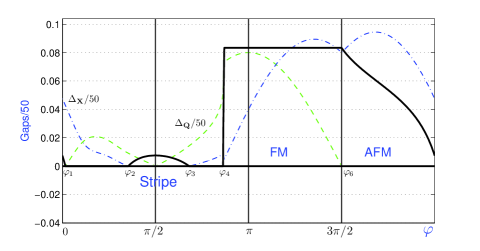
Figure 3: Spin gaps $\Delta_{\mathbf{Q}}$ and $\Delta_{\mathbf{X}}$ ($\Delta_{\mathbf{Q}}$/50 and $\Delta_{\mathbf{X}}$/50 are shown) at the points $\mathbf{Q}=(\pi,\pi)$ (green dashed line) and $\mathbf{X}=(0,\pi),(\pi,0)$ (blue dash-dotted) of the Brillouin zone as functions of $\varphi$ ($J_{1}=\cos\varphi,$ $J_{2}=\sin\varphi$). Black solid line — condensate $c_{cond}$. All the points $\varphi_{1}$–$\varphi_{6}$ are the same as in Fig.2.

At $\varphi=\varphi_{2}$ the stripe gap $\Delta_{\mathbf{X}}$ vanishes, the spectrum at stripe points $\mathbf{X}$ becomes linear, and condensate $c_{cond}^{Stripe}$ becomes nonzero, the system turns to the LRO stripe phase, which is realized in the interval $\varphi_{2}\leq\varphi\leq\varphi_{3}=2.141$. Note the very interesting point $\varphi=\pi/2$, where $J_{1}=0$, $J_{2}=1$. The lattice with this exchange couplings splits into two noninteracting AFM sublattices. Then it is obvious that $c_{d}\left(\pi/2\right)=c_{g}\left(0\right)$, $c_{2g}\left(\pi/2\right)=c_{d}\left(0\right)$ (see Fig. 2). Note that at $\varphi=\pi/2$, as in AFM phase, $\Delta_{\mathbf{Q}}=0$ (see Fig. 3), however, this does not lead to AFM LRO, because $F\left(\mathbf{Q},\varphi=\pi/2\right)$ also vanishes, and as a result $c_{cond}^{AFM}\left(\varphi=\pi/2\right)=0$.

At the point $\varphi=\varphi_{3}$ stripe gap $\Delta_{\mathbf{X}}$ opens, and the system again turns to the spin liquid state (SL²), realized in the interval $\varphi_{3}<\varphi<\varphi_{4}=2.712$ (but the structure of the short-range order differs from that at $\varphi_{1}\leq\varphi\leq\varphi_{2}$). It is worth noting, that the next-nearest neighbor correlator $c_{d}$ remains negative throughout the SL² existence, i.e. the short-range order is not rearranged to the FM-like, where $c_{g},c_{d},c_{2g}>0$. The absolute value of $c_{d}$ almost everywhere, except tiny region near $\varphi_{4}$, is larger than the nearest neighbor correlator $c_{g}$.

Let us emphasize ones more, that for all the mentioned phases the spectrum near $\mathbf{\Gamma}=(0,0)$ is linear in $q$.

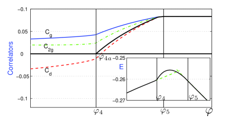
Figure 4: Condensate $c_{cond}$ and correlators $c_{g}$, $c_{d}$, $c_{2g}$ evolution from spin liquid SL² to ferromagnetic state FM². As in Fig.2, black bold line — $c_{cond}$, blue solid — $c_{g}$, red dotted — $c_{d}$, green dash dotted — $c_{2g}$. $\varphi_{4}$ corresponds to the transition from spin liquid $SL^{2}$ to ferromagnetic state FM¹, in the narrow region $\varphi_{4}$–$\varphi_{4a}$ short-range FM order is absent, while long-range FM order is present (see text), $\varphi_{5}$ — the border between ferromagnetic regions FM¹ and FM² (see text).
Inset: black solid line — energy per site $\varepsilon$ of the present work, green dashed lines — energy extrapolation for the solutions SL² and FM² from Ref. Hartel11, . The intersection corresponds to first-order transition between spin liquid and ferromagnet, stated in Hartel11 .

At $\varphi=\varphi_{4}$ there again appears a phase with LRO (ferromagnetic) and nonzero corresponding condensate $c_{cond}^{FM}$. Spectrum near the point $\mathbf{\Gamma}$ becomes quadratic in $q$ (and the gap $\Delta_{\mathbf{\Gamma}}(\varphi_{4})=0$). Fig. 2 and Fig. 3 demonstrate, that two regions are distinguishable in this phase — FM¹ and FM². FM¹ covers in the tiny interval $\varphi_{4}<\varphi<\varphi_{5}=2.733$. Here condensate $c_{cond}^{FM}$ grows rapidly with the increase of $\varphi$ from $c_{cond}^{FM}=0$ to the maximal value $c_{cond}^{FM}=1/12$. Note, that near $\varphi_{4}$ FM LRO without FM short-range order is realized, $c_{d}<0$ (the corresponding interval is $\varphi_{4}<\varphi<\varphi_{4a}=2.713$). For $\varphi\geq\varphi_{5}$ (FM² region) all the correlators and the condensate are equal to $1/12$ and the vertex correction $\alpha=3/2$ Shimahara91 ; Hartel11 ).

FM¹ region was not detected (Fig. 4) in Hartel11 . The inset of Fig. 4 shows the energy at the transitions SL² $\rightarrow$ FM¹ $\rightarrow$ FM². Dashed line is the extrapolatin of SL² energy to the intersection with the FM² energy (from Hartel11 ). Based on this extrapolation, it was concluded in Hartel11 , that a first order transition occurs near the intersection point. Our consideration leads to a conclusion (see Fig. 4), that the energy derivative is continuous between SL² and FM¹.

Note that standard FM² solution Shimahara91 ; Hartel11 exists also for angles $\varphi<\varphi_{5}$, down to $\varphi=\pi-\arctan\left(1/2\right)$, but in this region it happens to be metastable relative to FM¹ and SL².

At the angles $\varphi\geq\varphi_{5}$ the FM² solution is realized up to $\varphi_{6}=3\pi/2$. This point is a very special one. At $\varphi_{6}$ the lattice is splitted into two noninteracting sublattices. At $\varphi\rightarrow\varphi_{6}-0$ there is no frustration with respect to the FM order, at $\varphi\rightarrow\varphi_{6}+0$ — no frustration with respect to the AFM order. Therefore it is physically obvious that in the quantum limit a transition between these two phases is of the first order, as do our calculations confirm. Let us also note that, as it can be seen from Fig. 3, at $\varphi\rightarrow\varphi_{6}+0$ ($J_{1}=+0$, $J_{2}=-1$), AFM condensate, i.e. absolute value of the spin-spin correlation function at infinity, is much larger than in the ”standard” AFM ($\varphi=0$, $J_{1}=1$, $J_{2}=0)$, and is equal to FM condensate at $\varphi\rightarrow\varphi_{6}-0$. It means that FM next-nearest neighbor exchange with zero nearest exchange leads to stronger AFM order, than nearest AFM exchange with zero next-nearest one.

Figure 5: Dependence of spin liquid SL¹ borders position on the damping parameter $\gamma$ (see text for details).

In conclusion let us note, that the significant spin excitations damping can be expected near the transitions spin liquid $\rightarrow$ LRO phase. Accounting for the damping can shift the boundary of the corresponding transition. This is demonstrated in Fig. 5, where the dependence of SL¹ phase boundaries on the damping parameter $\gamma$ is represented. We used the simple semiphenomenological approximation for the Green’s function $G_{\gamma}^{zz}$, conserving correct analytical properties (see BarMixTMF11 for details).

$$G_{\gamma}^{zz}\left(\omega,\mathbf{q}\right)=\frac{F_{\mathbf{q}}}{\omega^{2}-\omega_{\mathbf{q}}^{2}+i\omega\gamma}$$ (11)

It can be seen in Fig. 5, that the SL phase boundaries are sensitive to the value of damping. Nethertheless, our estimates show, that there are no topological modifications of the phase diagram for any reasonable values of damping.

To summarize, in the present work the entire phase diagram of the 2D $J_{1}-J_{2}$ $S=1/2$ Heisenberg model is considered in the frames of one and the same approach. It is shown, that the transitions between all ordered and disordered phases are continuous, except the transition FM$\rightarrow$AFM at $J_{1}=0$, $J_{2}=-1$.

This work is supported by Russian Foundation for Basic Research, grant 13-02-00909a.

References

(1) R. Nath, A. A. Tsirlin, H. Rosner, and C. Geibel,
Phys. Rev. B78, 064422 (2008).
(2) A. A. Tsirlin and H. Rosner, Phys. Rev. B79,
214417 (2009).
(3) H. Shimahara and S. Takada, J. Phys. Soc. Jpn. 60, 2394 (1991).
(4) A. F. Barabanov and V. M. Berezovsky, JETP 79, 627 (1994); J. Phys. Soc. Jpn. 63, 3974 (1994).
(5) A. F. Barabanov, A. V. Mikheenkov, and A. V.
Shvartsberg, Theor. Math. Phys. 168, 1192 (2011).
(6) M. Hartel, J. Richter, D. Ihle, and S.-L. Drechsler,
Phys. Rev. B84, 104411 (2011).
(7) M. Hartel, J. Richter, O. Gotze, D. Ihle, and S.-L.
Drechsler, Phys. Rev. B87, 054412 (2013).
(8) A. V. Mikheyenkov, A. V. Shvartsberg, N. A.
Kozlov, and A. F. Barabanov, JETP Lett. 93, 377 (2011).