Geometrical crossover in two-body systems in a magnetic field

Abstract

An algebraic approach is formulated in the harmonic approximation to describe a dynamics of two-fermion systems, confined in three-dimensional axially symmetric parabolic potential, in an external magnetic field. The fermion interaction is considered in the form $\mbox{\rsfs U}_{M}(r)=\alpha_{M}\,r^{-M}$ $(\alpha_{M}>0,M>0)$. The formalism of a semisimple Lie group is applied to analyse symmetries of the considered system. Explicit algebraic expressions are derived in terms of system’s parameters and the magnetic field strength to trace the evolution of the equilibrium shape. It is predicted that the interplay of classical and quantum correlations may lead to a quantum shape transition from a lateral to a vertical localization of fermions in the confined system. The analytical results demonstrate a good agreement with numerical results for two-electron quantum dots in the magnetic field, when classical correlations dominate in the dynamics.

I Introduction

Symmetry breaking phenomena play important role in the interpretation of various physical properties of finite many-body systems, for example, such as nuclei cej and metallic grains kres . There exists a type of symmetry transformation that is specific for finite systems. This is a shape symmetry breaking, when a finite system, under varying external or internal parameters, exhibits the change of its shape. This change can be spontaneous, in the sense that the shape form is not imposed from outside, but the system acquires the chosen form because it is energetically profitable. Evidently, due to finite number of particles quantum fluctuations play essential role in the evolution of various properties of a system.

Recent progress in nanotechnology opens a broad avenue to study the interplay between microscopic (quantum) and macroscopic (classical) scales in mesoscopic systems. If in a mesoscopic system several particles are confined by a one-body field, the dynamics of the one-body field governs the individual motion of the particles. A natural question is how this is changed if the particles are influenced by a two-body interaction in addition to the one-body field. How, for example, in a mesoscopic system with a few particles moving in one-body potential could be exhibited a symmetry breaking phenomenon due to two-body interaction, related to a shape transition driven by quantum fluctuations ? The answer on this question may shed light on the connection between a shape transition and a quantum phase transition Sad in finite many-body quantum systems, in general.

To study the combined role of one-body and two-body interactions on symmetry breaking phenomena, we shall concentrate on the simplest nontrivial case, namely, the interacting two-body system. Specifically, we focus on two identical charged particles (electrons) in a three-dimensional deformed harmonic oscillator potential under a perpendicular magnetic field (see, for example, kai ; taut ; din ; ent ). It is noteworthy on the fact that semiconductor technology made possible to fabricate and probe such confined system at different values of the magnetic field as ; kou . Consequently, it has stimulated numerous theoretical studies on two-electron quantum dots (QDs), so-called ”artificial He atoms” (see for a recent review RM ; naz ; PR ). For example, a circular dot at arbitrary values of the magnetic field was studied in various approaches in order to find a closed-form solution loz ; kand1 ; grokr . Being a simplest nontrivial system, QD He poses a significant challenge to theorists. Indeed, using a two-dimensional He QD model, one is able to reproduce a general trend for the first singlet-triplet (ST) transitions observed in two-electron QDs under a perpendicular magnetic field. However, the experimental positions of the ST transition points are systematically higher kou ; nishi . The ignorance of the third dimension is the most evident source of the disagreement, especially, in vertical QDs din ; ron ; bruce ; nen3 .

The purpose of the present paper is to analyse correlation effects produced by a two-body interaction in most general form $\mbox{\rsfs U}_{M}(r)=\alpha_{M}\,r^{-M}$ $(\alpha_{M}>0,M>0)$ on the evolution of the ground and excited states of two-fermion (two-electron) systems under a perpendicular magnetic field. Although accurate numerical results for such potentials can be obtained readily, analytical results are still sought even in this case, because they provide the physical insight into numerical calculations. Moreover, analytical results could establish a theoretical framework for accurate analysis of confined many-electron systems, where the exact treatment of a three-dimensional (3D) case becomes computationally intractable.

The content of the paper is following. In Sec.II we formulate a general two-body problem confined by a one-body potential. Specifically, we consider two identical charged particles (electrons) in the field of the three-dimensional harmonic oscillator, interacting via a two-body interaction $\mbox{\rsfs U}_{M}(r)=\alpha_{M}\,r^{-M}$ $(\alpha_{M}>0,M>0)$. We show how the two-body Hamiltonian can be scaled, thus reducing the number of independent variables in the problem. This scale is related to an additional symmetry of the Hamiltonian function ($G_{4}$ group). Sec.III is devoted to the development of the algebraic approach to study shape transitions induced by the classical component of the total energy of two-electron system in a magnetic field. The role of quantum fluctuations is discussed in Sec.IV. The comparison of the analytical results with numerical calculations nen3 is presented Sec.V. Sec.VI summarizes briefly the main results. In Appendix some technical details of Sec.III are discussed.

II Model

We consider the Hamiltonian

$$H=\sum_{j=1}^{2}\bigg{[}\frac{1}{2m^{*}\!}\,\Big{(}{\bf p}_{j}-e\,{\mathsf{A}}_{j}\Big{)}^{\!2}+U({\mathsf{r}}_{j})\bigg{]}+\mbox{\rsfs U}_{M}({\mathsf{r}})+H_{\rm spin}.$$ (1)

For the perpendicular magnetic field we choose the vector potential with gauge ${\mathsf{A}}=\frac{1}{2}\,{\mathsf{B}}\times{\mathsf{r}}=\frac{1}{2}\,B(-y,x,0)$. The confining potential is approximated by a 3D axially-symmetric harmonic oscillator $U({\mathsf{r}})=m^{*}\,[\omega_{\rho}^{2}\,(x^{2}\!+y^{2})+\omega_{z}{{}^{2}}\,z^{2}]/2$, where $\hbar\,\omega_{z}$ and $\hbar\,\omega_{\rho}$ are the energy scales of confinement in the $z$-direction and in the $xy$-plane, respectively. The term $H_{\rm spin}\hskip-1.5pt=\hskip-1.5pt\tfrac{1}{2}\,g^{*}\,\mu_{B}\,(\vec{\sigma}_{1}+\vec{\sigma}_{2})\cdot{\mathsf{B}}\hskip-1.5pt=\hskip-1.5ptg^{*}\,\mu_{B}\,\hat{\Sigma}_{S}\,B\,(\hat{\Sigma}_{S}=\hat{S}_{z}/\hbar)$ describes the Zeeman interaction, where $\mu_{B}=e\,\hbar/(2\,m_{e})$ is the Bohr magneton (the SI system of units). The interaction between two electrons is chosen in most general form $\mbox{\rsfs U}_{M}(r)=\alpha_{M}\,r^{-M}$ ($\alpha_{M}>0$, $M>0$). In particular, the Coulomb repulsion between two electrons is $\mbox{\rsfs U}_{M=1}(r)=\alpha_{1}/r$ with $\alpha_{1}=e^{2}\,(4\,\pi\,\epsilon_{0}\,\epsilon_{r})^{-1}\hskip-1.5pt=\hskip-1.5pt\hbar\,c\,\alpha/\epsilon_{r}$, where $\alpha=e^{2}/(\hbar\,c)\approx 1/137.036$ ($4\pi\epsilon_{0}=1)$ is a constant of the subtle structure, and $\epsilon_{r}$ is a relative permittivity. As an example, we will use the effective mass $m^{*}=0.067m_{e}$, the relative dielectric constant $\varepsilon_{r}=12$ and the effective Landé factor $|g^{*}|=0.3$ (bulk GaAs values).

For our analysis it is convenient to employ a transformation of single-particle canonical variables: $({\mathsf{m}}_{1},{\mathsf{m}}_{2})\hskip-1.5pt=\hskip-1.5pt{\mathsf{m}}_{12}\in M_{12}$ where ${\mathsf{m}}_{i}\hskip-1.5pt=\hskip-1.5pt({\mathsf{r}}_{i},{\mathsf{p}}_{i})\in\mathbb{R}^{3}\otimes\mathbb{R}^{3}$, – to scaled dimensionless canonical variables of relative $({\mathsf{r}},{\mathsf{p}})$ and center-of-mass $({\mathsf{r}}{{}_{\ast}},{\mathsf{p}}{{}_{\ast}})$ motions, respectively. In other words, ${\mathsf{m}}_{12}\to(({\mathsf{r}}{{}_{\ast}},{\mathsf{p}}{{}_{\ast}}),({\mathsf{r}},{\mathsf{p}}))\hskip-1.5pt=\hskip-1.5pt({\mathsf{m}}{{}_{\ast}},{\mathsf{m}})\hskip-1.5pt=\hskip-1.5pt{\mathsf{m}}_{\diamond}\in M_{\diamond}$ where each element of set $\{{\mathsf{p}}{{}_{\ast}},{\mathsf{r}}{{}_{\ast}},{\mathsf{p}},{\mathsf{r}}\}$ belongs to $\mathbb{R}^{3}$, and the linear transformation is:

$$\kappa(L_{\diamond},\eta)\!:\quad\binom{{\mathsf{r}}{{}_{\ast}}~{}{\mathsf{r}}}{{\mathsf{p}}{{}_{\ast}}~{}{\mathsf{p}}}=L_{\diamond}{{}^{-1/2}}\,\binom{\eta\,({\mathsf{r}}_{1}+{\mathsf{r}}_{2})~{}~{}~{}~{}\eta\,({\mathsf{r}}_{1}-{\mathsf{r}}_{2})}{\tfrac{1}{2\,\eta}({\mathsf{p}}_{1}+{\mathsf{p}}_{2})~{}~{}\tfrac{1}{2\,\eta}\,({\mathsf{p}}_{1}-{\mathsf{p}}_{2})},\qquad\eta=(\tfrac{1}{2}\,m{{}^{\ast}}\,\omega_{\rho}){{}^{1/2}}.$$ (2)

In general, for the two-electron problem in the magnetic field various authors employ the Planck constant $\hbar$ (see, for example, naz ) instead of $L_{\diamond}$. To compare effects produced by two-body interactions with different $M$, we have to use rescaled results. To this aim, considering a natural relation $\alpha_{M}\,r^{-M}\sim\hbar\,\omega$, we introduce a following definition of the parameter $L_{\diamond}$:

$$L_{\diamond}\equiv L_{M,s}(\alpha_{M}/\omega_{\rho},\eta^{2}),\qquad L_{M,s}(x,y)=h_{M,-2\,s}\,h_{M,2}(x)\,h_{M,M}(y),$$ (3)

where

$$h_{M,k}=h_{M,k}(M),\qquad h_{M,k}(x)=x^{k/(M+2)}\,,$$ (4)

and $s$ is an auxiliary parameter. Next, we introduce the dimensionless constants $(\beta,\gamma)$

$$\alpha_{M}=\hbar\,\omega_{\rho}\,(c/\omega_{\rho})^{M}\times\beta,\qquad m{{}^{\ast}}=2\,\hbar\,\omega_{\rho}\,c^{-2}\times\gamma,$$ (5)

which yield the following relation

$$L_{\diamond}=L_{M,s}(\alpha_{M}/\omega_{\rho},\eta^{2})=h_{M,-2\,s}\,\beta{{}^{2/(M+2)}}\,\gamma^{M/(2+M)}\times\hbar=L_{M,s}(\beta,\gamma)\,\hbar.$$ (6)

In particular, at $M\hskip-1.5pt=\hskip-1.5pt1$ (the Coulomb interaction) we have $\beta\equiv\alpha/\epsilon_{r}$ ($h_{M\hskip-1.5pt=\hskip-1.5pt1,-2s}\hskip-1.5pt\equiv\hskip-1.5pt1$, see Eq.(4)) and

$$L_{\diamond}=(\beta_{1}{{}^{2}}\,\gamma)^{1/3}\,\hbar\approx\biggl{(}\frac{m{{}^{\ast}}/m_{\rm e}}{(137\,\varepsilon_{r}){{}^{2}}}\times\frac{m_{\rm e}\,c^{2}}{\hbar\,\omega_{\rho}}\biggr{)}^{1/3}\,\hbar\approx p\times({\rm meV}/\hbar\,\omega_{\rho})^{1/3}\,\hbar\,,$$ (7)

where $p\hskip-1.5pt\approx\hskip-1.5pt1.85$ is defined by the values of parameters $(m{{}^{\ast}}/m_{\rm e},\epsilon_{r})$. Thus, $L_{\diamond}$ absorbs the scales related to the effective mass, confinement energy and dielectric properties of the system.

It is instructive to caryy our analysis in terms of following variables

$$u=\frac{\omega_{L}}{\omega_{\rho}},\qquad v=\frac{\omega_{z}}{\omega_{\rho}},\qquad\mbox{\rsfs E}_{S}\hskip-1.5pt=\hskip-1.5pt|g^{*}|\,q_{\diamond}\,\frac{m{{}^{\ast}}}{m_{\rm e}},\qquad\omega_{L}=\frac{e\,B}{2\,m{{}^{\ast}}},$$ (8)

$$q_{\diamond}=\hbar/L_{\diamond},\qquad E_{\diamond}=\omega_{\rho}\,L_{\diamond},\qquad\binom{B}{B_{\diamond}}=2\,m{{}^{\ast}}\,\omega_{\rho}/e\times\binom{u}{1},$$ (9)

for the scaled cylindrical coordinates. The quantities $(m{{}^{\ast}},\omega_{\rho},L_{\diamond})$ establish our basic physical units, and $(E_{\diamond},B_{\diamond})$ define the energy and magnetic strength units, respectively. The factor $2$ in the definition of $B_{\diamond}$ compensate the factor $\tfrac{1}{2}$ appearing in the definition of ${\mathsf{A}}$: ${\mathsf{A}}=\tfrac{1}{2}\,{\mathsf{B}}\times{\mathsf{r}}$. As a result, we obtain for the system Hamiltonian

$$H_{\ast}=(\mbox{\rsfs H}_{\rm CM}+\mbox{\rsfs H}_{s,\rm rel}+\mbox{\rsfs H}_{S})\,E_{\diamond},$$ (10)

where

$$\mbox{\rsfs H}_{\rm CM}=\mbox{\rsfs H}_{\rho\ast}+\mbox{\rsfs H}_{z\ast},\quad\mbox{\rsfs H}_{s,\rm rel}=\mbox{\rsfs H}_{\rho}+\mbox{\rsfs H}_{z}+M^{s}\,(\rho^{2}+z^{2})^{-M/2},\quad\mbox{\rsfs H}_{S}=u\,\mbox{\rsfs E}_{S}\,\hat{\Sigma}_{S},$$ (11)

$$\mbox{\rsfs H}_{z}\equiv\mbox{\rsfs H}_{z}(z,p_{z})=\tfrac{1}{2}\,(p_{z}{{}^{2}}+v^{2}\,{z}^{2}),$$ (12)

$$\mbox{\rsfs H}_{\rho}\equiv\mbox{\rsfs H}_{\rho}(\rho,p_{\rho},p_{\varphi})=\tfrac{1}{2}\,\bigl{[}p_{\rho}{{}^{2}}+{p_{\varphi}}{{}^{2}}/\rho{{}^{2}}+(1+u^{2})\,\rho{{}^{2}}\bigr{]}-u\,p_{\varphi},$$ (13)

$$\mbox{\rsfs H}_{z\ast}\equiv\mbox{\rsfs H}_{z}(z{{}_{\ast}},p_{z\ast}),\qquad\mbox{\rsfs H}_{\rho\ast}=\mbox{\rsfs H}_{\rho}(\rho{{}_{\ast}},p_{\rho\ast},p_{\varphi\ast}).$$ (14)

With the aid of a transformation ${\mathsf{l}}\to{\mathsf{k}}=\lambda^{+}({\mathsf{l}})$, where the lists ${\mathsf{l}}$ and ${\mathsf{k}}$ consist of the following variables

$${\mathsf{l}}=(\omega_{L},\omega_{\rho},\omega_{z},|g{{}^{\ast}}|,m{{}^{\ast}},\alpha_{M},M),\qquad{\mathsf{k}}=(u,v,\mbox{\rsfs E}_{S},m{{}^{\ast}},\omega_{\rho},L_{\diamond},M),$$ (15)

we will study the Hamiltonian functions $H_{\ast},H_{\diamond}$ and $H\hskip-1.5pt=\hskip-1.5ptH({\mathsf{l}},{\mathsf{m}}_{12})$

$$H_{\ast}({\mathsf{k}},{\mathsf{m}}_{\ast})=H_{\diamond}({\mathsf{k}},\Upsilon({\mathsf{m}}_{\ast})),\qquad H_{\diamond}({\mathsf{k}},{\mathsf{m}}_{\diamond})=H\circ\hat{\kappa}^{-}({\mathsf{k}},{\mathsf{m}}_{\diamond}).$$ (16)

Hence, the trasformation $\hat{\kappa}^{-}$ is the mapping $({\mathsf{l}},{\mathsf{m}}_{12})\to({\mathsf{k}},{\mathsf{m}}_{\diamond})$, while the transformation $\Upsilon=\upsilon{{}_{\ast}}\times\upsilon$ maps the cylindrical coordinates–momenta onto the cartesian ones ($\upsilon{{}_{\ast}}\hskip-1.5pt\equiv\hskip-1.5pt\upsilon$); i.e., $\upsilon{{}_{\ast}}\!:{\mathsf{q}}{{}_{\ast}}\to({\mathsf{r}}{{}_{\ast}},{\mathsf{p}}{{}_{\ast}})$, $\upsilon\!:{\mathsf{q}}\to({\mathsf{r}},{\mathsf{p}})$ where ${\mathsf{q}}\hskip-1.5pt\equiv\hskip-1.5pt(\rho,z,\varphi)$. If $M{{}_{\ast}}$ is a phase space associated with the cylindrical coordinate system, one has $M{{}_{\ast}}\ni{\mathsf{m}}_{\rm c}\to\Upsilon({\mathsf{m}}_{\rm c})\in M_{\diamond}$. Hereafter, for the sake of simplicity, we drop (occurred in the function $L_{M,s}$) the index $s$ in the notation of functions such as $\lambda^{+},\hat{\kappa}^{-},H_{\diamond},H_{\ast}$.

We have ${\mathsf{l}}\hskip-1.5pt\in\hskip-1.5pt\mbox{\rsfs L}\,$, ${\mathsf{k}}\hskip-1.5pt\in\hskip-1.5pt\mbox{\rsfs K}\;$ and $\mbox{\rsfs K}\hskip-1.5pt=\hskip-1.5pt\mbox{\rsfs L}\hskip-1.5pt=\hskip-1.5pt\mathbb{R}\otimes\mathbb{R}^{6}_{+}$, $\mathbb{R}^{1}_{+}\hskip-1.5pt=\hskip-1.5pt\mathbb{R}_{+}$, $\mathbb{R}^{k}_{+}\hskip-1.5pt=\hskip-1.5pt\mathbb{R}^{k-1}_{+}\otimes\mathbb{R}_{+}$; hence, $\lambda^{+}\in{\rm Aut}(\mbox{\rsfs L}\,)$ is an automorphism of L. The Hamiltonians $H_{\diamond},H_{\ast}$ are determined as functions on the product of spaces $N_{\diamond}\hskip-1.5pt=\hskip-1.5pt\mbox{\rsfs K}\,\otimes M_{\diamond}$ and $N_{\ast}\hskip-1.5pt=\hskip-1.5pt\mbox{\rsfs K}\,\otimes M_{\ast}$, respectively; while the Hamiltonian $H$ is determined on the space $N_{12}\hskip-1.5pt=\hskip-1.5pt\mbox{\rsfs L}\otimes M_{12}$.

Taking into account the obvious relations

$$(\omega_{L},\omega_{z},|g{{}^{\ast}}|,\alpha_{M})\hskip-1.5pt=\hskip-1.5pt\Bigl{(}u\,\omega_{\rho},v\,\omega_{\rho},\tfrac{m_{\rm e}}{m{{}^{\ast}}}\,\tfrac{L_{\diamond}}{\hbar}\,\mbox{\rsfs E}_{S},\bigl{(}\tfrac{2\,L_{\diamond}}{m\,\omega_{\rho}}\bigr{)}^{M/2}\,\omega_{\rho}\,L_{\diamond}\,M^{s}\Bigr{)},$$

one obtains the inversion $\lambda^{-}$ of the mapping $\lambda^{+}$

$${\mathsf{l}}=\lambda^{-}({\mathsf{k}})=\Biggl{(}k_{1}\,k_{5},k_{5},\,k_{2}\,k_{5},\frac{m_{\rm e}}{k_{4}}\,\frac{k_{6}}{\hbar}\,k_{3},k_{5},\,\Bigl{(}\frac{2\,k_{6}}{k_{4}\,k_{5}}\Bigr{)}^{k_{7}/2}\,k_{5}\,k_{6}\,k_{7}{{}^{s}}\,,k_{7}\Biggr{)}.$$ (17)

The pair of transformations $\{\hat{\kappa}^{-},\hat{\kappa}^{+}\}$ (where $\hat{\kappa}^{+}\!:N_{12}\to N_{\diamond}$ is the inversion of $\hat{\kappa}^{-}$) are defined as

$$\hat{\kappa}^{-}({\mathsf{k}},{\mathsf{m}}_{\diamond})=(\lambda^{-}({\mathsf{k}}),\kappa^{-}(\lambda^{-}({\mathsf{k}}))({\mathsf{m}}_{\diamond})),\qquad\hat{\kappa}^{+}({\mathsf{l}},{\mathsf{m}}_{12})=(\lambda^{+}({\mathsf{l}}),\kappa^{+}({\mathsf{l}})({\mathsf{m}}_{12})),$$ (18)

$$\kappa^{\pm}({\mathsf{l}})=\kappa(L_{l_{2},s}{{}^{\pm 12}}(l_{6}/l_{3},l_{2}\,l_{5}/2),\;2/(3\mp 1)\times(l_{2}\,l_{5}/2)^{\pm 1/2}).$$ (19)

Here, we use the inversion of $\kappa$: $\kappa{}^{(-1)}(L_{\diamond},\eta)\hskip-1.5pt=\hskip-1.5pt\kappa(L_{\diamond},^{-1},\tfrac{1}{2\,\eta})$. The Poisson rules for the cylindrical coordinates take the form

$$\{m^{\alpha}_{\rm c},m^{\beta}_{\rm c}\}_{{\mathsf{k}},{\mathsf{m}}_{\rm c}}=\hat{\omega}^{\alpha\beta}_{\rm c}({\mathsf{k}})={\rm sign}(\alpha)\,\delta_{\alpha-\beta}/k_{6},\qquad\neg(\rho=\rho{{}_{\ast}}\hskip-1.5pt=\hskip-1.5pt0),$$ (20)

where $(m^{1}_{\rm c},\ldots,m^{6}_{\rm c})\equiv(\rho,z,\varphi,\rho{{}_{\ast}},z{{}_{\ast}},\varphi{{}_{\ast}})$, $m^{-\alpha}\hskip-1.5pt=\hskip-1.5ptp_{\alpha},\,1\hskip-1.5pt\leq\hskip-1.5pt\alpha\hskip-1.5pt\leq\hskip-1.5pt6$. In this case we exclude the singular points at which the coordinates $\varphi,\varphi{{}_{\ast}}$ are indefinite.

Before to conclude this section there are a few remarks in order. It is a common practice to approximate a total equilibrium energy (described by a Hamiltonian function) by using a finite number of terms of its Taylor series $E_{\rm tot}=E{}^{(0)}+E{}^{(2)}+...$. For many-body problems, the first term obtained within variational approaches is related to the classical equilibrium points upon the total energy surface of the full Hamiltonian. This is a macroscopic part of the energy, associated very often in quantum many-body approaches with a mean field energy (MF). The better the macroscopic part is calculated, to a lesser degree the higher order terms are essential. However, for finite quantum systems, quantum fluctuations about the MF solution are quite important, which are described by higher order terms. If the macroscopic term describes quite well two-body correlations, the harmonic approximation associated with the term $E{}^{(2)}$ is good enough.

To elucidate a scale related to the term $E{}^{(2)}$, for the sake of discussion, let us consider the case $M=1$. The estimation of $E{}^{(2)}$, performed by means of dimensionless coordinates $({\mathsf{\bar{m}}}{{}_{\ast}},{\mathsf{\bar{m}}})\hskip-1.5pt=\hskip-1.5pt\kappa^{+}_{1,\eta}({\mathsf{m}}_{1},{\mathsf{m}}_{2})$ and Eq.(9), defines the microscopic (quantum) scale

$$E{}^{(2)}\approx\tfrac{1}{2}\,({p}^{2}+\Omega^{2}\,{q}^{2})\,E_{\diamond}=\tfrac{1}{2}\,q_{\diamond}\,({\bar{p}}^{2}+\Omega^{2}\,{\bar{q}}^{2})\,E_{\diamond}\propto\Omega\,q_{\diamond}\,E_{\diamond}\propto\,\hbar\,\omega_{\rho},$$

where $\Omega\sim 1$ and $(q,p_{q},q{{}_{\ast}},p{{}_{\ast}})\hskip-1.5pt=\hskip-1.5pt\sqrt{q_{\diamond}}\,(\bar{q},\bar{p}_{q},\bar{q}{{}_{\ast}},\bar{p}{{}_{\ast}})$; and thus $\{\bar{q},\bar{p}_{q^{\prime}}\}\hskip-1.5pt=\hskip-1.5pt\{\bar{q}{{}_{\ast}},\bar{p}_{q_{\ast}^{\prime}}\}=\hbar^{-1}\,\delta_{qq^{\prime}}$.

In our model, the macroscopic part can be estimated by means of the classical approach, omitting the contribution of the spin interaction in the Hamiltonian (10). Finally, taking into account the contribution of quantum oscillations, we will include the contribution of the Zeeman interaction.

It appeares that the quantity $q_{\diamond}$ (see Eqs.(7),(9)) characterizes the strength of the quantum effects over the classical ones. Indeed, at $q_{\diamond}\hskip-1.5pt\sim\hskip-1.5pt(\hbar\,\omega_{\rho}/{\rm meV})^{1/3}\to 0$ the contributions of the second and higher order terms in the Taylor expansion of the total energy are much smaller then a principle (macroscopic) part of the energy found by means of the minimization of the Hamiltonian function $H$.

II.1 Symmetries

According to the decomposition of a phase space $M_{\diamond}\hskip-1.5pt=\hskip-1.5ptM_{\rm CM}\otimes M_{\rm rel}$, the group of canonical symmetries $G_{M_{\diamond}}$ factorizes onto the direct group product: $G_{M_{\diamond}}\hskip-1.5pt=\hskip-1.5ptG_{\rm CM}\times G_{\rm rel}$. Here $G_{\rm CM}\hskip-1.5pt=\hskip-1.5ptU(2)\times U(1)$, where $U(2)$ acts on the complex vectors $[p_{x\ast}+\,i\,m{{}^{\ast}}\,\omega_{\rho}\,\sqrt{1+u^{2}}\,x{{}_{\ast}}]\,\vec{e}_{1}+[p_{y{{}_{\ast}}}+\,i\,m{{}^{\ast}}\,\omega_{\rho}\,\sqrt{1+u^{2}}\,y{{}_{\ast}}]\,\vec{e}_{2}$, while $U_{1}$ acts on a complex vector $(p_{z\ast}+i\,m{{}^{\ast}}\,\omega_{z}\,z{{}_{\ast}})$. The transformation group $G_{\rm rel}={\rm SO}_{\vec{e}_{z}}(2)\times\Pi$ defines the symmetries of $H_{\rm rel}$. Here ${\rm SO}_{\vec{a}}(2)\hskip-1.5pt=\hskip-1.5pt\bigcup_{\psi\hskip-1.5pt=\hskip-1.5pt0}^{2\pi}R_{\vec{a}}(\psi)$, $R_{\vec{a}}(\psi)$ is a rotation around vector $\vec{a}$; $\Pi\hskip-1.5pt=\hskip-1.5pt\{E,\mbox{\rsfs P}_{\rm in}\}$ is the discrete group, where $E$ is a neutral element, while $\mbox{\rsfs P}_{\rm in}\cdot({\mathsf{r}},{\mathsf{p}})=(-{\mathsf{r}},-{\mathsf{p}})$ is the inner parity operator.

The analysis of symmetries of a function $H$ (or $H_{\diamond}$) is desirable to study, considering the Hamiltonian as a function on the space $N$ where $N\hskip-1.5pt=\hskip-1.5ptN_{12}$ or $N\hskip-1.5pt=\hskip-1.5ptN_{\diamond}$ (see Eq.(16)). Consequently, the concept of symmetry group is more convenient to formulate, studying the group of automorphisms ${\rm Aut}(N)$ of a space $N\hskip-1.5pt=\hskip-1.5pt\mbox{\rsfs L}\otimes M$, constrained from the requirements of invariance of a symplectic two–form

$$\Omega_{N}({\mathsf{l}},{\mathsf{m}})\hskip-1.5pt=\hskip-1.5pt\Sigma_{\alpha>\beta}\,\omega_{\alpha\beta}({\mathsf{l}},{\mathsf{m}})\,dm^{a}\wedge dm^{\beta}.$$ (21)

In general (see, for example, a textbook Arnold ), the simplecticity of $\Omega_{N}$ is assured by the pair of conditions: $(a)$ ${\rm det}\,\omega({\mathsf{l}},{\mathsf{m}})\neq 0$ and $(b)$ $\omega_{\alpha\beta,\gamma}+\omega_{\beta\gamma,\alpha}+\omega_{\gamma\alpha,\beta}\hskip-1.5pt=\hskip-1.5pt0$ for all $\alpha,\beta,\gamma$ and $f_{,\alpha}({\mathsf{l}},{\mathsf{m}})\hskip-1.5pt\equiv\hskip-1.5pt(\partial_{m^{\alpha}}\,f)({\mathsf{l}},{\mathsf{m}})$.

Note that $\omega_{\alpha\beta}$ are elements of a covariant skew symmetric tensor $\omega\hskip-1.5pt\equiv\hskip-1.5pt\omega({\mathsf{l}},{\mathsf{m}})$, fulfilling the identity $\omega\cdot\hat{\omega}\hskip-1.5pt=\hskip-1.5pt1$, where $\hat{\omega}^{\alpha\beta}\hskip-1.5pt\equiv\hskip-1.5pt\hat{\omega}^{\alpha\beta}({\mathsf{l}},{\mathsf{m}})\hskip-1.5pt=\hskip-1.5pt\{m^{\alpha},m^{\beta}\}_{({\mathsf{l}},{\mathsf{m}})}$ are elements of the contravariant one. Hence, if ${\mathsf{m}}\hskip-1.5pt=\hskip-1.5pt{\mathsf{m}}_{12}\hskip-1.5pt=\hskip-1.5pt(m^{1}_{12},\ldots,m^{6}_{12},m^{-1}_{12},\ldots,m^{-6}_{12})$ is a set of the canonical coordinates and $\hat{\omega}\hskip-1.5pt=\hskip-1.5pt\hat{\omega}_{12}$, then $\hat{\omega}^{\alpha\beta}_{12}\hskip-1.5pt=\hskip-1.5pt-\omega_{12,\alpha\beta}\hskip-1.5pt=\hskip-1.5pt{\rm sign}(\alpha)\,\delta_{\alpha-\beta}$ for $m^{\alpha}_{12}\in\{x_{1},y_{1},z_{1},x_{2},y_{2},z_{2}\}$, $m^{-\alpha}_{12}\hskip-1.5pt=\hskip-1.5ptp_{q^{\alpha}}$. In this case $\Omega_{N_{12}}$ takes the standard (canonical) form: $\Omega_{N_{12}}({\mathsf{l}},{\mathsf{m}}_{12})=\Omega_{M_{12}}({\mathsf{m}}_{12})\hskip-1.5pt=\hskip-1.5pt\Sigma_{i\hskip-1.5pt=\hskip-1.5pt1}^{2}\,\Sigma_{\alpha}\,dp^{\alpha}_{i}\wedge dr^{\alpha}_{i}$. Due to validity of the relation $dp_{a1}\wedge dr_{\alpha 1}+dp_{\alpha 2}\wedge dr_{\alpha 2}\hskip-1.5pt=\hskip-1.5ptL_{s}({\mathsf{l}})\,(dp_{\alpha}\wedge dr_{\alpha}+dp_{\alpha\ast}\wedge dr_{\alpha\ast})$ one finds

$$\Omega_{N_{\diamond}}({\mathsf{k}},{\mathsf{m}}_{\diamond})=k_{6}\;\mbox{$\sum\limits_{\alpha}$}\,(dp_{\alpha}\wedge dr_{\alpha}+dp_{\alpha\ast}\wedge dr_{\alpha\ast}),\qquad k_{6}\hskip-1.5pt\equiv\hskip-1.5ptL_{\diamond}.$$ (22)

Here $\Omega_{N_{\diamond}}=\hat{\kappa}^{-\ast}\,\Omega_{N_{12}}$ is a pull back of $\Omega_{N_{12}}$ induced through the mapping $\hat{\kappa}^{-}$: $N_{\diamond}\mapsto N_{12}$. The application of identity $\omega_{\diamond}\cdot\hat{\omega}_{\diamond}\hskip-1.5pt=\hskip-1.5pt{\mathsf{1}}$ for $(\omega_{\diamond})_{\alpha\beta}\hskip-1.5pt\equiv\hskip-1.5pt-{\rm sign}(\alpha)\,k_{6}\,\delta_{\alpha-\beta}$ (see Eq.(21,22)) establishes the following Poisson brackets on $M_{\diamond}$:

$$\{m^{\alpha}_{\diamond},m^{\beta}_{\diamond}\}_{({\mathsf{k}},{\mathsf{m}}_{\diamond})}\hskip-1.5pt=\hskip-1.5pt\hat{\omega}^{\alpha\beta}_{\diamond}({\mathsf{k}},{\mathsf{m}})={\rm sign}(\alpha)\,\delta_{\alpha-\beta}/k_{6},$$ (23)

where $(m^{1}_{\diamond},\ldots,m^{6}_{\diamond})\equiv(x,y,z,x{{}_{\ast}},y{{}_{\ast}},z{{}_{\ast}})$, $m^{-\alpha}_{\diamond}\equiv p_{\alpha}$, $M_{\diamond}$. If $\Omega_{N_{i}}({\mathsf{k}}_{i},{\mathsf{m}}_{i})=\Sigma_{\alpha>\beta}\,\omega^{i}_{\alpha\beta}({\mathsf{k}}_{i},{\mathsf{m}}_{i})\\ \times dm^{\alpha}_{i}\wedge dm^{\beta}_{i}$ then

$$\omega^{2}_{\alpha\beta}({\mathsf{k}}_{2},{\mathsf{m}}_{2})\hskip-1.5pt=\hskip-1.5pt\Sigma_{\gamma\delta}\,\omega^{1}_{\gamma\delta}\circ\Gamma_{{\mathsf{k}}_{2}}({\mathsf{m}}_{2})\times\Gamma^{\gamma}_{{\mathsf{k}}_{2},\alpha}({\mathsf{m}}_{2})\,\Gamma^{\delta}_{{\mathsf{k_{2}}},\beta}({\mathsf{m}}_{2}).$$ (24)

Here $\Gamma$: $N_{2}\to N_{1}\ni({\mathsf{k}}_{1},{\mathsf{m}}_{1})\hskip-1.5pt=\hskip-1.5pt\Gamma_{{\mathsf{k}}_{2}}({\mathsf{m}}_{2})$, and the rule (24) results from the condition $\Omega_{N_{2}}\hskip-1.5pt=\hskip-1.5pt\Gamma{{}^{\ast}}\Omega_{N_{1}}$. In particular, applying (24) for $\Gamma=({\rm id}_{K},\Upsilon)$, $N_{1}\hskip-1.5pt=\hskip-1.5ptN_{\diamond}$, $N_{2}\hskip-1.5pt=\hskip-1.5pt\mbox{\rsfs K}\;\otimes M_{\ast}$, $\omega^{1}\hskip-1.5pt=\hskip-1.5pt\omega_{\diamond}$, $\omega^{2}\hskip-1.5pt=\hskip-1.5pt\omega_{\ast}$, one finds: $\omega_{\ast,\alpha\beta}({\mathsf{k}},{\mathsf{m}}_{\ast})\hskip-1.5pt\equiv\hskip-1.5pt\omega^{2}_{\alpha\beta}({\mathsf{k}},m{{}_{\ast}})\hskip-1.5pt=\hskip-1.5pt\omega_{\diamond,\alpha\beta}({\mathsf{k}})\hskip-1.5pt=\hskip-1.5pt-{\rm sign}(\alpha)\,\delta_{a-\beta}/k_{6}\Rightarrow\hat{\omega}_{\ast}\hskip-1.5pt=\hskip-1.5pt\hat{\omega}_{\diamond}$. Thus, the right hand sides of Eqs.(20) and (23) are identical. The formula (24) provides a simple tool for study the group of symmetry.

In particular, let us consider Eq.(24) at the conditions $N_{1}\hskip-1.5pt=\hskip-1.5ptN_{2}\hskip-1.5pt=\hskip-1.5ptN$, $\Gamma\hskip-1.5pt=\hskip-1.5ptg$, $\omega_{\alpha\beta}({\mathsf{k}},{\mathsf{m}})=\omega_{\alpha\beta}({\mathsf{k}})$ (see, Eq.(21)), and let $\omega^{2}\hskip-1.5pt=\hskip-1.5pt\omega^{1}\hskip-1.5pt=\hskip-1.5pt\omega$, where $\omega_{\alpha\beta}({\mathsf{k}},{\mathsf{m}})\hskip-1.5pt\equiv\hskip-1.5pt\omega_{\alpha\beta}({\mathsf{k}})$; hence,

$$\Sigma_{\gamma\delta}\,\omega_{\gamma\delta}\circ\check{g}({\mathsf{k}})\times\hat{g}^{\gamma}_{\alpha}({\mathsf{k}},{\mathsf{m}})\,\hat{g}^{\delta}_{\beta}({\mathsf{k}},{\mathsf{m}})\hskip-1.5pt=\hskip-1.5pt\omega_{\alpha\beta}({\mathsf{k}}).$$ (25)

This formula expresses the condition of the invariance for $\Omega_{N}$: $g{{}^{\ast}}\Omega_{N}\hskip-1.5pt=\hskip-1.5pt\Omega_{N}$ where $g\in G_{\ltimes}$,

$$G_{\ltimes}={\rm Aut}(\mbox{\rsfs K})\ltimes{\rm Aut}(M),$$ (26)

induced through a factorization of the element $g$: $g\hskip-1.5pt=\hskip-1.5pt\check{g}\circ\hat{g}$ where $\check{g}\in{\rm Aut}(K)$, $\hat{g}\in{\rm Aut}(M)$. Assumptions that $\check{g},\hat{g}$ are elements of a semidirect group product $G_{\ltimes}$ had been applied in Eq.(25). These elements are given in the following forms: $\check{g}({\mathsf{k}},{\mathsf{m}})\hskip-1.5pt=\hskip-1.5pt(\check{g}({\mathsf{k}}),{\mathsf{m}})$, $\hat{g}({\mathsf{k}},{\mathsf{m}})\hskip-1.5pt=\hskip-1.5pt({\mathsf{k}},\hat{g}({\mathsf{k}},{\mathsf{m}}))$. It results in the following rules of composition (multiplication) of group elements: $(g_{1}\circ g_{2})({\mathsf{k}},{\mathsf{m}})\hskip-1.5pt=\hskip-1.5pt(\check{g}_{1}\circ\check{g}_{2}({\mathsf{k}}),\hat{g}_{1}\circ g_{2}({\mathsf{k}},{\mathsf{m}}))$.

The group ${\rm Aut}(M)$ is the normal subgroup of $G_{\ltimes}$: $(g_{1}\circ\hat{g}\circ g_{1}{{}^{-1}})({\mathsf{k}},{\mathsf{m}})\hskip-1.5pt=\hskip-1.5pt({\mathsf{k}},(\check{g}_{1}\circ g\circ g_{1}{{}^{-1}})({\mathsf{k}},{\mathsf{m}}))\in{\rm Aut}(M)$, while ${\rm Aut}(\mbox{\rsfs K}\,)$ is a factor group.

For the chain $G_{F}\subset G\subset G_{\ltimes}$ one has:

• $G$ is a group of automorphisms of $(N,\Omega_{N})$, i.e. $g\in G$ obeys the condition (25);

• $g\in G_{F}$ is a symmetry of $F$: $g\in G$ and $F\circ g({\mathsf{k}},{\mathsf{m}})\hskip-1.5pt=\hskip-1.5ptF({\mathsf{k}},{\mathsf{m}})$.

In general, neither the factor $\check{g}$, nor $\hat{g}$ are elements of $G$ (or $G_{F}$).

Let us consider the following two–dimensional transformations of the space $N_{12}$:

$$g_{a,b}({\mathsf{l}},{\mathsf{m}}_{12})=({\mathsf{l}}_{a,b},g_{a}({\mathsf{m}}_{2})),\qquad g_{a}({\mathsf{r}},{\mathsf{p}})=(a^{-1}{\mathsf{r}},a\,{\mathsf{p}}),$$ (27)

$${\mathsf{l}}_{a,b}=(\omega_{L},\omega_{z},(a\,b)^{-2}\,|g{{}^{\ast}}|,a^{2}\,m{{}^{\ast}},\omega_{\rho},a^{2}\,(a\,b)^{-M-2}\,\alpha_{M},M).$$ (28)

Here, $g_{a}$ is an element of a group of linear symplectic transformations $g_{b}\hskip-1.5pt\in\hskip-1.5pt{\rm Sp}(12,\mathbb{R})$. The transformation ${\mathsf{l}}\to{\mathsf{l}}_{a,b}$ has also the linear and diagonal form: $l_{a,b}^{i}\hskip-1.5pt=\hskip-1.5ptf_{i}(a,b)\,l^{i}$. To elucidate a physical interpretation of these transformations, all elements of list ${\mathsf{l}}_{a,b}$ in the right hand side of Eq (28) have been replaced by their original physical values (see Eq.(15)).

The physical interpretation of transformations $g_{a,b}$ is much transparent, if one replaces $g_{a,b}$ by their images $g_{\diamond,a,b}$. Thus, let $g\in{\rm Aut}(\mbox{\rsfs L}\;)\ltimes{\rm Aut}(M_{12})$ and $g_{\diamond}\in{\rm Aut}(\mbox{\rsfs K}\;)\ltimes{\rm Aut}(M_{\diamond})$, then the adjoint transformation

$${\rm Ad}_{\hat{\kappa}^{+}}\!:\quad g\to g_{\diamond}=\hat{\kappa}^{+}\circ g\circ\hat{\kappa}^{-},$$ (29)

establishes the group of homeomorphisms ${\rm Aut}(\mbox{\rsfs L}\;)\ltimes{\rm Aut}(M_{12})\mapsto{\rm Aut}(\mbox{\rsfs K}\;)\ltimes{\rm Aut}(M_{\diamond})$. With the aid of Eqs. (3,4,15–19,27, 29) one finds:

$$g_{\diamond,a,b}({\mathsf{k}},{\mathsf{m}}_{\diamond})={\rm Ad}_{\hat{\kappa}^{+}}(g_{a,b})({\mathsf{k}},{\mathsf{m}}_{\diamond})=((u,v,\mbox{\rsfs E}_{S},a^{2}\,m{{}^{\ast}},\omega_{\rho},b^{-2}\,L_{\diamond},M),b\,{\mathsf{m}}_{\diamond}).$$ (30)

The validity of the condition Eq.(25) in the case $g_{\diamond,a,b}({\mathsf{k}},{\mathsf{m}}_{\diamond})$ and $\omega_{\alpha\beta}({\mathsf{k}})\hskip-1.5pt=\hskip-1.5pt\omega_{\diamond}({\mathsf{k}})$ is trivial. The obvious relation $(\partial_{k_{4}=m{{}^{\ast}}}\,H_{\diamond,s})({\mathsf{k}},{\mathsf{m}}_{\diamond})\hskip-1.5pt=\hskip-1.5pt0$ proves that the group $G_{4}\hskip-1.5pt=\hskip-1.5pt\{g_{\diamond,a,1}:a\in\mathbb{R}\}$ establishes the symmetries of $H_{\diamond}$.

The physical interpretation of elements $g_{\diamond,1,b}$ is determined in the limit $\alpha_{M}\hskip-1.5pt=\hskip-1.5pt0$, i.e., when $q_{\diamond}\hskip-1.5pt=\hskip-1.5pt\infty$. In this case, the dimensionless Hamiltonian $\mbox{\rsfs H}_{\diamond}\hskip-1.5pt=\hskip-1.5pt\mbox{\rsfs H}_{\diamond}({\mathsf{k}},{\mathsf{m}})$ is a homogenous function of ${\mathsf{m}}$: $\mbox{\rsfs H}_{\diamond}(\check{g}_{\diamond,a,b}({\mathsf{k}}),\hat{g}_{\diamond,a,b}({\mathsf{k}},{\mathsf{m}}))=\mbox{\rsfs H}\,({\mathsf{k}},b\,{\mathsf{m}}_{\diamond})\hskip-1.5pt=\hskip-1.5ptb^{2}\,\mbox{\rsfs H}\,({\mathsf{k}},{\mathsf{m}})$ and $E_{\diamond}(\check{g}_{\diamond,\alpha,b}({\mathsf{k}}))\hskip-1.5pt=\hskip-1.5ptb^{-2}\,E_{\diamond}({\mathsf{k}})$, where $E_{\diamond}({\mathsf{k}})\hskip-1.5pt=\hskip-1.5ptk^{5}\,k^{6}\hskip-1.5pt\equiv\hskip-1.5pt\omega_{\rho}\,L_{\diamond}$; hence $H_{\diamond}\hskip-1.5pt=\hskip-1.5pt\mbox{\rsfs H}_{\diamond}\times E_{\diamond}$ is $g_{\diamond,1b}$ invariant. We conclude that the elements $\hat{g}_{\diamond,a,b}\!:a\in\mathbb{R},b\in\mathbb{R}$ form the asymptotic symmetry group for the Hamiltonian $H_{\diamond}$.

Thus, we proved that a symmetry group of the Hamiltonian system $(N_{\diamond},\Omega_{N_{\diamond}},H_{\diamond})$ is established by the direct group product:

$$G_{N_{\diamond}}=G_{4}\times G_{M_{\diamond}}\subset{\rm Aut}(\mbox{\rsfs K}\,)\times{\rm Sp}(M_{\diamond}),$$ (31)

where ${\rm Sp}(M_{\diamond})\subset{\rm Aut}(M_{\diamond})$ results from the application of condition (25) for $\omega\hskip-1.5pt=\hskip-1.5pt\omega_{\diamond}$.

The physical interpretation of group $G_{4}$ follows from the invariance of parameters $\omega_{L},\,\omega_{\rho},u\hskip-1.5pt=\hskip-1.5pt\omega_{L}/\omega_{\rho}$ and the transformation rule for $m{{}^{\ast}}$: $m{{}^{\ast}}_{a}\hskip-1.5pt=\hskip-1.5ptg_{\diamond,a,1}\cdot m{{}^{\ast}}\hskip-1.5pt=\hskip-1.5pta^{2}\,m{{}^{\ast}}$ (see Eq.(30)). Using these rules, we obtain

$$B_{a}/u=(B/u)_{a}\equiv B_{\diamond\,a}=(2\,m{{}^{\ast}}\,\omega_{\rho}/e)_{a}=a^{2}\times 2\,m{{}^{\ast}}\,\omega_{\rho}/e\hskip-1.5pt=\hskip-1.5pta^{2}\,B/u,$$ (32)

where $x_{a}\hskip-1.5pt\equiv\hskip-1.5pt\hat{g}_{a1}\cdot x_{a}$. Thus, we can propose two different physical interpretations of symmetries $G_{4}$:

• if $m{{}^{\ast}}$ is an unknown parameter, the effective mass is established by the action of the group element $g_{\diamond,a,1}$: $m{{}^{\ast}}\equiv m_{0}\,a^{2}$, where $m_{0}$ is a constant; while the physical value of parameter $a$ is determined from the experimental data: $u\to B\hskip-1.5pt=\hskip-1.5ptu\times 2\,(m_{0}\,a^{2})\,\omega_{\rho}/e$,

• if effective masses of different experiments are known, the group $G_{4}$ conjugates states of different physical systems; thus, enabling to predict, for example, results of one experiment from those of the other one.

III Families of equilibrium states

At fixed values of the integrals of motion $p_{\varphi}\hskip-1.5pt=\hskip-1.5ptp_{0}$, $p_{\varphi{{}_{\ast}}}\hskip-1.5pt=\hskip-1.5ptp_{0\ast}$ one is faced with a reduced Hamiltonian dynamics of the rest of the canonical variables: $((\rho,z,\rho{{}_{\ast}},z{{}_{\ast}}),(p_{\rho},p_{z},p_{\rho\ast},p_{z\ast}))$. In other words, we have to solve the minimization problem for the reduced Hamiltonian dynamics with respect to the canonical variables of the reduced phase space. One obtains

$$dH_{\ast}=dE=(\dot{\varphi}\,dp_{\varphi}+\dot{\varphi}{{}_{\ast}}\,dp_{\varphi{{}_{\ast}}})\,E_{\diamond}\Rightarrow\binom{\dot{\varphi}}{\dot{\varphi}{{}_{\ast}}}=\binom{\partial_{p_{\varphi}}}{\partial_{p_{\varphi{{}_{\ast}}}}}\,H_{\ast,s}=\binom{u_{{\mathsf{rot}}}-u}{u_{{\mathsf{rot}}{{}_{\ast}}}-u}\,E_{\diamond},$$ (33)

$$u_{{\mathsf{rot}}}={\rho}{{}^{\,-2}}\,p_{\varphi},\qquad u_{{\mathsf{rot}}{{}_{\ast}}}={\rho{{}_{\ast}}}{{}^{\,-2}}\,p_{\varphi{{}_{\ast}}}.$$ (34)

The equilibrium points are determined by means of the following equations of motion

$$0=\dot{q}=L_{\diamond}{{}^{-1}}\,\partial_{p_{q}}\,H_{\ast}=\omega_{\rho}\,\partial_{p_{q}}\,\mbox{\rsfs H}_{\ast},\qquad 0=\dot{p}_{q}=-L_{\diamond}{{}^{-1}}\,\partial_{q}\,H_{\diamond}=-\omega_{\rho}\,\partial_{q}\,\mbox{\rsfs H}_{\ast},$$ (35)

where $$q\hskip-1.5pt=\hskip-1.5ptz,\rho,\rho{{}_{\ast}},z{{}_{\ast}}$$. As a result, we have six elementary conditions

$$0=p_{z}=p_{\rho}=p_{\rho{{}_{\ast}}}=p_{z{{}_{\ast}}}=z{{}_{\ast}}=0,$$ (36)

$$\rho{{}_{\ast}}{{}^{2}}=(1+u^{2})^{-1/2}\,|p_{\varphi{{}_{\ast}}}|.$$ (37)

These conditions provide the definition of the centre-of-mass energy $\mbox{\rsfs E}_{\rm CM}$ in $E_{\diamond}$ unit.

$$\mbox{\rsfs E}_{\rm CM}\hskip-1.5pt=\hskip-1.5pt(1+u^{2})^{1/2}\,|p_{\varphi{{}_{\ast}}}|-u\,p_{\varphi{{}_{\ast}}}.$$ (38)

Two nontrivial requirements are obtained for the relative motion which depends on $(\rho,z)$ coordinates. In particular, for $z$ coordinate Eqs.(35) lead to the condition

$$0=\partial_{z}\,\mbox{\rsfs H}_{s,\rm rel}=z\times(v^{2}-M^{s+1}\,r^{-M-2}).$$ (39)

We recall that $s$ is the additional parameter, which is not fixed yet. Hereafter, in order to simplify analytical expressions at the equilibrium values of $r$, we take $s\hskip-1.5pt=\hskip-1.5pt-1$.

The condition (39) is fulfilled at: $z=0$ and

$$z\neq 0\;\Longrightarrow\;r=r_{{\mathsf{A}}}(v,M)=h_{M,-2}(v),$$ (40)

where $h_{M,k}(x)$ is defined by Eq.(4). For $\rho$ coordinate we obtain the following condition

$$0=\partial_{\rho}\,\mbox{\rsfs H}_{s=-1,\rm rel}=(1+u^{2})\,\rho^{2}-(p_{\varphi}/\rho)^{2}-\rho^{2}\,r^{-(M+2)}.$$ (41)

At $z=0$, Eq.(41) defines the family of symmetric states (due to the reflection symmetry: $(\rho,z)\to(\rho,-z)$). For $z\neq 0$, Eqs.(40,41) yield the solutions for the variable $\rho,z$: $(\rho,z)\hskip-1.5pt=\hskip-1.5pt(\rho_{{\mathsf{A}}},\pm z_{{\mathsf{A}}})$ where

$$\{\rho_{\mathsf{A}},z_{\mathsf{A}}\}=d^{-1/2}(u,v)\times\bigg{\{}|p_{\varphi}|^{1/2},\,\sqrt{d(u,v)\,h_{M,-2}(v^{2})-|p_{\varphi}|}\bigg{\}},$$ (42)

further studied as $g_{{\mathsf{A}},u,v,M}(p_{\varphi})$ functions ($g\hskip-1.5pt=\hskip-1.5pt\rho,z$). Here, we also introduced the notation

$$d(u,v)=\sqrt{1+u^{2}-v^{2}}.$$ (43)

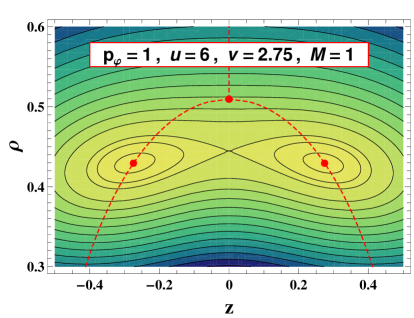
Figure 1: Energy surface defined for $M=1$ (the Coulomb potential) at $p_{z}=p_{\rho}=0$ and $p_{\varphi}=1$. The energy is calculated for $u=\omega_{L}/\omega_{\rho}=6.0$ and for the $3$D system with $v=\omega_{z}/\omega_{\rho}=2.75$. There are two distinct minima at $z\neq 0$. The dashed lines indicate the possible pathes along which the system moves to the symmetric minimum $z_{\mathsf{S}}=0$ with the increase of the angular momentum.

Thus, there are two families of equilibrium states for the relative motion:

• asymmetric states (${\mathsf{A}}$): $(\rho,z)\hskip-1.5pt=\hskip-1.5pt(\rho_{\mathsf{A}},z_{\mathsf{A}})$, $d^{\,2}(u,v)>0$ ;

• symmetric states (${\mathsf{S}}$): $z\hskip-1.5pt=\hskip-1.5ptz_{{\mathsf{S}}}\hskip-1.5pt=\hskip-1.5pt0$.

Note that the condition $d^{\,2}(u,v)>0$ restricts the lower limit of the magnetic field for the existence of the asymmetric states. These states could exist only for the condition

$$d^{\,2}(u,v)>0\Rightarrow\omega_{\rho}{{}^{2}}+\omega_{L}{{}^{2}}\geq\omega_{z}{{}^{2}}.$$ (44)

For the sake of illustration, we calculate the total classical energy for $M=1$ (the Coulomb potential), defined by Eqs.(10,12,13) for fixed values of parameters (see Fig.1). Two asymmetric minima $z\neq 0$ of the Hamiltonian function (10) are exhibited on the energy surface for a given value of the angular momenta ($p_{\varphi}=1$) at the fixed values of the magnetic field ($u$) and the system (QD) size ($v$). For the fixed parameters the increase of the angular momentum value transforms two asymmetric minima $(\rho,z)\hskip-1.5pt=\hskip-1.5pt(\rho_{\mathsf{A}},\pm z_{\mathsf{A}})$ to the symmetric one $(\rho,z)\hskip-1.5pt=\hskip-1.5pt(\rho_{\mathsf{S}},0)$ which moves along the vertical line. We return to this point in next Section.

III.1 Asymmetric states

Let us focus on the family of equilibrium solutions for the asymmetric states. Eq.(42) determines the equilibrium energy of the relative motion

$$\mbox{\rsfs E}_{\,{\mathsf{A}},u,v,M}(p_{\varphi})=\tfrac{1}{2}\,(1+\tfrac{2}{M})\,h_{M,2\,M}(v)+d(u,v)\times|p_{\varphi}|-u\,p_{\varphi}.$$ (45)

Here, the relative energy $\mbox{\rsfs E}_{\,{\mathsf{A}},u,v,M}(x)$ as well as the centre-of-mass energy $\mbox{\rsfs E}_{\,\rm CM}$ (see, Eq.(38)) is defined in $E_{\diamond}$ units. The equilibrium states create the energy hyper-surface in the three-dimensional space of physical external parameters $(u,v,p_{\varphi})$. Evidently, this surface is bounded by the families of $\it symmetric$ states. Our aim is to find a range of the parameters which determine the asymmetric states on the energy hypersurface of extreme states $(\mbox{\rsfs E},u,v,p_{\varphi})$.

To proceed we introduce the following function

$$G_{M}(p_{\varphi},u,v)=h_{M,8}(v)\,{p_{\varphi}}{{}^{2}}-u^{2}+v^{2}.$$ (46)

With the aid of this function let us consider the ratio

$$\rho_{\mathsf{A}}^{4}/r_{\mathsf{A}}{{}^{4}}=(G_{M}(p_{\varphi},u,v)+u^{2}-v^{2})/d^{\,2}(u,v).$$ (47)

Evidently, the condition $G_{M}(p_{\varphi},u,v)=1$ yields the solution $z_{\mathsf{A}}=0$.

Definition 1

. Mapping ${\mathsf{A}}_{u,v}:p_{\varphi}\mapsto{\mathsf{q}}_{u,v,M}(p_{\varphi})$, where ${\mathsf{q}}_{u,v,M}=(r,r{{}_{\ast}})$ and $r:=(\rho,z,p_{\rho},p_{z})$, we call ${\mathsf{A}}_{u,v}$ band. The ranges of the physical parameters $u\,($for convenience, we consider the positive magnetic field $u>0$; see below$)$ and $p_{\varphi}$ are obtained from the inequality:

$$G_{M}(p_{\varphi},u,v)\leq 1.$$ (48)

Points of the set $\Sigma_{\mathsf{A}}(u,v)=\{(u,v,p_{\varphi}),\,G_{M}(p_{\varphi},u,v)=1\}$ we call maximal ${\mathsf{A}}_{u,v}$ states.

The maximal ${\mathsf{A}}_{u,v}$ states are points of the intersection between ${\mathsf{A}}$ and ${\mathsf{S}}$ sets: $\Sigma_{{\mathsf{A}}}\hskip-1.5pt=\hskip-1.5pt{\mathsf{S}}\cap{\mathsf{A}}=\partial{\mathsf{A}}$, i.e., the set $\Sigma_{\mathsf{A}}$ closes the family of ${\mathsf{A}}$ states.

The inequality (48) can be resolved with respect to $u$ or to $p_{\varphi}$:

$$u_{\rm crit}(v,p_{\varphi},M)\leq u\;\;\wedge\;\;|p_{\varphi}|<p_{u,M}(v),$$ (49)

where

$$u_{\rm crit}(v,p_{\varphi},M)=\sqrt{h_{M,8}(v)\,{p_{\varphi}}{{}^{2}}-1+v^{2}},$$ (50)

$$p_{u,M}(v)=d(u,v)\,h_{M,-4}(v).$$ (51)

The transition point from the family of ${\mathsf{S}}$ states to the family ${\mathsf{A}}$ states signals on the spontaneous symmetry breaking with respect to the reflection $(\rho,z)\rightarrow(\rho,-z)$ at a fixed value of $p_{u,M}$. We recall that, in general, the spontaneous symmetry breaking is associated with the symmetry breaking of the system’s ground state, although the symmetries of the Hamiltonian hold true (cf PR ). We are faced with the spontaneous breaking of the inner parity symmetry $\mbox{\rsfs P}_{\rm in}$ at the preserved integral of motion $p_{\varphi}=$const. Thus, there is a coexistence of two families of states which we associate with two phases at a fixed value $p_{\varphi}$, and the set $\Sigma_{\mathsf{A}}(u,v)$ determines the unstable ${\mathsf{S}}$ states. The question arises: what kind of states (${\mathsf{A}}$ or ${\mathsf{S}})$ describes the ground and excited states in the manifold $(u,v,p_{\varphi})$, where the parameters $(u,v)$ are external parameters of the system ? Below we aim to define the family of stable ${\mathsf{S}}$ states and to illuminate the question about the equilibrium states of the system.

III.2 Symmetric states

From the evident relation for the Hamiltonian of the relative motion (see Eqs.(10,12)) we obtain for the symmetric states ${\mathsf{S}}$

$$\partial_{v}{\mbox{\rsfs H}}=z^{2}\bigl{|}_{z_{\mathsf{S}}=0}=0.$$ (52)

It results in that the equilibrium values of the variable $\rho\hskip-1.5pt=\hskip-1.5pt\rho_{\mathsf{S}}$ and the equilibrium energy $\mbox{\rsfs E}\hskip-1.5pt=\hskip-1.5pt\mbox{\rsfs E}_{{\mathsf{S}}}$ have to be independent functions of the external parameter $v$:

$$\partial_{v}\rho_{\mathsf{S}}\hskip-1.5pt=\hskip-1.5pt\partial_{v}\mbox{\rsfs E}_{{\mathsf{S}}}\hskip-1.5pt=\hskip-1.5pt0.$$ (53)

It means that for the maximal states ${\mathsf{A}}_{u,v}$ the Definition 1 serves as a constraint for the definition of values $v=v{{}_{\ast}}$ as a function of the $p_{\varphi},u$ :

$$v=v{{}_{\ast}},\qquad G_{M}(p_{\varphi},u,v{{}_{\ast}})\hskip-1.5pt=\hskip-1.5pt1,$$

such that the transition from the family of ${\mathsf{S}}$ states to the family ${\mathsf{A}}_{u,v}$ can be interpreted as the tendency of the $z$-vibration frequency for ${\mathsf{S}}$ state to approach zero.

All remaining ${\mathsf{S}}$ states are found applying to the elements of sets $\Sigma_{{\mathsf{A}}}(u,v{{}_{\ast}})$ the transformation $T_{\alpha}\!:(u,v{{}_{\ast}},p_{\varphi}=p_{u,M}(v{{}_{\ast}}),\rho_{{\mathsf{S}}},z_{{\mathsf{S}}})\to(u,v=\alpha\,v{{}_{\ast}},p_{\varphi},\rho_{{\mathsf{S}}},z_{\mathsf{S}}),\,1\neq\alpha\in\mathbb{R}_{+}$. We obtain a new set of independent variables $(u,v,v{{}_{\ast}})$ instead of the old one $(u,v,p_{\varphi})$. As a result, the above consideration enables to one to obtain the ${\mathsf{S}}$ family in the following way:

Definition 2

. The space of ${\mathsf{S}}$ states is constructed from $A_{u,v}$ states considering a three–dimensional manifold$:$

$${\mathsf{S}}=\{(p_{\varphi},u,v,v{{}_{\ast}}),\;G_{M}(p_{\varphi},u,v{{}_{\ast}})\hskip-1.5pt=\hskip-1.5pt1,\,v\in\mathbb{R}_{+},\,v{{}_{\ast}}\in\mathbb{R}_{+}\},$$ (54)

We find immediately $(p_{\varphi},u,v,v{{}_{\ast}})\in{\mathsf{A}}_{u,v}\cap{\mathsf{S}}\Leftrightarrow v{{}_{\ast}}\hskip-1.5pt=\hskip-1.5ptv$; hence, the mapping $v{{}_{\ast}}\to p_{\varphi}$,

$$p_{\varphi}=\epsilon_{\varphi}\,p_{u,M}(v{{}_{\ast}}),\quad\epsilon_{\varphi}=\pm 1.$$ (55)

provides the states consistent with Definition 2. Namely, $G_{M}(\epsilon_{\varphi}\,p_{u,M}(v{{}_{\ast}}),u,v{{}_{\ast}})=1$ for $p_{u,M}$ determined by Eq.(51) turns to be the identity relation. Consequently, the expressions for ${\mathsf{S}}$ functions can be found employing the expressions for ${\mathsf{A}}$ functions with the aid of the rule

$$f_{{\mathsf{S}}}(u,v,p_{\varphi},M)\rightarrow f_{{\mathsf{A}}}(u,v{{}_{\ast}},p_{u,M}(v{{}_{\ast}}),M),\qquad f=\rho,\mbox{\rsfs E}.$$ (56)

In particular, Eqs.(42,55) determine an equilibrium value $\rho$: $\rho\hskip-1.5pt=\hskip-1.5pt\rho_{S}(v{{}_{\ast}},M)$; hence,

$$\rho_{S}(v{{}_{\ast}},M)=r_{\mathsf{A}}(p_{u,M}(v{{}_{\ast}}),u,v{{}_{\ast}},M)=h_{M,-2}(v{{}_{\ast}}).$$ (57)

From Eqs.(45,51,56), in the same manner, one obtains the energy of relative motion

$$\mbox{\rsfs E}_{\ast{\mathsf{S}},u,M,\epsilon}(v{{}_{\ast}})=\tfrac{1}{2}\,(1+\tfrac{2}{M})\,h_{M,2\,M}(v{{}_{\ast}})+h_{M,-4}(v{{}_{\ast}})\,d\,(d-\epsilon\,|u|)\,,$$ (58)

where $d\hskip-1.5pt\equiv\hskip-1.5ptd(u,v{{}_{\ast}})$.

The reflection $(p_{\varphi},u)\mapsto(-p_{\varphi},-u)$ is the Hamiltonian symmetry. Therefore, it is convenient to choose a positive magnetic field ($u\geq 0)$, while to analyze both negative and positive values for $p_{\varphi}$. Here $\epsilon\hskip-1.5pt=\hskip-1.5pt\epsilon_{\varphi}\,\epsilon_{u}=\epsilon_{\varphi}$ due to our choice $\epsilon_{u}\hskip-1.5pt=\hskip-1.5pt{\rm sign}\,u=1$.

Evidently, the equilibrium values $(\rho,p_{\varphi},\mbox{\rsfs E}\,)_{\,{\mathsf{S}}}$ do not depend on the variable $v$. The set of equations describing the equilibrium ${\mathsf{S}}$ states with the aid of the variable $v{{}_{\ast}}$ we name the $(u,v,v{{}_{\ast}},\epsilon)$- (or shortly) $v{{}_{\ast}}$-parameterizations of ${\mathsf{S}}$ states.

It is useful to exclude the parameter $v{{}_{\ast}}$. In virtue of definition of $v{{}_{\ast}}$ as the value $v$ of maximal ${\mathsf{A}}_{u,v}$ states (see Definition 1 and Definition 2) and the definition of $G_{M}$ in Eqs.(46), one obtains the following equation for the variable $v{{}_{\ast}}$

$$0=-p_{\varphi}{{}^{2}}+h_{M,4}\,(1+u^{2})\,Z^{4}-h_{M,4}\,Z^{2-M},\qquad Z=h_{M,-2}(v{{}_{\ast}}),$$ (59)

as a function of fixed parameters $(p_{\varphi},u,M)$. In particular, for $M=1$ there is a single real solution

$$v{{}_{\ast}}(p_{\varphi},u,M=1)=Z^{-3/2}(p_{\varphi},u),\quad Z(p_{\varphi},u)=\frac{\sqrt{s}}{2}+\frac{1}{2}\,\sqrt{-s+\frac{2}{\sqrt{s}\,(1+u^{2})}},$$ (60)

$$s=-\frac{4\,2^{1/3}\,p_{\varphi}{{}^{2}}}{Q}+\frac{Q}{3\,2^{1/3}\,(1+u^{2})},$$ (61)

$$Q=\Bigl{(}27+27\,u^{2}+\sqrt{729\,(1+u^{2})^{2}+6912\,p_{\varphi}{{}^{6}}\,(1+u^{2})^{3}}\Bigr{)}^{1/3}.$$ (62)

As a result, for the equilibrium ${\mathsf{S}}$ states one obtains

$$\rho_{\,{\mathsf{S}}}|_{M=1}=v^{-2/3}_{\ast}(p_{\varphi},u,1)\hskip-1.5pt=\hskip-1.5ptZ(p_{\varphi},u).$$ (63)

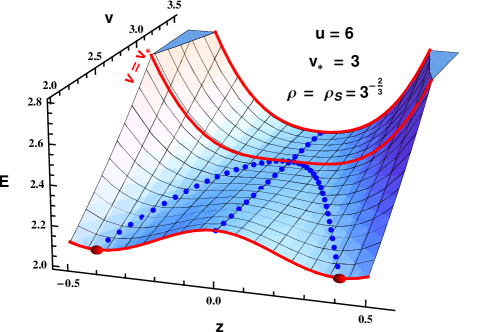
Figure 2: The surface of energy of relative motion studied by means of the $v{{}_{\ast}}$ parametrization for $M\hskip-1.5pt=\hskip-1.5pt1$, $\rho\hskip-1.5pt=\hskip-1.5pt\rho_{{\mathsf{S}}}(3,1)$, and $u=\omega_{L}/\omega_{\rho}=6.$ The energy is given in $E_{\diamond}$ unit.

The parametrization $(u,v,v{{}_{\ast}},\epsilon)$ or $v{{}_{\ast}}$–parametrization is a key element which enables to one to elucidate the shape transition phenomenon. Assuming $M\hskip-1.5pt=\hskip-1.5pt1$, $v{{}_{\ast}}\hskip-1.5pt=\hskip-1.5pt3$ and $\rho\hskip-1.5pt=\hskip-1.5pt\rho_{{\mathsf{S}}}(3,1)$ (see Eq.(57)), with the aid Eqs.(11-13) we consider the energy surface $\mbox{\rsfs E}=\mbox{\rsfs H}_{s,\rm rel}$ at $p_{\rho}=p_{z}=0$ and $(\rho,p_{\varphi})\hskip-1.5pt=\hskip-1.5pt(\rho_{\mathsf{S}}(v{{}_{\ast}},M),p_{u,M}(v{{}_{\ast}}))$ (see Fig.2) as function of $(v,z)$ variables. The magnetic field strength is chosen as $u=\omega_{L}/\omega_{\rho}=6$. Accordingly with Eqs.(52),(58)), along the line $z\hskip-1.5pt=\hskip-1.5pt0$, the energy does not depends on $v$ (dotted line). The curve $v\hskip-1.5pt=\hskip-1.5ptv{{}_{\ast}}\hskip-1.5pt=\hskip-1.5pt3$ divides a plane $(z,v)$ on two domains. For each section $v$ such that $v<v{{}_{\ast}}$ the condition $z\hskip-1.5pt=\hskip-1.5pt0$ corresponds to the saddle point, while the energy minima are asymmetric states: $((v,z_{\mathsf{A}})$, $(v,-z_{\mathsf{A}}))$ (dotted parabolic line). For $v{{}_{\ast}}<v$ the energy has a single minimum at $z\hskip-1.5pt=\hskip-1.5pt0$ only.

A general analysis of the explicit $(u,p_{\varphi})$-representation of ${\mathsf{S}}$ states for the arbitrary $M$ values is given in Appendix A. In virtue of the results obtained in Appendix A, with the aid of Eq.(58) we define the equilibrium energy of ${\mathsf{S}}$ states as a function of the orbital momentum

$$\mbox{\rsfs E}_{\,{\mathsf{S}},u,v,M}(p_{\varphi})=\mbox{\rsfs E}_{\ast S,u,M,{\rm sign}(p_{\varphi})}\circ v{{}_{\ast}}(p_{\varphi},u,M).$$ (64)

By the analogy with the expression (45) for the energy of ${\mathsf{A}}$ states we include the index $v$ which is a dummy parameter due to the condition Eq.(52).

III.3 Minimal states in the classical limit

In the classical limit, at fixed physical parameters ($\omega_{\rho}$, $\omega_{z})$ of the confined system, (i.e., $v=\omega_{z}/\omega_{\rho}$ is fixed), we search minimal energy states at a given value of the magnetic field ($\omega_{L}\Rightarrow u=\omega_{L}/\omega_{\rho}$) with respect to the integrals of motion $p_{\varphi},p_{\varphi\ast}$.

The energy of center-of-mass motion (38) is minimal at $p_{\varphi\ast}=0$. Evidently, it does not contribute to the total energy in the classical limit. Let $p_{\varphi,\rm min}$ be a value of the orbital momentum $p_{\varphi}$ minimizing the relative motion energy. Eqs.(33,34) yield

$$0\hskip-1.5pt=\hskip-1.5pt\rho^{2}\,\dot{\varphi}=p_{\varphi,\rm min}-\rho_{{\mathsf{X}}}{{}^{2}}\,u,\qquad{\mathsf{X}}={\mathsf{S,A}}.$$ (65)

Note that for the ${\mathsf{S}}$ states Eq.(65) holds only for $p_{\varphi,\rm min}>0$ (see Eq.(55)). In virtue of this fact, with the aid of Eqs.(65),(51),(57), one obtains that $v{{}_{\ast}}=1$. Taking into account the definition of energies Eqs.(45),(58), we have finally

$$(p_{\varphi},\rho^{2},\mbox{\rsfs E}_{\,\rm rel},{\mathsf{X}})_{\rm min}=\begin{cases}(0,0,\tfrac{1}{2}\,(1+\tfrac{2}{M})\,h_{M,2\,M}(v),\,{\mathsf{A}})|_{M\hskip-1.5pt=\hskip-1.5pt1}=(0,0,\tfrac{3}{2}\,v^{2/3},{\mathsf{A}})&v\leq 1\\ (u,1,\,\tfrac{1}{2}\,(1+\tfrac{2}{M}),\,{\mathsf{S}})|_{M\hskip-1.5pt=\hskip-1.5pt1}=(u,1,\tfrac{3}{2},{\mathsf{S}})&v>1,\end{cases}$$ (66)

Thus, in the classical limit the ground states of the confined system (in particular, two-electron QD) exhibit diamagnetic properties in the both phases: $\partial_{B}\,E_{\rm tot}\sim\partial_{u}\mbox{\rsfs E}_{\;\rm tot}=0$.

For arbitrary values $u,v$, a collection formula (66) determines a single prescribed value of $p_{\varphi}$ for the minimal state. For $v<1$ the ground state is the ${\mathsf{A}}$ minimal state. For $v\hskip-1.5pt=\hskip-1.5pt1$ the ground state belongs to the ${\mathsf{A}}\cap{\mathsf{S}}$. For $1<v$ the ground state is the ${\mathsf{S}}$ state.

The family of minimal ${\mathsf{S}}$ states provides a simple relation between the strength of the magnetic field and the value of the total angular momentum $L_{z}$:

$$B\sim L_{z}\Rightarrow B=\mbox{\rsfs B}_{\diamond}\,L_{z}.$$

Let us define the constant $\mbox{\rsfs B}_{\diamond}$. Taking into account that $L_{z}\hskip-1.5pt=\hskip-1.5ptp_{\varphi}\,L_{\diamond}$, $B=u\,B_{\diamond}$, $q_{\diamond}\hskip-1.5pt=\hskip-1.5pt\hbar/L_{\diamond}$ (see, Eqs.(8,9)), and $p_{\varphi}\hskip-1.5pt=\hskip-1.5ptu$ (see, Eq.(66)) we have

$$\mbox{\rsfs B}_{\diamond}=B_{\diamond}/L_{\diamond}\quad\Longrightarrow\quad B_{\bullet}=q_{\diamond}\,B_{\diamond}.$$ (67)

As a result, we obtain a magnitude of the magnetic field $B_{\bullet}\hskip-1.5pt=\hskip-1.5pt\hbar\,\mbox{\rsfs B}_{\diamond}\hskip-1.5pt=\hskip-1.5pt\Delta B_{L_{z}\to L_{z}+\hbar}$ which yields a change of the angular momentum on one Planck unit. For $M=1$ (the Coulomb interaction) it gives

$$B_{\bullet}\approx 0.724\times\bigl{(}\tfrac{m{{}^{\ast}}}{m_{\rm e}}\,\varepsilon_{r}\bigr{)}^{2/3}\,\bigl{(}\tfrac{\hbar\,\omega_{\rho}}{\rm meV}\bigr{)}^{4/3}\times{\rm Tesla}.$$ (68)

IV Vibrational corrections in the harmonic limit

IV.1 Normal modes in the classical limit

As it discussed above, in physical systems, a particle undergoes small oscillations around an equilibrium point. Let us introduce the deviation from equilibrium point ${\mathsf{q}}_{\mathsf{X}}$ $({\mathsf{X}}={\mathsf{A}},{\mathsf{S}})$: ${\mathsf{q}}\hskip-1.5pt=\hskip-1.5pt{\mathsf{q}}_{\mathsf{X}}+{\mathsf{\tilde{q}}}$. As a result, the Hamiltonian function takes the form of the Taylor series

$$\mbox{\rsfs H}\,({\mathsf{q}}_{X}+{\mathsf{\tilde{q}}})=\mbox{\rsfs H}\,({\mathsf{q}}_{X})+\mbox{$\sum\limits_{\alpha}$}(\partial_{\alpha}\mbox{\rsfs H}\,)({\mathsf{q}}_{\mathsf{X}})\,\tilde{q}_{\alpha}+\tfrac{1}{2}\,\mbox{$\sum\limits_{\alpha}$}\mbox{$\sum\limits_{\beta}$}(\partial_{\alpha}\partial_{\beta}\mbox{\rsfs H}\,)({\mathsf{q}}_{\mathsf{X}})\,\tilde{q}_{\alpha}\,\tilde{q}_{\beta}+\ldots,$$

where the stability of the equilibrium solutions requires that the Hessian matrix $(\partial_{\alpha}\partial_{\beta}\mbox{\rsfs H}\;)({\mathsf{q_{0}}})$ should be positively defined. Due to the axial symmetry of our system ($\dot{p}_{\varphi}\hskip-1.5pt=\hskip-1.5pt0$) the deviations are considered for elements of the subset ${\mathsf{q}}$ which form the $\rm SO(2)$ reduced phase space ${\mathsf{q}}\hskip-1.5pt=\hskip-1.5pt\{\rho,z,p_{\rho},p_{z},\rho{{}_{\ast}},z{{}_{\ast}},p_{\rho\ast},p_{z\ast}\}$ (see Sec.II). Taking into account the equilibrium solutions $\mbox{\rsfs E}_{\,{\mathsf{X}}}$ (see Eqs.(38,45,58)) we obtain

$$\mbox{\rsfs H}_{\mathsf{\;X}}=\mbox{\rsfs E}_{\,{\mathsf{X}}}+\mbox{\rsfs E}_{\,{\mathsf{CM}}}+\tfrac{1}{2}\,\mbox{$\sum\limits_{\alpha}$}\,(\tilde{p}_{\alpha}{{}^{2}}+\tilde{p}_{\alpha\ast}{{}^{2}})+\mbox{$\sum\limits_{n=2}$}\mbox{\rsfs U}^{\,(n)}_{{\mathsf{X}}}(\tilde{\rho},\tilde{z})+\mbox{\rsfs U}_{\rm CM}(\tilde{\rho}{{}_{\ast}},\tilde{z}{{}_{\ast}})+u\,\mbox{\rsfs E}_{S}\,M_{S}+\dots,$$ (69)

where the index $(n)$ denotes the approximation order for the potential function $\mbox{\rsfs U}_{\mathsf{X}}$.

In order to analyse the stability of the classical equilibrium, we consider the vibrational modes in the harmonic limit $n\hskip-1.5pt=\hskip-1.5pt2$ and introduce the following definitions

$$\mbox{\rsfs U}^{\,(2)}_{\mathsf{X}}(\tilde{\rho},\tilde{z})=\mbox{\rsfs U}_{\mathsf{X}}=\tfrac{1}{2}\,\mbox{$\sum\limits_{\alpha,\beta}$}\,{\rm k}_{{\mathsf{X}},\alpha\beta}\,\tilde{x}_{\alpha}\,\tilde{x}_{\beta},\qquad\mbox{\rsfs U}_{\mathsf{CM}}(\tilde{\rho},\tilde{z})=\tfrac{1}{2}\,\mbox{$\sum\limits_{\alpha,\beta}$}\,{\rm k}_{{\rm CM},\alpha\beta}\,\tilde{x}_{\alpha\ast}\,\tilde{x}_{\beta\ast},$$ (70)

For the center-of mass-motion we find

$${\mathsf{k}}_{\rm CM}={\rm diag}\,(\Omega_{\rho\ast}{{}^{2}},\Omega_{z\ast}{{}^{2}}),\quad\binom{\Omega_{\rho\ast}}{\Omega_{z\ast}}=\binom{2\,\sqrt{1+u^{2}}}{v}.$$ (71)

For the family of ${\mathsf{A}}$ states we have the following matrix elements

$${\rm k}_{{\mathsf{A}},\rho\rho}=A+4\,d^{\,2}(u,v),\qquad{\rm k}_{{\mathsf{A}},zz}=(M+2)\,v^{2}-A,$$ (72)

$${\rm k}_{{\mathsf{A}},\rho z}={\rm k}_{{\mathsf{A}},z\rho}=(M+2)\,h_{M,2\,(M+4)}(v)\,\rho_{A}\,z_{A},$$ (73)

where $A\hskip-1.5pt=\hskip-1.5pt(2+M)\,\rho_{\mathsf{A}}{{}^{2}}\,h_{M,2\,(4+M)}(v)$, and $\rho_{\mathsf{A}},z_{\mathsf{A}}$ are given by Eq.(42).

We recall that the conditions: Eq.(44) and $p_{\varphi}\leq p_{u,M}(v)$ (see Eq.(51)), – determine the admissible domain of ${\mathsf{A}}$ states. At these conditions the matrix ${\mathsf{k}}_{\mathsf{A}}$ is well defined and yields the following eigenmodes $\Omega_{\pm,{\mathsf{A}}}$:

$$\Omega_{\pm,{\mathsf{A}},u,v,M}{{}^{2}}(p_{\varphi})=\tfrac{1}{2}\,[4(1+u^{2})+(M-2)\,v^{2}\pm\sqrt{[4(1+u^{2})-(6+M)\,v^{2}]^{2}+\Delta^{2}}\,],$$ (74)

$$\Delta^{2}=16\,(2+M)\,h_{M,2(4+M)}(v)\,d(u,v)\,|p_{\varphi}|.$$ (75)

Thus, in terms of normal modes, for the ${\mathsf{A}}$ states we obtain

$$\mbox{\rsfs U}_{\mathsf{A}}^{\;\prime}=\tfrac{1}{2}\,(\Omega_{-,A}{{}^{2}}\,\tilde{x}_{-}{{}^{2}}+\Omega_{+,A}{{}^{2}}\,\tilde{x}_{+}{{}^{2}}),\qquad\binom{\tilde{z}_{+}}{\tilde{z}_{-}}=\biggl{(}\begin{matrix}{\hphantom{-}}\cos\phi&\sin\phi\\ -\sin\phi&\cos\phi\end{matrix}\biggr{)}\cdot\binom{\tilde{z}_{\rho}}{\tilde{z}_{z}},$$ (76)

where $\phi=\tfrac{1}{2}\,{\rm arctan}\,[2{\rm k}_{{\mathsf{A}},\rho z}/({\rm k}_{{\mathsf{A}},\rho\rho}-{\rm k}_{{\mathsf{A}},zz})]$ and $\tilde{z}\hskip-1.5pt=\hskip-1.5pt\tilde{x},\,\tilde{p}$.

Note that the equilibrium ${\mathsf{S}}$ states are defined by the equilibrium parameter $v{{}_{\ast}}$ by means of the $v{{}_{\ast}}$-parameterizations (see Eq.(58) and the following discussion in Sec.IIIB). The expansion (70) for the ${\mathsf{S}}$ states in $(\rho,z)$-representation has a diagonal form

$${\mathsf{k}}_{\mathsf{S}}={\rm diag}\,(\Omega_{\rho,{\mathsf{S}}}{{}^{2}},\,\Omega_{z,{\mathsf{S}}}{{}^{2}}),$$ (77)

$$\Omega_{\alpha,{\mathsf{S}}}\hskip-1.5pt\equiv\hskip-1.5pt\Omega_{\alpha,{\mathsf{S}},u,v,M}(p_{\varphi})=\Omega_{\alpha,\ast{\mathsf{S}},u,v,M}\circ v{{}_{\ast}}(p_{\varphi},u,M),\quad\alpha=\rho,z,$$ (78)

where

$$\Omega_{z,\ast{\mathsf{S}}}=\sqrt{v^{2}-v{{}_{\ast}}{{}^{2}}},\qquad\Omega_{\rho,\ast{\mathsf{S}}}=\sqrt{4\,(1+u^{2})+(M-2)\,v{{}_{\ast}}^{2}}.$$ (79)

Here, $\Omega_{\alpha,\ast{\mathsf{S}}}\hskip-1.5pt\equiv\hskip-1.5pt\Omega_{\alpha,\ast{\mathsf{S}},u,v,M}(v{{}_{\ast}})$. Evidently, the expansion (70) of the ${\mathsf{S}}$ states (which approaching the maximal ${\mathsf{A}}_{u,v}$ states) takes place around the equilibrium parameters of the confined system ($v=\omega_{z}/\omega_{\rho})$ such as $v=v{{}_{\ast}}$. In this case one of the normal modes $\Omega_{z,\ast{\mathsf{S}}}\equiv 0$ (see Eq.(79)) and it follows that

• for $v{{}_{\ast}}<v$ we have stable ${\mathsf{S}}$ states, which we denote as ${\mathsf{S}}_{+}$;

• the condition $v\hskip-1.5pt=\hskip-1.5ptv{{}_{\ast}}$ defines the bifurcation point at a given value of the magnetic field $\omega_{L}$, which determines the subfamily of ${\mathsf{S}}$ denoted as ${\mathsf{S}}_{0}$;

• the condition $v<v{{}_{\ast}}$ defines the unstable ${\mathsf{S}}$ states (saddle points) denoted as ${\mathsf{S}}_{-}$.

We name the points (a,b,c) as Rules I. In general, the condition $v\hskip-1.5pt=\hskip-1.5ptv{{}_{\ast}}$ defines a shape (phase) transition surface in the three-dimensional space $(u,v,p_{\varphi})$ (see also Fig.2). Thus, the plane $v\hskip-1.5pt=\hskip-1.5ptv{{}_{\ast}}$ divides the ${\mathsf{S}}$ manifold on three sets ${\mathsf{S}}\hskip-1.5pt=\hskip-1.5pt{\mathsf{S}}_{-}\cup{\mathsf{S}}_{0}\cup{\mathsf{S}}_{+}$ accordingly to the value of parameter $\mu\hskip-1.5pt=\hskip-1.5pt{\rm sign}\,(v-v{{}_{\ast}})$. The application of Rules I will be discussed in details for a particular case in Sec.V.A (see below Fig.3).

Since the maximal ${\mathsf{A}}_{u,v}$ states define the phase transition hypersurface $G_{M}(p_{\varphi},u,v)\hskip-1.5pt=\hskip-1.5pt1$ in three–dimensional space $(u,v,p_{\varphi})$, in a number of applications it is instructive to use $u_{\rm crit}(v,p_{\varphi},M)$, Eq.(50). Note that for $p_{\varphi}=0$ Eq.(50) yields $u_{0}=u_{\rm crit}(v,p_{\varphi}=0,M)=\sqrt{v^{2}-1}$ which is fulfilled for a standard choice of the QD parameters : $\omega_{\rho}\ll\omega_{z}$. Thus, we conclude that for $u_{0}<u$ and at the condition (51) one expects the asymmetric ${\mathsf{A}}$ states. Taking into account quantum oscillations around the equilibrium classical ground states, we may expect a shape (phase) transition from ${\mathsf{S}}$- to ${\mathsf{A}}$- states at the magnetic field strength $u>u_{0}$ for orbital momenta $p_{\varphi}<p_{u,M}$ (see Eq.(51)). Thus, if the system’s parameters are subject to the condition $q_{\diamond}<1$ , when the harmonic approximation is well justified, we predict a shape transtion from a lateral to a vertical localization of two confined fermions in a magnetic field. This general conclusion elucidates the shape transition in the excited state found for two-electron QDs in the magnetic field ent . Indeed, this excited state is formed in the local potential minimum produced by the interplay of the parabolic three-dimensional confinement, the magnetic field and the Coulomb interaction.

IV.2 Quantization of normal modes

To quantize normal modes of the classical Hamiltonian in the form $h_{\alpha}(\Omega_{\alpha})=\tfrac{1}{2}\,(p_{\alpha}{{}^{2}}+\Omega_{\alpha}{{}^{2}}\,x_{\alpha}{{}^{2}})$ we follow the standard procedure. The latter is established by means of following expressions

$$\binom{\hat{x}_{a}}{\hat{p}_{a}}=\sqrt{\frac{q_{\diamond}}{2}}\,\binom{{\hphantom{-}}\bar{\omega}_{a}{{}^{-1/2}}\,\hat{B}_{a+}}{-i\,\bar{\omega}_{a}{{}^{1/2}}\,\hat{B}_{a-}},\quad a=\pm,\rho,z$$ (80)

$$\hskip 5.69054pt\hat{B}_{a\pm}=\pm e^{i\,\psi_{a}/2}\,\hat{b}_{a}{{}^{\dagger}}(\bar{\omega}_{a})+e^{-i\,\psi_{a}/2}\,\hat{b}_{a}(\bar{\omega}_{b}).$$

The phases $\psi_{\alpha}$ provide the phase convention for states $\langle\tilde{x}_{\alpha}|n\rangle$. We fix the phases by the conditions $\psi_{\alpha}\hskip-1.5pt=\hskip-1.5pt\psi_{\alpha{{}_{\ast}}}\hskip-1.5pt=\hskip-1.5pt0$.

In virtue of the Poisson rules (see, Eq.(22) and the text below Eq.(17)) and the representation (80) one obtains

$$[\hat{B}_{a-},\hat{B}_{a+}]\hskip-1.5pt=\hskip-1.5pt2\,[\hat{b}_{a},\hat{b}_{b}{{}^{\dagger}}]=2\,\delta_{ab}\,.$$

Thus, the operators $\hat{b}_{\alpha},\hat{b}^{\dagger}_{\beta}$ obey the standard boson commutation relations with respect to the boson vacuum $\hat{b}_{\alpha}|0\rangle=0$. As a result we have

$$\hat{h}(\bar{\omega},\Omega)=\tfrac{q_{\diamond}}{4}\,(\Omega^{2}/\bar{\omega}+\bar{\omega})(\hat{b}^{\dagger}\,\hat{b}+\hat{b}\,\hat{b}^{\dagger})+\tfrac{q_{\diamond}}{4}\,(\Omega^{2}/\bar{\omega}-\bar{\omega})((\hat{b}^{\dagger})^{2}+\hat{b}{{}^{2}}),$$

where $\bar{\omega}$ is a positive parameter. The minimization of the energy $\mbox{\rsfs E}_{\bar{\omega}_{\rho},\bar{\omega}_{z}}(k_{\rho},k_{z})\hskip-1.5pt=\hskip-1.5pt\langle\Sigma_{\alpha}\hat{h}_{\alpha}(\bar{\omega}_{\alpha},\Omega_{\alpha})\rangle\hskip-1.5pt=\hskip-1.5pt\tfrac{q_{\diamond}}{4}\,\Sigma_{\alpha}(\Omega_{a}{{}^{2}}/\bar{\omega}_{\alpha}+\bar{\omega}_{a})\,(2\,k_{\alpha}+1)$ with respect to $\bar{\omega}_{\rho},\bar{\omega}_{z}$ yields the result $\bar{\omega}_{\alpha}\hskip-1.5pt=\hskip-1.5pt\sqrt{\Omega_{a}{{}^{2}}}$. Thus, the minimum exists only for $\Omega_{a}{{}^{2}}>0$.

It is noteworthy that the relation $L_{z}\hskip-1.5pt=\hskip-1.5ptp_{\varphi}\,L_{\diamond}$ (see also Eq.(9)) provides a natural quantization of the orbital momentum:

$$L_{z}\hskip-1.5pt=\hskip-1.5pt\frac{p_{\varphi}}{q_{\diamond}}\hbar\Rightarrow p_{\varphi}/q_{\diamond}=m=0,\pm 1,\ldots,\qquad p_{\varphi\ast}/q_{\diamond}=m{{}_{\ast}}=0,\pm 1,\ldots.$$ (81)

In general, the total energy has the following form

$$\mbox{\rsfs E}^{\,(n)}_{\;{\mathsf{tot}},{\mathsf{k}},{\mathsf{k}}{{}_{\ast}},M_{S}}({\mathsf{w}})=\mbox{\rsfs E}_{\,{\rm CM},u,{\mathsf{k}}{{}_{\ast}}}+\mbox{\rsfs E}^{\;(n)}_{\;{\mathsf{X}},u,v,q_{\diamond},M,{\mathsf{k}}}+u\,\mbox{\rsfs E}_{S}\,M_{S},$$ (82)

$${\mathsf{X}}\equiv{\mathsf{X}}(u,v,m,q_{\diamond},M)=\begin{cases}{\mathsf{A}}&\text{if~{}}G_{M}(m\,q_{\diamond},u,v)<1,\\ {\mathsf{S}}&\text{else},\end{cases}$$ (83)

where ${\mathsf{w}}\equiv(u,v,q_{\diamond},M)$, and the number $(n)$ defines the order of approximation. Here, ${\mathsf{k}}\hskip-1.5pt=\hskip-1.5pt(k_{\rho},k_{z},m)$, ${\mathsf{k}}{{}_{\ast}}\hskip-1.5pt=\hskip-1.5pt(k_{\rho\ast},k_{z\ast},m{{}_{\ast}})$, where $(k_{\rho},k_{z},k_{\rho\ast},k_{z\ast}$) are harmonic oscillator quantum numbers ($k_{a},k_{a\ast}=0,1,\ldots$), and $M_{S}\hskip-1.5pt=\hskip-1.5pt0,\pm 1$ is a z-projection of the total spin of pair electrons.

The eigenenergies of the center-of-mass motion are defined as

$$\mbox{\rsfs E}_{\,{\rm CM},u,{\mathsf{k}}{{}_{\ast}}}=\bigl{[}\sqrt{1+u^{2}}\,(|m{{}_{\ast}}|+2\,k_{\rho\ast}+1)-u\,m{{}_{\ast}}+(\tfrac{1}{2}+k_{z\ast})\,v\bigr{]}\times q_{\diamond}.$$ (84)

For $q_{\diamond}=1$ these energies are well-known Fock-Darwin ones (see, for example, naz ). Taking into account Eq.(81), we have for the energy of relative motion in the harmonic limit ($n\hskip-1.5pt=\hskip-1.5pt2$)

$$\mbox{\rsfs E}^{\;(2)}_{\,{\mathsf{X}},u,v,q_{\diamond},M,{\mathsf{k}}}=\mbox{\rsfs E}_{\,{\mathsf{X}},u,v,M}(m\,q_{\diamond})+q_{\diamond}\times\mbox{$\sum\limits_{\alpha}$}\;\Omega_{\alpha,{\mathsf{X}},u,v,M}(m\,q_{\diamond})\,(k_{\alpha}+\tfrac{1}{2}).$$ (85)

We recall, that the classical energy $\mbox{\rsfs E}_{\,{\mathsf{X}},u,v,M}(p_{\varphi})$ for ${\mathsf{X}}={\mathsf{A}}$, ${\mathsf{S}}$ are defined by Eqs.(45,64), respectively. The normal modes $\Omega_{\alpha,{\mathsf{X}}}$ for ${\mathsf{X}}={\mathsf{A}},{\mathsf{S}}$ are defined by Eqs.(74,78), respectively.

V Analysis of results

For the sake of illustration of general results obtained for the potential $\mbox{\rsfs U}_{M}({\mathsf{r}})=\alpha_{M}\,{\mathsf{r}}^{-M}$$(\alpha_{M}>0)$ we consider the most studied case of $M=1$ (the Coulomb potential). We compare our analytical results with the numerical results obtained previously for the three-dimensional two-electron QDs nen3 for different $q_{\diamond}$ values. This analysis will allow also to illuminate the details of the interplay between the classical and quantum mechanical dynamics in realistic samples.

V.1 Classical limit

First, let us discuss the equilibrium classical energy $\mbox{\rsfs E}_{{\mathsf{S}},u,v,M\hskip-1.5pt=\hskip-1.5pt1}(p_{\varphi})$ (see Eq.(64)) for the ${\mathsf{S}}$ states. Fig.3 displays the energy surface for the two-electron QD at different values of the magnetic field $u$ and for various values of the orbital momentum $p_{\varphi}$.

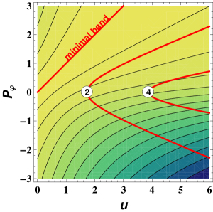
Figure 3: $(u,p_{\varphi})$ projection of contours of energy $\mbox{\rsfs E}_{\,{\mathsf{S}}}$. The energy grows from the minimal band, and each line, starting from the minimal band, corresponds to the increase of the energy on one unit of $E_{\diamond}$.

The straight line displays the minimal energy of the ${\mathsf{S}}$-states in the classical limit. According to Eqs.(65,66) this line is obtained from the requirement $(\partial_{p_{\varphi}}\,\mbox{\rsfs E}\;)_{\,{\mathsf{S}},u,v,M}(p_{\varphi})=0$ at the condition $v{{}_{\ast}}=1$. The minimal states have definite values of the orbital momentum, which are subject to the condition $p_{\varphi}=u$ for $M=1$.

Once we fix the size of the QD $v=\omega_{z}/\omega_{\rho}$, the Rules I (see Sec.IV.1) take place. These rules are manifested through the hyperbolic (thick) lines $v{{}_{\ast}}\hskip-1.5pt=\hskip-1.5pt{\rm const}$ which divide the regions of stable and unstable ${\mathsf{S}}$ states for various values of the orbital momentum $p_{\varphi}$ that are available at various values of the magnetic field $u$. The lines are obtained by means of the solution of the equation for different values of $u$

$$u^{2}-h_{M,4}(v{{}_{\ast}})\,{p_{\varphi}}{{}^{2}}=v^{2}-1,$$

where $h_{M,r}(v)$ is given by Eq.(4). This equation represents the condition: $1\hskip-1.5pt=\hskip-1.5ptG_{M}(p_{\varphi},u,v)$ (see Eq.(46) and Eq.(54)) for $h_{M,r}(v)$.

The lines are labelled by corresponding $v{{}_{\ast}}$ numbers. For example, for the QD size $v_{1}$, defined by the condition $v{{}_{\ast}}=1\leq v_{1}\leq v{{}_{\ast}}=2$, the minimal ${\mathsf{S}}$-states are stable for all values of the magnetic field $u$ and the orbital momenta $p_{\varphi}$ on the surface region $(u,p_{\varphi})$ restricted by the lines: ”minimal band” and $2$. All ${\mathsf{S}}$-states, which energies are higher those of the minimal band, are vibrational excitations relative to the states of the minimal band. Evidently, for $v_{1}$ the right region on the surface $(u,p_{\varphi})$ restricted by the line 2 is associated with the stable ${\mathsf{A}}$-states, according to the Rules I c.

For the QD size $v_{2}$, defined by the condition $v_{2}\leq v{{}_{\ast}}=4$, the admissible domain of values on the $(u,p_{\varphi})$-surface is defined by the lower limit which is the line ”minimal band” and the upper limit which is the line $4$. Again, the Rules I are applied to distinguish stable ${\mathsf{S}}$– and ${\mathsf{A}}$–states for the QD size $v_{2}$.

V.2 Validity of the model: a comparison with numerical calculations

The ground state energy of a QD, as a function of magnetic field, is studied by means of single-electron capacitance spectroscopy or by single-electron tunneling spectroscopy (see for review kou ). At low temperature $\sim 100$ mK, a large electrostatic charging energy prevents the flow of current and, therefore, the dot has a fixed number of electrons. Applying a gate voltage to the contacts brings the electro-chemical potential of the contacts in resonance with the energy $\mu(N)$ that is necessary for adding the $N$-th electron, tunneling through the barrier, into the dot with $N-1$ electrons. As a result, one observes experimentally kinks in the additional energy

$$E_{\rm add}(N)=\mu(N)-\mu(N-1),$$

where $\mu(N)=E(N)-E(N-1)$ is an electrochemical potential and $E(N)$ is the total ground state energy of an $N$-electron dot. For $N\hskip-1.5pt=\hskip-1.5pt2$ we have: $E(0)\hskip-1.5pt=\hskip-1.5pt0$, $E(1)\hskip-1.5pt=\hskip-1.5ptE_{\rm CM}$, $E_{\rm add}(2)\hskip-1.5pt=\hskip-1.5ptE_{\rm rel}-E_{\rm CM}$. Hence, according to Eq.(83), we have

$$\mbox{\rsfs E}^{\;(n=2)}_{\,{\mathsf{add}},{\mathsf{k}},{\mathsf{k}}{{}_{\ast}},M_{S}}({\mathsf{w}})=-\mbox{\rsfs E}_{\,{\rm CM},u,{\mathsf{k}}{{}_{\ast}}}+\mbox{\rsfs E}^{\;(n=2)}_{\;{\mathsf{X}},u,v,q_{\diamond},M,{\mathsf{k}}}+u\,\mbox{\rsfs E}_{S}\,M_{S},$$ (86)

where ${\mathsf{X}}\hskip-1.5pt\equiv\hskip-1.5pt{\mathsf{X}}(u,v,m,q_{\diamond},M)$ is defined in Eq.(83). In order to define the quantum number $M_{S}$ we have to take into account the Pauli principle. The spatial symmetry of wave function $\Psi({\mathsf{x}}_{1},{\mathsf{x}}_{2})$ under the permutation of electrons is determined by the phase factor $(-1)^{m+k_{z}}$ . We consider a standard situation, when the confinement in z direction is much stronger than the lateral one, i.e., $\omega_{z}\gg\omega_{\rho}$. Therefore, the lowest quantum numbers for the $z$-confinement are important only for the ground state transitions of the QD in the magnetic field nen3 ; nen4 . For $k_{z}\hskip-1.5pt=\hskip-1.5pt0$ the total wave function is antisymmetric, if $(-1)^{S+m}\hskip-1.5pt=\hskip-1.5pt1$. Since $M_{S}=-S$, the rule

$$M_{S}\hskip-1.5pt=\hskip-1.5pt-{\rm mod}_{2}(m),$$

determines quantum number $M_{S}$ of the minimal antisymmetric states.

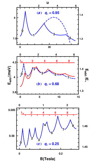
Figure 4: The additional energy as a function of the $q_{\diamond}$-factor for different values of the magnetic field $B(u)$. The following confinement parameters $\hbar(\omega_{\rho},\omega_{z})$ are chosen: (a) 5.5,22; (b) 2,8; (c) 0.1, 4 (meV). All calculations are done for $m{{}_{\ast}}=0.067\,m_{e},\epsilon\hskip-1.5pt=\hskip-1.5pt12,|g|\hskip-1.5pt=\hskip-1.5pt0.3$. Panel (a): the evolution of $m=1$ state as function of the magnetic field, after a crossing of the state $m=3$, is displayed by dashed line. Panel (b): solid and dashed lines are used for the analytical and numerical results for two-electron QD nen3 , respectively. The straight lines in panels (b), (c) display the values of the orbital momentum of the minimal state as a function of the magnetic field.

As it is discussed in Sec.I, the quantity $q_{\diamond}$ defined in Eq.(8), characterizes the strength of the quantum effects over the classical ones. The results of calculations of the additional energies are shown on Fig.4 for various values of the $q_{\diamond}$-factor (the Coulomb interaction). The calculations are done at different values of the magnetic field $B$ (in ${\rm Tesla}$, bottom) which are related to the dimensionless parameter $u$ (top). The left scale counts energy in ${\rm meV}$, while the right one expresses the energy in the $E_{\diamond}$ unit. The straight lines in Figs.4(b),(c), demonstrate the angular momentum scale obtained with aid of Eqs.(III.3,68), and represent a classical limit.

For the Coulomb interaction, at almost equal strengths of the classical and quantum effects (see Fig.4(a)), the harmonic approximation fails with the increase of the magnetic field. The state with $m\hskip-1.5pt=\hskip-1.5pt1$ becomes lower than the state $m\hskip-1.5pt=\hskip-1.5pt5$ at high values of the magnetic field $B>35$ Tesla. This behaviour of the energy, defined at fixed value $v$ and $p_{\varphi}=p_{m}\hskip-1.5pt=\hskip-1.5ptm\,q_{\diamond}$, indicates that the parameter $u$ is close to the critical value $\bar{u}\hskip-1.5pt=\hskip-1.5ptu_{\rm crit}(v,p_{m},M)$ (see Eq.(50)).

To illuminate this fact we analyse the limit $u\to\Omega_{z}$ for fixed values $v,p_{\varphi}$. For ${\mathsf{S}}$ states, at the neighborhood of the critical values the definition (54) reads : $1\hskip-1.5pt=\hskip-1.5ptG_{M}(p_{m},\bar{u}+z,v{{}_{\ast}}),\,v{{}_{\ast}}=v+V(z)$, where $V(0)\hskip-1.5pt=\hskip-1.5pt0$ and $0<\Omega_{z,{\mathsf{S}}}\Leftrightarrow z<0$. The derivative of function $V(z)$ is obtained by means of the theorem on implicit function: $0=G_{M}{}^{(0,1,0)}dz+G_{M}{}^{(0,0,1)}dV\Rightarrow V^{\prime}(0)=-G_{M}{}^{(0,1,0)}(p_{m},\bar{u},v)/G_{M}{}^{(0,0,1)}(p_{m},\bar{u},v)$. Since the exact analytical form of $\Omega_{z,S}$ is unknown in general, we obtain the result with the aid of the $v{{}_{\ast}}$ parametrization $\Omega_{z,\ast{\mathsf{S}}}$ (see Eq.(79)),

$$\Omega_{z,S}{{}^{2}}\hskip-1.5pt=\hskip-1.5pt\Omega_{z,\ast{\mathsf{S}}}{{}^{2}}\hskip-1.5pt\approx\hskip-1.5pt-2\,v\,V^{\prime}(0)\,\delta u,\qquad\;V^{\prime}(0)=\frac{\bar{u}\,v}{v^{2}+z_{M}(p_{\varphi},v)}\,,$$

where $z\hskip-1.5pt\equiv\hskip-1.5ptz_{M}(p,v)\hskip-1.5pt=\hskip-1.5pt4\,p{{}^{\,2}}\,h_{M,8}(v)/(2+M)$. If $0<\delta u$ then we deal with the phase ${\mathsf{A}}$. The expansion of $\Omega_{z,{\mathsf{A}},\bar{u}+\delta u,v,M}(p_{m})$ for $0<\delta u$ is determined directly from Eq.(74). Comparing both result we obtain

$$\Omega_{z,\bar{u}+\delta u,v,M}(p_{m})\hskip-1.5pt\approx\hskip-1.5pt\sqrt{v\,V^{\prime}(0)}\times\begin{cases}\sqrt{-2\,\delta u}&\delta u\leq 0,\\ \hfill 2\,\sqrt{\delta u}\hfill&\text{else}.\end{cases}$$

Note that the function $\delta u\to-\Omega_{z,\bar{u}+\delta u,v}(p_{m})$ defines curves which are similar to a “$\lambda$” letter. As a result, the derivative $(\partial_{u}\Omega_{z})_{u,v,M}(p_{m})$ does not exist at $u\hskip-1.5pt=\hskip-1.5ptu_{\rm crit}(v,p_{m},M)$.

It proves that the harmonic approach is broken down in the domain $|\delta u|\ll 1$. More precisely, the assumption that $\mbox{\rsfs E}^{\,(2)}_{{\mathsf{tot}},{\mathsf{k}},{\mathsf{k}}{{}_{\ast}}}({\mathsf{w}})$ is an estimation of functions $\mbox{\rsfs E}^{\,(\infty)}_{{\mathsf{tot}},{\mathsf{k}},{\mathsf{k}}{{}_{\ast}},M_{S}}({\mathsf{w}}),\,{\mathsf{w}}=(u,v,q_{\diamond},M)$ presumes that $q_{\diamond}<\bar{q}_{\diamond}({\mathsf{w}},{\mathsf{k}},{\mathsf{k}}{{}_{\ast}},M_{S})$. Here, $\bar{q}_{\diamond}(\ldots)$ is a radius of convergence of series $\Sigma_{k\hskip-1.5pt=\hskip-1.5pt0}^{\infty}\,e_{k}({\mathsf{w}},{\mathsf{k}},{\mathsf{k}}{{}_{\ast}},M_{S})\,q_{\diamond}{{}^{k}}$ obtained by means of the Taylor expansion of the energy $\mbox{\rsfs E}^{\,(\infty)}_{{\mathsf{tot}},{\mathsf{k}},{\mathsf{k}}{{}_{\ast}},M_{S}}({\mathsf{w}})$. Since coefficients $e_{k}(\ldots)$ have to be differentiable functions of $u$ and $v$, we conclude that at $\lim_{u\to u_{\rm crit}(v,m\,q_{\diamond},M)}\bar{q}_{\diamond}({\mathsf{w}},{\mathsf{k}},{\mathsf{k}}{{}_{\ast}},M_{S})\hskip-1.5pt=\hskip-1.5pt0$, i.e. the considered series do not exist at $u\hskip-1.5pt=\hskip-1.5ptu_{\rm crit}(v,m\,q_{\diamond},M)$ for any finite value $q_{\diamond}$. Thus, if the quantum numbers ${\mathsf{k}},{\mathsf{k}}{{}_{\ast}}$ and parameters $v,q_{\diamond}$ are fixed, the harmonic approximation does not provide a reliable description for $u\in[u_{1},u_{2}]$, where the interval $[u_{1},u_{2}]$ contains the point $u_{\rm crit}(v,m\,q_{\diamond},M)$ and $\lim_{q_{\diamond}\to 0}u_{i}\hskip-1.5pt=\hskip-1.5ptu_{\rm crit}(v,m\,q_{\diamond},M)$. The larger is the value of the parameter $q_{\diamond}$ the larger is a window where the harmonic approximation breaks down.

Evidently, the decrease of the $q_{\diamond}$-factor leads to the the increase of accuracy of the harmonic approximation. We found that the analytical results describe quite well the results of numerical diagonalization procedure nen3 with $q_{\diamond}|_{M=1}=0.68$ (see Fig.4(b)). It appears that in these calculations the classical effects dominate in the dynamics of the realistic two-electron QDs under values of the magnetic fields available in experiments. The model allows also to trace small quantum fluctuations in a strong classical limit (see Fig.4(c)). In above considered cases the ground state energy is defined by ${\mathsf{S}}$-states.

V.3 A comparison of additional energy spectra $E_{\rm add}$ for different $M$.

The question remains to answer is what will happen at the transformation $M\mapsto M^{\prime}$ ? The physically correct form of transformations is obtained considering the following symplectomorphisms of $(N_{\diamond},\Omega_{N_{\diamond}})$:

$$\hat{g}_{L/M}((k_{1},\ldots,k_{6},M),{\mathsf{m}}_{\diamond})=((k_{1},\ldots,k_{6},L),{\mathsf{m}}_{\diamond}).$$ (87)

The corresponding transformations group $G_{7}\hskip-1.5pt=\hskip-1.5pt\{\hat{g}_{a}\!:a\in\mathbb{R}_{+}\}$ obeys the following rules: ${\rm Ad}_{\hat{g}_{L/M}}(g)\hskip-1.5pt=\hskip-1.5ptg,g\hskip-1.5pt\in\hskip-1.5ptG_{N_{\diamond}}$ (see Eq.(31)), $\hat{g}_{L/M}\in G_{7}$, Moreover, $m{{}^{\ast}},\omega_{\rho},L_{\diamond}$, hence also $q_{\diamond}\hskip-1.5pt=\hskip-1.5pt\hbar/L_{\diamond}$, are $G_{7}$ invariant functions.

Since the map $(N_{\diamond},\Omega_{N_{\diamond}})$ is not convenient to use for the comparison of physical results, it is instructive to study the group $G_{7}$ as the transformation group of the original map $(N,\Omega_{N})$: $g_{a}({\mathsf{l}},{\mathsf{m}}_{12})\hskip-1.5pt=\hskip-1.5pt\hat{\kappa}^{-}\circ\hat{g}_{a}\circ\hat{\kappa}^{+}({\mathsf{l}},{\mathsf{m}}_{12})$ (see Eq.(17) and the formulas above Eq.(17 )). The explicit calculation of $g_{L/M}({\mathsf{l}},{\mathsf{m}}_{12})$ gives:

$$g_{L/M}({\mathsf{l}},{\mathsf{m}}_{12})=((l_{1},\ldots,l_{5},(L/M)^{s}\,h_{M,L-M}(z)\times l_{6},L),{\mathsf{m}}_{12}),\qquad z=\frac{2\,l_{6}}{M^{s}\,l_{4}\,l_{5}{{}^{2}}}.$$ (88)

We recall that $l_{6}\hskip-1.5pt=\hskip-1.5pt\alpha_{M}$ and $z\hskip-1.5pt=\hskip-1.5pt2\,\alpha_{M}/(M^{s}\,m{{}^{\ast}}\,\omega_{\rho}{{}^{2}})$. When the group action is pull back with the aid of the transformation $(\beta,\gamma)\to(\alpha_{M},m{{}^{\ast}})$, determined by Eq.(5), onto the coordinates $(\gamma,\beta,M)$, one finds,

$$g_{L/M}\cdot(\gamma,\beta,M)\hskip-1.5pt=\hskip-1.5pt(\gamma,(L\,h_{M,-L-2})^{s}\,h_{M,M-L}(\gamma/\beta)\,\beta,L),$$ (89)

In order to exhibit the group theoretical structure of this relation, we apply the substitution $\beta=\beta_{s,p,\gamma,M}=M^{s}\,(\gamma/\beta)^{(p-M)/(p+2)}\times\beta$, where $-2<p$. As a result, we obtain

$$g_{L/M}\cdot(\gamma,\beta_{s,p,\gamma,M},M)=(\gamma,\beta_{s,p,\gamma,L},L).$$ (90)

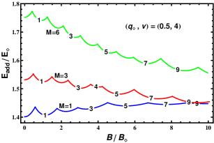
Figure 5: The additional energies for different potentials with $M\hskip-1.5pt=\hskip-1.5pt1,3,6$. See text.

In order to compare results for different potentials, we will study a sequence of lists ${\mathsf{l}}_{k}$ obtained by choosing a few values $M_{k}$, $M_{1}\hskip-1.5pt=\hskip-1.5pt1$ and $G_{7}$ action: ${\mathsf{l}}_{k}\hskip-1.5pt=\hskip-1.5ptg_{M_{k}}\cdot{\mathsf{l}}_{1}$ (see Eqs.(88,89)). Since, the mathematical model is constructed with the aid of parameters ${\mathsf{k}}$, we have: ${\mathsf{k}}_{k}=\hat{g}_{M}\cdot{\mathsf{k}}_{1}$.

This trick enables to us to trace the evolution of harmonic quantum effects with the increase of the magnetic field for different potentials on the same figure. We consider the same parabolic confinement potential with $v=\omega_{z}/\omega_{\rho}\hskip-1.5pt=\hskip-1.5pt4$, when the quantum contribution is by twice smaller than the classical contribution $q_{\diamond}=0.5$. The result are displayed on Fig. 5. For a better visualization, the additional energies $E_{\rm add}$ (a vertical axis) have been multiplied by the factor $g_{M}\!:g_{M}\hskip-1.5pt=\hskip-1.5pt\hskip-1.5pt=\hskip-1.5pt3/(1+M/2)$ ($g_{1}\hskip-1.5pt=\hskip-1.5pt1$) resulting from the formula of minimal states: $\mbox{\rsfs E}_{\,\rm rel}=\tfrac{1}{2}\,(1+M/2),\,1<v$ (see Eq.(66)).

The effect of vibrations is most visible for the potential with the larger $M$. Indeed, the deeper is the potential, the larger is the amplitude of vibrations. The magnetic field diminishes quantum fluctuations. The potentials with $M=1,3$ tend asymptotically to the classical limit $\sim 3/2$ at large magnetic fields, while the quantum fluctuations are still strong for the potential with $M=6$. Thus, the developed model provides a relatively simple way to analyse a full 3D-dynamics of two fermions interacting by means of the potential $\mbox{\rsfs U}_{M}({\mathsf{r}})=\alpha_{M}\,r^{-M}\,(\alpha_{M}>0,M>0)$ under the perpendicular magnetic field.

VI Summary

We formulated the algebraic approach in order to study classical and quantum correlations in two-fermion systems confined by the 3D axially-symmetric parabolic potential in the harmonic approximation. The system dynamics is governed by the interplay between the two-body interaction in the form $\mbox{\rsfs U}_{M}({\mathsf{r}})\hskip-1.5pt=\hskip-1.5pt\alpha_{M}\,r^{-M}(\alpha_{M}>0,M>0)$, the confinement potential and the external magnetic field. For this problem we suggest the scaling symmetry $G_{4}$. Since the latter acts effectively on the parameters $(B,m{{}_{\ast}})$, this symmetry enables one to establish a similarity between results obtained for system Hamiltonians with different efective masses $m{{}_{\ast}}$. It would be desirable to test the validity of this symmetry in experiments with real QDs.

The analytical results, obtained in the harmonic approximation, provide a reliable description of the evolution of the ground and excited states of two-fermion systems in the applied magnetic field. The harmonic approximation is well justified when the classical correlations dominate over quantum ones. The validity of our approach have been proved by a remarkable agreement with numerical results for QDs parameters available in experiments nen3 .

Our analysis reveals the coexistence of different shapes which under certain conditions may transform from one to another. Indeed, the interplay between classical and quantum correlations may lead to a shape transition from a lateral to a vertical localization of the confined electrons due to diminishing of quantum fluctuations under certain choice of the system parameters. Such a transition is accompanied by a spontaneous symmetry breaking of the inner parity symmetry $\mbox{\rsfs P}_{\rm in}$ at the preserved integral of motion $p_{\varphi}=$const. This general result is nicely supported by exact numerical calculations for the case of the Coulomb interaction ent ; PR .

Appendix A The explicit $(u,p_{\varphi})$-representation of ${\mathsf{S}}$ states

In order to find a general solution of Eq.(59) for an arbitrary value $M$ we recall that: i) the family ${\mathsf{A}}$ states is subject to the condition (44); ii) the border line for the onset of the family maximal ${\mathsf{A}}_{u,v}$ states is defined by Definition 1. These conditions lead to the conclusion that the function $v{{}_{\ast}}$ obeys the inequality $v{{}_{\ast}}^{2}<1+u^{2}$ for all values $u,\,p_{\varphi}$ identically. To proceed further let us to introduce the following notations

$$y_{u}=\frac{v{{}_{\ast}}}{\sqrt{1+u^{2}}},\qquad P_{\alpha}(z)=z^{\alpha}.$$ (91)

In virtue of these definitions, Eq.(59) can written in the following form

$$\frac{p_{\varphi}}{b_{M}(u)}=P_{1/(2\,a)}\circ F_{a}\circ P_{2}(y_{u}),$$ (92)

where

$$F_{a}(y)=y\,(1-y)^{a},\quad a=-(M+2)/4,\quad b_{M}(u)\hskip-1.5pt=\hskip-1.5pth_{M,2}\times h_{M,(M-2)/2}(1+u^{2}).$$ (93)

Let us precede the analysis of Eq.(92) by the discussion of some symmetry of $F$ identifying $F$ with $\tilde{F}(a,y)\hskip-1.5pt=\hskip-1.5pt(a,F_{a}(y))$ and assuming that $(a,y)\in\mathbb{R}_{+}\otimes[0,1]=D$. Let $\tilde{f}^{\pm}(a,y)=(a,f_{\pm}(a,y))$ and $\phi$ be transformation $\phi:\tilde{f}^{\pm}\to\tilde{f}^{\mp}$ given by $\tilde{f}^{\mp}(a,y)\hskip-1.5pt=\hskip-1.5pt\phi(\tilde{f}^{\pm})(a,y)\hskip-1.5pt=\hskip-1.5pt(a,f_{\pm}{{}^{a}}(1/a,1-y))$; hence if $f_{\pm}(a,y)\in\mathbb{R}_{+}$ then $\tilde{f}^{\pm}\hskip-1.5pt=\hskip-1.5pt\phi(\tilde{f}^{\mp})\hskip-1.5pt=\hskip-1.5pt\phi\circ\phi(\tilde{f}^{\pm})$. Since $\phi(\tilde{F})\hskip-1.5pt=\hskip-1.5pt\tilde{F}$, so $\phi$ is the symmetry. The transformation $\phi$ decomposes: $\phi(\tilde{f})\hskip-1.5pt=\hskip-1.5ptP\circ\tilde{f}\circ R$, where $P(a,y)\hskip-1.5pt=\hskip-1.5pt(1/a,y^{1/a})$, $R(a,y)\hskip-1.5pt=\hskip-1.5pt(1/a,1-y)$ and $P\circ P\hskip-1.5pt=\hskip-1.5ptR\circ R={\rm id}_{D}$; hence, inverting both sides of equation $\tilde{F}_{\mp}\hskip-1.5pt=\hskip-1.5pt\phi(\tilde{F}_{\pm}),\,(\tilde{F}_{+}\hskip-1.5pt\equiv\hskip-1.5pt\tilde{F}_{-})$, one finds

$$\tilde{G}^{\mp}=\phi{{}_{\ast}}(\tilde{G}^{\pm})=R\circ\tilde{G}^{\pm}\circ P\,,$$ (94)

where $\tilde{F}^{\mu}\circ\tilde{G}^{\mu}={\rm id}_{D}$. With the aid of the original notations Eq.(94) transforms to the form

$$G^{\mp}_{a}(x)=(\phi{{}_{\ast}}(G^{\pm}))_{a}(x)=1-G^{\pm}_{1/a}{{}^{1/a}}(x)\,.$$ (95)

The geometric interpretation of components $G^{\pm}_{a}$ is obtained, taking into account that the derivative $F^{\prime}$ vanishes at a point $\hat{y}_{a}\in[0,1]$; hence $\hat{x}_{a}=F_{a}(\hat{y}_{a})={\rm max}_{y\in[0,1]}F_{a}(y)$. It proves that the inverse of $F$ is determined as the doubly valued function $(G^{-}_{a},G^{+}_{a})$ defined on the interval $[0,\hat{x}_{a}]$. In order to pass to a single valued one, let $F^{\mu}_{a}\in{\rm Map}(Y_{\mu},\mathbb{R}_{+})$, where $Y_{-}=[0,\hat{y}_{a}]$, $Y_{+}=[\hat{y}_{a},1]$. As a result, $F^{\pm}_{a}$ represent two monotonic functions, and, if $G^{\mu}\circ F^{\mu}_{a}={\rm id}_{\rm Y_{\mu}}$, then

$$G^{-}_{a}(0)=0,\qquad G^{+}_{a}(0)=1,\qquad G^{\pm}_{a}(\hat{x}_{a})=\hat{y}^{a}.$$

Note, that Eq.(59) is determined as the inversion of the function on the right hand side of Eq.(92). It has the following form:

$$v_{\ast}(p_{\varphi},u,M)=\sqrt{1+u^{2}}\,P_{a}\circ G^{-}_{a}\circ P_{2\,a}(p_{\varphi}/b_{M}(u)).$$ (96)

Applying $$G^{-}_{a}\hskip-1.5pt=\hskip-1.5pt\phi{{}_{\ast}}(G^{+})$$ (see also Eq.(95)), one obtains

$$v_{\ast}(p_{\varphi},u,M)=\sqrt{1+u^{2}}\times[1-G^{+}_{1/a}\circ\bar{x}(p_{\varphi})]^{1/2},$$ (97)

$$\bar{x}(p_{\varphi})\hskip-1.5pt=\hskip-1.5pt[(p_{\varphi}/b_{M}(u))^{2\,a}]^{1/a}=(p_{\varphi}/b_{M}(u))^{2}<\hat{x}_{a}{{}^{1/(2\,a)}}.$$ (98)

where the parameter $a$ depends on $M$, in the accordance with Eq.(93). In the physical case $-2<M\Rightarrow a<0$.

Consider the implication $\hat{x}_{a}{{}^{1/(2\,a)}}\hskip-1.5pt<\hskip-1.5ptz_{u}$ then $x=P_{2\,a}(z_{u})\in[\hat{x}_{a},1]$ else $x\in[0,\hat{x}_{a}]$ ($a<0)$, where $z_{u}\hskip-1.5pt=\hskip-1.5ptp_{\varphi}/b_{M}(u)$. The equation (96) expresses the result of summation of Taylor series for $v{{}_{\ast}}$ in powers of $1/z_{u}$ (i.e., for the expansion at $z_{u}=\infty$). Taking Eq.(98) in the limit $z_{u}{{}^{2}}-1=\bar{x}(p_{\varphi})-1\to 0^{+}$, one observes that Eq.(97) provides the result of summation of the Taylor series for $v{{}_{\ast}}$ in powers of $z_{u}-1$, i.e., when $b_{M}(u)\leq p_{\varphi}\ll 2\,b_{M}(u)$.

Since Eqs.(96),(97), are analytically conjugated by means of the symmetry $\phi$, we have to calculate the function $G^{-}_{a}(x)$ explicitly. Taking into account that coefficients $a_{k}$ of the expansion of series $F_{a}(y)\hskip-1.5pt=\hskip-1.5pt\Sigma_{1\leq k}\,a_{k}\,y^{k}$ at the point $y\hskip-1.5pt=\hskip-1.5pt0$ are known, we conclude that the function $G^{-}_{a}(x)$ can be obtained by means of the summation of the inverse series $G^{-}_{a}(x)\hskip-1.5pt=\hskip-1.5pt\Sigma_{1\leq k}\,a^{\ast}_{k}\,y^{k}$. Following this way, let us write

$$y\equiv G^{-}_{a}\circ F^{-}_{a}(y)=\Sigma_{1\leq k}\,a^{\ast}_{k}\,(\Sigma_{1\leq m}a_{m}\,y^{m})^{k}=\Sigma_{1\leq p}\,(\Sigma_{1\leq k\leq p}\,a^{\ast}_{k}\,d_{[a_{1},\ldots],k,p})\,y^{p},$$ (99)

where the coefficients $d_{[{\mathsf{a}}],k_{1},k}$ are defined by means of the relation $(\Sigma_{1\leq m}a_{m}\,x^{m})^{k_{1}}\hskip-1.5pt=\hskip-1.5pt\Sigma_{1\leq p}\,d_{[{\mathsf{a}}],k_{1},k}\,x^{k}$. Let $\{k_{1},k_{2},\ldots,k_{r}\}\in S_{k}$ be a partition of number $k\equiv\Sigma_{i}k_{i}$ (an irreducible representation of the symmetric group $S_{k}$). With the aid of such a partition we determine the coefficients $d_{[{\mathsf{c}}],l,k}$ as

$$d_{[{\mathsf{c}}],l,k}=l!\times\mbox{$\sum\limits_{{\mathsf{k}}\in S_{k}|k_{1}=l}$}\;\mbox{$\prod\limits_{i\leq k}$}\,c_{i}{{}^{\Delta k_{i}}}/(\Delta k_{i})!,\qquad\Delta k_{i}=k_{i}-k_{i+1}\geq 0,\;k_{k+1}\equiv 0.$$ (100)

Here, $\Sigma_{{\mathsf{k}}\in S_{k}|k_{1}=l}$ is a sum over irreducible representations of the group $S_{k}$ in which the first member $k_{1}$ of ${\mathsf{k}}$ is fixed $k_{1}\hskip-1.5pt=\hskip-1.5ptl$. It constrains the summation over the irreducible representations of the group: $S_{k}\to S_{k-k_{1}}$.

The summation $\Sigma_{{\mathsf{k}}\in S_{k}|k_{1}}f({\mathsf{k}})$ is easy to perform by means of the operator $d_{k}.$ Such an operator can be defined as follow: ${\mathsf{k}}_{i+1}\hskip-1.5pt=\hskip-1.5ptd({\mathsf{k}})_{i},\,{\mathsf{k}}_{i}\in S_{k}$ obtained with the aid of the following ordering of partitions:

$$\{m_{1}\ldots m_{s}\}\hskip-1.5pt<\hskip-1.5pt\{k_{1}\ldots k_{r}\}\Leftrightarrow s\leq r\vee(r=s)\wedge(m_{s}\hskip-1.5pt<\hskip-1.5ptk_{s}\vee m_{s}=k_{s}\wedge(\ldots\vee(m_{2}<k_{2})\ldots)).$$

The sequence generated by $d$ determines a list: $\{\{k_{1}k\hskip-1.5pt-\hskip-1.5ptk_{1}\},\{k_{1}k\hskip-1.5pt-\hskip-1.5ptk_{1}-1\,1\},\ldots,\{k_{1}1^{k-k_{1}}\}\}$. Evidently, the constraint $k_{1}\hskip-1.5pt=\hskip-1.5pt{\rm const}$ is consistent with the applied ordering, which makes this list to be complete.

Eq.(100) is valid, if $c_{i}\hskip-1.5pt\neq\hskip-1.5pt0$. Contrary, if $c_{l_{1}}\hskip-1.5pt=\hskip-1.5ptc_{l_{2}}=\ldots\hskip-1.5pt=\hskip-1.5pt0$, we have to put $\Delta k_{l_{1}}=\Delta k_{l_{2}}\hskip-1.5pt=\hskip-1.5pt\ldots\hskip-1.5pt=\hskip-1.5pt0\Rightarrow c_{i}{{}^{\Delta k_{i}}}/(\Delta k_{i})!\hskip-1.5pt=\hskip-1.5pt1$; hence, the elements $i\hskip-1.5pt=\hskip-1.5ptl_{1},l_{2},\ldots$ do not contribute to the considered product. For $p=1$ in Eq.(99) $a^{\ast}_{1}\,a_{1}\hskip-1.5pt=\hskip-1.5pt1\Rightarrow a^{\ast}_{1}=1/a_{1}$. Taking into that $d_{[{\mathsf{a}}],k,k}\hskip-1.5pt=\hskip-1.5pta_{1}{{}^{k}}$ (we applied: $\Sigma_{{\mathsf{k}}\in S_{k}}\hskip-1.5pt=\hskip-1.5pt\{k,0,\ldots,0\})$ and the relation (100), we find a recurrent algorithm

$$a^{\ast}_{i+1}\hskip-1.5pt=\hskip-1.5pt\psi_{i}(a_{1},\ldots,a_{i}),\qquad\psi_{i}(a_{1},\ldots,a_{i})\hskip-1.5pt=\hskip-1.5pt-a_{1}{{}^{-i-1}}\,\Sigma_{m\leq i}\,a^{\ast}_{m}\,d_{[a_{1},\ldots],m,i+1},$$ (101)

for the calculation of the coefficients ${\mathsf{a}}^{\ast}$. Employing this recurrent relations for coefficients $a_{k}$ of series $F_{a}(y)$: $a_{k}\hskip-1.5pt=\hskip-1.5pt(-1)^{k-1}\tbinom{a}{k-1}$ one finds

$$G^{-}_{a}(x)=\mbox{$\sum\limits_{k=1}^{\infty}$}\,{a^{\ast}_{k}}\,x^{k}\hskip-1.5pt=\hskip-1.5ptx+a\,\mbox{$\sum\limits_{k=2}^{\infty}$}\,\frac{(t)_{k-2}}{(k-1)!}\,(-x)^{k},\qquad t=2-k\,(a+1),$$ (102)

where $(t)_{k}$ is a Pochhammer symbol.

In some cases the series $G^{-}_{a}$ and $G^{+}_{a}$ studied with aid of the recurrence (101) can be analytically summed, which yields the explicit equivalence of Eqs.(96),(97). Most simple form of $G_{M,-}(x)\hskip-1.5pt\equiv\hskip-1.5ptG^{-}_{a(M)}(x)$ ($G_{M,+}\hskip-1.5pt\equiv\hskip-1.5ptG^{+}_{1/a(M)}(x))$ applied in Eqs.(96) (Eq.(97)) for $a\hskip-1.5pt\equiv\hskip-1.5pta(M)$ given in Eq.(93) are found in the following cases:

$$G_{2,-}=(1+x)^{-1}\,x,\qquad G_{6,-}\hskip-1.5pt=\hskip-1.5pt(2\,x)^{-1}\,(1+2x-\sqrt{1+4\,x}),$$

$$G_{2+\,4\,k,-}(x)=1-{}_{k}{\rm F}_{k-1}(\tfrac{1}{k+1},\tfrac{2}{k+1},\ldots,\tfrac{k}{k+1};\,\tfrac{2}{k},\ldots,\tfrac{k-1}{k},\tfrac{k+1}{k};\,x),\qquad k=2,3,\ldots\,,$$ (103)

where ${}_{k}{\rm F}_{k-1}$ are generalized hypergeometric functions. In particular, for $k\hskip-1.5pt=\hskip-1.5pt2$ Eq.(103) reduces to the form $G_{10,-}(x)=1-(2/\sqrt{3\,x})\,\sinh{\tfrac{1}{3}\,{\rm arcsinh}\,(\sqrt{27\,x}/2)}$.

References

- (1) Cejnar P, Jolie J, Casten R F 2010 Rev. Mod. Phys. 82, 2155
- (2) Kresin V Z, Ovchinikov Y N, Wolf S A 2006 Phys. Rep. 431, 231
- (3) Sachdev S 2011 Quantum Phase Transitions (Cambridge: Cambridge University Press) 2nd Edition
- (4) Kais S, Herschbach D R, Levine R D 1989 J. Chem. Phys. 91, 7791
- (5) Taut M 1994 J. Phys. A: Math. Gen. 27, 1045
- (6) Dineykhan M, Nazmitdinov R G 1997 Phys. Rev. B 55, 13707
-
(7)
Nazmitdinov R G, Simonović N S, Plastino A, Chizhov A V 2012
J. Phys. B: At. Mol. Opt. Phys. 45, 205503 - (8) Ashoori R C, Stormer H L, Weiner J S, Pfeiffer L N, Baldwin K W, West K W 1993 Phys. Rev. Lett. 71, 613
- (9) Kouwenhoven L P, Austing D G, Tarucha S 2001 Rep. Prog. Phys. 64, 701
- (10) Reimann S M, Manninen M 2002 Rev. Mod. Phys. 74, 1283
- (11) Nazmitdinov R G 2009 Physics of Particles and Nuclei 40, 71
- (12) Birman J L, Nazmitdinov R G, Yukalov V I 2013 Physics Reports 526 1
- (13) Lozovik Yu E, Mur V D, Narozhnyi N B 2003 Zh. Eksp. Teor. Fiz. 123, 1059 [JETP 96, 932 (2003)]
- (14) Kandemir B S 2005 J. Math. Phys. 46, 032110
- (15) Grossmann F, Kramer T 2011 J. Phys. A: Math. Theor. 44, 445309
- (16) Nishi Y, Tokura Y, Gupta J, Austing G, Tarucha S 2007 Phys. Rev. B 75, 121301(R)
- (17) Rontani M, Rossi F, Manghi F, Molinari E 1999 Phys. Rev. B 59, 10165
- (18) Bruce N A, Maksym P A 2000 Phys. Rev. B 61, 4718
- (19) Nazmitdinov R G, Simonović N S 2007 Phys. Rev. B 76, 193306
- (20) Simonović N S, Nazmitdinov R G 2008 Phys. Rev. A 78, 032115
- (21) Arnol’d V I 1989 Mathematical Methods of Classical Mechanics (Berlin: Springer)