Physical characterization of quantum devices from nonlocal correlations

Abstract

In the device-independent approach to quantum information theory, quantum systems are regarded as black boxes which, given an input (the measurement setting), return an output (the measurement result). These boxes are then treated regardless of their actual internal working. In this paper, we develop SWAP, a theoretical concept which, in combination with the tool of semi-definite methods for the characterization of quantum correlations, allows us to estimate physical properties of the black boxes from the observed measurement statistics. We find that the SWAP tool provides bounds orders of magnitude better than previously-known techniques (e.g.: for a CHSH violation larger than 2.57, SWAP predicts a singlet fidelity greater than $70\%$). This method also allows us to deal with hitherto intractable cases such as robust device-independent self-testing of non-maximally entangled two-qutrit states in the CGLMP scenario (for which Jordan’s Lemma does not apply) and the device-independent certification of entangled measurements. We further apply the SWAP method to relate nonlocal correlations to work extraction and quantum dimensionality, hence demonstrating that this tool can be used to study a wide variety of properties relying on the sole knowledge of accessible statistics.

I Introduction

In the last few years, several tasks for which quantum physics offers an advantage over classical methods have been found possible without assuming knowledge of the inner working of the devices involved, i.e. in a device-independent manner. This is the case of key distribution qkd1 ; qkd2 ; qkd3 ; qkd4 ; qkd5 and randomness certification random1 ; random2 for instance (see also review ; slovakia and references therein for more examples).

In a device-independent experiment, also known as a Bell-type experiment, conclusions are not drawn from the knowledge that specific resources are used by the devices – the content of the devices might not be known a priori –, but only from the observed relation between their inputs and outputs. Therefore, such devices are referred to as black boxes. Any actual physical realization of black boxes providing an advantage over classical devices must however use some quantum resource. For instance, the violation of a bipartite Bell inequality requires two black boxes to share an entangled quantum state. Some knowledge about the underlying quantum state can thus be inferred from the observed correlations only.

Several works have shown that, beyond the mere presence of entanglement, other quantum features such as genuine entanglement bancal11 , the dimension of the underlying Hilbert space brunner08 , or the overlap between measurements tomamichel13 can also be witnessed from correlations only. Moreover, quantitative statements have also been obtained, for instance on the amount of entanglement bardyn ; moroder . But even quantifying these aspects never fully characterizes the underlying quantum realization: several states have the same negativity or Hilbert space dimension, and several sets of measurements can have the same overlap. In fact, all of these estimations could be deduced if one were able to identify which states and measurements are performed by the black boxes in the first place. This is the subject of this paper (see Figure 1).

The question of identifying quantum states and measurements from correlations only was originally addressed in two inequivalent ways. The first criterion is due to Refs. Tsirelson93 ; sw87 ; pr92 , where it is shown that if the Clauser-Horne-Shimony-Holt (CHSH) inequality chsh is violated maximally (given by the famous value of $2\sqrt{2}$ tsirelson ), then the state being measured is equivalent to a maximally entangled state and the measurements are anti-commuting on both Alice’s and Bob’s part. Another criterion that certifies the same state and measurements is due to Mayers and Yao yao (see also werner ).

These pioneering works showed that there exist lists of statistical data in the device-independent framework which allow one to identify the quantum state and measurement operators involved in the actual experiment. Moreover, the process can tolerate a small amount of external noise. This notion of determining approximately the state and measurement operators involved via non-locality detection is known as device-independent self-testing (or simply self-testing for short), and it has inspired a number of works on the subject st1 ; mckague ; miller ; reichardt ; yang .

However, the weak noise tolerance exhibited by the self-testing protocols proposed so far makes them inapplicable in realistic experimental situations. Moreover, all of them are specific to a given Bell inequality st1 ; mckague ; reichardt , or family of Bell inequalities yang , and thus cannot be applied to arbitrary states or measurements.

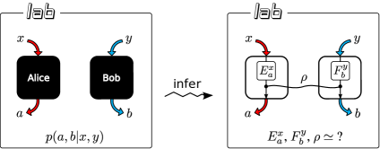
Figure 1: We are interested in certifying the physical properties of black boxes. This amounts to question the nature of the underlying quantum state $\rho$ and of the measurement operators $E^{x}_{a}$, $F^{y}_{b}$ which are necessary for some boxes to produce the observed statistics $p(a,b|x,y)$.

In this paper, building on the method sketched in Ref. yang_prl , we present the SWAP method, a unified tool that allows one to guess the state, measurements or other general properties of the quantum systems inside the boxes from the experimentally accessible correlations. The process is algorithmic, i.e., it is completely automated, and makes use of the Navascués-Pironio-Acín (NPA) hierarchy for the characterization of quantum correlations navascues . To illustrate the power of this method, we apply it to estimate different physical properties in standard Bell scenarios.

The structure of this paper is as follows. First, we recall the formal definition of self-testing. Next, in Section III, we explain the main idea behind our method: an effective description, in the language of moment matrices, of the process of exchanging the content of black boxes with a trusted finite-dimensional system. This idea, together with the NPA hierarchy navascues ; navascueslong , allows us to estimate quantum monotones via convex optimization convex , in the same way that we would calculate such monotones had we known the exact mathematical representation of the state and measurement operators involved in the non-locality experiment. We also indicate in this section how our results can be easily generalized to the case where black boxes are not independently and identically distributed (i.i.d.). In Section IV, we demonstrate that the method improves the noise tolerance of previous self-testing protocols by several orders of magnitude. Next, we show how the method can be applied to Bell-type scenarios for which, due to their complexity, no robust device-independent protocols (no matter how fragile to noise) could be derived before. These are: self-testing of states with measurements having more than two possible outcomes (Section V.1); the certification of entangled measurements (Section V.2); and the estimation of the amount of work extractable from non-local quantum systems (Section V.3).

II Self-testing

Let Alice and Bob be two distant observers conducting measurements on a shared quantum system. If Alice (Bob) makes no assumption on the inner mechanisms of their experimental devices, she (he) has to regard each of her (his) device as a black box where she (he) inputs a symbol $x$ ($y$) – the measurement setting – and obtains an output $a$ ($b$) – the measurement outcome. In these conditions, Alice and Bob can make a frequency analysis to estimate $p(a,b|x,y)$, the probability that they observe results $a,b$ when they input $x,y$. The question of self-testing is whether the user can deduce, from the knowledge of these conditional probabilities only, the state and measurements used inside their boxes (see Figure 1).

According to quantum theory, there exist a state $\rho$ and measurement operators $\{E^{x}_{a},F^{y}_{b}\}$ such that $p(a,b|x,y)=\mbox{tr}(\rho\,E^{x}_{a}\otimes F^{y}_{b})$. Assuming that all physical implementations of a Positive Operator Valued Measure (POVM) involve a projective measurement over a dilated space, the operators $\{E^{x}_{a},F^{y}_{b}\}$ can be taken as projectors. The underlying quantum state $\rho$ to which both parties have access in their labs can, in principle, be mixed. For simplicity, for all subsequent discussions, we will take it to be pure, i.e., $\rho=|\Psi\rangle\!\langle\Psi|$. However, as the reader can appreciate, all results presented in this paper hold independently of this assumption.

Now, suppose that, after many runs of an experiment, the parties observe a probability distribution that is compatible with some specific state and measurements $(|\overline{\psi}\rangle,\{\overline{E}^{x}_{a},\overline{F}^{y}_{b}\})$ defined in ${\mathbb{C}}^{d}\otimes{\mathbb{C}}^{d}$:

$$p(a,b|x,y)=\langle\overline{\psi}|\overline{E}^{x}_{a}\otimes\overline{F}^{y}_{b}|\overline{\psi}\rangle.$$ (1)

In general, this observation does not imply that the actual state $|\psi\rangle$ and measurements $\{E^{x}_{a},F^{y}_{b}\}$ used by the black boxes are these ones: since correlation admit in general several possible quantum realizations, the actual states and measurements could be different. Remarkably, however, for some $p(a,b|x,y)$ it turns out that the guessed state and measurements $(|\overline{\psi}\rangle,\{\overline{E}^{x}_{a},\overline{F}^{y}_{b}\})$ are the only possible ones, up to local unitaries and the addition of irrelevant degrees of freedom. In this case, the observation of $p(a,b|x,y)$ certifies that the states and measurements used by the boxes are the guessed ones.

Technically, this is captured by the following self-testing statement: the correlations $p(a,b|x,y)$ allow for self-testing if for every quantum realization $(|\psi\rangle,\{E^{x}_{a},F^{y}_{b}\})$ compatible with $p(a,b|x,y)$ there exists a local isometry $\mathbf{\Phi}=\mathbf{\Phi}_{A}\otimes\mathbf{\Phi}_{B}$ such that

$$\mathbf{\Phi}|\psi\rangle = |\overline{\psi}\rangle_{A^{\prime}B^{\prime}}\otimes|\textrm{junk}\rangle_{AB}$$ (2)

$$\mathbf{\Phi}(E^{x}_{a}\otimes F^{y}_{b}|\psi\rangle) = (\overline{E}^{x}_{a}\otimes\overline{F}^{y}_{b}|\overline{\psi}\rangle)_{A^{\prime}B^{\prime}}\otimes|\textrm{junk}\rangle_{AB}$$ (3)

where $A^{\prime}$ and $B^{\prime}$ are two ancillary qudits. The isometry must be seen as a virtual protocol: it does not need to be implemented in the lab as part of the procedure of self-testing, all that must be done in the lab is to query the boxes and derive $p(a,b|x,y)$.

Intuitively, the isometry consists of local swaps that put the relevant degrees of freedom from the boxes into the ancillas, which have the right dimension for a comparison with the desired state and measurement to be possible. Indeed, the intuition of the swap was already mentioned in the work of Mayers and Yao yao . However, it was not exploited to derive a general method as we are going to do here.

III The method

We first present the SWAP method with a specific example and then show how a general construction is possible for any self-testing scenario. Finally we show how to remove the assumptions of infinitely many runs and the assumption that the behavior of the devices is the same in each run and uncorrelated among the runs (the latter being usually called i.i.d. assumption by analogy with sampling of probability distributions).

III.1 Example: self-testing of qubit states

III.1.1 Construction of the swap operator

Since the swaps are local operations, it is enough to show how to construct one for Alice (the same construction applies to the other parties). In case the state we wish to self-test is a qubit state, the local ancilla $A^{\prime}$ is a qubit. To construct the swap, we start by temporarily assuming that the state inside the box is indeed a qubit, and then relax this assumption.

In case the state inside Alice’s box is a qubit, the swap operator between her system and ancilla can be written as the concatenation of three CNOT gates with alternate controls:

$${\cal S}_{AA^{\prime}} = UVU\,,$$ (4)

where

$$\begin{array}[]{lcl}U&=&\mathbb{I}\otimes|0\rangle\langle 0|+\sigma_{x}\otimes|1\rangle\langle 1|\\ V&=&|0\rangle\langle 0|\otimes\mathbb{I}+|1\rangle\langle 1|\otimes\sigma_{x}\end{array}$$ (5)

are the CNOT gates with the ancilla, respectively the system, as control.

For simplicity, in this introduction we assume further that the operators $\sigma_{z}$ and $\sigma_{x}$ are part of the set of operators we want to self-test (see Section IV.4 for an example when this is not the case). For instance,

$$\sigma_{z} = \overline{A}_{0}\,\equiv\,\overline{E}^{0}_{a=+1}-\overline{E}^{0}_{a=-1}$$ (6)

$$\sigma_{x} = \overline{A}_{1}\,\equiv\,\overline{E}^{1}_{a=+1}-\overline{E}^{1}_{a=-1}\,.$$ (7)

The trick is now to rewrite $U$ and $V$ with $\overline{A}_{0}$ and $\overline{A}_{1}$ on the side of the system, then to replace them by the real $A_{0}$ and $A_{1}$ operators defined analogously from the actual projectors $E^{x}_{a}$. This gives

$$\begin{array}[]{lcl}U&=&\mathbb{I}\otimes|0\rangle\langle 0|+A_{1}\otimes|1\rangle\langle 1|\\ V&=&\frac{\mathbb{I}+A_{0}}{2}\otimes\mathbb{I}+\frac{\mathbb{I}-A_{0}}{2}\otimes\sigma_{x}\,.\end{array}$$ (8)

At this point, we have dropped the requirement that the system is a qubit. Nevertheless, these two operators are still unitary, because, by assumption, $A_{x}^{2}=\mathbb{I}$. Finally, the guess for the swap operator is just (4) with the new expressions (8) for $U$ and $V$.

Using the same construction for Bob’s side, the final guess for the swap operator is

$${\cal S} = {\cal S}_{AA^{\prime}}\otimes{\cal S}_{BB^{\prime}}\,.$$ (9)

A few remarks are in order here. First, note that ${\cal S}_{AA^{\prime}}=VUV$ would be an equally valid choice instead of (4). However, in several situations it can be preferable to use (4). For instance, if the ancilla is initialized in the state $|0\rangle$, then the action of the first $U$ is equivalent to the identity. $\mathcal{S}_{AA^{\prime}}$ then reduces to $UV$, which leads to simpler numerical computations than $VUV$. We refer to $UV$ as a partial swap.

Second, note that the swap defined here explicitly depends on the measurement operators used by the individual parties. This guarantees that the result of applying this swap to the measured state is identical for all unitarily equivalent quantum representations.

III.1.2 State certification with the SDP hierarchy

Once the swap operator is defined, the next step of the method describes how to use the knowledge of the correlations $p(a,b|x,y)$.

For this, consider the self-testing of the state (2); the self-testing of measurements (3) follows a similar path and will be sufficiently illustrated by our example in Section IV.3. A possible figure of merit is the fidelity

$$F = \langle\overline{\psi}|\rho_{\text{swap}}|\overline{\psi}\rangle$$ (10)

where $\rho_{\text{swap}}$ is the state of the ancillas after the swap. The relation between this figure of merit and the trace-distance between the desired and actual states is discussed in Section IV.1.

Explicitly, if the initial dummy states of the ancillas are denoted by $\rho_{A^{\prime}}$ and $\rho_{B^{\prime}}$, we have

$$\rho_{\text{swap}}=\mbox{tr}_{AB}\left[{\cal S}\,(|\psi\rangle\langle\psi|)_{AB}\otimes\rho_{A^{\prime}}\otimes\rho_{B^{\prime}}\,{\cal S}^{\dagger}\right]\,,$$ (11)

where the SWAP operator ${\cal S}$ is defined by Eq. (9). Having expressed ${\cal S}$ in terms of four of the desired operators $A_{0}$, $A_{1}$, $B_{0}$ and $B_{1}$, we find $\rho_{\text{swap}}$ to be a $4\times 4$ matrix whose entries are linear combinations of expectation values like $\langle\psi|A_{x}\otimes\mathbb{I}|\psi\rangle$, $\langle\psi|A_{0}A_{1}\otimes\mathbb{I}|\psi\rangle$, $\langle\psi|A_{x}\otimes B_{y}|\psi\rangle$, etc. Consequently, our estimate $f$ on the singlet fidelity $F$ attainable via isometries (10) is a linear combination of operator averages of the form $c_{t}=\langle\psi|t(A_{x},B_{y})|\psi\rangle$, where $t$ is a product of the operators $A_{x},B_{y}$.

Self-testing is perfect, i.e. (2) holds exactly, if we find $f=1$; but the method automatically deals with imperfect cases, that is, it is robust by construction. So we are finally left to estimate the minimal possible value of $f$ compatible with $p(a,b|x,y)$ and with quantum physics. In other words, we must solve the problem

$$\underset{d}{\min}\;\; f({d})=\langle\overline{\psi}|\rho_{\mathrm{swap}}({d})|\overline{\psi}\rangle$$

s.t. $${d}\in{\cal Q}$$

$$\frac{1}{4}\left\{1+(-1)^{a}{d}_{A_{x}}+(-1)^{b}{d}_{B_{y}}\right.$$

$$\ \ \left.+\ (-1)^{a+b}{d}_{A_{x}B_{y}}\right\}=p(a,b|x,y).$$ (12)

where the maximization ${d}\in{\cal Q}$ is performed over the set ${\cal Q}$ of all vectors ${d}=({d}_{\mathbb{I}},{d}_{A_{0}},...)$ that admit a quantum representation, i.e., for which there exists a state $|\psi\rangle$ and dichotomic operators $A_{x},B_{y}$ such that ${d}_{t}=\langle\psi|t(A_{x},B_{y})|\psi\rangle$ for all products $t$. Note that in the optimization problem above we assumed for simplicity a probability distribution $p(a,b|x,y)$ with dichotomic settings, $a,b\in\{0,1\}$.

Optimizations over the set of quantum momenta are computationally hard ito , and, in some scenarios, conjectured to be undecidable tobias . That is why we propose to relax the above problem to an optimization over the sets ${\cal Q}^{S}$, defined in navascues as outer approximations of the quantum set. Let $S$ be a set of products of the operators $A_{x},B_{y}$, and let ${d}$ be a complex vector whose entries are labeled by products of the form $s^{\dagger}t$, with $s,t\in S$ (objects such as ${d}$ will be called moment vectors). We define $\Gamma^{S}({d})$ as a matrix whose rows and columns are numbered by products belonging to $S$ and such that $\Gamma_{s,t}={d}_{s^{\dagger}t}$. It can be shown that ${d}\in{\cal Q}$ implies that $\Gamma^{S}({d})$ is positive semidefinite. The relaxation we propose to attack problem (12) is thus:

$$f^{S}=\underset{d}{\min}\;\; f({d})$$

s.t. $$\Gamma^{S}({d})\geq 0$$

$$\frac{1}{4}\left\{1+(-1)^{a}{d}_{A_{x}}+(-1)^{b}{d}_{B_{y}}+\right.$$

$$\ \ \left.+\ (-1)^{a+b}{d}_{A_{x}B_{y}}\right\}=p(a,b|x,y).$$ (13)

This last problem can be formulated as a semidefinite program (SDP) convex , a type of convex optimization for which there exist efficient numerical solvers to find global minima and which also return sound error bounds on the optimal guess. A note on notation: whenever $S$ corresponds to the set of all products of $n$ or less measurement operators, we will denote the corresponding set ${\cal Q}^{S}$ as ${\cal Q}^{n}$. It can be verified that, if certain conjectures in von Neumann algebras hold ozawa , the sequence of sets $({\cal Q}^{n})_{n}$ converges to ${\cal Q}$ navascueslong .

We stress that the bound on $F$ obtained through this method is a bound not only on the fidelity of the swapped state with respect to the target state $|\overline{\psi}\rangle$, but also of the actual state $|\psi\rangle$. Indeed, $\rho_{\mathrm{swap}}$ is obtained from $|\psi\rangle$ via a local unitary.

Moreover, this bound is a lower bound in two respects: for one, the choice of ${\cal S}$ may not be optimal, i.e. there could be a better guess for the swap operator; for two, the minimum is taken over a larger set of correlations than those allowed by quantum physics.

One further clarification is in order: the SDP above (13) assesses the quality of the state inside the box with respect to the reference state $|\overline{\psi}\rangle$ modulo local isometries, as opposed to local unitaries. Indeed, note that the swapped state $\rho_{swap}$ depends both on the initial state $\rho$ and on the ancillas $\rho_{A^{\prime}}$, $\rho_{B^{\prime}}$, and it could be the case that the ancillas also contribute by some amount to this fidelity. For instance, a fully mixed measured state cannot have a fidelity larger than $1/4$ with any pure state $|\overline{\psi}\rangle$; however, pure ancillas can always reach a fidelity of $1/2$. This distinction between isometries and unitaries must be taken into account for a proper physical interpretation of the magnitudes derived in this paper.

Note that whenever both the state and measurements are prefectly self-tested, however, the state can be assessed up to local unitaries as well. Indeed, the action of the swap operators can then only be perfect, and therefore the state that is certified only comes from inside the box.

III.2 General construction

Here we present a constructive approach to the SWAP method, which is applicable (though not guaranteed to be optimal) to general Bell inequalities and Bell-type scenarios involving an arbitrary number of parties, inputs and outputs.

III.2.1 The mathematical guess and convergence conditions for the SWAP method

Self-testing requires postulating an initial mathematical guess ($|\overline{\psi}\rangle,\{\overline{E}^{x}_{a},\overline{F}^{y}_{b}\}$) on the physics behind a Bell experiment. The self-testing procedure then assesses whether the guess is (close to) correct or not.

For instance, in a situation in which we wish to estimate device-independently how close a state prepared in a lab is to the one that we intended to produce, and how close the measurements performed are to the ones we wished to implement, the guessed states/measurements are simply given by the ones we intended to produce/perform. If, however, we just have access to some distributions $p(a,b|x,y)$, close to the boundary of the set of quantum correlations, and we wish to guess the state and measurements involved, the correlations $p(a,b|x,y)$ must violate some Bell inequality ${\cal B}$ nearly maximally. Hence, we can apply the heuristics described in I3322_PV to determine the quantum state and measurement operators which maximize ${\cal B}$, and take that to be our mathematical guess. Note that as long as robust self-testing is possible the guess does not need to be exact, i.e., it is enough that $\overline{p}(a,b|x,y)=\langle\overline{\psi}|\overline{E}^{x}_{a}\otimes\overline{F}^{y}_{b}|\overline{\psi}\rangle\approx p(a,b|x,y)$.

Let us now discuss the conditions under which our method will certify that $p(a,b|x,y)$ self-tests the mathematical guess ($|\overline{\psi}\rangle,\{\overline{E}^{x}_{a},\overline{F}^{y}_{b}\}$) in a robust way. Following the notation of tsirel_prob , we say that $p(a,b|x,y)$ is a ‘relativistic’ quantum distribution if there exist a state $|\psi\rangle\in{\cal H}$ and projection operators $\mathcal{E}^{x}_{a},\mathcal{F}^{y}_{b}\in B({\cal H})$, with $\sum_{a}\mathcal{E}^{x}_{a}=\sum_{b}\mathcal{F}^{y}_{b}={\mathbb{I}}$, and $[\mathcal{E}^{x}_{a},\mathcal{F}^{y}_{b}]=0$, for all $x,y,a,b$ such that $p(a,b|x,y)=\langle\psi|\mathcal{E}^{x}_{a}\mathcal{F}^{y}_{b}|\psi\rangle$. Note that the definition of relativistic quantum distributions follows from a relaxation of the tensor structure of Alice and Bob’s projection operators. Now, given $p(a,b|x,y)$, consider the following three conditions:

1. The mathematical guess is finite dimensional ($d<\infty$).

2. For any sequence of ‘relativistic’ quantum realization $(|\psi_{N}\rangle,\{\mathcal{E}_{a,N}^{x},\mathcal{F}_{b,N}^{y}\})_{N}$ with $\lim_{N\to\infty}\langle\psi_{N}|\mathcal{E}_{a,N}^{x}\mathcal{F}_{b,N}^{y}|\psi_{N}\rangle=\overline{p}(a,b|x,y)$, and any polynomial $Q$ of Alice’s and Bob’s measurement operators, the identity

   $$\begin{split}\lim_{N\to\infty}&\langle\psi_{N}|Q(\{\mathcal{E}^{x}_{a,N},\mathcal{F}^{y}_{b,N}\})|\psi_{N}\rangle\\ &=\langle\overline{\psi}|Q(\{\overline{E}^{x}_{a}\otimes{\mathbb{I}},{\mathbb{I}}\otimes\overline{F}^{y}_{b}\})|\overline{\psi}\rangle,\end{split}$$ (14)

   holds.

3. Neither Alice’s nor Bob’s operators can be simultaneously block-diagonalized, i.e.

   $$\overline{E}^{x}_{a}\not=\oplus_{k}\overline{E}^{x}_{a}(k),\text{ and }\overline{F}^{y}_{b}\not=\oplus_{\ell}\overline{F}^{y}_{b}(\ell).$$ (15)

If the above conditions apply, then our method will return a sequence of bounds on the desired property (e.g.: the fidelity with respect to a reference state), which will converge to the optimal value as the experimental data $p(a,b|x,y)$ approach $\overline{p}(a,b|x,y)$. This follows from the explicit construction of the SWAP operator given in the next section and from the convergence of the SDP hierarchies for non-commutative polynomial optimization siam .

Actually it is generally enough that Eq. (17) hold for polynomials Q of bounded degree. For instance, in the previous section, the expression for the singlet fidelity just involved monomials of degree smaller than or equal to 8. Note also that not satisfying condition 2 might prohibit convergence of our method, and hence perfect self-testing of the desired property. However, any bound produced by our method is valid regardless of this condition.

On the other hand, if condition 3 is dropped, then either $\{\overline{E}^{x}_{a}\}$ or $\{\overline{F}^{y}_{b}\}$ can be expressed as direct sums of elements of the form ${\mathbb{I}}_{d_{k}}\otimes\overline{R}_{k}$, where $\overline{R}_{k}$ denotes an irreducible representation and $d_{k}$ is the degeneracy of that representation. In that case, convergence is not guaranteed in general, but it can still occur provided that the magnitudes we try to estimate only concern the non-trivial parts of such a block structure.

For example, let Alice’s operators be the direct sum of two non-equivalent irreducible blocks of same dimension, and let $|\overline{\psi}\rangle=|\overline{\psi}_{1}\rangle\oplus|\overline{\psi}_{2}\rangle=|0\rangle\otimes|\overline{\psi}_{1}\rangle+|1\rangle\otimes|\overline{\psi}_{2}\rangle$ be a decomposition of the state of our mathematical guess on these two blocks. Note that the mixed state $|0\rangle\!\langle 0|\otimes|\overline{\psi}_{1}\rangle\!\langle\overline{\psi}_{1}|+|1\rangle\!\langle 1|\otimes|\overline{\psi}_{2}\rangle\!\langle\overline{\psi}_{2}|$ would give rise to the same statistics $\overline{p}(a,b|x,y)$. Hence our bounds for the fidelity $\langle\overline{\psi}|\rho|\overline{\psi}\rangle$ do not converge to $1$. However, one can show that the ‘block fidelity’

$$\frac{\langle 0|\langle\overline{\psi}_{1}|\rho|0\rangle|\overline{\psi}_{1}\rangle}{|\langle\overline{\psi}_{1}|\overline{\psi}_{1}\rangle|^{2}}+\frac{\langle 1|\langle\overline{\psi}_{2}|\rho|1\rangle|\overline{\psi}_{2}\rangle}{|\langle\overline{\psi}_{2}|\overline{\psi}_{2}\rangle|^{2}}$$ (16)

still converges .

Note that such block fidelity allows for partial self-testing of non-extremal correlations. Thus, it could be used to demonstrate, for instance, that a rank-2 mixed state belongs to the space spanned by its two eigenvectors, even thought this mixed state itself cannot be perfectly self-tested.

For our method to achieve perfect self-testing, we require that the mathematical guess be finite dimensional. Moreover, we require that the distribution $\overline{p}(a,b|x,y)$ generated by the finite-dimensional model ($|\overline{\psi}\rangle,\{\overline{E}^{x}_{a},\overline{F}^{y}_{b}\}\subset B({\mathbb{C}}^{d}\otimes{\mathbb{C}}^{d})$) be such that, for any sequence of quantum distributions $(p_{N}(a,b|x,y)=\langle\psi_{N}|E^{x}_{a,N}\otimes F^{y}_{b,N}|\psi_{N}\rangle)_{N}$, with $\lim_{N\to\infty}p_{N}(a,b|x,y)=\overline{p}(a,b|x,y)$, there exist isometries $(W_{N})_{N}$ satisfying

$$\begin{split}\lim_{N\to\infty}W_{N}P(\{&E^{x}_{a,N}\})\otimes Q(\{F^{y}_{b,N}\})|\psi_{N}\rangle\\ &=P(\{\overline{E}^{x}_{a}\})\otimes Q(\{\overline{F}^{y}_{b}\})|\overline{\psi}\rangle\otimes|junk\rangle,\end{split}$$ (17)

for any pair of polynomials $P$ and $Q$ of Alice’s and Bob’s measurement operators. Note that, if we further demand the isometries $(W_{N})_{N}$ to be local, this is a strengthening of the self-testing conditions (2), (3).

Then, under the assumption that Kirchberg’s conjecture is true ozawa (i.e., that $({\cal Q}^{n})_{n}$ converges to ${\cal Q}$), our method will return a sequence of bounds on the desired property (e.g.: the fidelity with respect to a reference state), which will converge to the optimal value as the experimental data $p_{N}(a,b|x,y)$ approach $p(a,b|x,y)$.

Not satisfying condition (17) might prohibit perfect self-testing of the desired property by our method. However, any bound it produces is valid regardless of this condition.

III.2.2 Construction of a unitary swap operator and SDP

Since the swaps are local, let us focus again on the construction of the swap operator ${\cal S}_{AA^{\prime}}$ on Alice’s side and omit the subscripts unless they are required. If both $A$ and $A^{\prime}$ are qudits, an expression for the swap operator is

$${\cal S}_{AA^{\prime}} = TUVU$$ (18)

with

$$T={\mathbb{I}}\otimes\sum_{k=0}^{d-1}|-k\rangle\langle k|,$$

$$U=\sum_{k=0}^{d-1}P^{k}\otimes|k\rangle\langle k|,$$

$$V=\sum_{k=0}^{d-1}|k\rangle\langle k|\otimes P^{-k},$$ (19)

where

$$P=\sum_{k=0}^{d-1}|k+1\rangle\langle k|,$$ (20)

and additions inside kets are modulo $d$. As before, the idea of the construction consists in mimicking these operators.

We can assume that the algebra generated by the $\{\overline{E}^{x}_{a}\}$ is irreducible, i.e., that condition (15) holds (the case of many irreps can be treated similarly). By the Artin-Wedenburn theorem takesaki , any matrix in ${\mathbb{C}}^{d}\times{\mathbb{C}}^{d}$ on Alice’s side is thus an element of the algebra generated by the $\{\overline{E}^{x}_{a}\}$. In particular, the operator $P$ in Eq. (20) can be expressed as a linear combination $P(\overline{E}^{x}_{a})$ of products of Alice’s projector operators.

However, contrary to the case of qubits, if in this expression the guesses $\{\overline{E}^{x}_{a}\}$ are replaced by arbitrary measurement operators $\{E^{x}_{a}\}$, the resulting operator $P(E^{x}_{a})$ needs not be unitary in general. Still, by the polar decomposition takesaki , there always exist a unitary  $\hat{P}$ such that

$$\hat{P}^{\dagger}P(E^{x}_{a})\geq 0.$$ (21)

Moreover, it is guaranteed that $\hat{P}=P(E^{x}_{a})$ whenever the r.h.s. operator is itself unitary.

Similarly, the projectors $\{|k\rangle\!\langle k|\}_{k=0}^{d-1}$ on system $A$ in Eq. (19) can be replaced by $\{E^{0}_{k}\}_{k}$, provided that there are $d$ such projectors and that $\{\overline{E}^{0}_{k}\}_{k=0}^{d-1}$ are rank-1. In case one or several of the projectors in Alice’s measurement model are degenerate, then we must “break” the degeneracy via the addition of new non-commuting variables. For instance, suppose that $\overline{E}^{0}_{k}$ has rank $n_{k}$. Then we must find a self-adjoint element $X_{k}(\overline{E}^{x}_{a})$ of Alice’s algebra of observables such that $\overline{E}^{0}_{k}X_{k}(\overline{E}^{x}_{a})\overline{E}^{0}_{k}=\sum_{s=1}^{n_{k}}\lambda_{k,s}|k_{s}\rangle\!\langle k_{s}|$ has $n_{k}$ different eigenvalues $\lambda_{k,1}>\lambda_{k,2}>...>\lambda_{k,n_{k}}$. Again, this is always possible by virtue of the Artin-Wedenburn theorem takesaki . Now we introduce $n$ new non-commuting variables $\{E^{0}_{k,j}\}_{j=1}^{n_{k}}$, which will play the role of $\{|k_{j}\rangle\!\langle k_{j}|\}_{j=1}^{n_{k}}$. These variables must satisfy:

$$\begin{split}&E^{0}_{k,j}E^{0}_{k,l}=\delta_{j,l}E^{0}_{k,j},\sum_{j=1}^{n_{k}}E^{0}_{k,j}=E^{0}_{k},[E^{0}_{k,j},E^{0}_{k}X_{k}E^{0}_{k}]=0,\\ &\frac{1}{2}(\lambda_{k,j}+\lambda_{k,j+1})E^{0}_{k,j}\geq E^{0}_{k}X_{k}(E^{x}_{a})E^{0}_{k,j},j=1,...,n_{k}-1\\ &E^{0}_{k}X_{k}(E^{x}_{a})E^{0}_{k,j}\geq\frac{1}{2}(\lambda_{k,j-1}+\lambda_{k,j})E^{0}_{k,j},j=2,...,n_{k}.\end{split}$$ (22)

As with $\hat{P}$, the existence of the projectors $\{E^{0}_{k,j}\}$ does not impose extra conditions, and can always be taken for granted.

Now we can collect all the elements of the construction of the swap operator on Alice’s side:

1. Guess the operators $\overline{E}^{x}_{a}$.

2. Construct $P$ given in (20) as linear combinations of products of the $\overline{E}^{x}_{a}$. Similarly, for each degenerate projector $E^{0}_{k}$, find $X_{k}(\overline{E}^{x}_{a})$ such that $\overline{E}^{0}_{k}X_{k}(\overline{E}^{x}_{a})\overline{E}^{0}_{k}$ is non-degenerate in the support of $\overline{E}^{0}_{k}$.

3. Formally replace $\overline{E}^{x}_{a}$ by the unknown ${E}^{x}_{a}$ in those expressions to obtain the expressions of $P(E^{x}_{a})$ and $X_{k}(E^{x}_{a})$ (if needed).

4. Define the swap operator as (18), in which $U$ and $V$ are given by the expressions (19) with $|k\rangle\!\langle k|$ replaced by $E^{0}_{k}$ or $E^{0}_{k,j}$ and $P$ replaced by $\hat{P}$ (on the original system). These otherwise undefined operators are constrained in terms of the ${E}^{x}_{a}$ by (21) and (22).

The inclusion of $\hat{P}_{A},\hat{P}_{B},E^{0}_{k,j}$ in the moment matrix, together with the extra semidefinite constraints (21), (22) is known as the technique of localizing matrices siam . We review it here.

Let $g=\sum_{u}g_{u}u$ be a polynomial of Alice and Bob’s measurement operators (with the $u$’s being operator products), and let ${d}$ be a moment vector. Then, the localizing matrix $\Gamma^{S}(g,{d})$ is a matrix whose rows and columns are numbered by elements of the set of products $S$, and such that $\Gamma^{S}_{s,t}(g,{d})=\sum_{u}g_{u}{d}_{s^{\dagger}ut}$. It can be verified that, if ${d}$ is such that it admits a quantum representation where the polynomial $g$ is a non-negative operator, then $\Gamma^{S}_{s,t}(g,{d})$ must be positive semidefinite.

In our scenario, we must guarantee that the optimization is done over all quantum representations such that (21), (22) hold. Such constraints hence translate to:

$$\Gamma^{S^{\prime}}(\hat{P}_{A}^{\dagger}P_{A}(E^{x}_{a}),{d})\geq 0\ ,\ \ \Gamma^{S^{\prime}}(\hat{P}_{B}^{\dagger}P_{B}(F^{y}_{b}),{d})\geq 0,$$ (23)

plus the constraints associated to conditions (22). Here $S^{\prime}$ is chosen as big as possible, but such that all entries of the localizing matrices can be written as linear combinations of moment vectors defined over $SS^{\dagger}$. Note that requiring $\Gamma^{S^{\prime}}(\hat{P}_{A}^{\dagger}P_{A}(E^{x}_{a}))$ to be positive also implies that it must be hermitian.

The semidefinite program to lower bound the fidelity of the swapped state with respect to the reference state $|\overline{\psi}\rangle$ is then:

$$f^{S}=\min\;\; \langle\overline{\psi}|\rho_{\mathrm{swap}}({d})|\overline{\psi}\rangle$$

s.t. $$\Gamma^{S}({d})\geq 0,$$

$${d}_{E^{x}_{a}F^{y}_{b}}=p(a,b|x,y)$$

$$\Gamma^{S^{\prime}}(\hat{P}_{A}^{\dagger}P_{A}(E^{x}_{a}),{d})\geq 0,$$

$$\Gamma^{S^{\prime}}(\hat{P}_{B}^{\dagger}P_{B}(F^{y}_{b}),{d})\geq 0,$$ (24)

plus extra constraints in case a subset of the $\overline{E}^{0}_{k}$’s ($\overline{F}^{0}_{k}$’s) is degenerate.

Note that whenever the reference state and measurements are chosen real, it is sufficient to perform this optimization over real SDP matrices, because the objective function is a combination of moments with real coefficients.

III.3 Finite-size fluctuations, beyond i.i.d.

All the previous discussion implicitly assumed that the behavior of the devices is the same in each run and is uncorrelated among the runs, that is the i.i.d. assumption. Moreover, we presented the case for infinitely many runs of the experiment, such that $p(a,b|x,y)$ can be estimated exactly. In this paragraph, we remove both assumptions, by presenting a finite-size analysis inspired by Zhang11 . As one of the outcomes, we prove that the asymptotic bounds can be computed under the i.i.d. assumption without loss of generality.

Suppose that Alice and Bob have sequentially distributed pairs of black boxes. We allow for the possibility that different pairs of boxes exhibit different statistics, which can, in turn, depend on Alice and Bob’s past measurement history. Now, let $g$ be a function of the underlying state and measurement operators in each realization for which the SWAP tool, or any other method, establishes that $g(|\psi\rangle,E^{x}_{a},F^{y}_{b})>g^{*}$, for some $g^{*}$, whenever the violation of a specific Bell inequality ${\cal B}$ via i.i.d. pairs is greater than $V_{0}$. Then, given a Bell violation $V>V_{0}$ obtained with non-i.i.d. boxes, we wish to disprove:

Hypothesis $\Phi$

All the distributed pairs contain quantum states and operators $(|\psi\rangle,E^{x}_{a},F^{y}_{b})$ such that $g(|\psi\rangle,E^{x}_{a},F^{y}_{b})\leq g^{*}$.

To do this, the idea is to define a statistical parameter $T$ which both parties can estimate during the course of the experiment and such that $P(T>1/\delta|\Phi)<\delta$. If the observed value $t$ is such that $t>1/\delta_{0}$ for some threshold $\delta_{0}$, the parties can conclude that hypothesis $\Phi$ is not likely to be true. Let us construct this parameter $T$.

Let $\Psi\equiv(\overline{\psi},\overline{E}^{x}_{a},\overline{F}^{y}_{b})$ be a particular quantum model with ${\cal B}$-violation $V>V_{0}$. Under the assumption that Alice and Bob can choose their measurement settings $x,y$ randomly and independently of their boxes, any Bell inequality ${\cal B}$ can be written as $\langle B(a,b,x,y)\rangle\leq V_{0}$, with $B(a,b,x,y)$ being an arbitrary real function of the inputs and outputs of the problem that will depend on Alice and Bob’s distribution $p(x)p(y)$ of the inputs.

Let $|B(a,b,x,y)|\leq K$ for all inputs and outputs. Following the lines of Zhang11 , we define the normalized form of $B(a,b,x,y)$ as $\tilde{B}(a,b,x,y)\equiv\frac{B(a,b,x,y)+K}{V_{0}+K}$. Clearly, $\langle\tilde{B}(a,b,x,y)\rangle_{\Psi}>1$, and $\tilde{B}(a,b,x,y)\geq 0$ for all $x,y,a,b$. Also, $\langle\tilde{B}(a,b,x,y)\rangle\leq 1$ for any pair of boxes satisfying hypothesis $\Phi$.

Next, choose $0<\epsilon<1$ such that

$$R(a,b,x,y)\equiv(1-\epsilon)+\epsilon\tilde{B}(a,b,x,y)$$ (25)

satisfies

$$\langle\log[R(a,b,x,y)]\rangle_{\Psi}>0.$$ (26)

That such an $\epsilon$ exists follows from the observation that, for $\epsilon\ll 1$,

$$\langle\log(1-\epsilon+\epsilon\tilde{B}(a,b,x,y))\rangle_{\Psi}\approx\epsilon\langle(\tilde{B}(a,b,x,y)-1)\rangle_{\Psi}>0.$$ (27)

Note that, by construction, $\langle R(a,b,x,y)\rangle\leq 1$ under hypothesis $\Phi$.

Now, suppose that Alice and Bob conduct the Bell experiment $n$ times, choosing their inputs $x,y$ with probability $p(x)p(y)$ each time, thus obtaining the experimental data $\{a_{k},b_{k},x_{k},y_{k}\}_{k=1}^{n}$. Define the positive random variable $T\equiv\prod_{k=1}^{n}R_{k}$, with $R_{k}\equiv R(a_{k},b_{k},x_{k},y_{k})$. Under hypothesis $\Phi$, it can be seen that $\langle T\rangle\leq 1$ Zhang11 , and so, by Markov’s inequality, $P(T\geq\delta)\leq 1/\delta$.

However, in the event that Alice and Bob are actually being distributed $n$ independent copies of box $\Psi$, by the central limit theorem, the random variable $X\equiv\log(T)=\sum_{k=1}^{n}\log(R_{k})$ is expected to take values in the range $n\langle\log(R)\rangle_{\Psi}\pm O(\sqrt{n})$. From Eq. (26), we thus have that, with very high probability, $T$ will grow exponentially with $n$. In a few experiments, Alice and Bob will hence observe a ridiculously high value of $T$, and therefore conclude that hypothesis $\Phi$ must be abandoned.

A rough estimate on the probability of (wrongly) accepting hypothesis $\Phi$ when $n$ independent copies of $\Psi$ are actually distributed can be established via Chebyshev’s inequality, which states that, for any random variable $Z$, $P(|Z-\langle Z\rangle|\geq\epsilon)\leq\frac{\langle Z^{2}\rangle-\langle Z\rangle^{2}}{\epsilon^{2}}$. Let $\delta_{0}>0$ define the criterion used to reject hypothesis $\Phi$, i.e., Alice and Bob will reject $\Phi$ iff $T>1/\delta_{0}$. Suppose also that $n$ is large enough to guarantee that $\langle X\rangle_{\Psi}=n\langle\log(R)\rangle_{\Psi}\geq\log(\delta_{0}^{-1})$. Then, the probability $P\left(T\leq\delta_{0}^{-1}\right)$ that $\Phi$ is accepted satisfies

$$P\left(T\leq\delta_{0}^{-1}\right) = P\left(\langle X\rangle-X\geq\langle X\rangle-\log(\delta_{0}^{-1})\right)$$ (28)

$$\leq P\left(|\langle X\rangle-X|\geq|\langle X\rangle-\log(\delta_{0}^{-1})|\right)$$

$$\leq \frac{\langle\log^{2}(R)\rangle_{\Psi}-\langle\log(R)\rangle_{\Psi}^{2}}{n\left(\langle\log(R)\rangle_{\Psi}-\frac{\log(\delta_{0}^{-1})}{n}\right)^{2}},$$

which tends to zero as $O(1/n)$.

In order to reject hypotheses such as “the singlet fidelity of the state inside the boxes is smaller than $f^{*}$ for each realization”, it is thus enough to estimate the maximal Bell violation ${\cal B}$ compatible with fidelity $f^{*}$ in the i.i.d. case.

The method so far described, though, is based on the estimation of the violation of a single Bell inequality. One could ask what happens, then, when we consider additional parameters in our i.i.d. analysis, such as the whole probability distribution $p(a,b|x,y)$. As we will see below, the minimum singlet fidelity for a given CHSH violation substantially increases when the experimental distribution is isotropic, see Section IV.1 for details.

In fact one can show, following an argument similar to that presented in olmo ; moreRandomness , that such improved bounds can be demonstrated by monitoring some other Bell inequality ${\cal B}^{\prime}$, described by the dual of our SDP program (24). One can thus also consider these improved bounds in presence of finite statistics by applying the analysis above to the new Bell inequality ${\cal B}^{\prime}$.

Note that ruling out hypothesis $\Phi$ guarantees that at least one of the pairs is of the desired kind, i.e. has $g>g^{*}$. In a case where $n$ runs have taken place, one might want to guarantee that at least a significant fraction of these $n$ runs satisfy $g>g^{*}$. We leave this general question open for further study. In the special case where the finite statistics experiment was realized with i.i.d. boxes, however, our argument already guarantees that with large probability all boxes are of good quality.

In view of these reflections, along the rest of the article we will always work in the asymptotic case of infinitely many runs and the i.i.d. behavior of the boxes will be taken for granted.

IV More robust bounds for known self-testing scenarios

The remainder of the paper is devoted to discussing several explicit examples of self-testing. We start with examples that are already known in the literature to have robust self-testing, and show how our method obtains much stronger bounds.

IV.1 Singlet fidelity from CHSH

The first reported example of self-testing, though it was not called that way, is the fact that the maximal violation of the CHSH inequality self-tests the maximally entangled state of two qubits sw87 ; pr92 . The CHSH expression is

$$CHSH=\langle A_{0}B_{0}\rangle+\langle A_{0}B_{1}\rangle+\langle A_{1}B_{0}\rangle-\langle A_{1}B_{1}\rangle\,.$$ (29)

For simplicity of notation, we work with a guessed ideal case in which both Alice’s and Bob’s observables are the same, i.e.

$$\overline{A}_{0}=\overline{B}_{0}=\sigma_{z} \overline{A}_{1}=\overline{B}_{1}=\sigma_{x}\,.$$ , (30)

This requires writing the maximally entangled two-qubit state as

$$|\overline{\psi}\rangle = \cos\left(\frac{\pi}{8}\right)|\Phi^{-}\rangle+\sin\left(\frac{\pi}{8}\right)|\Psi^{+}\rangle\,.$$ (31)

Having set this, we choose the initial states of the ancilla qubits to be $|0\rangle_{A^{\prime}}$ and $|0\rangle_{B^{\prime}}$, then go through the procedure described in Section III.1 without modification to obtain after some algebra

$$F = \frac{1}{2}\,+\,\frac{1}{2\sqrt{2}}\,CHSH-\frac{1}{8}\langle[A_{0},A_{1}][B_{0},B_{1}]\rangle$$ (32)

$$+\frac{1}{8\sqrt{2}}\Big{(}3\langle A_{1}B_{1}\rangle-2\langle A_{0}B_{1}\rangle-2\langle A_{1}B_{0}\rangle$$

$$+\langle A_{0}A_{1}A_{0}(B_{1}-2B_{0})\rangle+\langle(A_{1}-2A_{0})B_{0}B_{1}B_{0}\rangle$$

$$-\langle A_{0}A_{1}A_{0}B_{0}B_{1}B_{0}\rangle\Big{)}\,.$$

It is presently not difficult to check, with the tools used in the proof of the Tsirelson bound, that $F=1$ indeed if $CHSH=2\sqrt{2}$ . Our goal however is to go beyond the ideal case and obtain a lower bound on $F$ via SDP.

The constraint can be the value of $CHSH$ alone, or all the statistics $p(a,b|x,y)$ collected during the experiment. The second case takes advantage of more information than the first one and thus provides a better bound. This is illustrated by curves 1a and 2a in Figure 2.

As mentioned previously, there is no guarantee that the swap we used [defined by Eq. (4, 8)] is optimal. In fact, we have found better bounds by tweaking the standard method in two ways. Firstly, we consider swap operators which depend on the Bell violation. The first dependence we consider consists in using the dichotomic operator $A_{2}$ satisfying

$$A_{2}\left(\cos(\zeta_{A}(V))A_{0}+\sin(\zeta_{A}(V))A_{1}\right)\geq 0,$$ (33)

where $\zeta_{A}(V)$ is an arbitrary function of the CHSH violation $V$, as Alice’s logical ‘NOT’ operator. For $V=2\sqrt{2}$ choosing $\zeta_{A}(V)=\pi/2$ allows one to recover $A_{2}=A_{1}$ so that the NOT operator returns the correct SWAP in the case of maximal CHSH violation. Similarly, we can parametrize an auxiliary operator for Bob by a function $\zeta_{B}(V)$.

The intuition behind this swap ansatz is that, even though Alice and Bob are preparing the maximally entangled state, their measurement devices are somehow “tilted”, thus explaining why they do not achieve the optimal CHSH value. The resulting fidelity will have the same expression as in Eq. (32), but with $A_{1},B_{1}$ replaced by $A_{2},B_{2}$.

We introduce a second parameter in the swap operator by considering combinations of $UVU$ with the identity, i.e. we define

$$\mathcal{S}_{AA^{\prime}}=\cos\xi_{A}\,\openone+i\sin\xi_{A}\,UVU$$ (34)

and similarly for Bob. For every value of $\xi_{A}$, $\mathcal{S}_{AA^{\prime}}$ is still a unitary operator, and setting $\xi_{A}=\pi/2$ recovers the previous choice of swap operator.

The second tweak that we apply on the standard SWAP method takes advantage of the fact that since we are only interested in certifying the quality of the measured state up to local isometries, it is sufficient to lowerbound its fidelity with respect to any reference state of the form

$$|\psi_{ME}\rangle=W_{A}\otimes W_{B}|\overline{\psi}\rangle,$$ (35)

where $W_{A}$ and $W_{B}$ are arbitrary single qubit unitaries.

Altogether, we thus looked for parameters $\zeta_{A}$, $\zeta_{B}$, $\xi_{A}$, $\xi_{B}$ and unitaries $W_{A}$, $W_{B}$ that could improve the bounds 1a and 2a in Figure 2. The result of this optimization is shown in the same figure with curves 1b and 2b.

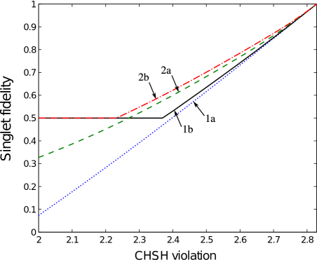
Figure 2: Minimal singlet fidelity as a function of CHSH violation. Curves 1(2) correspond to lowerbounds on the fidelity for generic(isotropic) boxes. Curves a(b) were obtained with the un-modified(improved) swap operator.

The new curves display a different behavior in two regions. When $CHSH\gtrsim 2.37$ (or $CHSH\gtrsim 2.23$ in the isotropic case), an appropriate choice of $\zeta_{A}$, $\zeta_{B}$, $W_{A}$, $W_{B}$ together with $\xi_{A}=\xi_{B}=\pi/2$ results in an improved bound on the fidelity compared to the standard SWAP procedure. For lower CHSH violations, however, the best choice of swap operator is obtained with $\xi_{A}=\xi_{B}=0$, resulting in a singlet fidelity of $1/2$. This value is thus obtained by comparing the ancilla rather than the state inside the box to the singlet (or equivalently by considering the local isometry that maps every local Hilbert space to the pure state $|0\rangle$). It thus corresponds to a trivial singlet fidelity, that can be certified up to local isometries regardless of the measured state. Clearly, any self-testing performed up to local isometries admits a trivial fidelity bound of this kind.

One can check that the curve 1a can be saturated by some two-qubit states and measurements when the standard swap (4, 8) and reference state $|\overline{\psi}\rangle$ are used. This bound is thus tight under this condition. Therefore, a modification of the SWAP procedure was necessary to improve this bound. It would be interesting to see if the improved bounds can be improved further or if they are close to optimal.

The fact that the bounds obtained in the isotropic and generic case differ in the first region suggests that the CHSH inequality is not optimal to bound the singlet fidelity of singlets subject to uniform noise. Upon examination of the dual of our SDP, we find that a better Bell expression to consider is of the form

$$I_{\alpha,\beta}=\alpha\langle A_{0}B_{0}\rangle+\langle A_{0}B_{1}\rangle+\langle A_{1}B_{0}\rangle-\beta\langle A_{1}B_{1}\rangle\,,$$ (36)

where $\alpha,\beta>0$ are parameters which depend on the quality of the statistics.

Note that an inequality of the same form, but with different values for the coefficients $\alpha$, $\beta$, was also shown to be relevant for randomness certification in presence of a Werner state olmo ; moreMore .

Comparison with previous bounds on the singlet fidelity from the CHSH violation

Previous to this work, most self-testing bounds were given in terms of the norm of the difference between the desired state $|\overline{\psi}\rangle_{A^{\prime}B^{\prime}}\otimes|\textrm{junk}\rangle_{AB}$ and the actual one after the isometry $|\psi\rangle_{A^{\prime}B^{\prime}AB}$, i.e. in the form

$$|||\psi\rangle-|\overline{\psi}\rangle\otimes|\textrm{junk}\rangle|| \leq t\,.$$ (37)

As a consequence,

$$t^{2} \geq 2-2s$$

where the scalar product $s=\langle\psi|\overline{\psi}\otimes\textrm{junk}\rangle$ can be taken real and positive since everything is defined up to a local unitary, so in particular it is possible to add a suitable global phase.

In this text we work with the singlet fidelity evaluated on the swapped state, i.e. $F=\langle\overline{\psi}|\rho_{\text{swap}}|\overline{\psi}\rangle$. In Appendix A, we show that both quantities are related through

$$s^{2}\geq 2F-1.$$ (38)

For a CHSH violation of $2\sqrt{2}-\epsilon$, curve $1b$ in Figure 2 gives a lower bound of approximately $F\gtrsim 1-1.1\epsilon$. We thus have that

$$|||\psi\rangle-|\overline{\psi}\rangle\otimes|\textrm{junk}\rangle||^{2} = 2(1-s)$$ (39)

$$\leq 2-2\sqrt{2F-1}$$

$$\lesssim 2.2\epsilon.$$

In the work of McKague et al. mckague , the values of $t$ are given explicitly by replacing $\epsilon_{1}$ and $\epsilon_{2}$ with the values given in Theorem 2 for CHSH and in Theorem 3 for Mayers-Yao, which gives:

$$|||\psi\rangle-|\overline{\psi}\rangle\otimes|\textrm{junk}\rangle||^{2} \lesssim 100\sqrt{\epsilon}$$ (40)

Note that this bound is not linear in $\epsilon$, and thus seems harder to compare with (39). However, one can see that this bound quickly becomes trivial. Indeed, already for $\epsilon\simeq 2.2\cdot 10^{-5}$, it yields a distance larger than $2-\sqrt{2}$, the distance between the singlet state and a product state.

In the work of Reichardt et al. reichardt , the bounds are not explicitly given, but can be reconstructed. The relevant result for comparison with our work is Lemma 4.2 in the long version reichardtlong , which refers to the single CHSH game (i.e. before the extension to parallel repetition that constitutes the main result of their work). With their notations:

$$\begin{split}|||&\bar{\psi}\rangle-|\psi^{*}\rangle\otimes|\psi^{\times}\rangle||^{2}\\ =&\,\sum_{c,i,j}||\psi_{cij}||^{2}\,|||\tilde{\psi}_{cij}\rangle-e^{i\phi_{cij}}|\psi^{*}\rangle||^{2}\\ &\stackrel{{\scriptstyle(*)}}{{\leq}}72284\,\sum_{c,i,j}||\psi_{cij}||^{2}\,\beta_{ij}\,\stackrel{{\scriptstyle(**)}}{{\lesssim}}10^{5}\,\epsilon\end{split}$$ (41)

where (*) comes from the end of proof of Proposition 4.5 and (**) from Eq. (4.4), using $72284*\sqrt{2}\approx 10^{5}$.

We see that our results are orders of magnitude better than the best previous results in the literature. Note also that no other results allow us to establish a non-trivial bound for the singlet fidelity in the best CHSH experiment realized so far Christensen13 . Curve $1b$ in Figure 2, on the other hand, allows one to certify a singlet fidelity greater than 99%.

IV.2 Singlet fidelity from Mayers-Yao

The work of Mayers and Yao, where the wording “self-testing” was first used, reported another criterion to self-test the maximally entangled state of two qubits. This time, $|\overline{\psi}\rangle=|\Phi^{+}\rangle$, the measurements are the same as (30) but there is a third setting on Alice’s side, ideally

$$\overline{A}_{2} = \frac{\sigma_{z}+\sigma_{x}}{\sqrt{2}}\,.$$ (42)

The ideal Mayers-Yao statistics, which self-tests $|\Phi^{+}\rangle$ with $F=1$, are given by

$$\begin{array}[]{lcl}\langle A_{0}B_{0}\rangle\,=\,\langle A_{1}B_{1}\rangle&=&1\\ \langle A_{0}B_{1}\rangle\,=\,\langle A_{1}B_{0}\rangle&=&0\\ \langle A_{2}B_{0}\rangle\,=\,\langle A_{2}B_{1}\rangle&=&\frac{1}{\sqrt{2}}\,.\end{array}$$ (43)

As for the CHSH example, we can just use the swap defined by (4) and (8) to obtain

$$F = \frac{1}{4}(1+\langle A_{0}B_{0}\rangle)\,+\,\frac{1}{16}\,\Big{(}\langle[A_{0},A_{1}][B_{0},B_{1}]\rangle$$ (44)

$$+\langle(A_{1}-A_{0}A_{1}A_{0})(B_{1}-B_{0}B_{1}B_{0})\rangle\Big{)}\,.$$

Notice that the setting $A_{2}$ does not appear in the construction of the swap, nor consequently in $F$; but it fulfills the crucial role of inducing constraints on higher moments of $A_{0},A_{1},B_{0},B_{1}$ in the SDP matrix.

For definiteness, we study the robustness of a mixture of ideal Mayers-Yao statistics (weight $v$) with white noise (weight $1-v$): that is, the statistics are given by the correlations (43) multiplied each by $v$. These are the correlations expected from using the prescribed measurements on a Werner state $\rho_{W}=v|\Phi^{+}\rangle\langle\Phi^{+}|+(1-v)\openone/4$ with visibility $v$.

Figure 3 shows the bound on the fidelity that we are able to certify from a direct application of our method for different values of $v$. We compare it to the analogous bound obtained from the CHSH violation achievable by the state and the actual fidelity of the Werner state. None of the lower bounds come close to the actual fidelity, thus suggesting that different measurements are necessary to optimally bound the singlet fidelity of Werner states in a device-independent manner.

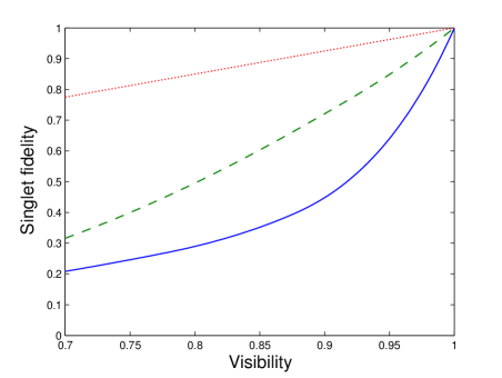
Figure 3: Lower bounds on the singlet fidelity of Werner states certified by the Mayers-Yao test (full line). Same bound as certified by the CHSH test is reported here from Figure 2 for comparison (dashed line). The dotted line is the actual fidelity of the Werner state itself.

IV.3 Complementary qubit measurements from CHSH

Suppose that, rather than verifying that $|\psi\rangle$ is close to $|\overline{\psi}\rangle$, we are interested in certifying to which degree Bob’s input $y$ is able to switch between the qubit dichotomic measurements $\sigma_{z},\sigma_{x}$. For that, we envision a virtual experiment in which we hand Bob a trusted qubit in a state $|\varphi\rangle$ unknown to him. We let Bob turn on an interaction between the trusted system and his box and only then we tell Bob which symbol $y=0,1$ to input. If the resulting statistics $P(b|y,|\phi\rangle)$ satisfy $P(b|0,|\varphi\rangle)=\langle\varphi|\frac{{\mathbb{I}}+(-1)^{b}\sigma_{z}}{2}|\varphi\rangle$, $P(b|1,|\varphi\rangle)=\langle\varphi|\frac{{\mathbb{I}}+(-1)^{b}\sigma_{x}}{2}|\varphi\rangle$, we conclude that Bob’s input indeed allows him to switch between the Pauli measurements $\sigma_{z},\sigma_{x}$.

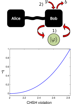
Figure 4: Estimation of Bob’s measurements. The protocol works in two steps: 1) We implement a full SWAP of Bob’s box and his trusted qubit, that we prepare in state $|\varphi\rangle$. 2) We implement measurement $B_{y}$ and study the resulting statistics.

Considering that Bob uses the swap operator specified in Eqs. (4, 8) as an interaction between the state $|\varphi\rangle$ and his box, he will observe outcome $b$, when later performing measurement $y$, with probability

$$P(b|y,|\varphi\rangle)=\mbox{tr}\left(M^{y}_{b}\cal{S}\rho_{AB}\otimes|\varphi\rangle_{B^{\prime}}\langle\varphi|\cal{S}^{\dagger}\right),$$ (45)

where $\cal{S}$ is given by Eq. (9).

To quantify the hypothesis $B_{0}=\sigma_{z},B_{1}=\sigma_{x}$, we define the figure of merit

$$\begin{split}\tau\equiv\,&\frac{1}{2}\left\{P(0|0,|0\rangle)+P(1|0,|1\rangle)+\right.\\ &\left.+P(0|1,|+\rangle)+P(1|1,|-\rangle)\right\}-1\end{split}$$ (46)

which compares statistics obtained when using different states for the ancillas. $\tau$ is a number ranging from -1 to +1, and $\tau=1$ is achievable only in the ideal case.

As before, $P(b|y,|\varphi\rangle)$ depends linearly on the moment vector $c$. For example:

$$P(0|0,|0\rangle)=\langle\psi|\left(\frac{{\mathbb{I}}+B_{0}}{2}\right)|\psi\rangle+$$

$$+\langle\psi|\left(\frac{{\mathbb{I}}-B_{0}}{2}\right)B_{1}\left(\frac{{\mathbb{I}}+B_{0}}{2}\right)B_{1}\left(\frac{{\mathbb{I}}-B_{0}}{2}\right)|\psi\rangle.$$ (47)

Consequently, $\tau=\tau({d})$, and so a lower bound on this quantity can be estimated with an SDP for measurements that are compatible with some Bell violation. The result of this computation for the case of measurements leading to some CHSH violation is shown in Figure 4, where $\tau$ indeed tends to 1 as the CHSH parameter gets closer to $2\sqrt{2}$.

IV.4 Fidelity of partially entangled two-qubit pure states

In Sections IV.1, IV.2, we have used quantum nonlocality to certify how close Alice and Bob’s state $|\psi\rangle$ is to a maximally entangled qubit pair. Here, we show how our method can be used to certify non-maximally entangled qubit pairs as well. This problem was first considered in yang , where an analytic estimate on the state fidelity was obtained. Here, using the SWAP concept, we derive a much better bound.

The scenario is similar to that used above to self-test the singlet state. The only difference is that we will use a tilted CHSH inequality of the form

$$\mathcal{B}_{\alpha}=\alpha\langle A_{0}\rangle+\langle A_{0}B_{0}\rangle+\langle A_{0}B_{1}\rangle+\langle A_{1}B_{0}\rangle-\langle A_{1}B_{1}\rangle,$$ (48)

where $0\leq\alpha\leq 2$. The maximum quantum violation of this inequality acintilted is given by $\sqrt{8+2\alpha^{2}}$ and the corresponding optimal qubit strategy is

$$\overline{A}_{0} =\sigma_{z},$$

$$\overline{A}_{1} =\sigma_{x},$$

$$\overline{B}_{0} =\cos\mu\;\sigma_{z}+\sin\mu\;\sigma_{x},$$

$$\overline{B}_{1} =\cos\mu\;\sigma_{z}-\sin\mu\;\sigma_{x},$$

$$|\overline{\psi}\rangle =\cos\theta|00\rangle+\sin\theta|11\rangle,$$ (49)

where $\sin 2\theta=\sqrt{(1-\alpha^{2}/4)/(1+\alpha^{2}/4)}$ and $\tan\mu=\sin 2\theta$. Thus, we can use the appropriate inequality with the corresponding value of $\alpha$ to device independently certify a reference state of the form $|\overline{\psi}\rangle=\cos\theta|00\rangle+\sin\theta|11\rangle$. The details on the construction of the swap operator are similar to those in Section IV.1, and can be found in Appendix B.

Figure 5 shows a plot of the minimal fidelity with $|\overline{\psi}\rangle$ for different values of $\alpha$ and different Bell inequality violations.

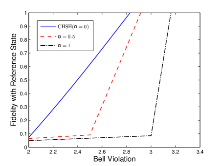
Figure 5: The solid line refers to the standard CHSH case, which obviously recovers the line in Figure 2. The dashed line refers to the case when $\alpha=0.5$ and the local bound is 2.5, explaining the discontinuity. The dotted-dashed line refers to the case when $\alpha=1$ and the local bound is 3.

The curves are approximately linear, between the local bound and maximum quantum bound. Since the local and quantum bound coincide at $\alpha=2$, the line gets steeper. This is expected, because, as $\alpha$ increases, the range of tolerable error gets smaller. However, it is interesting to note that the robustness is always close to linear for the three cases.

V New robust self-testing scenarios

V.1 Fidelity of a pure two-qutrit state from CGLMP

So far, our studied cases concern scenarios where Alice and Bob each have two inputs and two outputs, and they want to certify their state against an entangled pair of qubits. In this section, we illustrate how to extend these ideas to higher dimensional scenarios. It is unclear how one can generalize the methods sketched in mckague ; reichardt ; yang for such a purpose. However, using the SWAP method above, it is easy to do so.

The relevant Bell inequality for this case is the CGLMP inequality cglmp ; it requires two measurement settings on each side, with three measurement outcomes. The inequality reads:

$$\mathcal{B}_{\mathrm{CGLMP}}(p)=p(a<b|x=1,y=1)+$$

$$+p(a>b|x=0,y=1)+p(a\geq b|x=1,y=0)+$$

$$+p(a<b|x=0,y=0)\geq 1.$$ (50)

The maximum quantum violation is conjectured conject and verified numerically navascues to be $\mathcal{B}_{\mathrm{CGLMP}}(p)=(12-\sqrt{33})/9\approx 0.6950$. Moreover, it is believed that the maximal quantum violation can only be achieved with the (non-maximally entangled) state and measurement operators described in conject ; cglmp . Here we will prove this conjecture true.

First of all, let us re-express the state and measurement of conject ; cglmp in real form. This can be achieved by choosing the first measurements of Alice’s and Bob’s to be $\overline{E}_{m}^{0}=\overline{F}_{m}^{0}=|m\rangle\langle m|$ for $m=0,1,2$, the second ones $\overline{E}_{m}^{1}=\overline{F}_{m}^{1}=|\alpha_{m}\rangle\!\langle\alpha_{m}|$ with

$$|\alpha_{m}\rangle=\dfrac{1}{3}\left(2|m\rangle+2|m+1\rangle-|m+2\rangle\right),\\$$ (51)

and the state $|\overline{\psi}\rangle$ to be measured is as follows:

$$|\overline{\psi}\rangle =\dfrac{1}{3\sqrt{2+\gamma^{2}}}\left((\gamma+\sqrt{3})(|00\rangle+|11\rangle+|22\rangle)+\right.$$

$$\hskip 62.59596pt\gamma(|01\rangle+|12\rangle+|20\rangle)+$$

$$\left.\hskip 62.59596pt(\gamma-\sqrt{3})(|02\rangle+|10\rangle+|21\rangle)\right).$$ (52)

Here all additions performed inside the kets are modulo 3.

The above measurements and states shall then be our reference system. To certify the state, as usual, Alice and Bob will each attach a trusted qutrit to the entangled pair. The next step is to construct CNOT operators with which to build a partial swap, see Section III. The key point is how to build the translation operator $P$ from the measurement projectors defined in Eq. (52). There are many choices to do so; we chose the simplest combination:

$$P =\sum_{i=0}^{2}\overline{E}^{0}_{i}\left(-\frac{1}{2}\overline{E}^{1}_{i}-2\overline{E}^{1}_{i+1}+\overline{E}^{1}_{i+2}\right)$$ (53)

which indeed is a translation operator mapping $|0\rangle\rightarrow|1\rangle\rightarrow|2\rangle\rightarrow|0\rangle$. Here, addition of indices is modulo 3. Since Alice and Bob’s optimal operators are identical, the above formula also applies to Bob’s settings if we replace $E$’s by $F$’s.

The choice above in Eq. (53) is a valid unitary operator only for the optimal strategy $E_{a}^{0}=|a\rangle\langle a|$ and $E_{a}^{1}=|\alpha_{a}\rangle\langle\alpha_{a}|$. In a device independent scenario there is no guarantee that this choice still defines a valid unitary operator. We therefore introduce an extra auxiliary (non-hermitian) operator, $\hat{P}_{A}$, with the constraint that $\hat{P}_{A}^{\dagger}P(E^{x}_{a})\geq 0$. For Bob’s side, the swap operators are defined exactly the same way as above for Alice. Thus, we require also another auxiliary operator $\hat{P}_{B}$. We therefore use two localizing matrices $\Gamma(\hat{P}_{A}^{\dagger}P(E^{x}_{a}),{d})$, $\Gamma(\hat{P}_{B}^{\dagger}P(F^{x}_{a}),{d})$ to self-test the CGMLP inequality. As mentioned in Section III.2.2, all three semidefinite matrices can be taken real here, since, for any feasible point $\overline{{d}}$ of the corresponding complex SDP, the real vector $\mbox{Re}\{\overline{{d}}\}$ returns the same state fidelity, and the real matrices $\Gamma(\mbox{Re}\{\overline{{d}}\}),\bar{\Gamma}(\hat{P}_{A}^{\dagger}P(E^{x}_{a}),\mbox{Re}\{\overline{{d}}\}),\bar{\Gamma}(\hat{P}_{B}^{\dagger}P(F^{x}_{a}),\mbox{Re}\{\overline{{d}}\})$ are also positive semidefinite and satisfy the appropriate linear constraints.

Figure 6 shows a plot of the minimum fidelity with respect to the reference state $|\overline{\psi}\rangle$ as a function of the CGLMP violation.

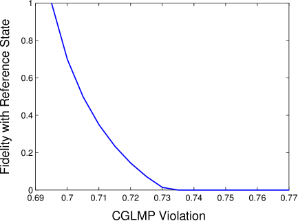
Figure 6: Minimum fidelity of the state swapped out the operators defined above. The blue line represents the minimum fidelity obtained from the SDP hierarchy. The hierarchy we used is the smallest hierarchy possible for the problem to be defined.

One can see that, as the violation tends to the quantum minimum ($\approx$ 0.6950), the fidelity of the general black box with respect to the reference state (non maximally entangled state) tends to 1. This shows that any quantum system violating the CGLMP inequality maximally is equivalent via local isometries to the non-maximally entangled state described in conject . This proves the conjecture that only non-maximally entangled states can violate CGLMP maximally.

V.2 Certification of entangled measurements

In Ref. rafael an entanglement-swapping based protocol to certify entangled measurements in a device-independent way is presented. In this protocol, four parties, A, B, C_A, C_B are allowed to conduct one out of two possible dichotomic measurements in their respective subsystems. By showing a maximal violation of the CHSH inequality between parties A, C_A and B, C_B, the state shared by Alice and Bob is certified to be separable. Then parties C_A, C_B are brought together and a collective measurement $C$ with four possible outcomes is conducted on the joint system C_A-C_B. As shown in rafael , if, conditioned on any of $C$’s outcome, Alice and Bob observe an absolute value for CHSH larger than $\sqrt{2}$, then measurement $C$ must be entangled.

Unfortunately, the previous protocol relies on the assumption that parties A, C_A or B, C_B violate CHSH maximally. This assumption is crucial to identify the degrees of freedom in parties C_A and C_B on which to test for the effect of measurement $C$. Indeed, the maximal violation of both CHSHs identifies one qubit on each of these systems on which the authors of rafael show that the action of measurement $C$ is entangled. Without this identification, the experimental statistics can always be modeled with a separable POVM between two parts C_A and C_B of the joint system C. Indeed, consider the situation where C_A and C_B, in addition to the degrees of freedom relevant for their CHSH measurement, share extra pairs of maximally entangled states. Then, at the time of conducting measurement $C$, C_A can use the maximally entangled states to teleport her internal state to C_B, who, in turn, conducts measurement $C$ on his side. The resulting POVM allows one to implement effectively measurement $C$ on C_A and C_B’s internal states, and is achievable via 1-way Local Operations and Classical Communication (and is, hence, separable). Therefore, we say that a measurement is entangled if one can identify local degrees of freedom on which its action is entangled.

In order to single out appropriate degrees of freedom where to test the action of measurement $C$ for non-maximal CHSH violations, we make use of the SWAP tool (see Figure 7). Namely, we present a trusted qubit system to each of C_A and C_B that we swap inside the two parties’ boxes with the help of the unitary swaps $\SS_{A}$ and $\SS_{B}$. These local unitaries define a qubit degree of freedom inside each party’s system. We then test whether the action of measurement $C$ on these particular degrees of freedom is entangled by analysing the state of two additional qubits (systems 1 and 2 in Figure 7) initially choosen to be maximally entangled with the two swapped qubits.

We choose to analyse the state of these two qubits conditioned on one of the possible outcomes of the joint measurement $C$ (as opposed to conditioning on four possible outcomes as in rafael ). It is thus sufficient to consider that $C$ can either produce the value $c=+1$ or $c=-1$, where $+1$ denotes ‘success’ of the measurement, i.e. projection onto one Bell state, and $-1$ denotes projection onto one of the three remaining Bell states. The state of interest is then $\rho_{12|c=1}$. Obviously, if $C$ can be described as a separable operator on the degrees of freedom considered, $\rho_{12|c=1}$ cannot be entangled at the end of the procedure. We can quantify the entanglement of the state $\rho_{12|c=1}$ via its negativity $\mathcal{N}$ computable , which, although non-linear in the components of $\rho_{12|c=1}$, can be estimated via SDP moroder .

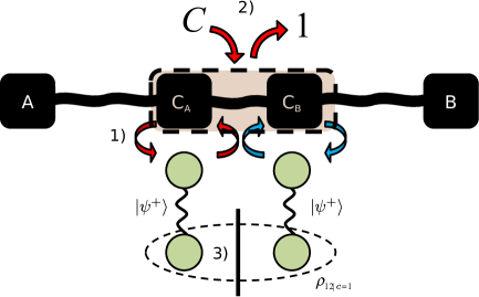
Figure 7: Certification of non-separability of the measurement $C$. The scheme works as follows: 1) We perform a (local) swap between the boxes C_A, C_B and two particles, each maximally entangled with particles 1, 2, respectively. 2) We perform measurement $C$ and post-select on result $c=1$. 3) We minimize the negativity of the state $\rho_{12|c=1}$.

This negativity can be bounded as a function of the following three inequalities:

$$\mathcal{B}_{1} =\langle A_{0}C_{0}^{A}\rangle+\langle A_{0}C_{1}^{A}\rangle+\langle A_{1}C_{0}^{A}\rangle-\langle A_{1}C_{1}^{A}\rangle\leq 2,$$

$$\mathcal{B}_{2} =\langle B_{0}C_{0}^{B}\rangle+\langle B_{0}C_{1}^{B}\rangle+\langle B_{1}C_{0}^{B}\rangle-\langle B_{1}C_{1}^{B}\rangle\leq 2,$$

$$\mathcal{B}_{3} =\langle(1+C)(A_{0}B_{0}+A_{0}B_{1}+A_{1}B_{0}-A_{1}B_{1})\rangle$$

$$\ \ \ -2\langle C\rangle\leq 2,$$ (54)

by solving the following SDP program:

$$f^{S}=\min\;\; \mbox{tr}(\sigma_{-})$$

s.t. $$\Gamma^{S}({d})\geq 0$$

$$\rho_{12|c=1}=g({d})$$ (55)

$$\rho_{12|c=1}^{T_{1}}=\sigma_{+}-\sigma_{-}$$

$$\sigma_{\pm}\geq 0$$

$$\sum_{i}f_{i}^{B_{j}}({d}_{i})=\mathcal{B}_{j}\ ,\ j=1,2,3\ ,$$

where $\rho_{12|c=1}$ is a function of the entries of the moment matrix $\Gamma^{S}({d})$ which we denote by $g({d})$. The optimization runs over the moments ${d}$ and the hermitian matrices $\sigma_{\pm}$. Above, we made use of the variational formula for the negativity of a bipartite state computable . Note that $T_{1}$ denotes the partial transpose with respect to the first subsystem (c.f. also moroder ), and $f_{i}^{B_{j}}$ are the coefficients of the Bell inequality $\mathcal{B}_{j}$.

Figure 8 shows the minimum value of $E\equiv P(c=1)\mathcal{N}\left(\rho_{12|c=1}\right)$ when the Bell violations are chosen to be the ones expected from perfect measurements on two Werner states $\rho=V|\psi^{-}\rangle\langle\psi^{-}|+(1-V)\openone/4$ with $\epsilon=2\sqrt{2}(1-V)$ up to first order in $\epsilon$, i.e. $\mathcal{B}_{1}=\mathcal{B}_{2}=2\sqrt{2}-\epsilon$, $\mathcal{B}_{3}=1+\sqrt{2}-\epsilon.$

The values in Figure 8 were obtained by using the SeDuMi sedumi package in Matlab. The three distinct curves correspond to different relaxations of the SDP problem with respective dimensions 144, 168, and 200 of the moment matrix $\Gamma^{S}(c)$. At the highest NPA level 3 (corresponding to a 200 dimensional moment matrix), we find that for $\epsilon<0.023$ the action of measurement $C$ on the degrees of freedom identified by the SWAPs cannot be described by a separable POVM. In the figure, we may also observe that as $\epsilon$ goes to zero measurement $C$ tends to act as a Bell state measurement providing (close to) $E=1/8$.

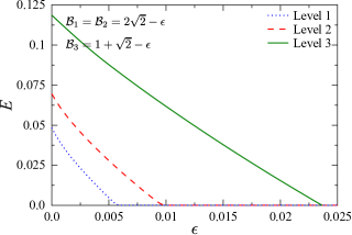
Figure 8: Certification of non-separability of measurement $C$. We minimize the quantity $E=P(c=1)\mathcal{N}\left(\rho_{12|c=1}\right)$ as a function of the value $\epsilon$, where $\mathcal{N}\left(\rho_{12|c=1}\right)$ denotes the negativity of the state $\rho_{12|c=1}$. The curves correspond to different levels of the NPA hierarchy navascues ; navascueslong . $E>0$ signals that Charlie’s measurement $C$ is entangled.

V.3 SWAP and maximally mixed states: work extraction and dimension estimates

The relation between work and information has been a matter of scientific debate since the dawn of statistical mechanics. In this regard, it has been shown in szilard ; oscar that the knowledge of the state of a quantum system, as measured by the smooth min and max entropies, can be used to generate work. Since the SWAP tool allows us to acquire knowledge about the state inside the box, it is hence not surprising that it can also lower bound its potential for work extraction.

In Figure 9 we use local swaps over two maximally mixed trusted qubits initially inside a Szilard engine in contact with a bath at temperature $T$. Since by definition the state of a maximally mixed qubit is completely unknown, such states can be considered as a free resource. After the interaction with the box, the state of the two qubits gets purified, and they can be rotated to one of the sides of the box with high probability, thus pulling a weight. Under the assumption that the energy operator of the system inside the box is fully degenerate, it can be proven that the amount of work extracted in this way is related to the difference between the maximum and minimum eigenvalues of $\rho_{\mbox{swap}}$, see Appendix C. This difference can be estimated via semidefinite programming. Figure 10 shows a plot of the CHSH violation vs the minimum amount of work extractable via this scheme. Notice that work extraction is possible as long as the system is non-local. Also, for the maximal CHSH violation, the amount of work extractable per $KT$ is $W/KT=2\ln(2)$, the work content of two pure qubits work_pure ; work_pure2 .

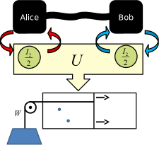
Figure 9: Non-locality and work. We let the boxes interact unitarily with two maximally mixed qubits, representing the position of two particles in a Szilard engine. The resulting pure state can then be rotated so that both particles end up on the left side of the engine with very high probability, hence producing storable work.

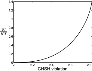
Figure 10: Extractable work per $KT$ as a function of the CHSH violation of an isotropic box.

In more complex non-locality scenarios, similar optimizations over the spectrum of the swapped state could also give clues about the dimensionality of the state inside Alice and Bob’s boxes. In noisy_op , it is proven that a state $\rho\in B({\cal H})$ can be transformed into a state $\sigma\in B({\cal H})$ by means of unitary transformations over $\rho$ and maximally mixed ancillas iff $\rho$ majorizes $\sigma$, i.e., if $\sum_{i=1}^{k}\lambda_{i}(\rho)\geq\sum_{i=1}^{k}\lambda_{i}(\sigma)$, for all $k$ (here $\lambda_{i}(M)$ denotes the $i^{th}$ greatest eigenvalue of the matrix $M$). Now, let $\rho_{\mbox{box}}\in B({\mathbb{C}}^{D})$ be the state inside the box(es), and consider the transformation $\rho=\rho_{\mbox{box}}\otimes({\mathbb{I}}_{d}/d)\to\sigma=({\mathbb{I}}/D)\otimes\rho_{\mbox{swap}}$ that results from applying a swap operator between the box and a trusted qudit in the maximally mixed state, followed by the replacement of the state inside the box by a maximally mixed qudit. From noisy_op it follows that $\lambda_{1}(\rho)/d\geq\lambda_{1}(\rho_{\mbox{swap}})/D$, and so $D$ satisfies

$$D\geq d\lambda_{1}(\rho_{\text{swap}}).$$ (56)

By minimizing $\lambda_{1}(\rho_{\text{swap}})$, we could hence (in principle) lower bound the dimensionality $D$ of the system inside the box.

VI Conclusion

To appreciate and ultimately certify a quantum experiment, a considerable amount of detailed information about the internal workings of the experimental setup is generally needed. For instance, in typical ion-trap experiments ion the state of the ions is considered to be (approximately) embedded in a two-dimensional Hilbert space, and the behavior of the ion when subject to sequential laser pulses is well known. Without this knowledge, it would be difficult to make sense of most ion-trap experiments. Remarkably, there exist situations where this kind of information is not required in order to take advantage of a (possibly complex) system.

In this paper we have introduced the SWAP tool to characterize quantum systems in arbitrary Bell-type scenarios. We showed that it provides much stronger bounds for known self-testing procedures, compared to previously-known techniques. We also showed that it provides robust self-testing in new contexts, such as the self-testing of qutrit states and of entangled measurements. Finally, we used the SWAP tool to relate nonlocal correlations to work extraction and quantum dimension, demonstrating that the tool can be used to study a wide variety of properties. All of these results are naturally noise tolerant and were obtained from the sole knowledge of accessible statistics.

The generality of the method exposed here raises new questions: How far can one go with the device-independent approach? Are Hilbert spaces necessary at all? Could the whole field of quantum information science be reformulated as a theory of black boxes?

Appendix A Proof of relation (38)

In order to relate both quantities, we express $|\psi\rangle$ in the Schmidt decomposition

$$|\psi\rangle=\sum_{i\geq 1}\sqrt{p_{i}}|\psi_{i}\rangle_{A^{\prime}B^{\prime}}|\phi_{i}\rangle_{AB}.$$ (57)

A singlet fidelity $F$ with respect to $A^{\prime}B^{\prime}$ hence implies:

$$\sum_{i\geq 1}p_{i}|\langle\overline{\psi}|\psi_{i}\rangle|^{2}=F.$$ (58)

Notice that the left hand side is upperbounded by $p_{1}$ (assuming that the Schmidt coefficients are ordered decreasingly, i.e., that $p_{1}$ is the maximum).

On the other hand, we have that

$$p_{1}|\langle\overline{\psi}|\psi_{1}\rangle|^{2}+1-p_{1}\geq\sum_{i}p_{i}|\langle\overline{\psi}|\psi_{i}\rangle|^{2}=F.$$ (59)

Combining the last inequality with $p_{1}\geq F$, we get that

$$p_{1}|\langle\overline{\psi}|\psi_{1}\rangle|^{2}\geq 2F-1.$$ (60)

Finally, note that

$$s^{2} =\max_{|junk\rangle}|\langle\psi|(|\overline{\psi}\rangle\otimes|junk\rangle)|^{2}$$ (61)

$$\geq p_{1}|\langle\psi_{1}|\overline{\psi}\rangle|^{2}\geq 2F-1,$$

where the inequality follows from taking $|\mbox{junk}\rangle=|\phi_{1}\rangle$.

Appendix B Non-Maximally Entangled State Certification with the tilted CHSH inequality

For convenience, we shall work in the local basis such that Bob’s optimal measurements are $\overline{B}_{0}=\sigma_{z}$ and $\overline{B}_{1}=\cos(2\mu)\sigma_{z}-\sin(2\mu)\sigma_{x}$. Note that $\bar{B}_{1}$ is no longer $\sigma_{x}$, as in the CHSH case, thus the swap operator defined in (4) no longer works for Bob. We will have to construct the analog of $\sigma_{x}$ by combining the operators $B_{0}$ and $B_{1}$. We thus introduce an auxiliary dichotomic operator $B_{2}$, with $B_{2}^{2}={\mathbb{I}}$, and impose relations between $B_{0},B_{1},B_{2}$ such that $B_{2}$ behaves as if it is $(\cos(2\mu)B_{0}-B_{1})/\sin(2\mu)$. Following Section III, the appropriate constraint is

$$B_{2}\dfrac{\cos(2\mu)B_{0}-B_{1}}{\sin(2\mu)}\geq 0.$$ (62)

This will force $B_{2}$ to share the same eigenvectors as $(\cos(2\mu)B_{0}-B_{1})/\sin(2\mu)$, and will identify both operators in the optimal case.

The swap operators in this case will then be $\SS_{B}=U^{\prime}_{B}V^{\prime}_{B}U_{B}^{\prime}$, with

$$U^{\prime}_{B}=\left(\mathbb{I}\otimes|0\rangle\langle 0|+B_{2}\otimes|1\rangle\langle 1|\right),$$

$$V_{B}^{\prime}=\left(\dfrac{\mathbb{I}+B_{0}}{2}\otimes\mathbb{I}+\dfrac{\mathbb{I}-B_{0}}{2}\otimes\sigma_{x}\right),$$ (63)

while $\SS_{A}$ is the same as in Eq. (4).

With the introduction of this extra auxiliary operator, our moment matrix is now enlarged with effectively two operators on Alice’s side $(A_{0},A_{1})$ and three operators on Bob’s side $(B_{0},B_{1},B_{2})$. The constraint (62) is enforced by imposing that the localizing matrix defined by

$$\begin{split}\Gamma&\left(B_{2}\dfrac{\cos(2\mu)B_{0}-B_{1}}{\sin(2\mu)}\right)_{ss^{\prime}}\\ &=\frac{\cos(2\mu)}{\sin(2\mu)}{d}_{s^{\dagger}B_{2}B_{0}s^{\prime}}-\frac{1}{\sin(2\mu)}{d}_{s^{\dagger}B_{2}B_{1}s^{\prime}}\end{split}$$ (64)

is positive semidefinite.

Appendix C Work extraction

Let $\rho_{AB}$, with spectral decomposition $\rho_{AB}=\sum_{k=1}^{4}\lambda_{k}|\psi_{k}\rangle\!\langle\psi_{k}|$, describe the state of two particles in a Szilard engine of length $L$ and area $A$, with $\lambda_{i}\geq\lambda_{i+1}$. Denoting by $L$ ($R$) the state corresponding to a particle being on the left (right) of the Szilard engine, we can always apply a unitary $U$ over the state $\rho_{AB}$ such that $U|\psi_{1}\rangle=|L,L\rangle$, $U|\psi_{2}\rangle=|R,L\rangle$, $U|\psi_{3}\rangle=|L,R\rangle$, $U|\psi_{4}\rangle=|R,R\rangle$. It follows that a population of $N$ particle pairs in a Szilard engine, initially in state $\rho_{AB}^{\otimes N}$, can be brought to a situation where $N_{L}=N(\lambda_{1}-\lambda_{4}+1)$ particles are on the left side of the engine, and $N_{R}=N(\lambda_{4}-\lambda_{1}+1)$ are on the right side. If we place a movable wall connected to a weight on the left side of the engine (in contact with a bath at temperature $T$), the pressure over the wall is equal to

$$P=\frac{N_{L}KT}{Az}-\frac{N_{R}KT}{A(L-z)},$$ (65)

where $z$ denotes the position of the piston. At constant temperature, the equilibrium position of the piston is $z_{\mbox{eq}}=\frac{N_{L}L}{N_{L}+N_{R}}$. The work extracted in the process of moving the piston from $z=L/2$ to $z_{\mbox{eq}}$ is

$$W=\int_{L/2}^{z_{\mbox{eq}}}PAdz=$$

$$=KT\left\{N_{L}\ln\left(\frac{2N_{L}}{N_{L}+N_{R}}\right)+N_{R}\ln\left(\frac{2N_{R}}{N_{L}+N_{R}}\right)\right\}=:$$

$$:=W(\lambda_{1}-\lambda_{4}).$$ (66)

Finally, the minimum value of $\lambda_{4}-\lambda_{1}$ can be extracted from $\rho_{\mbox{swap}}$ via the following SDP:

$$\begin{split}\min\ &\mu_{1}-\mu_{4}\\ \mbox{s.t.}\ &\rho_{\mbox{swap}}-\mu_{4}{\mathbb{I}}\geq 0,\\ &\mu_{1}{\mathbb{I}}-\rho_{\mbox{swap}}\geq 0.\end{split}$$

Since

$$\rho_{\mbox{swap}}-\mu_{4}{\mathbb{I}}\geq 0\Rightarrow\mbox{Re}\{\rho_{\mbox{swap}}\}-\mu_{4}{\mathbb{I}}\geq 0,$$

$$\mu_{1}{\mathbb{I}}-\rho_{\mbox{swap}}\geq 0\Rightarrow\mu_{1}{\mathbb{I}}-\mbox{Re}\{\rho_{\mbox{swap}}\}\geq 0,$$ (67)

it follows that the free variables in the corresponding SDP can be taken real, as in the previous examples.

References

- (1) A. Acín, N. Brunner, N. Gisin, S. Massar, S. Pironio and V. Scarani, Phys. Rev. Lett. 98, 230501 (2007).
- (2) S. Pironio, A. Acín, N. Brunner, N. Gisin, S. Massar, and V. Scarani, New J. Phys. 11, 045021 (2009).
- (3) Ll. Masanes, S. Pironio and A. Acín, Nat. Commun. 2, 238 (2011).
- (4) E. Hänggi and R. Renner, arXiv:1009.1833 (2010).
- (5) S. Pironio, Ll. Masanes, A. Leverrier and A. Acín, Phys. Rev. X 3, 031007 (2013).
- (6) R. Colbeck, A. Kent, J. Phys. A: Math. Theor. 44, 095305 (2011)
- (7) S. Pironio, A. Acín, S. Massar, A.B. de la Giroday, D.N. Matsukevich, P. Maunz, S. Olmschenk, D. Hayes, L. Luo, T.A. Manning and C. Monroe, Nature 464, 1021 (2010).
- (8) V. Scarani, Acta Physica Slovaca 62, 347 (2012).
- (9) N. Brunner, D. Cavalcanti, S. Pironio, V. Scarani and S. Wehner, Rev. Mod. Phys. 86, 419 (2014).
- (10) J.-D. Bancal, N. Gisin, Y.-C. Liang, S. Pironio, Phys. Rev. Lett. 106, 250404 (2011).
- (11) N. Brunner, S. Pironio, A. Acín, N. Gisin, A. A. Methot, V. Scarani, Phys. Rev. Lett. 100, 210503 (2008).
- (12) M. Tomamichel, E. Hänggi, J. Phys. A: Math. Theor. 46, 055301 (2013).
- (13) C.-E. Bardyn, T. C. H. Liew, S. Massar, M. McKague, V. Scarani, Phys. Rev. A 80, 062327 (2009).
- (14) T. Moroder, J.-D. Bancal, Y.-C. Liang, M. Hofmann and O. Gühne, Phys. Rev. Lett. 111, 030501 (2013)
- (15) B. S. Tsirelson, Hadronic Journal Supplement 8, 329 (1993).
- (16) S.J. Summers, R.F. Werner, Commun. Math. Phys. 110, 247 (1987) [refer to Theorem 2.3]
- (17) S. Popescu, D. Rohrlich, Phys. Lett. A 169, 411, (1992).
- (18) J. F. Clauser, M. A. Horne, A. Shimony, and R. A. Holt, Phys. Rev. Lett. 23, 880 (1969).
- (19) B.S. Cirel’son, Lett. Math. Phys. 4 93, (1980).
- (20) D. Mayers and A. Yao, Quant. Inf. Comput. 4, 273 (2004).
- (21) T. Franz, F. Furrer and R.F. Werner, Phys. Rev. Lett. 106, 250502 (2011).
- (22) C.-E. Bardyn, T.C.H. Liew, S. Massar, M. McKague, and V. Scarani, Phys. Rev. A 80, 062327 (2009).
- (23) M. McKague, T.H. Yang, and V. Scarani, J. Phys. A: Math. Theor. 45, 455304 (2012).
- (24) C.A. Miller and Y. Shi, arXiv:1207.1819 (2012).
- (25) B.W. Reichardt, F. Unger and U. Vazirani, Nature 496 (2013).
- (26) T.H. Yang and M. Navascués, Phys. Rev. A 87, 050102(R) (2013).
- (27) T.H. Yang, T. Vértesi, J-D. Bancal, V. Scarani, and M. Navascués, Phys. Rev. Lett. 113, 040401 (2014).
- (28) M. Navascués, S. Pironio and A. Acín, Phys. Rev. Lett. 98 010401 (2007).
- (29) M. Navascués, S. Pironio and A. Acín, New J. Phys. 10 073013 (2008).
- (30) S.P. Boyd and L. Vandenberghe, Convex Optimization. Cambridge University Press, 2004.
- (31) T. Ito, H. Kobayashi and K. Matsumoto, arXiv:0810.0693v1 (2008).
- (32) T. Fritz, T. Netzer and A. Thom, arXiv:1207.0975 (2012).
- (33) N. Ozawa, J. Math. Phys. 54, 032202 (2013).
- (34) K. F. Pál and T. Vértesi, Phys. Rev. A 82, 022116 (2010).
- (35) M. Navascués, T. Cooney, D. Pérez-García and I. Villanueva, Found. Phys. 42, 985-995 (2012).
- (36) M. Takesaki. Theory of Operator Algebras I, Springer (1979).
- (37) S. Pironio, M. Navascués and A. Acín, SIAM J. Optim. Volume 20, Issue 5, pp. 2157-2180 (2010).
- (38) Y. Zhang, S. Glancy and E. Knill, Phys. Rev. A 84, 062118 (2011).
- (39) O. Nieto-Silleras, S. Pironio and J. Silman, New J. Phys. 16, 013035 (2014).
- (40) J-D. Bancal, L. Sheridan and V. Scarani, New J. Phys. 16, 033011 (2014).
- (41) J-D. Bancal, V. Scarani, arXiv:1407.0856
- (42) B.W. Reichardt, F. Unger, U. Vazirani, arXiv:1209.0448
- (43) B. G. Christensen et al., Phys. Rev. Lett. 111, 130406 (2013).
- (44) A. Acín, S. Massar and S. Pironio, Phys. Rev. Lett. 108, 100402 (2012).
- (45) D. Collins, N. Gisin, N. Linden, S. Massar and S. Popescu, Phys. Rev. Lett. 88, 040404 (2002).
- (46) A. Acín, T. Durt, N. Gisin, and J. I. Latorre, Phys. Rev. A 65, 052325 (2002).
- (47) R. Rabelo, M. Ho, D. Cavalcanti, N. Brunner and V. Scarani, Phys. Rev. Lett. 107, 050502 (2011).
- (48) G. Vidal, R.F. Werner, Phys. Rev. A 65, 032314 (2002).
- (49) J.F. Sturm, Optimization Methods and Software 11, 625 (1999).
- (50) L. Szilard, Z. Phys. 53, 840-56 (1929).
- (51) O. C. O. Dahlsten, R. Renner, E. Rieper and V. Vedral, New J. Phys. 13, 053015 (2011).
- (52) C.H. Bennett, Int. Jour. Theor. Phys. 21, No 12, (1982).
- (53) R. P. Feynman, (Addison-Wesley, Boston, 1998).
- (54) M. Horodecki, P. Horodecki, and J. Oppenheim, Phys. Rev. A 67, 10 (2003).
- (55) D. Leibfried, R. Blatt, C. Monroe and D. Wineland, Rev. Mod. Phys., 75, 281 (2003).