The XMM-Newton EPIC X-ray Light Curve Analysis of WR 6

Abstract

We obtained four pointings of over 100 ks each of the well-studied Wolf-Rayet star WR 6 with the XMM-Newton satellite. With a first paper emphasizing the results of spectral analysis, this follow-up highlights the X-ray variability clearly detected in all four pointings. However, phased light curves fail to confirm obvious cyclic behavior on the well-established 3.766 d period widely found at longer wavelengths. The data are of such quality that we were able to conduct a search for “event clustering” in the arrival times of X-ray photons. However, we fail to detect any such clustering. One possibility is that X-rays are generated in a stationary shock structure. In this context we favor a co-rotating interaction region (CIR) and present a phenomenological model for X-rays from a CIR structure. We show that a CIR has the potential to account simultaneously for the X-ray variability and constraints provided by the spectral analysis. Ultimately, the viability of the CIR model will require both intermittent long-term X-ray monitoring of WR 6 and better physical models of CIR X-ray production at large radii in stellar winds.

1 Introduction

X-ray emission from massive stars continues to demonstrate its importance for understanding these objects (e.g., Güdel & Nazé 2009). In particular, X-ray generation can be associated with nonthermal processes, like particle acceleration, or with irreversible thermal processes, like shocked flows. The hypersonic laboratory afforded us by these winds could yield any of these emission types, depending on the nature of the winds and the phenomena they support. Thus the observed X-rays give us a unique window into the processes that ultimately energize the interstellar medium and mediate galactic evolution (e.g., Leitherer et al. 2010). Previously known mechanisms for generating X-rays from the winds of massive stars include collisions in binary systems (e.g., Usov 1992; Stevens, Blondin, & Pollock 1992; Canto, Raga, & Wilkin 1996; Walder & Folini 2000; Parkin & Pittard 2008; Gayley 2009), shock production in magnetically confined wind streams (Babel & Montmerle 1997; Townsend, Owocki, & ud-Doula 2007; Li et al. 2008; Oskinova et al. 2011; Petit et al. 2013; Ignace, Oskinova, & Massa 2013), and time-dependent shocks arising from inherent instabilities in line-driven winds (Lucy & White 1980; Lucy 1982; Owocki, Castor, & Rybicki 1988; Feldmeier, Puls, & Pauldrach 1997; Dessart & Owocki 2003). The latter two mechanisms arise in single stars, and came as a surprise when they were originally detected (Seward et al. 1979; Harnden et al. 1979). The shocks from the line-driven instability (LDI) are expected to be somewhat weaker, perhaps in the characteristic temperature range $kT\sim 0.1-1$ keV, than the strong shocks from magnetically confined winds. However, it should be noted that both of these mechanisms operate relatively close to the star, as line driving occurs where the wind is accelerating and magnetic channeling requires strong fields. In this paper, we will comment on X-ray generation that is inferred to originate well beyond the acceleration zone of the wind.

We note that in the roughly four decades since the discovery of X-rays from massive stars, the quality of the information has increased markedly. Modern X-ray observatories like the XMM-Newton and Chandra telescopes have larger collecting area and better spectral resolution than ever before (e.g., Jansen et al. 2001; Weisskopf et al. 2002). Stellar winds are an example of an area that have been significantly impacted by these observational advances in the X-ray band. The target discussed here is a member of the class of Wolf-Rayet (WR) stars, a relatively rare type of massive star. Although rare, the WR stars command significant attention by virtue of their extreme winds and evolved states.

A topic of particular interest has been the production of X-ray emissions in the winds of single massive stars, like our source WR 6 (also EZ CMa and HD 50896). Here we present the second paper reporting on 439 ks of XMM-Newton time. Whereas the first report by Oskinova et al. (2012; hereafter Paper I) emphasized information content provided by XMM-Newton spectroscopy of WR 6, here the focus is on understanding the star’s wind structure through an analysis of the X-ray variability that it displays.

Wolf-Rayet (WR) stars are generally accepted to be a phase of massive star evolution prior to termination as core-collapse supernova (Lamers et al. 1991; Langer 2012). Hydrogen is observed at much lower abundances than solar, or may even be altogether absent. The WR stars come in three principal subgroups: nitrogen-rich, carbon-rich, and oxygen-rich, all of which are helium-rich. Our target, WR 6, is a WN4 star, indicating that it is an early-type star of the nitrogen-rich category (Hamann, Koesterke, & Wessolowski 1995; Hamann, Gräfener, & Liermann 2006). The winds of WR stars are also expected to suffer from the LDI mechanism (Gayley & Owocki 1995) and should thus emit X-rays similar to their O-type progenitors. However, the WR winds tend to be more massive than for O stars. In general the two types of wind have similar wind terminal speeds, $v_{\infty}$, in the 1,000–3,000 km s^-1 range, but WR stars have wind mass-loss rates $\dot{M}$ that are greater by up to an order of magnitude relative to O stars of similar luminosity. As a result the winds are far more dense than O star winds (e.g., Abbott et al. 1986; Bieging, Abbott, & Churchwell 1989). The large wind densities and metallicity of WR winds make them quite opaque for the X-rays. The large wind opacity was invoked in Oskinova et al. (2003) to explain the apparent lack of X-ray emitting single WC-type stars.

Perhaps the key result of the first paper is the measurement of resolved X-ray line profile shapes and properties that are consistent with X-ray emission that emerges from the wind at large radius (of order $10^{2}-10^{3}R_{\ast}$ in the wind, depending on the wavelength of observation). One evidence for this is the nominal $f/i$ ratios observed in He-like triplet species (Gabriel & Jordan 1969; Blumenthal, Drake, & Tucker 1972). Here “f” refers to the forbidden component and “i” the intercombination one. The ratio of fluxes in these emission lines is a diagnostic of pumping from the upper level of the “i” line to the “f” line. In the absence of such pumping, the ratio has a value predicted by intrinsic branching ratios (e.g., Porquet et al. 2001), but the ratio can be reduced by either collisions or radiative excitation. The former is only important at high densities that are either not present in winds, or present only at depths from which X-rays may have a difficult time emerging, so is not considered here. Radiative pumping is of more potentially ubiquitous importance in the UV-bright circumstellar environment of massive stars, and then the $f/i$ ratio becomes a diagnostic of the dilution of the stellar continuum, namely where in the wind X-ray emissions are formed (Waldron & Cassinelli 2001; Cassinelli et al. 2001).

For WR 6 the $f/i$ ratios are close to their intrinsic and unpumped values, placing lower limits in the wind for the radius of the X-ray emission (see Paper I). In addition, the line profiles are asymmetric in conformance with expectations for X-ray production that is distributed throughout, and substantially photoabsorbed by, a dense and metal-rich WR wind (Ignace 2001). This stands in considerable contrast to O star winds, where line profile shapes are often more symmetric in appearance, and $f/i$ ratios tend to show anomalous values that are consistent with UV pumping and therefore proximity of the hot X-ray emitting plasma to the stellar photospheres (e.g., Waldron & Cassinelli 2007).

Although the high degree of photoabsorption from the dense WR wind implies that observable emission would need to come from a large radius, possibly even $10^{3}$ stellar radii, the challenge for these results is to explain how any X-ray generating process in a single star could operate efficiently so far from the region where line driving and potentially strong magnetic fields could be present. In addition, WR 6 has a well-known “clock” in that it shows polarimetric and spectroscopic variability on a period of 3.766 days (e.g., Firmani et al. 1980), yet no binary companion has been detected. Moreover, the X-rays seem too soft and of too low a luminosity to be associated with a compact companion (e.g., Morel, St-Louis, & Marchenko 1997). Based on the enhanced hardness of the emission in WR 6 compared to O stars, Skinner et al. (2002) have suggested that a low-mass non-degenerate companion might explain the X-rays. However, for a mass of $M_{\ast}\sim 30M_{\odot}$ and a radius $R_{\ast}\sim 1R_{\odot}$, a 3.766 d period corresponds to a semi-major axis of only $30R_{\ast}$, which is about an order of magnitude smaller than the radius where optical depth unity is achieved by wind photoabsorption at 1 keV. Perhaps some hard emission from a wind collision onto a companion could emerge owing to the fact that the photoabsorption opacity declines steeply with increasing photon energy, but certainly little or no soft emission would escape. Also, the spectroscopic variability does not show the strict phase coherence from cycle to cycle that might be expected from a binary companion, but is consistent with a rotating star with stochastically varying features.

Given that the evidence so far favors a single-star hypothesis for WR 6, this presents difficulties in accounting for the observed X-rays. Theorists have appealed to large-scale clumping and porosity in stellar winds as a geometrical effect to allow for easier escape of X-ray photons (Feldmeier, Oskinova, & Hamann 2003; Owocki & Cohen 2006; Oskinova, Hamann, & Feldmeier 2007; Sundqvist et al. 2012). The evidence for clumping in massive star winds is certainly voluminous (e.g., Hillier 1991; Moffat & Robert 1994; Hamann & Koesterke 1998), and clumping ameliorates the X-ray emission-line profile asymmetries that result from smooth, non-clumped wind considerations.

Clumping on the smaller scale of the photon mean-free path, sometimes termed “microclumping,” provides no real help in terms of X-ray photon escape, because it serves only to enhance emissivity at fixed mass-loss rate. Given that optically thin photoabsorption is linear in density, it scales the same as does the mass-loss rate itself, and is generally already included in mass-loss estimates.

This paper reports on the analysis and interpretation of X-ray variability detected from WR 6. Section 2 provides a brief review of the dataset, which has been discussed more thoroughly in Paper I. Section 3 presents an analysis of the variability data, incorporating not only the recent XMM-Newton pointings, but also all prior pointings from archival data. Section 4 presents a discussion of the results in terms of potential causes, and explores the possibility of accounting for the observed variability in terms of a co-rotating interaction region (CIR) model. Concluding remarks are given in Section 5.

2 Observations

The X-ray data on WR 6 were taken with the X-Ray Multi-Mirror Satellite XMM-Newton. Its telescopes illuminate three different instruments which always operate simultaneously: RGS is a Reflection Grating Spectrometer, achieving a spectral resolution of 0.07 Å; RGS is not sensitive for wavelengths shorter than 5 Å. The other focal instruments MOS and PN cover the shorter wavelengths; their spectral resolution is modest ($E/\Delta E\approx 20-50$).

The data were obtained at four epochs in 2010 (Oct. 11 and 13, Nov. 4 and 6; see Tab. 1). The total exposure time of 439 ks was split into four individual parts. Each exposure was approximately 30 hr in duration. The observations were not strongly affected by soft proton background flares. Our data reduction involved standard procedures of the XMM-Newton Science Analysis System v.10.0. Figure 1 displays the observed EPIC spectrum for the full exposure provided during the first of our four pointings. The three colors are for instruments PN, MOS1, and MOS2. Spectral analysis was the focus of Paper I. Here we explore the implications of observed variable X-ray emissions from WR 6.

In order to display, analyze, and discuss the X-ray variability of WR 6, we have evaluated spectrum-integrated count rates from the three EPIC instruments. Given the stability of the EPIC-PN instrument, a combined count rate $\dot{C}_{\rm T}$ was determined from a simultaneous fit to the count rates in the three instruments assuming

$$\dot{\cal C}_{\rm T}=\dot{\cal C}_{\rm PN}=\frac{M(\dot{\cal C}_{\rm PN})}{M(\dot{\cal C}_{\rm M1})}\,\dot{\cal C}_{\rm M1}=\frac{M(\dot{\cal C}_{\rm PN})}{M(\dot{\cal C}_{\rm M2})}\,\dot{\cal C}_{\rm M2}.$$ (1)

where $M(x)$ represents the median of a set of values in an observation. Minimization techniques were used on image frames for the three independent detectors to obtain the best estimate of the combined count rate. Background counts were modeled as well and treated independently among the instruments. The final count rate $\dot{C}_{\rm T}$ represents that value for the source that statistically produces the most consistent results for all three instruments. In this way signal-to-noise is maximized to produce the most sensitive possible study of variability in WR 6 from our dataset.

Table 1: XMM-Newton Observations of WR 6

Dataset ID	Date	Duration
		(ks)
0652250501	2010-10-11	111
0652250601	2010-10-13	105
0652250701	2010-11-04	111
0652250101	2010-11-06	112

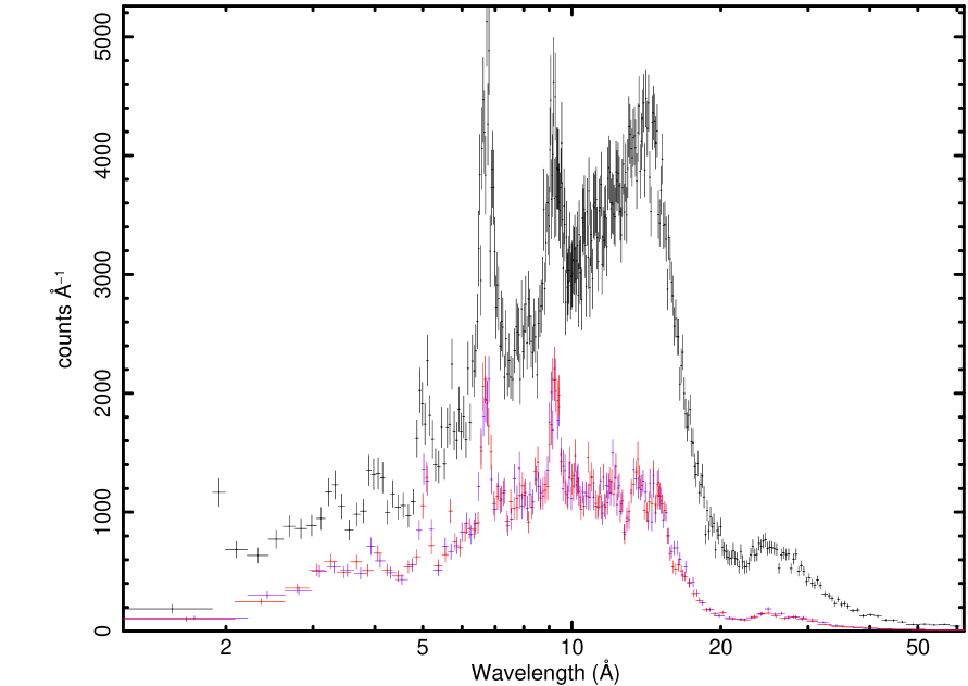
Figure 1: XMM-Newton PN (upper points in black), and MOS1 and MOS2 (lower points in red and blue) spectra of WR 6 obtained on 6 Nov 2010. The error bars correspond to 10$\sigma$. Note that the spectra are displayed as counts per Angstrom in a linear scale against wavelength in a logarithmic scale. Please refer to Paper I for a thorough discussion of spectral features.

3 Analysis

Our analysis of X-ray variability from WR 6 takes three basic forms. First, we consider event rate clustering, which seeks to determine whether the arrival of X-ray photons are clustered in time. Next we make a formal evaluation of the variability in WR 6 by considering the distribution of count rates from the star. Finally, we present light curves from the four pointings and phase these on the 3.766 d period of WR 6. We also consider how the source varies in different energy bands of the spectrum.

3.1 Event Rate Clustering

Such a long exposure has allowed us to search for clustering of X-ray detections in the event log of the detections. Clustering in the event log can provide a probe of spatially coherent shock structures within the wind that produce the detected X-ray flux. For example, consider a shock that develops instantaneously in the wind flow and cools: the time-dependent X-ray emission would take the form of a jump in counts followed by a period of decay characteristic of the cooling time. If the structure is substantially extended in a lateral sense, there could even be a modification to the temporal form of the signal (in both shape duration) owing to finite light travel time effects. This kind of “pulse” would lead to a clustering of detected events in the event log.

Natually, we would expect in a clumped wind flow that there are many of these shock events occuring throughout the flow. If X-ray photons were produced in an entirely random fashion, then we should expect a Poisson distribution for the detected events from a stochastic process. However, the physics of the shocks suggest that although the occurrence of shock events may be random, the signals that they produce are not.

Each of the four pontings to WR 6 provided an exposure of $\sim 10^{5}$ seconds and a listing of source detection events yielding roughly $\sim 60,000$ source counts per pointing for the PN detector. To test for clustering of events in photon arrival times, we conducted the following experiment. We chose a time interval $\Delta t$. With a given value of $\Delta t$, we step through an event list for one of the pointings. For an event occurring at time $t_{\rm i}$ for the $i^{\rm th}$ event, we count the number of additional neighboring events that fall in the interval $t_{\rm i}\pm\Delta t$. This is done for every event, and for a range of $\Delta t$ values.

Figure 2 displays the results of our experiment. The solid red line is based on the calculations for the data. It represents the number of events falling within $\pm\Delta t$ of a given event at time $t_{\rm i}$. These are normalized in such a way that the expectation from a Poisson distribution would be unity. The curve is plotted against the temporal “window,” $\Delta t$, in seconds. The purplish band is the $1\sigma$ error band indicating the dispersion about the expected value of unity for Poisson statistics. As can be seen, the data are quite consistent with pure Poisson noise: most of the curve lies within or very near the $1\sigma$ band.

As a test, we also experimented with simulated data. We imagine that X-rays are produced physically through shock events that we generically refer to as “flares”. The occurrence of a shock generates X-ray photons and events at the detector. We assume that a total number of $N$ equally bright flares are randomly distributed over the exposure in time. These flares are further assumed to cool exponentially, for which we adopt a characteristic cooling time of $10^{3}$ s. This rough cooling time is based on an estimate of the density and clumping in the wind. The dotted red curve in Figure 2 represents application of our event clustering diagnostic for a wind with $N=10^{4}$ flares. This curve lies well outside the $1\sigma$ band indicating that clustering would have been easily detected under these conditions if existing in the wind of WR 6. The implication seems to be that either there exist a very large number of “flare” events in the wind of WR 6 to suppress detection of event clustering, or the X-rays are produced in a stationary shock. The latter is something that we will explore further in Section 4.

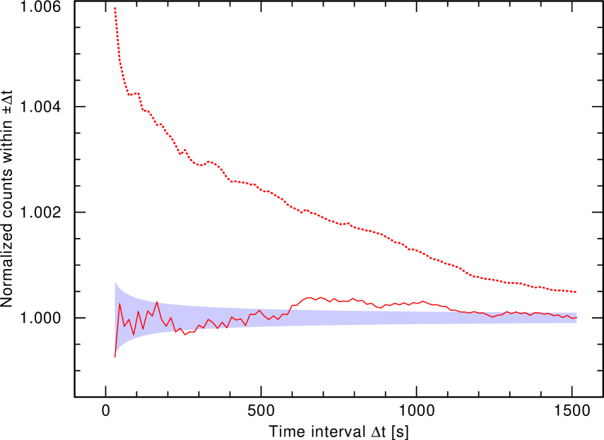
Figure 2: An event list with the $\sim 60,000$ source photons at the PN detector has been extracted from the $\sim 100,000$ s exposure for the fourth pointing and analyzed for clustering as described in the text. The data shown as the solid red line comply with completely random, un-clustered events, which would give unity in the normalized representation of the figure with one sigma of Poisson noise as indicated (purple shaded area). For comparison, simulated data assuming that $60,000$ photons were emitted in $10^{4}$ “flares”, randomly distributed over the exposure time, and each one decaying exponentially with a time scale of 1,000 s is displayed as the red dotted line. Despite the small number of only 6 photons per flare, our sensitive test would reveal a very significant degree of clustering.

3.2 Examination of Source Count Rates

Figure 3 displays a histogram of the total count rates obtained from the PN, MOS1, and MOS2 instruments. The count rates, in counts per second (cps), from all four pointings have been binned at 0.1 cps intervals to produce this figure of the frequency at which count rates appear in the data for WR 6. Note that the typical error in the count rate is about 0.007 cps.

The vertical green line in the figure signifies the mean count rate. Adopting notation that $\dot{{\cal C}}_{\rm i}$ is the total count rate for the $i$th sample, the mean value is given by an error-weighted sum:

$$\langle\dot{{\cal C}}\rangle=\frac{\sum_{i}^{N}\dot{{\cal C}}_{\rm i}/\sigma^{2}_{\rm i}}{\sum_{i}^{N}1/\sigma^{2}_{\rm i}},$$ (2)

where $\sigma_{\rm i}$ is the error in the $i$th count rate. The error in the average, $\sigma_{\rm av}$, is computed from

$$\sigma^{2}_{\rm av}=\frac{1}{N}\,\sum_{i}^{N}\sigma^{2}_{\rm i},$$ (3)

where $N$ is the number of count rate samples.

The magenta-hatched region in Figure 4 is a band of half-width $3\sigma_{\rm av}$. For a non-varying source, one would generally expect that over 99% of the count rate samples would fall within this band, for a normal distribution. As can be seen, the distribution of count rates is much broader than this hatched region; indeed, it appears to be bimodal, with a grouping of lower count rates at around 0.65 cps, and a less well-defined grouping at higher values of around 0.77 cps. It is clear that WR 6 displays substantial X-ray variability at the 10–20 % level over the duration of our dataset.

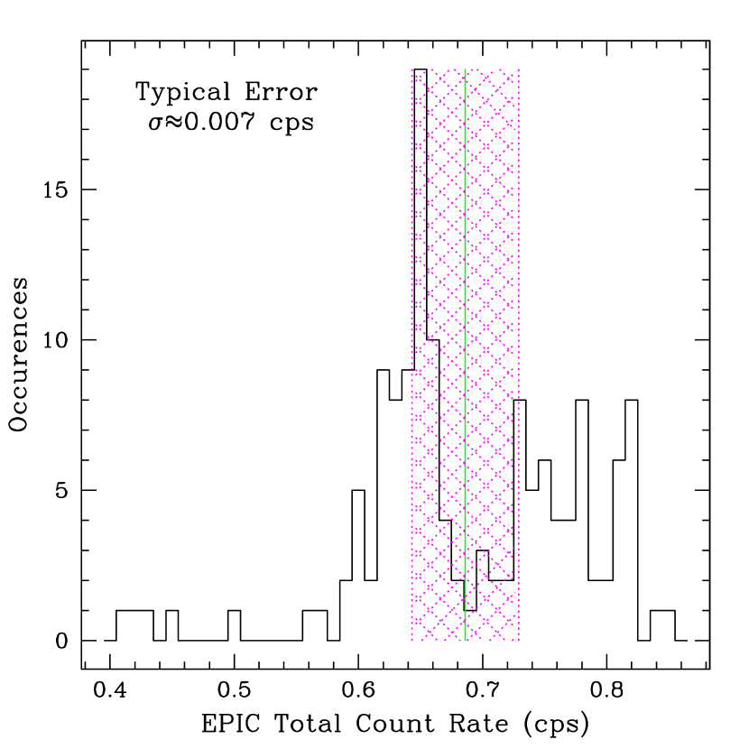
Figure 3: A histogram of the spectrum-integrated count rates (i.e., all four bands together) from the four new pointings using the EPIC detector. The vertical green line indicates the error-weighted average count rate. The magenta hatched region is the $3\sigma_{\rm av}$ band about this average, for which $\sigma_{\rm av}$ is the error in the mean count rate. The binning interval is 0.1 cps with 140 count rate samples.

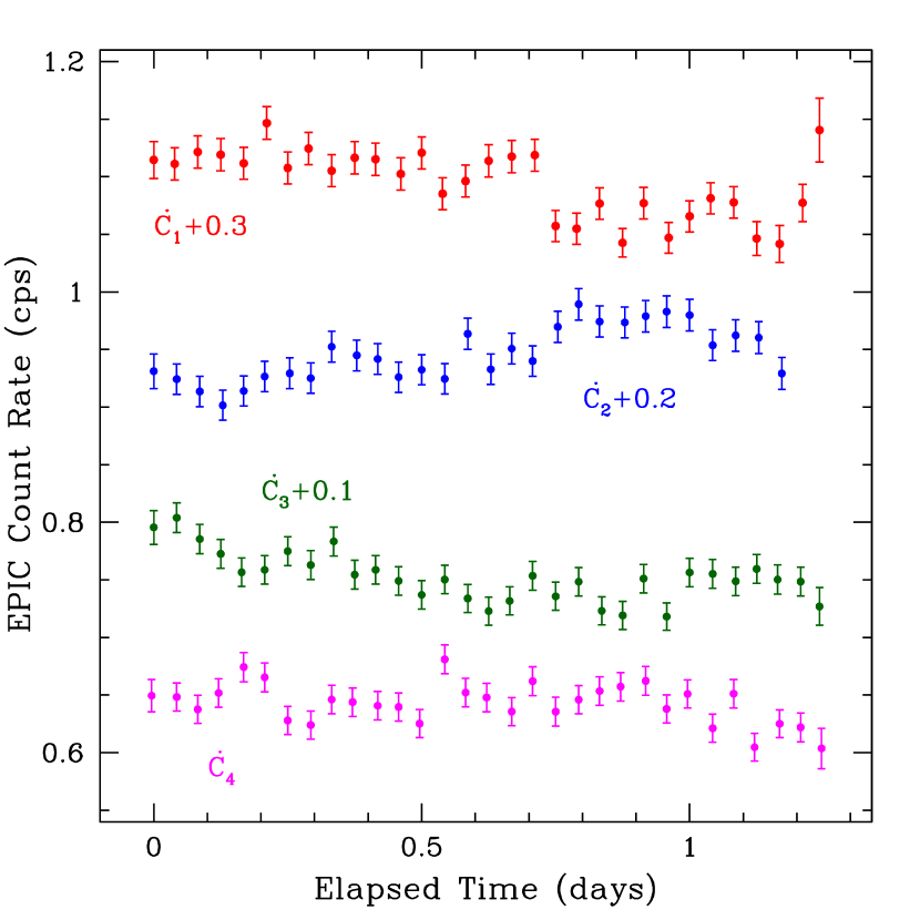
Figure 4: These are light curves for the four XMM-Newton pointings obtained for WR 6 plotted in counts per second with elapsed time. The total count rate is from integrating the entire EPIC spectra, including PN, MOS1, and MOS2, and averaging results for 3,600 second time bins. Elapsed time refers to days since the beginning each respective pointing. The separate pointings have been shifted vertically in count rate $\dot{\cal C}_{\rm T}$ as indicated. The four are displayed with the first at top, and the last at bottom. The count rates include $1\sigma$ errors.

3.3 X-ray Light Curves

Figure 4 shows light curves for our four separate pointings. These are total count rates $\dot{\cal C}_{\rm k}$ for $k=1$ to 4, signifying the sequence of pointings. The four light curves have been vertically shifted, as indicated, for clarity of viewing. The horizontal is elapsed time, in days, for each pointing separately. In other words each pointing is taken to begin at zero time. The binning of counts is over about 3,600 s for this figure. Variability is evident. Notable are trends that appear to persist throughout some of the pointings. For example, the second pointing suggests a steadily increasing count rate; by contrast, the third one indicates a declining one throughout the exposure.

Of particular interest for WR 6 is the well-known 3.766 d period that appears to govern variability in this star’s photometric, polarimetric, line emissions (Duijsens et al. 1996; St-Louis et al. 2009). The period is discerned in lines from the UV, optical, and IR. We have taken the total EPIC count rate data and phased the light curves on the 3.766 d period. The phased light curve is shown in Figure 5. Only data for our four pointings are shown in color: red for the first pointing, blue for the second, magenta for the third, and finally green for the fourth; these are the same colors as used in the preceding figure. Additionally, the black points refer to archival data. The phasing of data arbitrarily adopts the beginning of the pointing for the red dataset as zero phase. Note that the three measures shown as black circles near a phase of 0.2 are archival data in which “Thick” EPIC filters were used; Thick filter count rates tend to be about 20% lower than for the Medium filter.

Although the 3.766 d period is known to be stable over long timespans, meaning that this is a timescale that has been consistently observed over decades, there is no well-defined ephemeris for the variability. Although the timescale persists, the ephemeris appears to drift between epochs. Conseqently, it comes as no surprise that the archival data fail to line up with the more recent dataset. But perhaps it is surprising that the four pointings from the recent dataset also do not conform to a coherent phased light curve.

The XMM-Newton is not capable of obtaining a single continuous 439 ks light curve for a target source, and we did not request constrained observations. Even so, 439 ks is approximately four days of observing time, roughly equal to the known period. The four independent pointings have substantial overlap within that cycle. The second pointing (blue) was obtained about 1 day after the first pointing (red) was completed. The fourth pointing (green) was also obtained about 1 day following the completion of the third one (magenta). However, a time interval of about 3 weeks separate these two pairs, corresponding to about 6 cycles of the 3.766 d period. Although the two separate pairs show similar levels of variablity, the pairs are clearly shifted in terms of their relative average count rates. The error in a given sample count rate is about 0.01 cps, whereas the separate pairs of pointings have average count rates that are separated by roughly 0.1 cps. This separation is the cause for the bimodal appearance of total count rates seen in Figure 3.

To further elucidate the nature of this variability, we have formulated four energy bands to compare and contrast variability in the soft and hard portions of the X-ray spectrum. Table 2 introduces the definitions of these bands. The band count rates are shown in Figure 6 in an analogue to a color-magnitude diagram. The abscissa is the total EPIC count rate. The ordinate is a ratio of band count rates such as $\dot{{\cal C}}_{\rm j}/\dot{{\cal C}}_{2}$, for $j\neq 2$. Count rates from Band #2 were chosen as the normalization because its values were largest, and the errors smallest, plus it represents the majority of the counts from the observed spectrum. The red points are for $\dot{{\cal C}}_{1}/\dot{{\cal C}}_{2}$ for the softest emission relative to Band #2; green is for $\dot{{\cal C}}_{3}/\dot{{\cal C}}_{2}$ labeled as “Medium”, and blue is for $\dot{{\cal C}}_{4}/\dot{{\cal C}}_{2}$ for the hardest emission. Again, bimodality is evident in the appearance of a pair of vertically shifted groupings in total count rate within each relative color (see Fig. 3). Ignoring the especially low count-rate data, there appear to be some differences in the X-ray colors at the high ($\sim 0.8$ cps; hereafter “bright”) and low ($\sim 0.65$ cps; hereafter “dim”) count-rate pointings. These are summarized as follows:

• Relative to Band #2, all other Bands (1, 3, and 4) are less bright, hence $\dot{\cal C}_{\rm j}/\dot{\cal C}_{2}<1$.

• The Soft color (red points) is the strongest of the three shown, and the Hard color (blue points) is the weakest.

• The Medium color level is similar for both the bright and dim states. However, it appears that the Soft color level is noticably increased for the dim state as compared to the bright one. The same may be true for the Hard color, but if so, the change is less pronounced.

• There are a handful of “spurious” points at low count rates, below about 0.6 cps. We have ignored these in the discussion of trends above. However, it does seem that there have been instances when the X-ray brightness has at times dropped by nearly a factor of 2 relative to the observed bright state. At those times the Medium color appears to be greatest, and the Soft and Hard color levels are commensurate. In particular, it seems that the Soft color has dropped by a bit less than half, whereas the hard one has increased by a bit less than two. Such a spectral distribution could indicate a change in how the X-rays are generated, or might indicate a change in the amount of photoabsorptive absorption, perhaps the result of increased mass loss from the star.

Figure 5: The count rates of Figure 4 are here displayed as phased to the 3.766 d period of WR 6. An arbitrary zero point for the phasing was set to the beginning of the first of the four new pointings obtained by the authors. As in Figure 4, the first pointing is shown in red; the second in blue; the third in magenta; and the fourth in green. Black points are for archival data. Although variability is evident, there is no coherent X-ray light curve in terms of the 3.766 d period.

Table 2: Energy Bands

Band	Energy Interval
	(keV)
#1	0.3–0.6
#2	0.6–1.7
#3	1.7–2.7
#4	2.7–7.0

There is no doubt that WR 6 displays fairly significant variability of its X-ray emissions. In general, variability is a common property of WR stars. Among rigorously monitored WN stars, 40% show optical variability similar to WR 6 Chene et al. (2011). Our high-resolution X-ray spectra from Paper I indicate that the X-ray emitting plasma moves at about the same velocity as the cool wind, and the X-ray line blue-shifts do not change with time. Also, the X-ray emission-line spectrum is compatible with the WN star abundances. All of these facts are consistent with an interpretation of the X-rays as being endemic to a single-star wind. Nevertheless, whenever hard X-rays are generated at a large distance from a star, one must carefully eliminate the possibility of binarity before looking to more exotic explanations. But as mentioned previously, an orbital period of 3.766 days corresponds to an orbital semi-major axis for a low-mass companion of only $30R_{\ast}$, much less than the radius of optical depth unity in photoabsorption predicted from models (cf. Paper I) of about $10^{2}R_{\ast}$ at an energy of 1 keV. By contrast if a low-mass companion were situated out at a distance of $10^{2}R_{\ast}$, the orbital period $P_{\rm orb}$ would be at least 20 days, considerably longer than the 3.766 d “clock” inherent to WR 6.

Still, the challenge to explain X-ray emissions at large radii remains. Ignoring the clock in WR 6, if binarity is to be a plausible explanation for the observed X-rays, it seems that the companion would have to be in a somewhat large orbit of at least 100’s of $R_{\ast}$, with a period of a year. Our viewing perspective would likely need to be more pole-on than edge-on, to prevent drastic orbital modulation of the X-ray luminosity. It could be somewhat eccentric to produce longer term variations of the X-ray luminosity that are not too great in amplitude. Short-term variations (at the level of a day) in X-rays could then arise as an effect of instabilities in the structure of the colliding wind bow shock (e.g., Pittard & Stevens 1997), or as a result of a small number of very large wind clumps encountering the bow-shock region (e.g., Walder & Folini 2002).

A serious difficulty in ruling out either of those scenarios is that the wind flow time across a scale of $10^{2}-10^{3}R_{\ast}$ is half a day to days in duration, about the same as the UV periodicity. But the UV periodicity comes from much deeper in the wind where the flow time is much shorter, so the variabiilty there is more easily attributed to stellar rotation (St-Louis et al. 1995). Hence there remains the possibility that the concordance between the X-ray variability timescale and the UV variability timescale might simply reflect the coincidental matching of the flow time with the rotation period. However, if a more causally connected explanation is sought, binarity could not operate on the necessary timescale.

For definitively ruling out the binary explanation, there are some observational tests that would prove useful. First, WR 6 could be monitored in X-rays loosely at monthly intervals over a period of years to look for cyclic trends, rather than stochastic variations. Second, as it happens, the radio photosphere of WR 6’s wind is roughly similar in radial scale to the radius of optical depth unity for X-ray photoabsorption. The presence of a binary companion separated from WR 6 at a similar length scale should modify the effective shape of that photosphere, and so might cause modulation of the radio continuum light curve that would be correlated with X-ray variations. Both of these tests would require sparse, but dedicated, long-term monitoring of WR 6.

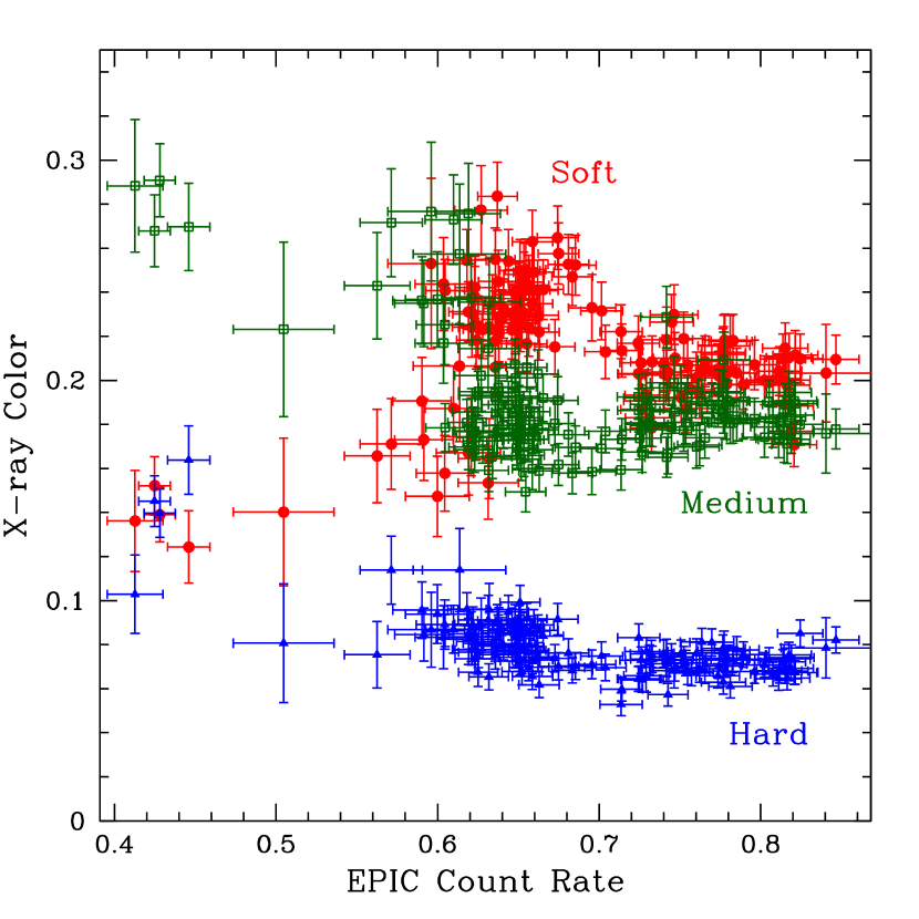
Figure 6: Similar to a color-magnitude plot, this figure shows three X-ray colors plotted against total EPIC count rate. The “colors” are ratios of the count rates from different bands 1, 3, and 4 to that of Band #2, which has the highest count rate among the respective bands. The red points are ratios of count rates $\dot{\cal C}_{1}/\dot{\cal C}_{2}$; green is for $\dot{\cal C}_{3}/\dot{\cal C}_{2}$, and blue is for $\dot{\cal C}_{4}/\dot{\cal C}_{2}$. The trends displayed in this figure are discussed in the text.

Here we explore the possibility of a non-binary explanation that unifies the 3.766 d period seen in other wavebands with the production of X-rays at large radius. Co-rotating interaction regions (CIRs) were proposed to explain a variety of observed phenomena in the solar wind and have long been invoked as a possible explanation for discrete absorption features observed in the UV lines of OB stars (e.g., Mullan 1984; Hamann et al. 2001), including WR 6 (St-Louis et al. 1995). A CIR arises from the interaction of wind flows that have different speeds: rotation of the star ultimately leads to a collision interaction between the different speed flows to produce a spiral pattern in the wind.

Recent new work has suggested the presence of a CIR in WR 6 and a few other WR stars showing similar variability in the optical (St-Louis et al. 2009; Chene et al. 2011; Chene & St-Louis 2011). We next consider a heuristic kinematic model of a CIR structure in the wind of WR 6 associated with the 3.766 d period in the form of stellar rotation.

4 Applying a CIR Model to the X-ray Variability

The motivation for the CIR is the idea that wind shocks degrade over time (Gayley 2013), and since the X-ray emission from WR 6 arises from large radii of $\sim 10^{2}-10^{3}R_{\ast}$, it is difficult to understand how the wind-shock paradigm could account for the presence of hot plasma. A CIR represents a globally ordered pattern that might conceivably persist to large radius, as seen in systems like the “dusty pinwheels” for WR binaries (e.g., Tuthill, Monnier, & Danchi 1999; Monnier, Tuthill, & Danchi 1999; Harries et al. 2004; Tuthill et al. 2008). In the application here, the CIR is associated with a single star and related to stellar rotation, not orbital revolution.

In what follows a description of a model for an equatorial CIR region is presented. A key assumption is that the observed X-ray emission forms at large radius in the flow owing to strong photoabsorption by the the dense WR wind. At large radii the wind mass density is approximately

$$\rho=\frac{\dot{M}}{4\pi\,r^{2}\,v_{\infty}}=\rho_{0}\,u^{2},$$ (4)

where the inverse radius $u=R_{\ast}/r$ is convenient to use in this analysis. The number density of electrons is then given by $n_{\rm e}=n_{0}\,u^{2}$, with $n_{0}\propto\rho_{0}\propto\dot{M}/v_{\infty}$.

Before introducing the CIR structure, it is first useful to review results for an otherwise smooth spherial wind as providing a background against which to interpret the influence of a CIR for variable X-ray emissions.

4.1 The Solution for a Smooth, Spherical Wind

Models for the X-ray generation produced throughout a wind have been discussed by numerous authors, and often parameterized in terms of a smooth, spherical wind flow with a volume filling factor of hot X-ray emitting plasma (e.g., Baum et al. 1992; Hillier et al. 1993; Owocki & Cohen 1999; Oskinova et al. 2001). Although the clumped nature of massive star winds has long been recognized, considerations of the smooth wind case has value in its simplicity and continues to provide broad insight into the main features of how a distribution of X-ray sources in a wind combine with wind photoabsorption effects to create an emergent X-ray spectrum. We consider a smooth wind model before turning to the more complex CIR case.

Imagine a spherically symmetric and laminar wind flow. Since the X-rays emerge only from large radius, we restrict ourselves to the use of equation (4) for an inverse square density law. One of the key factors governing the emergent X-ray spectrum is the wind photoabsorption. The optical depth $\tau$ of photoabsorption along a sightline through the spherical wind is given by

$$\tau=\int_{z}^{\infty}\,\kappa(E)\,\rho\,dz$$ (5)

where $z$ is the coordinate along the sightline of the observer (located at $+\infty$), and $\kappa(E)$ is the energy-dependent opacity for photoabsorption. The optical depth of photoabsorption has an analytic solution when $\rho\propto u^{2}$, as given by (e.g., Ignace 2001):

$$\tau(r,\theta,E) = \kappa(E)\,\rho_{0}\,R_{\ast}\times u\,\frac{\theta}{\sin\theta},$$ (6)

$$\equiv \tau_{0}(E)\,u\,\frac{\theta}{\sin\theta},$$ (7)

where $\theta$ is the polar angle from the observer’s axis, and $\tau_{0}(E)$ is a parameterization for the energy dependence of the optical depth.

The luminosity of presumably optically thin X-ray emission formally derives from a volume integral:

$$L(E)=\int dV\,\int dT\,{df\over dT}\,n^{2}(r)\,G(E,T)\,e^{-\tau(r,\theta,E)},$$ (8)

where $df/dT$ is the distribution of volume filling factor over $T$, and $G(E,T)$ is the appropriate kernel for collisional ionization equilibrium (neglecting density dependence) for distributing the X-ray emission over photon energy $E$. Making for simplicity the approximation that $df/dT$ does not depend on $r$, we can separate the $r$-independent terms into a single “emissivity profile” given by

$$\Psi(E)={1\over f_{V}}\,\int dT\,{df\over dT}\,G(E,T),$$ (9)

where $f_{V}=\int dT\,df/dT$ is the volume filling factor of hot gas, assumed constant. This separation yields

$$L(E)=\Psi(E)\int dV\,n^{2}(r)\,e^{-\tau(r,\theta,E)},$$ (10)

where the form of $\Psi(E)$ can then be chosen separately to mimic the actual spectrum. The interest here is on how the escape physics affects the total luminosity; the as-yet unspecified processes that shape the intrinsic emissivity profile $\Psi(E)$ can be addressed in future studies.

Substituting the previous relationships into the integrand, and evaluating both the azimuthal and radial integrations, the spectral energy distribution in the luminous output becomes

$$L(E) = 2\pi\,R_{\ast}^{3}\,f_{V}\,\frac{\Psi(E)}{\tau_{0}(E)}\times$$ (11)

$$\int_{0}^{\pi}\left[1-e^{-\tau_{0}\,\theta/\sin\theta}\right]\frac{\sin^{2}\theta}{\theta}d\theta.$$

In the limit that $\tau_{0}(E)\gg 1$, the second term in the brackets of the integrand vanishes, and the integral yields a constant value of 1.2188. In this case the luminous spectrum is

$$L(E)\propto\frac{\Psi(E)}{\tau_{0}(E)}.$$ (12)

Note that in this approach, and with $f_{V}$ a constant, the emergent spectral energy distribution (SED) is given strictly by the ratio of the energy-dependent profile function to the energy-dependent photoabsorptive opacity.

4.2 A CIR X-ray Source Model

To produce a reabsorbing environment that can show rotational modulation, we next introduce a simple CIR model in the form of a spiral pattern in the flow, following Ignace, Hubrig, & Schöller (2009) and Ignace, Bessey, & Price (2009). For a fixed radius, the CIR is taken to have a circular cross-section. The opening angle of this cross-section is denoted as $\gamma$. The equation of motion for the center of the spiral, in the limit that $r\gg R_{\ast}$, is given by

$$\varphi_{\rm c}(r)=\varphi_{0}+\omega\,t-\frac{r\,\omega}{v_{\infty}},$$ (13)

where $\omega=2\pi/P_{\rm rot}$, with $P_{\rm rot}$ the stellar rotation period, and $\varphi_{\rm c}$ the azimuth of the center as a function of radius. A characteristic length scale of this prescription is the “winding radius” given by

$$r_{\rm w}=v_{\infty}\,P_{\rm rot},$$ (14)

which represents the length traveled by the wind in one rotation period. Consequently, it is related to the asymptotic pitch angle of the spiral.

We assume that the CIR is the only source of X-ray emission at large radius in the wind. We are unaware of any calculations that would provide guidance as to the density and temperature distribution in such a structure at such distances. For simplicity, and in order to determine the potential plausibility of such a model, we will assume that the density of the hot plasma scales with the wind density (i.e., $r^{-2}$). We further adopt a hot-plasma emissivity profile $\Psi$ with the form of a power law in energy and a low-energy cut-off. The dominant form of cooling for hot plasma at the temperatures of interest is by lines. However, there are a great many weak lines in the spectrum, punctuated by several strong ones. For a low-resolution SED, sufficient for our exploratory model, the emission lines blend to form a pseudo-continuum. The adopted power-law form is roughly consistent with a multi-temperature plasma (e.g., Owocki & Cohen 2001); implicit is that the range of temperatures and the relative amount of emission measure per temperature interval are constants throughout the CIR.

So, the monochromatic luminosity is taken to be of the form:

$$L(E)=\Psi(E)\,\int\,n^{2}(r)\,e^{-\tau(r,\theta,E)}\,dV.$$ (15)

For the profile function, we adopt the following:

$$\Psi(E)=\Psi_{0}\,E^{-q_{2}}\,\left\{1-\exp\left[\left(E/E_{0}\right)^{q_{1}}\right]\right\},$$ (16)

where the observed X-ray spectrum (see Fig. 1) guides the selection of the constants $q_{1}$, $q_{2}$, and $E_{0}$. In our treatment only the CIR emits X-rays at the large radii of interests. X-rays that emit in the direction of the observer are still attenuated by the wind. To evaluate this absorption, we adopt a smooth wind for these purposes, for which the optical depth will be given by

$$\tau=\tau_{0}(E)\,\frac{R_{\ast}}{r}\,\frac{\theta_{\rm c}}{\sin\theta_{\rm c}},$$ (17)

where

$$\tau_{0}(E)=\kappa(E)\,\rho_{0}\,R_{\ast},$$ (18)

with

$$\rho_{0}=\frac{\dot{M}}{4\pi\,R_{\ast}^{2}\,v_{\infty}},$$ (19)

and

$$\kappa(E)=\kappa_{0}\,\left(E/1~{}{\rm keV}\right)^{-Q},$$ (20)

with $Q$ a constant. In our models the constants $\kappa_{0}$ and $\Psi_{0}$ are set to unity as we mainly seek to reproduce the overall shape of the observed X-ray spectrum. The remaining parameters are chosen to accomplish this end, with values of $E_{0}=0.6$ keV, $q_{1}=2.8$, $q_{2}=3.8$, and $Q=2.6$.

We assume that the CIR has a relatively small opening angle, so that the optical depth to the center of the structure at radius $r$ represents the column of absorbing material to the CIR’s entire cross-section at that radius. Then the resultant energy-dependent luminosity reduces to

$$L(E)=L_{0}(E)\,\int_{0}^{1}\,\tau_{0}(E)\,e^{-\tau_{0}(E)\,u\,\theta_{\rm c}/\sin\theta_{\rm c}}\,du,$$ (21)

where again $u=R_{\ast}/r$, and

$$L_{0}(E)=\pi\,\gamma^{2}\,n_{0}^{2}\,R_{\ast}^{3}\,\frac{\Psi(E)}{\tau_{0}(E)}.$$ (22)

The resultant X-ray spectrum separates into a pair of factors, one of which mimics the result of the smooth, spherical wind in the form of $L_{0}(E)$. The other factor is the implicit energy-dependent, and time-dependent, integration owing to the CIR structure.

The integral expression in equation (21) does not have a general analytic solution given that $\theta_{\rm c}=\theta_{\rm c}(u)$. However, there is a special case where a solution can be derived and which provides some insight for application to the observations of WR 6, even though it is not strictly appropriate. Consider the case of a long, straight CIR, which is the limit of $v_{\rm rot}\ll v_{\infty}$. Taking into account the photoabsorption of X-rays by the wind, “long” implies that $r_{1}\lesssim r_{\rm w}$ such that the CIR is effectively a cone over the relevant region of emission. In this limit the solution for the SED becomes

$$L(E)\propto\frac{\Psi(E)}{\tau_{0}(E)}\times\frac{\sin\theta_{\rm c}(t)}{\theta_{\rm c}(t)},$$ (23)

where from spherical trigonometric considerations

$$\cos\theta_{\rm c}=\sin i\,\cos\varphi_{\rm c}(t)=\sin i\,\cos(\Omega\,t).$$ (24)

In this limiting case, the viewing inclination sets the maximum amplitude of variation. But what is clearly evident is the cyclic nature of the variation. Allowing for the spiral nature of the CIR does not change the fact that the model produces cyclic variations at fixed $E$. However, relaxing the straight-arm cone to a spiral pattern does introduce phase shifts in the cyclic variability from one energy to the next.

A phase lag can be understood qualitatively by thinking in terms of how the spiral CIR intersects a sphere of the energy-dependent radius of unit optical in photoabsorption, $r_{1}(E)$. That intersection occurs at different azimuths for different energies because of the fact that $r_{1}$ is larger at softer energies and smaller at harder ones. Indeed, the azimuthal location of the CIR’s center at radius $r_{1}$ is given by $\varphi_{1}=\varphi_{\rm c}(t,r_{1})=\varphi_{\rm c}(t,E)$. Even so, X-ray bandpass count rates or fluxes will still be cyclic on the period of the stellar rotation. Additionally, because of the energy-dependent phase lags, the overall effect will be to reduce the amplitude of variation in a bandpass as compared to the monochromatic variability. Obtaining cycle-to-cycle variations requires a new ingredient to the model.

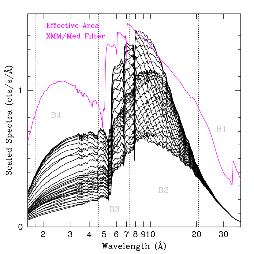
Figure 7: Linear-log overplot of synthetic XMM-EPIC spectra (PN+MOS1+MOS2) for the medium filter (area response in magenta) illustrating the variable SED arising from the CIR model. Vertical dotted lines in gray signify the bands B1–B4 used in this paper.

Figure 8: An example light curve for the total X-ray count rate $\dot{\cal C}_{\rm T}$ from our “wavy” CIR model. The count rate is normalized to have a peak value of unity; here the count rate is displayed as a percentage of the peak value. The abscissa is for cycles in terms of the 3.766 d period of WR 6. The model parameters in this exampe are for Model 17 from Tab. 3.

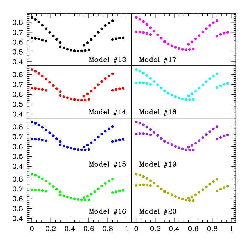
Figure 9: Example phased light curve with the modulated CIR model. These segments correspond to the observed phases of our four pointings. The parameters for these light curves are for models 13 to 20 from Table 3. All of the model light curves were scaled to have peak values similar to the observed count rates.

4.2.1 The Wavy CIR

The discussion of the preceding section for a steady-state CIR yielded a variable X-ray signal because of the wind photoabsorption in relation to the rotating and non-axisymmetric structure of the CIR. A CIR is a hydrodynamic phenomenon. It may be possible that its structure is influenced by hydrodynamic instabilities. CIR structures from the solar wind are fairly well-studied (e.g., Rouillard et al. 2008), and it is known that CIRs can merge at large distances in the solar wind, at around 10–20 AU (Burlaga, Schwenn, & Rosenbauer 1983; Burlaga, Ness, & Belcher 1997). Moreover, the large-scale solar magnetic field is dipolar but tilted somewhat to the rotation axis. This magnetic field can interact with a CIR leading to a “deflection” of the structure, meaning for example that spiral path of the CIR no longer resides in a single plane (Gosling & Pizzo 1999).

Merging and deflection of solar CIRs are complex effects, and it is difficult to speculate how such behavior in the solar wind might carry over to the highly unstable massive-star winds. Nonetheless, the case of the Sun informs us that there are processes that can modify CIR structures on time scales that are unrelated to the rotation of the star. Instabilities associated with line-driven wind theory or effects like those seen with solar CIRs can plausibly lead to variable structure in the CIR itself with consequent cycle-to-cycle (or epoch-to-epoch) variations in the X-ray emissions.

In an attempt to understand the X-ray variations of WR 6, we introduce a simple modification to the CIR structure. Given that one would not expect the rotation of the star to vary, there are two main options for our model: either the opening angle of the CIR or the wind terminal speed changes in time. The wind terminal speed would govern the pitch angle of the spiral as a function of time and location; the opening angle $\gamma$ would govern the solid angle of the CIR as a function of time and location. For purposes of illustration, we choose to allow for a variable opening angle of the CIR, which we refer to as the “wavy” CIR.

To accomplish this, we imagine a sinusoid wave propagating along the length of the CIR. We model the opening angle with

$$\gamma=\gamma_{0}\,\left[1+\delta\,\sin(Kr-\Omega t)\right],$$ (25)

indicating that the opening angle varies from $(1-\delta)\gamma_{0}$ to $(1+\delta)\gamma_{0}$. The wave parameters $K$ and $\Omega$ are related to the characteristic length and the period of the wave as $l_{\rm wav}=2\pi/K$ and $P_{\rm wav}=2\pi/\Omega$. The wave travels along the CIR at speed $v_{\rm CIR}=\Omega/K$. The combination of the wind photoabsorption with a non-axisymmetric spiral pattern and an additional time-varying CIR structure that is uncorrelated with the stellar rotation yields a generally cyclical X-ray light curve with an overlying cycle-to-cycle modulation.

In an exploration of model results, we have calculated a number of example models as shown in Figures 7–11. Parameters used for these models are listed in Table 3. Note that in this table, the wave parameters $\Omega$ and $K$ are given in terms of the stellar rotation period (in this case $P_{\rm rot}=3.766$ d) and the stellar radius. For example, all of the models use $\Omega=0.1/P_{\rm rot}$, meaning that the period of the propagating wave for the CIR is $P_{\rm wav}=2\pi/\Omega=20\pi\,P_{\rm rot}$.

We have not attempted to reproduce exactly the observed variations shown in Figure 5. Although the spiral pattern is physically motivated, the forms for the wavy CIR and the X-ray emission distributions are merely convenient prescriptions. Consequently, it is premature to attempt any quantitative fits to the data, and instead our focus is on the qualitative aspects of a CIR that might account for the observed variability.

Figure 7 shows the variable spectrum, in counts/s/Å, as a function of time. The black curves are model spectra at different times as the star rotates. Indicated in gray are the four energy bands used in our analysis. Also shown in magenta is the total XMM-Newton effective area, using a medium filter, as taken from the PIMMS software (Mukai 1993). The variations are relative to a reference spectrum of unit area.

An example of the long-term variability that can arise from a “wavy CIR” is displayed in Figure 8. The model parameters correspond to 17 of Table 3. The time axis is in terms of the number of cycles of the 3.776 day period for WR 6. With $\Omega=0.1$, the period of the CIR wave is $P_{\rm wav}/P_{\rm rot}\approx 63$ rotational cycles. The variable X-ray count rate is displayed as a percentage of the peak value obtained. The rapid variations are of course the 3.776 d period. The long term modulation reflects the time- and location-dependent opening angle of the CIR.

Figure 9 illustrates how the wavy CIR leads to disjoint phased light curves. Each panel is a model light curve, with model number indicated, phased on the 3.766 d period. The vertical is counts per second scaled to similar values as those observed. The segments correspond to the relative time durations and intervals for our four pointings. If $K$ and $\Omega$ were zero, the light curves would all be continuous; addition of a “wave” to the CIR structure leads to epoch-dependent variations in the total count rates.

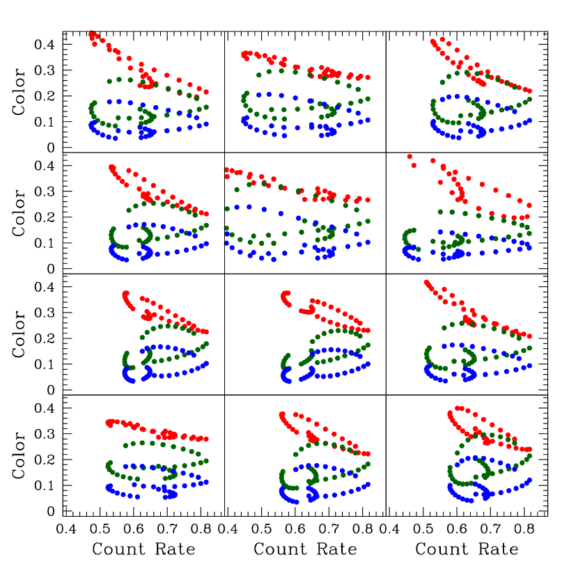
Figure 10: Models 1 to 12 as parameter study plotted as X-ray color versus count rate to mimic Fig. 6. The color scheme is the same as for Fig. 6, with red for Soft, green for Medium, and blue for Hard. The same relative phases are shown here as for the observations, but with a lower density of points. Model parameters are given in Tab. 3. From top to bottom, the panels are for models 1–4 at left, 5–8 in the middle, and 9–12 at right.

Figure 11: Models 13 to 20 with variations geared to match more closely those observed in WR 6. See Tab. 3 for the parameters. In particular the ratio $v_{\rm rot}/v_{\infty}$ is fixed at 0.009 as the best estimate for WR 6. Again, the color scheme mimics Fig. 6. Left panels are models 13–16 from top to bottom; at right the models are 17–20.

Figure 10 shows a grid of model results for relative colors versus total count rates analogous to Figure 6. The red, green, and blue points are the same as in Figure 6. The total count rate is simply a scaling applied to the model results to match roughly the maximum count rate obtained in the observations; colors have the advantage that the model results are independent of the scaling used.

Model parameters for this grid are given in Table 3 for models labeled 1–12. The units of $K$ and $\Omega$ are such that the wave speed is given by $v_{\rm CIR}=2.15~{}{\rm km/s}\times K/\Omega$ with $R_{\ast}=R_{\odot}$ for WR 6 and $P_{\rm rot}=3.766$ d. Similarly, values for the ratio $v_{\rm rot}/v_{\infty}$ relevant to WR 6 are motivated by the observed wind terminal speed of 1600 km/s. The optical depth scale $\tau_{0}$ at 1 keV is simiarly motivated by the case of WR 6. The key point is that for the phases of the pointings for WR 6, Figure 10 shows that variations in the relative color and total count rate do result.

Figure 11 is similar to Figure 10, except that $v_{\rm rot}/v_{\infty}=0.009$ is fixed to match our best estimate for this ratio. Parameters for these calculations correspond to models 13–20 in Table 3. With $v_{\rm rot}/v_{\infty}$, we show models for a greater range of $\tau_{0}$ values. The first four models are for higher inclination perspectives as shown at left; the last four models are perspectives for a mid-latitude view shown in the right column of panels. Note that variability does result for a pole-on view because of the time-dependent opening angle of the CIR; no variability would result for a pole-on view if $\Omega=0$.

Table 3: Model Parameters

Model	$\Omega$	$K$	$\delta$	$\gamma_{0}$	$i$	$v_{\rm rot}/v_{\infty}$	$\tau_{0}$
	$(P_{\rm rot}^{-1})$	$(R_{\ast}^{-1})$		(degs)	(degs)		(@ 1 keV)
1	0.10	0.005	0.5	10	50	0.006	200
2	0.10	0.005	0.5	10	50	0.008	200
3	0.10	0.005	0.5	10	50	0.010	200
4	0.10	0.010	0.5	10	30	0.010	200
5	0.10	0.010	0.5	10	45	0.010	200
6	0.10	0.010	0.5	10	60	0.010	200
7	0.10	0.004	0.5	10	50	0.010	200
8	0.10	0.006	0.5	10	50	0.010	200
9	0.10	0.008	0.5	10	50	0.010	200
10	0.10	0.005	0.5	10	50	0.007	100
11	0.10	0.005	0.5	10	50	0.007	200
12	0.10	0.005	0.5	10	50	0.007	400
13	0.10	0.005	0.5	10	70	0.009	150
14	0.10	0.005	0.5	10	70	0.009	200
15	0.10	0.005	0.5	10	70	0.009	250
16	0.10	0.005	0.5	10	70	0.009	300
17	0.10	0.008	0.5	10	40	0.009	150
18	0.10	0.008	0.5	10	40	0.009	200
19	0.10	0.008	0.5	10	40	0.009	250
20	0.10	0.008	0.5	10	40	0.009	300

5 Conclusions

A remarkable dataset of WR 6 was obtained by the XMM-Newton telescope, amounting to four pointings of approximately 100 ks each. The pointings came in the form of “on” and “off” exposures of two pairs of day-on, day-off, and day-on sequences, with the pairs separated by a few weeks. The high quality data provide a unique opportunity to probe the wind of WR 6 to understand better how its high energy emissions are produced and to understand the well-known 3.766 d variability period that has been observed in many other wavebands.

The four pointings cover nearly all phases of the 3.766 d period, with some overlap as well. Although variability is clearly evident, we were somewhat surprised to find that star’s signature 3.766 d period is not obviously present in the observations. The dataset is of sufficient quality that we could conduct a search for “event clustering” in the arrival times of individual X-ray photons, but we fail to detect a signature of temporal clustering in the photon counts. The absence of such clustering would tend to favor either a tremendously large number of clumps or a stationary shock structure. The former would be consistent with the interpretation of variability seen in the O star $\zeta$ Pup. The latter would be more consistent with a global wind structure. However, it seems physically quite challenging to understand how a stochastically structured wind, like that predicted by the LDI mechanism, could produce hot gas at large radii in the wind as implied by the spectral analysis of Paper I. In other words it is difficult to imagine how velocity differences of 100’s of km/s, required to produce X-rays at 1 keV energies, could exist at 100’s of stellar radii, well beyond the zone where the wind is accelerated to terminal velocity.

Discarding the embedded wind shock paradigm leaves the case of a stationary shock. The two most obvious candidates for such a structure would be a binary colliding wind interaction or a CIR feature. We have argued against the binary hypothesis in favor of a CIR structure.

Unfortunately, the large-scale coherence and evolution of a CIR in the context of a WR wind has not previously been investigated, and the nature of the X-ray production is unknown. Consequently, we considered a simplistic kinematic model of a CIR as a spiral feature that threads the wind, and we used scaling arguments to motivate a qualitative approach to the X-ray spectral energy distribution as a function of radius in the wind. Our key motivation has been simply to explore the qualitative behavior of such a model. We find that a CIR does provide features that could explain the observed variability in WR 6. However, in order to accommodate the lack of precisely cyclical behavior in the X-ray light curve, a perturbation of the CIR structure was invoked. Specifically, we allowed for propagation of a wave along the length of the CIR that served to modulate the opening angle (and thus emission measure) of the spiral structure.

It is not difficult to imagine instabilities that might serve to drive such a result. Certainly, the increasing evidence in support of CIRs among WR stars (e.g., St-Louis et al. 2009) indicates a need to explore the X-ray signatures that could result from such structures for WR winds. We also recognize deficiencies in our model, such as implicitly treating the photoabsorbing opacity as a constant with radius whereas there is evidence to the contrary for massive star winds (e.g., Oskinova et al. 2006; Hervé et al. 2012).

We suggest that the next step in understanding the X-ray processes in operation in WR 6 will require a long-term “spot check” monitoring program. X-ray count rates obtained at roughly weekly intervals over the course of about a year at a detection S/N of roughly 20 should be adequate to determine whether the X-rays vary at the 3.766 d period with an additional modulation like that indicated with our “wavy CIR” model.

References

- (1)
- (2) Abbott, D. C., Bieging, J. H., Churchwell, E., Torres, A. V., 1986, ApJ, 303, 239
- (3) Babel, J., Montmerle, T., 1997, A&A, 323, 121
- (4) Baum, E., Hamann, W.-R., Koesterke, L., Wessolowski, U., 1992, A&A, 266, 402
- (5) Bieging, H. H., Abbott, D. C., Churchwell, E. B., 1989, ApJ, 340, 518
- (6) Blumenthal, G. R., Drake, G. W. F., Tucker, W. H., 1972, ApJ, 172, 205
- (7) Burlaga, L. F., Schwenn, R., Rosenbauer, H., Geophys. Res. Letters, 10, 413
- (8) Burlaga, L. F., Ness, N. F., Belcher, J. W., 1997, JGR, 102, 4661
- (9) Canto, J., Raga, A. C., Wilkin, F. P., 1996, ApJ, 469, 729
- (10) Cassinelli, J. P., Miller, N. A., Waldron, W. L., MacFarlane, J. J., Cohen, D. H., 2001, ApJ, 554, L55
- (11) Chene, A.-N., St-Louis, N., 2011, ApJ, 736, 140
- (12) Chene, A.-N., Moffat, A. F. J., Cameron, C., et al., 2011, ApJ, 735, 34
- (13) Dessart, L., Owocki, S. P., 2003, A&A, 406, L1
- (14) Duijsens, M. F. J., van der Hucht, K. A., van Genderen, A. M., et al., 1996, A&AS, 119, 37
- (15) Feldmeier, A., Puls, J., Pauldrach, A. W. A., 1997, A&A, 322, 878
- (16) Feldmeier, A., Oskinova, L., Hamann, W.-R., 2003, A&A, 403, 217
- (17) Firmani, C., Koenigsberger, G., Bisiacchi, G. F., Moffat, A. F. J., Isserstedt, J., 1980, ApJ, 239, 607
- (18) Gabriel, A. H., Jordan, C., 1969, MNRAS, 145, 241
- (19) Gayley, K. G., Owocki, S. P., 1995, ApJ, 446, 801
- (20) Gayley, K. G., 2009, ApJ, 703, 89
- (21) Gayley, K. G., 2013, in Proceedings of a Scientific Meeting in Honor of Anthony F. J. Moffat, ASP Conf. Ser. #645, 140
- (22) Gosling, J. T., Pizzo, V. J., 1999, Sp. Sci. Rev., 89, 21
- (23) Güdel, M., Nazé, Y., 2009, A&ARv, 17, 309
- (24) Hamann, W.-R., Koesterke, L., Wessolowski, U., 1995, A&A, 299, 151
- (25) Hamann, W.-R., Koesterke, L., 1998, A&A, 333, 251
- (26) Hamann, W.-R., Brown, J. C., Feldmeier, A., Oskinova, L. M., 2001, A&A, 378, 946
- (27) Hamann, W.-R., Gräfener, G., Liermann, A., 2006, A&A, 457, 1015
- (28) Harnden, F. R., Jr, Branduardi, G., Gorenstein, P., et al., 1979, ApJ, 234, L51
- (29) Harries, T. J., Monnier, J. D., Symington, N. H., Kurosawa, R. 2004, MNRAS, 350, 565
- (30) Hervé, A. Rauw, G., Nazé, Y., Foster, A., 2012, ApJ, 748, 89
- (31) Hillier, D. J., 1991, A&A, 247, 455
- (32) Hillier, D. J., Kudritzki, R. P., Pauldrach, A. W., et al., 1993, A&A, 276, 117
- (33) Ignace, R., 2001, ApJ, 549, L119
- (34) Ignace, R., Bessey, R., Price, C. S., 2009, MNRAS, 395, 962
- (35) Ignace, R., Hubrig, S., Schöller, M., 2009, AJ, 137, 3339
- (36) Ignace, R., Oskinova, L. M., Massa, D., 2013, MNRAS, 429, 516
- (37) Jansen, F., Lumb, D., Altieri, B., et al., 2001, A&A, 365, L1
- (38) Lamers, H. J. G. L. M., Maeder, A., Schmutz, W., Cassinelli, J. P., 1991, ApJ, 368, 538
- (39) Langer, N., 2012, ARAA, 50, 107
- (40) Leitherer, C., Ortiz, O., Paula, A., et al., 2010, ApJS, 189, 309
- (41) Li, Q., Cassinelli, J. P., Brown, J. C., Waldron, W. L., Miller, N. A., 2008, ApJ, 672, 1174
- (42) Lucy, L. B., White, R. L., 1980, ApJ, 241, 300
- (43) Lucy, L. B., 1982, ApJ, 255, 286
- (44) Moffat, A. F. J., Robert, C., 1994, ApJ, 423, 310
- (45) Monnier, J. D., Tuthill, P. G., Danchi, W. C., 1999, ApJ, 525, L97
- (46) Morel, Th., St-Louis, N., Marchenko, S. V., 1997, ApJ, 482, 470
- (47) Mukai, K., 1993, Legacy 3, 21
- (48) Mullan, D. J., 1984, ApJ, 283, 303
- (49) Oskinova, L. M., Ignace, R., Brown, J. C., Cassinelli, J. P., 2001, A&A, 373, 1009
- (50) Oskinova, L. M., Ignace, R., Hamann, W.-R., Pollock, A. M. T., Brown, J. C., 2003, A&A, 402, 755
- (51) Oskinova, L. M., Feldmeier, A., Hamann, W.-R., 2006, MNRAS, 372, 313
- (52) Oskinova, L. M., Hamann, W.-R., Feldmeier, A., 2007, A&A, 476, 1331
- (53) Oskinova, L. M., Todt, H., Ignace, R., et al., 2011, MNRAS, 416, 1456
- (54) Oskinova, L. M., Gayley, K. G., Hamann, W.-R., Huenemoerder, D. P., Ignace, R., Pollock, A. M. T., 2012, ApJ, 747, L25 (Paper I)
- (55) Owocki, S. P., Castor, J. I., Rybicki, G. B., 1988, ApJ, 335, 914
- (56) Owocki, S. P., Cohen, D. H., 1999, ApJ, 520, 833
- (57) Owocki, S. P., Cohen, D. H., 2001, ApJ, 559, 1108
- (58) Owocki, S. P., Cohen, D. H., 2006, ApJ, 648, 565
- (59) Parkin, E. R., Pittard, J. M., 2008, MNRAS, 388, 1047
- (60) Petit, V., Owocki, S. P., Wade, G. A., et al., 2013, MNRAS, 429, 398
- (61) Pittard, J. M., Stevens, I. R., 1997, MNRAS, 292, 298
- (62) Porquet, D., Mewe, R., Dubau, J., Raassen, A. J. J., Kaastra, J. S., 2001, A&A, 376, 1113
- (63) Rouillard, A. P., et al., 2008, Geophy. Res. Letters, 35, L10110
- (64) Seward, F. D., Forman, W. R., Giacconi, R., et al., 1979, 234, L55
- (65) Skinner, S. L., Zhekov, S. A., Güdel, M., Schmutz, W., 2002, ApJ, 579, 764
- (66) Stevens, I. R., Blondin, J. M., Pollock, A. M. T., 1992, ApJ, 386, 265
- (67) St-Louis, N., Dalton, M. J., Marchenko, S. V., Moffat, A. F. J. , Willis, A. J., 1995, ApJ, 452, L57
- (68) St-Louis, N., Chene, A.-N., Schnurr, O., Nicol, M.-H., 2009, ApJ, 698, 1951
- (69) Sundqvist, J. O., Owocki, S. P., Cohen, D. H., Leutenegger, M. A., Townsend, R. H. D., 2012, MNRAS, 420, 1553
- (70) Townsend, R. H. D., Owocki, S. P., ud-Doula, A., 2007, MNRAS, 382, 139
- (71) Tuthill, P. G., Monnier, J. D., Danchi, W. C., 1999, Nat, 398, 487
- (72) Tuthill, P. G., Monnier, J. D., Lawrance, N. D., et al., 2008, ApJ 675, 698
- (73) Usov, V. V., 1992, ApJ, 389, 635
- (74) Walder, R., Folini, D., 2000, Ap&SS, 274, 343
- (75) Walder, R., Folini, D., 2002, in Interacting Winds from Massive Stars, ASP Conf. Ser., #260, 595
- (76) Waldron, W. L., Cassinelli, J. P., 2001, ApJ, 548, L45
- (77) Weisskopf, M. C., Brinkman, B., Canizares, C., et al., 2002, PASP, 114, 1
- (78)