Irreversible thermodynamics of creep in crystalline solids

Abstract

We develop an irreversible thermodynamics framework for the description of creep deformation in crystalline solids by mechanisms that involve vacancy diffusion and lattice site generation and annihilation. The material undergoing the creep deformation is treated as a non-hydrostatically stressed multi-component solid medium with non-conserved lattice sites and inhomogeneities handled by employing gradient thermodynamics. Phase fields describe microstructure evolution which gives rise to redistribution of vacancy sinks and sources in the material during the creep process. We derive a general expression for the entropy production rate and use it to identify of the relevant fluxes and driving forces and to formulate phenomenological relations among them taking into account symmetry properties of the material. As a simple application, we analyze a one-dimensional model of a bicrystal in which the grain boundary acts as a sink and source of vacancies. The kinetic equations of the model describe a creep deformation process accompanied by grain boundary migration and relative rigid translations of the grains. They also demonstrate the effect of grain boundary migration induced by a vacancy concentration gradient across the boundary.

I Introduction

When subject to a high homologous temperature and a sustained mechanical load below the yield strength, many materials exhibit a slow time-dependent plastic deformation called creep. This mode of deformation has been observed in different classes of materials ranging from metals and alloys to ceramics, polymers and ice. While several creep deformation mechanisms have been proposed over the years, we will focus in this work on mechanisms that require creation and annihilation of lattice sites.Stephenson1988 Such mechanisms include so-called diffusional creep in which the deformation is mediated by vacancy diffusion through the lattice (Nabarro-Herring creep)Nabarro1948 ; Herring1950 or along grain boundaries (GBs) (Coble creep),Coble ; Farghalli01 as well as creep by dislocation climb. A number of other mechanisms that do not necessarily involve site creation and annihilation, such as the thermally activated dislocation glide, will not be considered here.

Most of the models of creep developed so far have an ad hoc character: they are obtained by postulating a particular mechanism and assuming a constitutive relation between the creep deformation rate and a chosen driving force. The development of a general and rigorous theory of creep deformation requires at least the following three components: (i) a thermodynamic model of a mechanically stressed crystalline solid with non-conserved lattice sites, (ii) a model of microstructure evolution that includes redistribution of vacancy sinks and sources and the motion of interfaces separating different phases and/or grains, and (iii) a set of kinetic equations derived from the entropy production rateDe-Groot1984 and identification of the appropriate set of fluxes (including the creep deformation rate) and the conjugate driving forces. To our knowledge, a theory comprising all three components has not been developed to date.

Several theories involving one or two of the above components can be found in the literature. Svoboda et al.Svoboda2006 ; Fischer2011 proposed a creep model for multi-component alloys with a continuous distribution of vacancy sinks and sources. By contrast to previous work, their kinetic equations have not been simply postulated but rather derived from the maximum dissipation principle. The authors identified and clearly separated two components of the creep deformation tensor, the volume dilation/contraction and the shear, and correctly established their decoupled character. However, their thermodynamic treatment of solid solutions is based on certain assumptions and approximations that are not always justified. For example, they use the Gibbs-Duhem equation which is valid only for hydrostatically stressed systems and introduce so-called “generalized” chemical potentials which include only the hydrostatic part of the stress tensor $\boldsymbol{\sigma}$ [see, e.g., Sekerka and CahnSekerka04 for criticism of using only the hydrostatic part of $\boldsymbol{\sigma}$ (“solid pressure”) in solid-state thermodynamics]. In view of the non-uniqueness of chemical potentials of substitutional components in non-hydrostatic solidsLarche73 ; Larche_Cahn_78 ; Larche1985 ; Mullins1985 ; Sekerka04 ; Voorhees2004 ; Frolov2010d and the fact that the Gibbs free energy is no longer a useful thermodynamic potential, development of thermodynamic models of stressed solids should start from the first and second laws in the energy-entropy representationWillard_Gibbs and proceed with extreme care.

As such, a very general and rigorous thermodynamic treatments of multicomponent solids was developed by Larché and CahnLarche73 ; Larche_Cahn_78 ; Larche1985 as an extension of Gibbs’ thermodynamicsWillard_Gibbs to non-hydrostatic solid systems. Although their analysis is valid for stressed solids with any number of substitutional and interstitial components, it relies of the assumption that the lattice sites are conserved. The lattice conservation imposes the so-called “network constraint” which penetrates through all thermodynamic equations. It is assumed that lattice sites can be created or destroyed only at defects such as surfaces, interfaces and dislocation cores. Such defective regions are excluded from the direct thermodynamic treatment and only enter the theory through boundary conditions. Thus, the question of how the vacancy sinks and sources operate is essentially left beyond the theory. Mullins and SekerkaMullins1985 proposed a similar theory for multicomponent crystalline solids with a more general treatment of point defects based on the concepts of extended variable sets. Their theory assumes the conservation of lattice unit cells, which is similar to the “network constraint”. Both Larché and CahnLarche73 ; Larche_Cahn_78 ; Larche1985 and Mullins and SekerkaMullins1985 analyzed equilibrium states of the solid and did not study the irreversible thermodynamics of creep deformation.

Furthermore, these thermodynamic theories of solidsLarche73 ; Larche_Cahn_78 ; Larche1985 ; Mullins1985 are purely “classical”, in which all thermodynamic properties depend only on local thermodynamic densitiesWillard_Gibbs but not their gradients. Accordingly, transition regions between different phases are treated as geometric surfaces of discontinuityWillard_Gibbs endowed with certain postulated properties, such as the ability (or inability) to support shear stresses or the capacity (or lack thereof) to generate or absorb vacancies. Existing creep modelsSvoboda2006 ; Fischer2011 are also classical and thus incapable of describing the microstructure evolution as part of the creep process.

On the other hand, there are non-classical models of multicomponent fluid systems in which interfaces between phases are treated via the gradient thermodynamics approachBloch1932 ; Ginzburg1950 ; Cahn58a also called the phase field method (see e.g. Ref. Sekerka2011 and references therein). The fluid theories include rigorous derivations of the entropy production rate for the simultaneous processes of phase-field evolution, heat conduction, diffusion and convective flows accompanied by viscous dissipation. However, extensions of such theories to solid materials are presently lacking. The existing phase-field models of creep in solidsZhou2010 describe creep deformation though a set of phase fields related to dislocations in specific slip systems. Such theories reproduce creep-controlled structural evolution in multi-phase materials without explicitly treating vacancies or the lattice.

The goal of this paper is to develop a general irreversible thermodynamics framework for the description of creep deformation in solid materials by mechanisms involving site generation and annihilation and vacancy diffusion. The proposed theory includes all three components (i)-(iii) mentioned above. It can be viewed as a generalization of the non-classical fluid theoriesSekerka2011 to solid materials. Alternatively, it can be considered as a generalization of classical solid-state thermodynamicsLarche73 ; Larche_Cahn_78 ; Larche1985 ; Mullins1985 to non-classical, non-equilibrium solid systems with a non-conserved lattice.

In Secs. II and III we introduce the kinematic description of creep deformation and the balance relations that will be used in the rest of the paper. Sect. IV presents a thermodynamic treatment of a non-classical, non-hydrostatically stressed multi-component solid phase. We derive gradient and time-dependent forms of the first and second laws for reversible thermodynamic processes in such a solid, along with a generalized form of the Gibbs-Duhem equation. Before proceeding to irreversible thermodynamics, we derive the conditions of full and constrained thermodynamic equilibria in the solid. These conditions constitute a generalization of Larché and CahnLarche73 ; Larche_Cahn_78 ; Larche1985 to non-classical solids with continuously distributed non-conserved sites. The entropy production rate derived in Sect. VI serves as the starting point for the identification of the relevant fluxes and forces and formulation of phenomenological relations between them. We emphasize the importance of symmetry properties of the material, formulate a set of phenomenological relations for isotropic materials, and outline possible extensions to lower-symmetry systems by analyzing the tensor character of the fluxes and forces. The volume and shear components of the creep deformation rateSvoboda2006 ; Fischer2011 emerge naturally from this analysis and are shown to be coupled to different driving forces. To provide a simple illustration of how the theory can be applied, we present a one-dimensional model of a bicrystal with a grain boundary (GB) acting as a sink and source of vacancies (Sect. VII). In the presence of vacancy over-saturation or under an applied tensile stress, the kinetic equations describe creep deformation of the sample accompanied by GB migration and relative rigid translations of the grains. In Sect. VIII we summarize the work and draw conclusions.

II Mass and site conservation laws and kinematics of deformation

We consider a crystalline solid composed of $n$ substitutional chemical species labeled $i$. The solid contains vacancies but not interstitials, although this theory can be generalized to incorporate interstitials. We assume that there are no chemical reactions among the species $i$. The crystalline structure is assumed to have a Bravais lattice, i.e., primitive lattice with a single basis site. The solid is subject to external potential forces such as gravitational or electric (when the particles are electrically charged as in ionic solids).

We start by formulating mass and particle conservation conditions satisfied by our system. Some of them are specific to a solid solution while others are equally valid for liquids or gases. The substitutional lattice sites, referred to below as simply sites, are generally not conserved. It is assumed, however, that we can still define a lattice velocity field $\mathbf{v}_{L}(\mathbf{x},t)$. To this end, we assume that the solid contains an imaginary network of sites which, on the timescale of our observations, are not destroyed by the creep process. These indestructible lattice sites will be called “markers”. The lattice velocity $\mathbf{v}_{L}(\mathbf{x},t)$, also referred to as the total lattice velocity, is defined as the velocity of a marker occupying the location $\mathbf{x}$ (relative to a fixed laboratory coordinate system) at a time $t$. We assume that the network of markers is dense enough to treat $\mathbf{v}_{L}(\mathbf{x},t)$ as a continuous function of coordinates.

The number density $n_{s}(\mathbf{x},t)$ of the lattice sites per unit volume satisfies the balance equation

$$\dfrac{\partial n_{s}}{\partial t}+\nabla\cdot\left(n_{s}\mathbf{v}_{L}\right)=r_{s},$$ (1)

where $r_{s}(\mathbf{x},t)$ is the site generation rate (number of sites per unit volume per unit time). The sign of $r_{s}$ is positive for site generation and negative for annihilation.Stephenson1988 This equation can be rewritten

$$\dfrac{d^{L}n_{s}}{dt}+n_{s}\nabla\cdot\mathbf{v}_{L}=r_{s},$$ (2)

where the lattice material time derivative $d^{L}/dt$ is defined by

$$\dfrac{d^{L}}{dt}\equiv\dfrac{\partial}{\partial t}+\mathbf{v}_{L}\mathbf{\cdot}\nabla.$$ (3)

The number density $n_{i}$ of each material species $i$ obeys the particle conservation law

$$\dfrac{\partial n_{i}}{\partial t}+\nabla\cdot\left(n_{i}\mathbf{v}_{L}+\mathbf{J}_{i}^{L}\right)=0,$$ (4)

or

$$\dfrac{d^{L}n_{i}}{dt}+n_{i}\nabla\cdot\mathbf{v}_{L}+\nabla\cdot\mathbf{J}_{i}^{L}=0,$$ (5)

where $\mathbf{J}_{i}^{L}\equiv n_{i}(\mathbf{v}_{i}-\mathbf{v}_{L})$ is the diffusion flux of species $i$ relative to the lattice and $\mathbf{v}_{i}$ is its observed velocity relative to the laboratory.

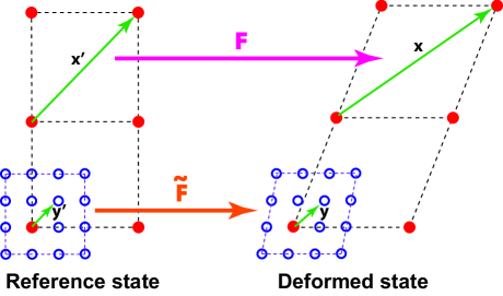
Figure 1: Dual-scale deformation of a solid material with site creation and annihilation. The marker sites (filled circles) and regular lattice sites (open circles) are connected by dashed lines to facilitate their tracking during the deformation. The shape deformation gradient $\mathbf{F}$ is defined by the motion of the markers, whereas the local lattice deformation gradient $\tilde{\mathbf{F}}$ is defined by mapping of lattice sites in the vicinity of markers. Note that the deformation of the network of markers is different from the local lattice distortion.

Since the markers are conserved during the deformation process, they can be used to define a deformation mapping $\mathbf{x}=\mathbf{x}(\mathbf{x}^{\prime},t)$ with respect to a chosen reference state, $\mathbf{x}^{\prime}$, of the material (Fig.1). This mapping defines the shape (or total) deformation gradientMalvern69

$$\mathbf{F}\equiv\left(\dfrac{\partial\mathbf{x}}{\partial\mathbf{x}^{\prime}}\right)_{t}$$ (6)

and is related to the total lattice velocity (i.e., the velocity of the marker network) by

$$\mathbf{v}_{L}=\left(\dfrac{\partial\mathbf{x}}{\partial t}\right)_{\mathbf{x}^{\prime}}.$$ (7)

If the material is crystalline, then besides $\mathbf{F}$ we can also define another lattice deformation gradient $\tilde{\mathbf{F}}$. Bilby60a To do so, we assume that for any lattice site we can identify instantaneous directions of the crystallographic axes in its vicinity. This allows us to establish a local mapping between lattice vectors, $\mathbf{y}$ and $\mathbf{y}^{\prime}$, in the current and reference states, respectively (Fig.1). The deformation gradient defined by

$$\tilde{\mathbf{F}}\equiv\left(\dfrac{\partial\mathbf{y}}{\partial\mathbf{y}^{\prime}}\right)_{\mathbf{x}^{\prime},t}$$ (8)

represents local lattice distortions in the vicinity of a marker site $\mathbf{x}^{\prime}$. It should be emphasized that this definition of $\tilde{\mathbf{F}}$ does not imply conservation of sites in the vicinity of the marker. With time, some of the sites my disappear, but their locations are then filled by other sites resulting is a self-reproduced local crystalline structure. This structure can be identified at any instant by examining the current atomic positions around the marker and establishing their mapping on the reference crystal structure. Since $\tilde{\mathbf{F}}$ is defined in a small vicinity of every marker site $\mathbf{x}^{\prime}$, we assume that it is independent of $\mathbf{y}^{\prime}$ and is a continuous function of $\mathbf{x}^{\prime}$, i.e., $\tilde{\mathbf{F}}=\tilde{\mathbf{F}}(\mathbf{x}^{\prime},t)$.

Generally, $\mathbf{F}$ and $\tilde{\mathbf{F}}$ are two different tensors. In particular, the derivative

$$\mathbf{\tilde{v}}_{L}\equiv\left(\dfrac{\partial\mathbf{y}}{\partial t}\right)_{\mathbf{x}^{\prime},\mathbf{y}^{\prime}}$$ (9)

defines the local lattice velocity $\mathbf{\tilde{v}}_{L}$ due to elastic deformation, thermal expansion and compositional strains. This velocity is generally different from the marker network velocity $\mathbf{v}_{L}$. The latter incorporates the same deformation effects as $\mathbf{\tilde{v}}_{L}$ but additionally includes the permanent deformation due to site generation and annihilation.

Thus, we introduce two different deformation gradients between the same pair of deformed and reference states of the material: the shape deformation gradient $\mathbf{F}$ defined by the marker-to-marker mapping, and the lattice deformation gradient $\tilde{\mathbf{F}}$ defined by local lattice mapping in the vicinity of every marker. The lattice site generation and annihilation during the creep process produces permanent deformation leading to deviations of $\mathbf{F}$ from $\tilde{\mathbf{F}}$. Experimentally, information about $\tilde{\mathbf{F}}$ could be obtained by X-ray diffraction measurements whereas $\mathbf{F}$ could be simultaneously measured by dilatometry. This type of measurements were used by Simmons and BalluffiSimmons1960 ; Simmons1960b to determine the equilibrium vacancy concentration in metals.

This dual description of deformation is central to our theory and will be employed for the calculations of the entropy production rate in the materials and other kinetic characteristics of diffusional creep.

There is an important kinematic relation between the two velocities $\mathbf{v}_{L}$ and $\mathbf{\tilde{v}}_{L}$, on one hand, and the lattice site production rate $r_{s}$ on the other. To derive it, return to the site balance Eq.(2). This equation can be rewritten in the form

$$\dfrac{d^{L}n_{s}}{dt}\equiv\left(\dfrac{\partial n_{s}}{\partial t}\right)_{\mathbf{x}^{\prime}}=r_{s}-n_{s}\nabla_{\mathbf{x}}\cdot\mathbf{v}_{L}.$$ (10)

On the other hand, the site density can be expressed as

$$n_{s}=\dfrac{n_{s}^{\prime}}{\tilde{G}},$$ (11)

where $\tilde{G}\equiv\det\tilde{\mathbf{F}}$ and $n_{s}^{\prime}$ is the lattice site density in the reference state, assumed to be a constant. Using the Jacobi identityMalvern69 it can be shown that

$$\dfrac{d^{L}\tilde{G}}{dt}\equiv\left(\dfrac{\partial\tilde{G}}{\partial t}\right)_{\mathbf{x}^{\prime}}=\tilde{G}\nabla_{\mathbf{y}}\cdot\mathbf{\tilde{v}}_{L},$$ (12)

where we used the local lattice mapping $\mathbf{y}=\mathbf{y}(\mathbf{y}^{\prime},\mathbf{x}^{\prime},t)$ considering the marker position $\mathbf{x}^{\prime}$ as a parameter. Applying this relation to Eq.(11) we have

$$\dfrac{d^{L}n_{s}}{dt}\equiv\left(\dfrac{\partial n_{s}}{\partial t}\right)_{\mathbf{x}^{\prime}}=n_{s}^{\prime}\left(\dfrac{\partial(1/\tilde{G})}{\partial t}\right)_{\mathbf{x}^{\prime}}=-n_{s}\nabla_{\mathbf{y}}\cdot\mathbf{\tilde{v}}_{L}.$$ (13)

There is a subtle difference between Eqs.(10) and (13). In Eq.(10), $n_{s}$ is the coarse-grained site density averaged over a volume containing a group of neighboring markers, whereas in Eq.(13) $n_{s}$ is a more detailed function of coordinates near a particular marker $\mathbf{x}^{\prime}$. Assuming that $n_{s}$ is a slowly varying function of coordinates on the scale of inter-marker distances, we treat both densities as equal and their time derivatives in Eqs.(10) and (13) as identical. This immediately gives

$$\nabla\cdot\mathbf{v}_{L}-\nabla\cdot\mathbf{\tilde{v}}_{L}=\dfrac{r_{s}}{n_{s}}.$$ (14)

We dropped the subscripts of the divergence symbols, but it should be remembered that the divergence of $\mathbf{\tilde{v}}_{L}$ is taken locally whereas the divergence of $\mathbf{v}_{L}$ is coarse-grained over a volume containing multiple markers.

Eq.(14) reflects the fact that the site generation causes deviations of the total velocity divergence $\nabla\cdot\mathbf{v}_{L}$ from the local velocity divergence $\nabla\cdot\mathbf{\tilde{v}}_{L}$ arising solely from lattice distortions. In the absence of site generation, the two velocity fields are identical and Eq.(14) correctly predicts $r_{s}=0$. We will show later that $r_{s}$ is the trace of a more general tensor representing a more complete view of the permanent deformation caused by site generation and annihilation.

III Balance equations

In this Section we summarize the momentum, energy and entropy balance relations that will be used in this work and discuss the assumptions and approximations underlying these relations.

III.1 Momentum balance

For our multicomponent system, it is necessary to derive a consistent momentum balance equation. The standard momentum equation for a single component solid, such as treated by Malvern,Malvern69 is no longer applicable because of the momentum carried by multicomponent diffusion. As shown in Appendix A, the correct momentum equation is

$$\dfrac{\partial}{\partial t}\left(\rho\mathbf{v}\right)+\nabla\cdot\left(\sum_{i=1}^{n}m_{i}n_{i}\mathbf{v}_{i}\mathbf{v}_{i}\right)=\mathbf{b}+\nabla\cdot\boldsymbol{\sigma},$$ (15)

where $\mathbf{v}$ is the barycentric velocity, $\rho$ is the material density (mass per unit volume), $\mathbf{b}=\sum_{i=1}^{n}n_{i}\mathbf{b}_{i}$ is the external force per unit volume, and $\nabla\cdot\boldsymbol{\sigma}$ is the force exerted by the stress $\boldsymbol{\sigma}$ per unit volume of the material. We assume that the external fields are conservative, so that the force per particle

$$\mathbf{b}_{i}=-\nabla\psi_{i},$$ (16)

where $\psi_{i}$ are species-specific potential functions.

Eq.(15) can be rewritten with respect to the lattice (see Appendix A)

$$\rho\dfrac{d^{L}\mathbf{v}_{L}}{dt}=\mathbf{b}+\nabla\cdot\left(\boldsymbol{\sigma}-\mathbf{M}\right)-\dfrac{d^{L}\boldsymbol{q}}{dt}-\boldsymbol{q}\nabla\cdot\mathbf{v}_{L}-\boldsymbol{q}\cdot\nabla\mathbf{v}_{L},$$ (17)

where tensor $\mathbf{M}$ is given by

$$\mathbf{M}\equiv\sum_{i=1}^{n}\dfrac{m_{i}}{n_{i}}\mathbf{J}_{i}^{L}\mathbf{J}_{i}^{L}$$ (18)

and vector

$$\boldsymbol{q}\equiv\sum_{i=1}^{n}m_{i}\mathbf{J}_{i}^{L}=\rho\left(\mathbf{v}-\mathbf{v}_{L}\right)$$ (19)

is the momentum density carried by the local center of mass relative to the lattice. Here, $m_{i}$ is the mass of particles of species $i$. The derivative $d^{L}\boldsymbol{q}/dt$ is the inertia force which arises due to the fact that the lattice and barycentric references are both non-inertial.

III.2 Energy balance

The total energy $e$ of the material per unit volume can be expressed

$$e=K+\psi+u.$$ (20)

where

$$K=\dfrac{1}{2}\sum_{i=1}^{n}m_{i}n_{i}|\mathbf{v}_{i}|^{2}$$ (21)

is the macroscopic kinetic energy of the particles per unit volume,

$$\psi\equiv\sum_{i=1}^{n}n_{i}\psi_{i}$$ (22)

is potential energy in external fields per unit volume, and the remaining term $u$ is identified with internal energy per unit volume. The latter includes the energy of interactions between the particles and the kinetic energy of their microscopic motion (e.g., lattice vibrations, molecular rotations, etc.), but excludes the macroscopic kinetic energy due to diffusion. The internal energy can be shown to satisfy the following balance equation with respect to the lattice (see Appendix A):

$$\dfrac{d^{L}u}{dt}+u\nabla\cdot\mathbf{v}_{L} = -\nabla\cdot\mathbf{J}_{u}^{L}+\sum_{i=1}^{n}\mathbf{b}_{i}\cdot\mathbf{J}_{i}^{L}+\left(\boldsymbol{\sigma}-\mathbf{M}\right):\nabla\mathbf{v}_{L}$$ (23)

$$-\sum_{i=1}^{n}\left\{\nabla\left[\dfrac{m_{i}}{2n_{i}^{2}}\left(\mathbf{J}_{i}^{L}\cdot\mathbf{J}_{i}^{L}\right)\right]+m_{i}\dfrac{d^{L}\mathbf{v}_{i}}{dt}\right\}\cdot\mathbf{J}_{i}^{L},$$

where $\mathbf{J}_{u}^{L}$ is the internal energy flux relative to the lattice.

Equation (23) is valid for all, not necessarily reversible, process and expresses the first law of thermodynamics stating that the change in internal energy equals the work done on the system less the energy dissipated through its boundaries. As with the momentum balance relation (17), Eq.(23) is exact: it represents the internal energy balance without any approximations or assumptions other than the conservation of energy and the total energy ansatz (20).

We will also need the potential energy balance relation,

$$\dfrac{d^{L}\psi}{dt}+\psi\nabla\cdot\mathbf{v}_{L}=-\sum_{i=1}^{n}\mathbf{b}_{i}\cdot\mathbf{J}_{i}^{L}-\mathbf{b}\cdot\mathbf{v}_{L}-\nabla\cdot\left(\sum_{i=1}^{n}\psi_{i}\mathbf{J}_{i}^{L}\right),$$ (24)

where the last term represents the divergence of the diffusive flux of potential energy. This relation is also exact.

III.3 Entropy balance

The entropy balance is postulated in the form

$$\dfrac{d^{L}s}{dt}+s\nabla\cdot\mathbf{v}_{L}+\nabla\cdot\mathbf{J}_{s}^{L}=\dot{s},$$ (25)

where $s$ is entropy per unit volume, $\mathbf{J}_{s}^{L}$ is the entropy flux carried by the conduction of heat relative to the lattice, and $\dot{s}$ is the entropy production rate due to irreversible processes.

The goal of the subsequent development will be to compute $\dot{s}$. The common approachDe-Groot1984 to achieving this goal is to calculate the entropy rate $(d^{L}s/dt+s\nabla\cdot\mathbf{v}_{L})$ and then rearrange the terms to form the divergence of fluxes that can be identified with $-\nabla\cdot\mathbf{J}_{s}^{L}$. The remaining terms are then identified with $\dot{s}$. We will follow this route to derive $\dot{s}$ for a solid material containing non-conserved lattice sites.

IV Local reversible thermodynamics

IV.1 The local equilibrium postulate

It is assumed that, although the entire solid material can be away from equilibrium, its local internal energy, entropy and other thermodynamic variables are related to each other via a fundamental equation of state describing reversible processes. “Local” means here that this equation is followed only by subsystems of the entire system that are small enough to reach thermodynamic equilibrium before the entire system does, yet large enough to apply the full formalism of thermodynamics. The locally equilibrium subsystems need not be uniform and can be treated using the formalism of gradient thermodynamics.Bloch1932 ; Ginzburg1950 ; Cahn58a

Relative to the moving lattice, the fundamental equation is postulated in the functional form:

$$u=u\left(s,\{n_{i}\},\{\varphi_{k}\},\{\nabla n_{i}\},\{\nabla\varphi_{k}\},\tilde{\mathbf{F}}\right).$$ (26)

Here, $\varphi_{k}$ ($k=1,...,K$) are non-conserved phase fields, $\nabla n_{i}$ and $\nabla\varphi_{k}$ are respective gradients, and $\tilde{\mathbf{F}}$ is the lattice deformation gradient relative to a chosen reference state (Sec. II). The phase fields $\varphi_{k}$ can represent different thermodynamic phases of the material or be associated with different lattice orientations (grains) in a single-phase polycrystalline material. The gradients $\nabla\varphi_{k}$ and $\nabla n_{i}$ are usually negligibly small inside the bulk phases or grains but are important in the description of inter-phase interfaces and GBs. The material regions whose thermodynamic description requires the gradientsBloch1932 ; Ginzburg1950 ; Cahn58a are referred to as “non-classical” as opposed to “classical” regions which can be treated within the standard thermodynamicsWillard_Gibbs of homogeneous phases. Since $u$ is a scalar while the gradients are vectors and $\tilde{\mathbf{F}}$ is a tensor, it is assumed that Eq.(26) satisfies the required invariance under rotations of the coordinate system.

When Eq.(26) is applied to different locations in the solid, it is assumed that the reference state used to describe the lattice deformation is the same for every location and is fixed once and for all. For example, for a cubic crystal the reference state can be a perfectly cubic unit cell with a given (e.g., stress-free) lattice constant. This explains why properties of the reference state, such as the reference volume per site, are not listed among the variables of $u$.

IV.2 The first and second laws of thermodynamics for local reversible processes

To derive the differential form of Eq.(26), let us first consider a uniform region containing a fixed number of lattice sites. Suppose for the moment that the phase fields $\varphi_{k}$ are not included. The standard differential form of the fundamental equation for such a region is

$$dU=TdS+\sum_{i=1}^{n}M_{i}dN_{i}+V\left(\tilde{\mathbf{F}}^{-1}\cdot\tilde{\mathbf{\boldsymbol{\sigma}}}\right)\cdot\cdot d\tilde{\mathbf{F}}.$$ (27)

Here $U=uV$, $S=sV$ and $N_{i}=n_{i}V$ are the total internal energy, entropy and numbers of particles of the chemical components inside the region, $V$ is its volume, $T\equiv\partial U/\partial S$ is temperature and $\tilde{\mathbf{F}}^{-1}$ is the inverse of $\tilde{\mathbf{F}}$. The tensor $\tilde{\mathbf{\boldsymbol{\sigma}}}$ is formally defined through the derivative $\partial U/\partial\mathbf{\tilde{\mathbf{F}}}$,

$$\tilde{\mathbf{\boldsymbol{\sigma}}}\equiv\dfrac{1}{V}\mathbf{\tilde{\mathbf{F}}}\cdot\dfrac{\partial U}{\partial\mathbf{\tilde{\mathbf{F}}}},$$ (28)

and has the meaning of the equilibrium Cauchy stress in a uniform lattice. As will be discussed later, $\tilde{\mathbf{\boldsymbol{\sigma}}}$ it is generally different from the actual stress tensor $\boldsymbol{\sigma}$ in a non-uniform and/or non-equilibrium material. The obvious motivation behind the definition (28) is the standard form $V^{\prime}\mathbf{P}\cdot\cdot d\tilde{\mathbf{F}}$ of the mechanical work term in continuum mechanicsMalvern69 , $V^{\prime}$ being the reference volume of the region and $\mathbf{P}=\tilde{J}\tilde{\mathbf{F}}^{-1}\cdot\tilde{\mathbf{\boldsymbol{\sigma}}}$ the first Piola-Kirchhoff stress tensor. Finally, the derivative $M_{i}\equiv\partial U/\partial N_{i}$ has the meaning of the diffusion potential of species $i$ relative to vacancies if the latter are treated as massless species. If only the material particles are treated as species, $M_{i}$ can be considered as simply the chemical potential of species $i$. As discussed in the literatureLarche1985 ; Mullins1985 , both interpretations of $M_{i}$ are equally legitimate and give the same results for all physically observable quantities.

Eq.(27) can be rewritten in terms of the volume densities $u$, $s$ and $n_{i}$ :

$$du=Tds+\sum_{i=1}^{n}M_{i}dn_{i}+\left(\tilde{\mathbf{F}}^{-1}\cdot\tilde{\mathbf{\boldsymbol{\sigma}}}\right)\cdot\cdot d\tilde{\mathbf{F}}-\left(u-Ts-\sum_{i=1}^{n}M_{i}n_{i}\right)\dfrac{dV}{V}.$$ (29)

Using the identityMalvern69

$$\dfrac{dV}{V}=\tilde{\mathbf{F}}^{-1}\cdot\cdot d\tilde{\mathbf{F}}$$ (30)

we obtain

$$du=Tds+\sum_{i=1}^{n}M_{i}dn_{i}+\left(\tilde{\mathbf{F}}^{-1}\cdot\left(\tilde{\mathbf{\boldsymbol{\sigma}}}-\omega\mathbf{I}\right)\right)\cdot\cdot d\tilde{\mathbf{F}},$$ (31)

where $\mathbf{I}$ is the second rank unit tensor and

$$\omega\equiv u-Ts-\sum_{i=1}^{n}M_{i}n_{i}$$ (32)

is the grand-canonical potential per unit volume.

Eq.(31) is the differential form of Eq.(26) for the particular case of a uniform material without phase fields. In the presence of phase fields and the gradients $\nabla\varphi_{k}$ and $\nabla n_{i}$, this equation becomes

$$du = Tds+\sum_{i=1}^{n}M_{i}dn_{i}+\sum_{k=1}^{K}\dfrac{\partial u}{\partial\varphi_{k}}d\varphi_{k}+\sum_{i=1}^{n}\dfrac{\partial u}{\partial\nabla n_{i}}\cdot d\nabla n_{i}+\sum_{k=1}^{K}\dfrac{\partial u}{\partial\nabla\varphi_{k}}\cdot d\nabla\varphi_{k}$$ (33)

$$+ \left(\tilde{\mathbf{F}}^{-1}\cdot\left(\tilde{\mathbf{\boldsymbol{\sigma}}}-\omega\mathbf{I}\right)\right)\cdot\cdot d\tilde{\mathbf{F}}.$$

Note that $\omega$ appearing in the last term is now a non-classical quantity as it depends on the gradients through $u$ [cf. Eq.(26)].

The gradient terms in Eq.(33) can be rearranged using the identities

$$\sum_{i=1}^{n}\dfrac{\partial u}{\partial\nabla n_{i}}\cdot d\nabla n_{i} = \sum_{i=1}^{n}\nabla\cdot\left(\dfrac{\partial u}{\partial\nabla n_{i}}dn_{i}\right)-\sum_{i=1}^{n}\left(\nabla\cdot\dfrac{\partial u}{\partial\nabla n_{i}}\right)dn_{i}$$

$$+ \sum_{i=1}^{n}\dfrac{\partial u}{\partial\nabla n_{i}}\cdot\left(d\nabla n_{i}-\nabla dn_{i}\right),$$

$$\sum_{k=1}^{K}\dfrac{\partial u}{\partial\nabla\varphi_{k}}\cdot d\nabla\varphi_{k} = \sum_{k=1}^{K}\nabla\cdot\left(\dfrac{\partial u}{\partial\nabla\varphi_{k}}d\varphi_{k}\right)-\sum_{k=1}^{K}\left(\nabla\cdot\dfrac{\partial u}{\partial\nabla\varphi_{k}}\right)d\varphi_{k}$$ (35)

$$+ \sum_{k=1}^{K}\dfrac{\partial u}{\partial\nabla\varphi_{k}}\cdot\left(d\nabla\varphi_{k}-\nabla d\varphi_{k}\right),$$

where we recognize that the operations $d$ and $\nabla$ may not commute. Equation (33) finally becomes

$$du = Tds+\sum_{i=1}^{n}M_{i}^{*}dn_{i}+\sum_{k=1}^{K}\Phi_{k}^{*}d\varphi_{k}+\nabla\cdot\left(\sum_{i=1}^{n}\dfrac{\partial u}{\partial\nabla n_{i}}dn_{i}+\sum_{k=1}^{K}\dfrac{\partial u}{\partial\nabla\varphi_{k}}d\varphi_{k}\right)$$ (36)

$$+ \sum_{i=1}^{n}\dfrac{\partial u}{\partial\nabla n_{i}}\cdot\left(d\nabla n_{i}-\nabla dn_{i}\right)+\sum_{k=1}^{K}\dfrac{\partial u}{\partial\nabla\varphi_{k}}\cdot\left(d\nabla\varphi_{k}-\nabla d\varphi_{k}\right)$$

$$+ \left(\tilde{\mathbf{F}}^{-1}\cdot\left(\tilde{\mathbf{\boldsymbol{\sigma}}}-\omega\mathbf{I}\right)\right)\cdot\cdot d\tilde{\mathbf{F}},$$

where

$$M_{i}^{*}\equiv\dfrac{\partial u}{\partial n_{i}}-\nabla\cdot\dfrac{\partial u}{\partial\nabla n_{i}}=M_{i}-\nabla\cdot\dfrac{\partial u}{\partial\nabla n_{i}}$$ (37)

is the non-classical diffusion potential and

$$\Phi_{k}^{*}\equiv\dfrac{\partial u}{\partial\varphi_{k}}-\nabla\cdot\dfrac{\partial u}{\partial\nabla\varphi_{k}}.$$ (38)

Note that $M_{i}^{*}$ and $\Phi_{k}^{*}$ are variational derivativesGelfand-Fomin of the internal energy with respect to the concentrations $n_{i}$ and phase fields $\varphi_{k}$, respectively.

The obtained Eq.(36) is a formulation of the first and second laws of thermodynamics for local reversible processes in a lattice obeying the fundamental equation (26). It will serve as the starting point for several derivations performed below.

IV.3 Generalized Gibbs-Duhem equation

By applying a partial Legendre transformation Gelfand-Fomin with respect to $s$ and $n_{i}$, Eq.(36) can be transformed to

$$sdT+\sum_{i=1}^{n}n_{i}dM_{i}^{*}+d\omega-\sum_{k=1}^{K}\Phi_{k}^{*}d\varphi_{k}+\sum_{i=1}^{n}d\left(n_{i}\nabla\cdot\dfrac{\partial u}{\partial\nabla n_{i}}\right)$$

$$-\nabla\cdot\left(\sum_{i=1}^{n}\dfrac{\partial u}{\partial\nabla n_{i}}dn_{i}+\sum_{k=1}^{K}\dfrac{\partial u}{\partial\nabla\varphi_{k}}d\varphi_{k}\right)$$

$$-\sum_{i=1}^{n}\dfrac{\partial u}{\partial\nabla n_{i}}\cdot\left(d\nabla n_{i}-\nabla dn_{i}\right)-\sum_{k=1}^{K}\dfrac{\partial u}{\partial\nabla\varphi_{k}}\cdot\left(d\nabla\varphi_{k}-\nabla d\varphi_{k}\right)$$

$$-\left(\tilde{\mathbf{F}}^{-1}\cdot\left(\tilde{\mathbf{\boldsymbol{\sigma}}}-\omega\mathbf{I}\right)\right)\cdot\cdot d\tilde{\mathbf{F}}=0.$$ (39)

This equation can be viewed as a generalization of the Gibbs-Duhem equationWillard_Gibbs to a non-classical solid subject to non-hydrostatic mechanical stresses. In the particular case of a hydrostatically stressed classical (no gradients) solid we have $\tilde{\mathbf{\boldsymbol{\sigma}}}=-p\mathbf{I}$, where $p=-\omega$ is the equilibrium hydrostatic pressure, and Eq.(39) reduces to the standard Gibbs-Duhem equationWillard_Gibbs

$$sdT+\sum_{i=1}^{n}n_{i}dM_{i}-dp=0.$$ (40)

As an application of Eq.(39), suppose the differentials represent infinitesimal differences between the values of properties at two nearby points $\mathbf{x}$ and $\mathbf{x}+d\mathbf{x}$ at a fixed moment of time. Then $dT=\nabla T\cdot d\mathbf{x}$, $dM_{i}^{*}=\nabla M_{i}^{*}\cdot d\mathbf{x}$, and similarly for all other terms. In this particular case the operators $d$ and $\nabla$ commute, $\nabla d=d\nabla=d\mathbf{x}\cdot\nabla\nabla$, and both sums in the third line of Eq.(39) vanish. The remaining terms contain the common factor $d\mathbf{x}$ which cancels, giving

$$s\nabla T+\sum_{i=1}^{n}n_{i}\nabla M_{i}^{*}-\sum_{k=1}^{K}\Phi_{k}^{*}\nabla\varphi_{k}+\nabla\cdot\left(\mathbf{A}^{*}+\omega\mathbf{I}\right)-\left(\tilde{\mathbf{F}}^{-1}\cdot\left(\tilde{\mathbf{\boldsymbol{\sigma}}}-\omega\mathbf{I}\right)\right)\cdot\cdot\left(\tilde{\mathbf{F}}\overleftarrow{\nabla}\right)=0,$$ (41)

where

$$\mathbf{A^{*}}\equiv\left(\sum_{i=1}^{n}n_{i}\nabla\cdot\dfrac{\partial u}{\partial\nabla n_{i}}\right)\mathbf{I}-\sum_{i=1}^{n}\dfrac{\partial u}{\partial\nabla n_{i}}\nabla n_{i}-\sum_{k=1}^{K}\dfrac{\partial u}{\partial\nabla\varphi_{k}}\nabla\varphi_{k}$$ (42)

is a purely non-classical second-rank tensor.

Equation (41) is a gradient form of the generalized Gibbs-Duhem equation (39). As will be shown later (Sec. V), when the material reaches full thermodynamic equilibrium (including equilibrium with respect to site generation and annihilation), the first, third and last terms in Eq.(41) vanish while the non-classical chemical potentials satisfy the condition $\nabla M_{i}^{*}-\mathbf{b}_{i}=\mathbf{0}.$ It follows that under the full equilibrium conditions

$$\nabla\cdot\left(\mathbf{A}^{*}+\omega\mathbf{I}\right)+\mathbf{b}=\mathbf{0}.$$ (43)

Thus, in the absence of external fields, tensor $\left(\mathbf{A}^{*}+\omega\mathbf{I}\right)$ is divergence-free. In a one-dimensional system this means conservation of the quantity $(A_{11}^{*}+\omega)$.

The divergence-free character of $\left(\mathbf{A}^{*}+\omega\mathbf{I}\right)$ in the absence of external fields originates from the property of the fundamental equation (26) that the internal energy does not depend explicitly on the position vector $\mathbf{x}$. If it did, an additional term $\partial u/\partial\mathbf{x}$ would appear in Eq.(33) and eventually propagate to Eq.(43), so that the divergence of $\left(\mathbf{A}^{*}+\omega\mathbf{I}\right)$ would no longer be zero. The mathematical procedure that produced the divergence term in Eqs.(41) and (43) is essentially equivalent to a derivation of Noether’s theorem Gelfand-Fomin for a system with continuous translational symmetry. Applied fields $\mathbf{b}_{i}$ obviously destroy this symmetry and lead to a nonzero divergence of $\left(\mathbf{A}^{*}+\omega\mathbf{I}\right)$ as indicated in Eq.(43).

IV.4 Time-dependent form of the first and second laws

Returning to the general Eq.(36), we now consider the case where the differentials represent changes in time. Because the internal energy $u$ has been defined relative to the stationary lattice, its time evolution must be described by the lattice material derivative $d^{L}u/dt$ defined by Eq.(5). We will therefore interpret all differentials $d$ in Eq.(36) as $d^{L}/dt$.

The operators $d^{L}/dt$ and $\nabla$ do not commute, but it can be shown that

$$\dfrac{d^{L}}{dt}\nabla-\nabla\dfrac{d^{L}}{dt}=-\nabla\mathbf{v}_{L}\cdot\nabla.$$ (44)

As a result, the second line in Eq.(36) becomes

$$-\sum_{i=1}^{n}\dfrac{\partial u}{\partial\nabla n_{i}}\cdot\nabla\mathbf{v}_{L}\cdot\nabla n_{i}-\sum_{k=1}^{K}\dfrac{\partial u}{\partial\nabla\varphi_{k}}\cdot\nabla\mathbf{v}_{L}\cdot\nabla\varphi_{k}$$

and can be simplified to

$$-\left(\sum_{i=1}^{n}\dfrac{\partial u}{\partial\nabla n_{i}}\nabla n_{i}+\sum_{k=1}^{K}\dfrac{\partial u}{\partial\nabla\varphi_{k}}\nabla\varphi_{k}\right):\nabla\mathbf{v}_{L}.$$

The last term in Eq.(36) can be transformed to

$$\left(\tilde{\mathbf{F}}^{-1}\cdot\left(\tilde{\mathbf{\boldsymbol{\sigma}}}-\omega\mathbf{I}\right)\right)\cdot\cdot\dfrac{d^{L}\tilde{\mathbf{F}}}{dt}=\left(\tilde{\mathbf{\boldsymbol{\sigma}}}-\omega\mathbf{I}\right):\nabla\mathbf{\tilde{v}}_{L},$$

where we used the identity

$$\dfrac{d^{L}\tilde{\mathbf{F}}}{dt}=\left(\mathbf{\tilde{v}}_{L}\overleftarrow{\nabla}\right)\cdot\tilde{\mathbf{F}}.$$ (45)

Eq.(36) becomes

$$\dfrac{d^{L}u}{dt} = T\dfrac{d^{L}s}{dt}+\sum_{i=1}^{n}M_{i}^{*}\dfrac{d^{L}n_{i}}{dt}+\sum_{k=1}^{K}\Phi_{k}^{*}\dfrac{d^{L}\varphi_{k}}{dt}+\nabla\cdot\left(\sum_{i=1}^{n}\dfrac{\partial u}{\partial\nabla n_{i}}\dfrac{d^{L}n_{i}}{dt}+\sum_{k=1}^{K}\dfrac{\partial u}{\partial\nabla\varphi_{k}}\dfrac{d^{L}\varphi_{k}}{dt}\right)$$ (46)

$$- \left(\sum_{i=1}^{n}\dfrac{\partial u}{\partial\nabla n_{i}}\nabla n_{i}+\sum_{k=1}^{K}\dfrac{\partial u}{\partial\nabla\varphi_{k}}\nabla\varphi_{k}\right):\nabla\mathbf{v}_{L}+\left(\tilde{\mathbf{\boldsymbol{\sigma}}}-\omega\mathbf{I}\right):\nabla\mathbf{\tilde{v}}_{L}.$$

Note that this equation contains both the total (marker network) velocity and the local velocity of the lattice, the former coming from the material time derivatives and the latter from the local lattice deformation gradient.

The term with the chemical potentials can be further rearranged using the species conservation law, Eq.(5):

$$\sum_{i=1}^{n}M_{i}^{*}\dfrac{dn_{i}}{dt} = -\sum_{i=1}^{n}M_{i}^{*}\nabla\cdot\mathbf{J}_{i}^{L}-\left(\sum_{i=1}^{n}M_{i}^{*}n_{i}\right)\nabla\cdot\mathbf{v}_{L}$$ (47)

$$= -\nabla\cdot\left(\sum_{i=1}^{n}M_{i}^{*}\mathbf{J}_{i}^{L}\right)+\sum_{i=1}^{n}\mathbf{J}_{i}^{L}\cdot\nabla M_{i}^{*}-\left(\sum_{i=1}^{n}M_{i}^{*}n_{i}\right)\nabla\cdot\mathbf{v}_{L}.$$

For further calculations we need the energy and entropy rates to appear in the combinations $(d^{L}u/dt+u\nabla\cdot\mathbf{v}_{L})$ and $(d^{L}s/dt+s\nabla\cdot\mathbf{v}_{L})$, respectively. This is readily achieved by adding and subtracting $u\nabla\cdot\mathbf{v}_{L}$ and $s\nabla\cdot\mathbf{v}_{L}$ in Eq.(46). After simple rearrangements we arrive at the equation

$$\dfrac{d^{L}u}{dt}+u\nabla\cdot\mathbf{v}_{L}= T\left(\dfrac{d^{L}s}{dt}+s\nabla\cdot\mathbf{v}_{L}\right)+\sum_{i=1}^{n}\mathbf{J}_{i}^{L}\cdot\nabla M_{i}^{*}+\sum_{k=1}^{K}\Phi_{k}^{*}\dfrac{d^{L}\varphi_{k}}{dt}$$ (48)

$$+\nabla\cdot\left(\sum_{i=1}^{n}\dfrac{\partial u}{\partial\nabla n_{i}}\dfrac{d^{L}n_{i}}{dt}+\sum_{k=1}^{K}\dfrac{\partial u}{\partial\nabla\varphi_{k}}\dfrac{d^{L}\varphi_{k}}{dt}-\sum_{i=1}^{n}M_{i}^{*}\mathbf{J}_{i}^{L}\right)$$

$$+\left(\tilde{\mathbf{\boldsymbol{\sigma}}}+\mathbf{A}^{*}\right):\nabla\mathbf{v}_{L}-\left(\tilde{\mathbf{\boldsymbol{\sigma}}}-\omega\mathbf{I}\right):\mathbf{R},$$

where

$$\mathbf{R}\equiv\left(\nabla\mathbf{v}_{L}-\nabla\mathbf{\tilde{v}}_{L}\right).$$ (49)

The tensor $\mathbf{R}$ represents the permanent part of the total deformation rate coming from the site generation and annihilation. According to Eq.(14) its trace,

$$\textrm{Tr}(\mathbf{R})=\left(\nabla\cdot\mathbf{v}_{L}-\nabla\cdot\mathbf{\tilde{v}}_{L}\right)=\dfrac{r_{s}}{n_{s}},$$ (50)

gives the site generation rate $r_{s}$. However, the tensor $\mathbf{R}$ carries more information than $r_{s}$ as it reflects the possible anisotropy in the generation of lattice sites. It differentiates, for example, between insertion of new lattice planes normal to a certain direction and creation of the same number of sites by uniform “swelling” of the material. In fact, $\mathbf{R}$ captures even a pure shear deformation rate in which new lattice planes are inserted parallel to one crystallographic orientation and simultaneously removed parallel to another crystallographic orientation perpendicular to the first, so that the total number of sites remains constant. One possible mechanism of this process would be a concurrent climb of two perpendicular sets of edge dislocations, one inserting lattice planes and the other eliminating perpendicular lattice planes. This could be accomplished by vacancy diffusion between the cores of the two dislocation sets without changing the net amount of vacancies in the region.

Tensor $\mathbf{R}$ is related to the generalized creep strain-rate tensor $\boldsymbol{\varepsilon}_{gc}$ introduced by Svoboda et al.Svoboda2006 ; Fischer2011 although the latter, by contrast to $\mathbf{R}$, comprises both permanent and elastic parts of the deformation. Similar to $\mathbf{R}$, the tensor $\boldsymbol{\varepsilon}_{gc}$ includes both the volume creep deformation by “swelling” or contraction and shear deformation arising due to orientational anisotropy of the microstructure or from non-hydrostatic components of the stress tensor.

It should be emphasized that Eq.(48) has been derived from the fundamental Eq.(26) by a chain of mathematical transformations without any additional physical assumptions or approximations other than the conservation and balance equations of Secs. II and III. Equation (48) represents a time-dependent form of the first and second laws of thermodynamics for reversible processes in a continuous medium with the postulated equation of state (26).

V The state of equilibrium

V.1 Derivation of equilibrium conditions

Before analyzing irreversible processes, we will derive the conditions of thermodynamic equilibrium of a multicomponent solid capable of site generation. This could be done by requiring that the first-order variation of the total energy of a given material region enclosed in a rigid envelope be zero under the constraints of fixed entropy and fixed total number of particles of every species. Instead of considering infinitesimal variations of the relevant parameters, we will reuse Eq.(48) by treating the rates of the reversible changes of those parameters as their variations. For example, the variation $\delta\varphi_{k}$ can be formally considered to occur per unit time and be represented by the material derivative $d^{L}\varphi_{k}/dt$. Likewise, the virtual lattice displacement $\delta\mathbf{x}_{L}$ can be thought of as occurring per unit time and be replaced by the lattice velocity $\mathbf{v}_{L}$. The macroscopic kinetic energy is a second-order variation and is excluded. This treatment is completely equivalent to the virtual displacement method usually applied for finding thermodynamic equilibrium of continuous media.Malvern69 ; Larche73 ; Voorhees2004

The equilibrium condition is

$$\int\left(\dfrac{d^{L}u}{dt}+u\nabla\cdot\mathbf{v}_{L}\right)dV+\int\left(\dfrac{d^{L}\psi}{dt}+\psi\nabla\cdot\mathbf{v}_{L}\right)dV-\lambda\int\left(\dfrac{d^{L}s}{dt}+s\nabla\cdot\mathbf{v}_{L}\right)dV=0.$$ (51)

The first integral is equivalent to

$$\int\left(\dfrac{\partial u^{\prime}}{\partial t}\right)_{\mathbf{x}^{\prime}}dV^{\prime},$$ (52)

$u^{\prime}$ being internal entropy per unit reference volume, and represents the rate of internal energy change of a given material region defined by lattice markers. Likewise, the second and third integrals represent the rates of potential energy and entropy changes of the same material region. The entropy integral has been added to impose the entropy constraint using the Lagrange multiplier $\lambda$. The required conservation of the total amount of each species will be enforced by zero normal components of the diffusion fluxes at the boundary of the region and need not be imposed via additional Lagrange multipliers.

Inserting the first integrand from Eq.(48), the divergence term becomes the surface integral over the boundary of the region,

$$\int\mathbf{n}\cdot\left(\sum_{i=1}^{n}\dfrac{\partial u}{\partial\nabla n_{i}}\dfrac{d^{L}n_{i}}{dt}+\sum_{k=1}^{K}\dfrac{\partial u}{\partial\nabla\varphi_{k}}\dfrac{d^{L}\varphi_{k}}{dt}-\sum_{i=1}^{n}M_{i}^{*}\mathbf{J}_{i}^{L}\right)dA,$$ (53)

$\mathbf{n}$ being a unit normal vector pointing outside the region and $dA$ an increment of area. To ensure that the region is closed, the normal components of the diffusion fluxes will be taken to be zero, $\mathbf{n}\cdot\mathbf{J}_{i}^{L}=0$. Imposing also fixed boundary values of $n_{i}$ and $\varphi_{k}$, this surface integral vanishes. Furthermore, the volume integral

$$\int\left(\tilde{\mathbf{\boldsymbol{\sigma}}}+\mathbf{A}^{*}\right):\nabla\mathbf{v}_{L}dV$$ (54)

can be rewritten using the divergence theorem as

$$\int\mathbf{n}\cdot\left(\tilde{\mathbf{\boldsymbol{\sigma}}}+\mathbf{A}^{*}\right)\cdot\mathbf{v}_{L}dA-\int\nabla\cdot\left(\tilde{\mathbf{\boldsymbol{\sigma}}}+\mathbf{A}^{*}\right)\cdot\mathbf{v}_{L}dV,$$ (55)

where the surface integral is zero due to the boundary condition $\mathbf{v}_{L}=\mathbf{0}$ (rigid boundary). Similarly, per Eq.(24) the potential energy integral contains the potential energy flux which vanishes on the boundary, leaving

$$\int\left(\dfrac{d^{L}\psi}{dt}+\psi\nabla\cdot\mathbf{v}_{L}\right)dV=-\int\left(\sum_{i=1}^{n}\mathbf{b}_{i}\cdot\mathbf{J}_{i}^{L}+\mathbf{b}\cdot\mathbf{v}_{L}\right)dV.$$ (56)

Combining the above equations, Eq.(51) becomes

$$\int\left(\dfrac{d^{L}s}{dt}+s\nabla\cdot\mathbf{v}_{L}\right)(T-\lambda)dV+\int\sum_{i=1}^{n}\mathbf{J}_{i}^{L}\cdot\nabla\left(M_{i}^{*}+\psi_{i}\right)dV+\int\sum_{k=1}^{K}\Phi_{k}^{*}\dfrac{d^{L}\varphi_{k}}{dt}dV$$

$$-\int\left[\nabla\cdot\left(\tilde{\mathbf{\boldsymbol{\sigma}}}+\mathbf{A}^{*}\right)+\mathbf{b}\right]\cdot\mathbf{v}_{L}dV-\int\left(\tilde{\mathbf{\boldsymbol{\sigma}}}-\omega\mathbf{I}\right):\mathbf{R}dV=0.$$ (57)

In the state of equilibrium this relation must hold for any arbitrarily chosen region of the material. The integrands are proportional to the entropy rate $(d^{L}s/dt+s\nabla\cdot\mathbf{v}_{L})$, the phase-field rates $d^{L}\varphi_{k}/dt$, the diffusion fluxes $\mathbf{J}_{i}^{L}$, the lattice velocity $\mathbf{v}_{L}$, and the creep deformation rate $\mathbf{R}$, respectively. All these rates represent independent variations away from the equilibrium state. Assuming that they can take any arbitrary positive or negative values, the coefficients multiplying these rates must be zero. We thus arrive at the following set of necessary conditions of equilibrium:

$$T=\lambda=\textnormal{const}\quad\quad\textnormal{Thermal equilibrium}$$ (58)

$$M_{i}^{*}+\psi_{i}=\textnormal{const}\quad\quad\textnormal{Chemical equilibrium }$$ (59)

$$\Phi_{k}^{*}=0\quad\quad\textnormal{Phase-field equilibrium }$$ (60)

$$\nabla\cdot\left(\tilde{\mathbf{\boldsymbol{\sigma}}}+\mathbf{A}^{*}\right)+\mathbf{b}=0\quad\quad\textnormal{Mechanical equilibrium }$$ (61)

$$\tilde{\mathbf{\boldsymbol{\sigma}}}=\omega\mathbf{I}.\quad\quad\textnormal{Site generation equilibrium }$$ (62)

V.2 Discussion of the equilibrium conditions

Eqs.(58)-(60) reproduce the well-known conditions of thermal, chemical and phase field equilibrium: the uniformity of the temperature field, the constancy of the non-classical chemical potential $M_{i}^{*}$ plus the external potential $\psi_{i}$ for every species, and vanishing variational derivative $\Phi_{k}^{*}$ for every phase field.

The mechanical equilibrium condition could have been obtained from zero accelerations and zero diffusion fluxes in the momentum balance equation (17), giving $\nabla\cdot\boldsymbol{\sigma}+\mathbf{b}=\mathbf{0}$. Equation (61) shows that tensor $(\tilde{\mathbf{\boldsymbol{\sigma}}}+\mathbf{A}^{*})$ plays the role of the non-classical stress tensor. The latter has long been known in fluid systems as the capillary tensor or Korteweg stress.Korteweg1901 In classical regions where the gradients of the chemical composition and phase fields can be neglected and thus $\mathbf{\mathbf{A}^{*}}=\mathbf{0}$, the mechanical equilibrium condition reduces to $\nabla\cdot\tilde{\mathbf{\boldsymbol{\sigma}}}+\mathbf{b}=\mathbf{0}$, confirming that the tensor $\tilde{\mathbf{\boldsymbol{\sigma}}}$ defined earlier by Eq.(28) is indeed the equilibrium stress tensor in a classical solid.

Equation (62) is the condition of equilibrium with respect to site generation and annihilation, stating that tensor $\tilde{\mathbf{\boldsymbol{\sigma}}}$ must be diagonal: $\tilde{\mathbf{\boldsymbol{\sigma}}}\equiv-p\mathbf{I}$. This condition must be fulfilled everywhere in the equilibrium material, including non-classical regions with significant gradients of $n_{i}$ and/or $\varphi_{k}$, such as interface regions. However, the actual stress tensor in such regions, $(-p\mathbf{I}+\mathbf{A}^{*})$, remains non-hydrostatic due to the non-classical contribution $\mathbf{A}^{*}$.

If Eq.(62) is satisfied, the mechanical equilibrium condition becomes

$$-\nabla p+\nabla\cdot\mathbf{A}^{*}+\mathbf{b}=\mathbf{0}$$ (63)

and in classical regions reduces to the standard hydrostatic equilibrium condition $\nabla p=\mathbf{b}$.Malvern69 Thus, in the presence of efficient sinks and sources of vacancies capable of maintaining site equilibrium the solid behaves rheologically like a fluid.

Note that by inserting the obtained equilibrium conditions (58)-(60) and (62) in the generalized Gibbs-Duhem equation (41) we immediately recover Eq.(43) or its equivalent form (63). In other words, if all other equilibrium conditions are satisfied, the mechanical equilibrium condition follows from the generalized Gibbs-Duhem equation (41). The reverse is not true: the mechanical equilibrium condition (61) can be satisfied even if the material has not reached complete equilibrium, in which case Eq.(43) is invalid.

According to Eq.(62), in equilibrium $p=-\omega$, i.e.,

$$u-Ts+p-\sum_{i=1}^{n}M_{i}n_{i}=0,$$ (64)

in both classical and non-classical regions. In classical regions this relation has a clear thermodynamic meaning. In such regions the actual state of stress of the material is hydrostatic with the pressure $p$. Under such conditions one can uniquely define the chemical potentials $\mu_{i}$ of all chemical species as well as the chemical potential $\mu_{v}$ of vacancies treated as fictitious massless species. The diffusion potentials $M_{i}$ are then $M_{i}=\mu_{i}-\mu_{v}$ and the left-hand side of Eq.(64) becomes

$$0=\left(u-Ts+p-\sum_{i=1}^{n}\mu_{i}n_{i}-\mu_{v}n_{v}\right)+\mu_{v}n_{s}=\mu_{v}n_{s},$$ (65)

where $n_{v}\equiv n_{s}-\sum_{i}n_{i}$ is the number density of vacancies per unit volume and we used the Gibbs relation for hydrostatic systems, Willard_Gibbs

$$u-Ts+p=\sum_{i=1}^{n}\mu_{i}n_{i}+\mu_{v}n_{v}.$$ (66)

Thus, Eq.(64) predicts that the equilibrium chemical potential of vacancies in classical regions is zero:

$$\mu_{v}=0.$$ (67)

This relation cannot be extended to non-classical regions, e.g. interfaces, where $\mu_{v}$ remains undefined.

It is important to recognize that the equilibrium condition (62) has been derived by considering independent variations of all components of the creep deformation rate tensor $\mathbf{R}$. Under real conditions the material’s microstructure can impose restrictions on some of such variations. For example, the material can be only capable of site generation/annihilation by insertion or removal of lattice planes normal to a particular direction, e.g. by growth or shrinkage of extrinsic stacking faults in those planes. Alternatively, the site generation/annihilation can occur exclusively by growth or dissolution of nano-pores permitting only isotropic “swelling” or contraction of the material. In all such cases the material can reach a constrained thermodynamic equilibrium with only some of the components of $(\tilde{\mathbf{\boldsymbol{\sigma}}}-\omega\mathbf{I})$, or their linear combinations, being zero. In such cases the equilibrium stress tensor $\tilde{\mathbf{\boldsymbol{\sigma}}}$ need not be hydrostatic. Under such constrained equilibrium conditions Eq.(67) is no longer valid, and furthermore, $\mu_{v}$ itself is undefined.

In the limiting case when the material does not contain any sinks or sources of vacancies, $\mathbf{R}$ is identically zero and the material can be equilibrated in any non-hydrostatic state of stress. Equation (62) should be then removed from the list of equilibrium conditions.

VI Irreversible thermodynamics

VI.1 The entropy production rate

As indicated in Sec. III.3, a route to the entropy production is to (i) insert in Eq.(48) the internal energy rate $(d^{L}u/dt+u\nabla\cdot\mathbf{v}_{L})$ from the energy balance equation (23), and (ii) split the obtained total entropy rate $(d^{L}s/dt+s\nabla\cdot\mathbf{v}_{L})$ into the entropy flux $-\nabla\cdot\mathbf{J}_{s}^{L}$ and entropy production rate $\dot{s}$.

Step (i) gives

$$T\left(\dfrac{d^{L}s}{dt}+s\nabla\cdot\mathbf{v}_{L}\right)+\sum_{i=1}^{n}\mathbf{J}_{i}^{L}\cdot\left\{\nabla\left[M_{i}^{*}+\dfrac{m_{i}}{2n_{i}^{2}}\left(\mathbf{J}_{i}\cdot\mathbf{J}_{i}\right)\right]-\mathbf{b}_{i}+m_{i}\dfrac{d^{L}\mathbf{v}_{i}}{dt}\right\}$$

$$+\nabla\cdot\left(\mathbf{J}_{u}^{L}+\sum_{i=1}^{n}\dfrac{\partial u}{\partial\nabla n_{i}}\dfrac{d^{L}n_{i}}{dt}+\sum_{k=1}^{K}\dfrac{\partial u}{\partial\nabla\varphi_{k}}\dfrac{d^{L}\varphi_{k}}{dt}-\sum_{i=1}^{n}M_{i}^{*}\mathbf{J}_{i}^{L}\right)$$

$$+\sum_{k=1}^{K}\Phi_{k}^{*}\dfrac{d^{L}\varphi_{k}}{dt}-\left(\boldsymbol{\sigma}-\mathbf{M}-\tilde{\mathbf{\boldsymbol{\sigma}}}-\mathbf{A}^{*}\right):\nabla\mathbf{v}_{L}-\left(\tilde{\mathbf{\boldsymbol{\sigma}}}-\omega\mathbf{I}\right):\mathbf{R}=0.$$ (68)

Solving this equation for the total entropy rate,

$$\dfrac{d^{L}s}{dt}+s\nabla\cdot\mathbf{v}_{L} = -\nabla\cdot\left(\dfrac{\mathbf{J}_{q}^{L}}{T}\right)-\dfrac{1}{T}\sum_{i=1}^{n}\mathbf{J}_{i}^{L}\cdot\left\{\nabla\left[M_{i}^{*}+\dfrac{m_{i}}{2n_{i}^{2}}\left(\mathbf{J}_{i}\cdot\mathbf{J}_{i}\right)\right]-\mathbf{b}_{i}+m_{i}\dfrac{d^{L}\mathbf{v}_{i}}{dt}\right\}$$ (69)

$$-\dfrac{1}{T}\sum_{k=1}^{K}\Phi_{k}^{*}\dfrac{d^{L}\varphi_{k}}{dt}+\mathbf{J}_{q}^{L}\cdot\nabla\dfrac{1}{T}$$

$$+\dfrac{1}{T}\left(\boldsymbol{\sigma}-\mathbf{M}-\tilde{\mathbf{\boldsymbol{\sigma}}}-\mathbf{A}^{*}\right):\nabla\mathbf{v}_{L}+\dfrac{1}{T}\left(\tilde{\mathbf{\boldsymbol{\sigma}}}-\omega\mathbf{I}\right):\mathbf{R},$$

where

$$\mathbf{J}_{q}^{L} \equiv \mathbf{J}_{u}^{L}+\sum_{i=1}^{n}\dfrac{\partial u}{\partial\nabla n_{i}}\dfrac{d^{L}n_{i}}{dt}+\sum_{k=1}^{K}\dfrac{\partial u}{\partial\nabla\varphi_{k}}\dfrac{d^{L}\varphi_{k}}{dt}-\sum_{i=1}^{n}M_{i}^{*}\mathbf{J}_{i}^{L}$$ (70)

is a heat flux relative to the lattice. The latter equals the total internal energy flux $\mathbf{J}_{u}^{L}$ less the internal energy transferred by diffusion and by the motion of phase transformation fronts or GBs.

Identifying the entropy flux

$$\mathbf{J}_{s}^{L}\equiv\dfrac{\mathbf{J}_{q}^{L}}{T}$$ (71)

we finally obtain the entropy production rate

$$\dot{s} = -\dfrac{1}{T^{2}}\nabla T\cdot\mathbf{J}_{q}^{L}-\dfrac{1}{T}\sum_{i=1}^{n}\left\{\nabla\left[M_{i}^{*}+\dfrac{m_{i}}{2n_{i}^{2}}\left(\mathbf{J}_{i}\cdot\mathbf{J}_{i}\right)+\psi_{i}\right]+m_{i}\dfrac{d^{L}\mathbf{v}_{i}}{dt}\right\}\cdot\mathbf{J}_{i}^{L}$$ (72)

$$-\dfrac{1}{T}\sum_{k=1}^{K}\Phi_{k}^{*}\dfrac{d^{L}\varphi_{k}}{dt}+\dfrac{1}{T}\left(\boldsymbol{\sigma}-\mathbf{M}-\tilde{\mathbf{\boldsymbol{\sigma}}}-\mathbf{A}^{*}\right):\nabla\mathbf{v}_{L}+\dfrac{1}{T}\left(\tilde{\mathbf{\boldsymbol{\sigma}}}-\omega\mathbf{I}\right):\mathbf{R}.$$

The individual terms of Eq.(72) describe the entropy production due to: (i) heat conduction; (ii) diffusion driven by gradients of the non-classical diffusion potentials $M_{i}^{*}$, kinetic energy of diffusion $m_{i}(\mathbf{J}_{i}\cdot\mathbf{J}_{i})/2n_{i}^{2}$ and external potentials $\psi_{i}$, and by inertia forces $m_{i}d^{L}\mathbf{v}_{i}/dt$; (iii) evolution of the phase fields, (iv) viscous dissipation by conversion of the strain rate to heat (e.g., generation of phonons), and (v) generation/annihilation of lattice sites. Each term can be interpreted as the product of a driving force and a conjugate generalized “flux”, the “fluxes” being $\mathbf{J}_{q}^{L}$ (heat), $\mathbf{J}_{i}^{L}$ (diffusion), $d^{L}\varphi_{k}/dt$ (phase-field evolution rate), $\nabla\mathbf{v}_{L}$ (deformation rate) and $\mathbf{R}$ (site generation rate).

Equation (72) represents the exact entropy production. For applications to slow processes such as creep, it can be simplified by neglecting the terms quadratic in diffusion fluxes and the inertia terms (see Appendix B). The approximate form of the entropy production rate, which will be used in the rest of the paper, becomes

$$\dot{s} = -\dfrac{1}{T^{2}}\nabla T\cdot\mathbf{J}_{q}^{L}-\dfrac{1}{T}\sum_{i=1}^{n}\nabla\left(M_{i}^{*}+\psi_{i}\right)\cdot\mathbf{J}_{i}^{L}$$ (73)

$$-\dfrac{1}{T}\sum_{k=1}^{K}\Phi_{k}^{*}\dfrac{d^{L}\varphi_{k}}{dt}+\dfrac{1}{T}\left(\boldsymbol{\sigma}-\tilde{\mathbf{\boldsymbol{\sigma}}}-\mathbf{A}^{*}\right):\nabla\mathbf{v}_{L}+\dfrac{1}{T}\left(\tilde{\mathbf{\boldsymbol{\sigma}}}-\omega\mathbf{I}\right):\mathbf{R}.$$

It is instructive to apply Eq.(73) to the state of thermodynamic equilibrium, in which all driving forces must vanish. Equating the driving forces to zero recovers the previously found conditions of thermal equilibrium (58), chemical equilibrium (59), phase field equilibrium (60), and the site generation equilibrium (62) (Sec. V.1). Thus, the fully equilibrated material is correctly predicted to be hydrostatic. According to Eq.(73), in the absence of viscous dissipation the dynamic stress tensor $\boldsymbol{\sigma}$ reduces to its static value $(\tilde{\mathbf{\boldsymbol{\sigma}}}+\mathbf{A}^{*})$ (Sec. V.2):

$$\boldsymbol{\sigma}=\tilde{\mathbf{\boldsymbol{\sigma}}}+\mathbf{A}^{*}.\quad\quad\textnormal{No viscous dissipation }$$ (74)

We do not recover the mechanical equilibrium condition (61). However, the latter follows at once from the generalized Gibbs-Duhem equation (41) (see Sec. IV.3) provided that all other equilibrium conditions are satisfied.

It is interesting to note that if any of the components of $\left(\tilde{\mathbf{\boldsymbol{\sigma}}}-\omega\mathbf{I}\right)$ in the equilibrium state are nonzero due to restrictions on site generation, the condition of zero entropy production does not recover the mechanical equilibrium condition. This should not be surprising since $\dot{s}=0$ is only a necessary but not sufficient condition of thermodynamic equilibrium. The absence of entropy production can be satisfied not only in the equilibrium state but also during (nearly) reversible mechanical processes, such as propagation of elastic waves with negligible dissipation.

In many situations some of the driving forces appearing in Eq.(73) can be negligibly small and the process can be driven by the remaining forces. For example, on sufficiently short time scales the site generation and diffusion processes can be neglected ($\mathbf{R}=\mathbf{0}$, $\mathbf{J}_{i}^{L}=\mathbf{0}$) and the material can undergo fast (e.g., shock) deformation accompanied by viscous dissipation, conduction of heat and possibly diffusionless phase transformations. As another example, for slow enough processes one can neglect the viscous dissipation and assume thermal and mechanical equilibrium, leaving only diffusion, phase transformations or GB motion, and site generation as the dominant processes. It is this latter regime that appears to be most relevant to diffusional creep and will be discussed in more detail later in Section VII.

VI.2 Phenomenological relations

VI.2.1 Material symmetry considerations

We will next postulate linear phenomenological relations between the fluxes and forces appearing in the entropy production rate, Eq.(73). Generally, each flux can be linearly related (coupled) to all forces entering this expression, and the matrix of the linear coefficients must be symmetric by the Onsager reciprocal relations.Onsager1931a ; Onsager1931b It is known, however, that symmetry properties of the material can prevent coupling between certain fluxes and forces (Curie symmetry principle). In particular, if all properties of the material are isotropic, a flux can be caused only by forces having the same tensorial character. Quantities with four distinct types of tensorial character usually occur in expressions for the entropy production: scalars, polar vectors, axial vectors, and symmetric traceless tensors of rank two. We will start by rearranging the terms in (73) according to their tensorial character. This step requires only mathematical rearrangements in Eq.(73) and does not involve any assumptions regarding the symmetry of the material.

The phase field rates $d^{L}\varphi_{k}/dt$ are scalars and the fluxes of the chemical components and heat are polar vectors. The forces conjugate to these fluxes have the same tensorial character as the fluxes. Thus we need not do anything about these terms. The remaining terms are double-contractions of second rank tensors, which will be partitioned as follows.De-Groot1984 Each tensor $\mathbf{A}$ is split in three parts,

$$\mathbf{A}=\dfrac{1}{3}\textrm{Tr}(\mathbf{A})\mathbf{I}+\mathbf{A}^{(s)}+\mathbf{A}^{(a)},$$ (75)

where

$$\mathbf{A}^{(s)}=\dfrac{1}{2}\left(\mathbf{A}+\mathbf{A}^{T}\right)-\dfrac{1}{3}\textrm{Tr}(\mathbf{A})\mathbf{I}$$ (76)

is the traceless symmetric part of $\mathbf{A}$ and

$$\mathbf{A}^{(a)}=\dfrac{1}{2}\left(\mathbf{A}-\mathbf{A}^{T}\right)$$ (77)

is the anti-symmetric part of $\mathbf{A}$. Applying this decomposition to two second-rank tensors $\mathbf{A}$ and $\mathbf{B}$, it can be shown that

$$\mathbf{A}:\mathbf{B}=\dfrac{1}{3}\textrm{Tr}(\mathbf{A})\textrm{Tr}(\mathbf{B})+\mathbf{A}^{(s)}:\mathbf{B}^{(s)}+\mathbf{A}^{(a)}:\mathbf{B}^{(a)}.$$ (78)

The last term is equivalent to a dot product of two axial vectors.De-Groot1984 Thus, the operation “$:$” only couples parts of the tensors that have the same tensorial character.

Applying this tensor decomposition and grouping together the terms with the same tensor character, the entropy production rate becomes

$$\dot{s} = -\dfrac{1}{T}\sum_{k=1}^{K}\Phi_{k}^{*}\dfrac{d^{L}\varphi_{k}}{dt}+\dfrac{1}{T}\Pi\nabla\cdot\mathbf{v}_{L}-\dfrac{1}{T}\left(\omega-\tilde{\sigma}_{h}\right)r$$ (79)

$$- \dfrac{1}{T^{2}}\nabla T\cdot\mathbf{J}_{q}^{L}-\dfrac{1}{T}\sum_{i=1}^{n}\nabla\left(M_{i}^{*}+\psi_{i}\right)\cdot\mathbf{J}_{i}^{L}$$

$$+ \dfrac{1}{T}\boldsymbol{\tau}:\left(\nabla\mathbf{v}_{L}\right)^{(s)}+\dfrac{1}{T}\left(\tilde{\mathbf{\boldsymbol{\sigma}}}-\tilde{\sigma}_{h}\mathbf{I}\right):\mathbf{R}^{(s)}$$

$$- \dfrac{1}{T}\mathbf{A}^{(a)*}:\mathbf{W}.$$

where $r\equiv r_{s}/n_{s}$ is the number of new sites generated per unit time per existing site and $\tilde{\sigma}_{h}=(1/3)\textrm{Tr}(\tilde{\mathbf{\boldsymbol{\sigma}}})$ is the “hydrostatic part” of $\tilde{\mathbf{\boldsymbol{\sigma}}}$. In the above equation,

$$\left(\nabla\mathbf{v}_{L}\right)^{(s)}=\mathbf{D}-\dfrac{1}{3}\left(\nabla\cdot\mathbf{v}_{L}\right)\mathbf{I}$$ (80)

is the total shear strain rate and

$$\mathbf{D}=\dfrac{1}{2}\left[\nabla\mathbf{v}_{L}+\left(\nabla\mathbf{v}_{L}\right)^{T}\right]$$ (81)

is the deformation rate tensor.Malvern69 Tensor

$$\mathbf{W}\equiv\left(\nabla\mathbf{v}_{L}\right)^{(a)}=\dfrac{1}{2}\left[\nabla\mathbf{v}_{L}-\left(\nabla\mathbf{v}_{L}\right)^{T}\right]$$ (82)

is sometimes called the vorticity tensor and characterizes the rate of lattice rotation.Malvern69 The symmetric part of the creep deformation rate $\mathbf{R}$ is

$$\mathbf{R}^{(s)}=\mathbf{D}-\tilde{\mathbf{D}}-\dfrac{r}{3}\mathbf{I},$$ (83)

where

$$\tilde{\mathbf{D}}=\dfrac{1}{2}\left[\nabla\tilde{\mathbf{v}}_{L}+\left(\nabla\tilde{\mathbf{v}}_{L}\right)^{T}\right],$$ (84)

and describes the rate of pure shear deformation caused by the creep process.

The scalar forces appearing in Eq.(79) include the non-classical bulk viscosity stress

$$\Pi=\sigma_{h}-\tilde{\sigma}_{h}-\dfrac{1}{3}\textrm{Tr}\left(\mathbf{A^{*}}\right)$$ (85)

and the volume driving force for the site generation, $(\omega-\tilde{\sigma}_{h})$. The tensor forces include the non-classical viscous shear stress

$$\boldsymbol{\tau}=\boldsymbol{\sigma}-\tilde{\mathbf{\boldsymbol{\sigma}}}-\mathbf{A}^{(s)*}-\left(\sigma_{h}-\tilde{\sigma}_{h}\right)\mathbf{I}$$ (86)

and the driving force for the shear creep, $(\tilde{\mathbf{\boldsymbol{\sigma}}}-\tilde{\sigma}_{h}\mathbf{I})$. The individual components of tensor $\mathbf{A}^{*}$ are

$$\mathbf{A}^{(s)*}=-\sum_{i=1}^{n}\left(\dfrac{\partial u}{\partial\nabla n_{i}}\nabla n_{i}\right)^{(s)}-\sum_{k=1}^{K}\left(\dfrac{\partial u}{\partial\nabla\varphi_{k}}\nabla\varphi_{k}\right)^{(s)},$$ (87)

$$\mathbf{A}^{(a)*}=-\sum_{i=1}^{n}\left(\dfrac{\partial u}{\partial\nabla n_{i}}\nabla n_{i}\right)^{(a)}-\sum_{k=1}^{K}\left(\dfrac{\partial u}{\partial\nabla\varphi_{k}}\nabla\varphi_{k}\right)^{(a)},$$ (88)

$$\textrm{Tr}(\mathbf{A^{*}})\equiv 3\left(\sum_{i=1}^{n}n_{i}\nabla\cdot\dfrac{\partial u}{\partial\nabla n_{i}}\right)-\sum_{i=1}^{n}\dfrac{\partial u}{\partial\nabla n_{i}}\cdot\nabla n_{i}-\sum_{k=1}^{K}\dfrac{\partial u}{\partial\nabla\varphi_{k}}\cdot\nabla\varphi_{k}.$$ (89)

Note that the entropy production due to viscous dissipation is now split in three parts: the bulk viscosity $\Pi\nabla\cdot\mathbf{v}_{L}$, the viscous shear $\boldsymbol{\tau}:(\nabla\mathbf{v}_{L})^{(s)}$, and the rotational viscosity $\mathbf{A}^{(a)*}:\mathbf{W}$. A similar splitting is used for fluid systems.De-Groot1984 The site generation is split in two parts: the volume part $(\omega-\tilde{\sigma}_{h})r$ describing isotropic “swelling” or shrinkage of the material, and the shear part $(\tilde{\mathbf{\boldsymbol{\sigma}}}-\tilde{\sigma}_{h}\mathbf{I}):\mathbf{R}^{(s)}$ describing shape deformation without changing the total number of sites. The latter process was discussed in the end of Sec. IV.4.

VI.2.2 Phenomenological relations for creep in isotropic materials

Each of the four lines in Eq.(79) contains terms with contraction of tensors of the same tensor character. If the material is isotropic, only terms appearing in the same line can couple with each other but not with terms in other lines.De-Groot1984 Furthermore, the phenomenological coefficients have to be scalars regardless of the tensor character of the fluxes and forces. This leads to the following phenomenological equations.

The scalar quantities appearing in the first line of Eq.(79) are coupled by the equations

$$\dfrac{d^{L}\varphi_{k}}{dt} = -\dfrac{1}{T}\sum_{m=1}^{K}B_{km}\Phi_{m}^{*}+\dfrac{1}{T}B_{kv}\Pi-\dfrac{1}{T}B_{kr}\left(\omega-\tilde{\sigma}_{h}\right),\enskip\enskip k=1,...,K$$

$$\nabla\cdot\mathbf{v}_{L} = \dfrac{1}{T}\sum_{m=1}^{K}B_{vm}\Phi_{m}^{*}+\dfrac{1}{T}B_{vv}\Pi-\dfrac{1}{T}B_{vr}\left(\omega-\tilde{\sigma}_{h}\right)$$

$$r = -\dfrac{1}{T}\sum_{m=1}^{K}B_{rm}\Phi_{m}^{*}+\dfrac{1}{T}B_{rv}\Pi-\dfrac{1}{T}B_{rr}\left(\omega-\tilde{\sigma}_{h}\right).$$ (90)

By the Onsager relations,Onsager1931a ; Onsager1931b the $(K+2)\times(K+2)$ matrix $\mathbf{B}$ is symmetric and must be positive definite. In particular, the diagonal coefficients $B_{kk}$, $B_{vv}$ and $B_{rr}$ must be positive. Generally, the site generation can be influenced by viscous dissipation, phase transformations and GB motion. Conversely, the phase field evolution and viscosity can be influenced by site generation.

The second line of Eq.(79) describes diffusion of the chemical species and heat. For simplicity, let us neglect the thermo-diffusion cross-effects and decouple heat conduction from diffusion,

$$\mathbf{J}_{q}^{L}=-L_{qq}\dfrac{1}{T^{2}}\nabla T,$$ (91)

where $L_{qq}>0$ is related to the heat conductivity coefficient $\kappa$ by $\kappa=L_{qq}/T^{2}$. Then the diffusion equations form a separate system,

$$\mathbf{J}_{i}^{L}=-\dfrac{1}{T}\sum_{j=1}^{n}L_{ij}\nabla\left(M_{j}^{*}+\psi_{j}\right),\enskip\enskip i=1,...,n.$$ (92)

The $n\times n$ matrix $\mathbf{L}$ is symmetric and positive definite.

In fluid systems in mechanical equilibrium, the chemical potential gradients are linearly related to each other by the Gibbs-Duhem equation.Philibert ; De-Groot1984 As a result, one of the gradients can be eliminated. The complex solid systems considered here follow the generalized Gibbs-Duhem equation given by Eq.(41). Even in the absence of external fields ($\psi_{j}=0$), $\nabla M_{i}^{*}$ are linearly related only if the materials is in thermal, phase-field, mechanical and site-generation equilibrium (and thus in the hydrostatic state of stress). To keep the treatment general, we will treat the diffusion potential gradients as independent forces and the system of equations (92) as $n\times n$.

From the third line of Eq.(79), the shear viscosity rate and the shear creep deformation rate are coupled by the equations

$$\mathbf{R}^{(s)} = \dfrac{1}{T}\mathcal{S}_{rr}\left(\tilde{\mathbf{\boldsymbol{\sigma}}}-\tilde{\sigma}_{h}\mathbf{I}\right)+\dfrac{1}{T}\mathcal{S}_{rv}\boldsymbol{\tau}$$

$$\left(\nabla\mathbf{v}_{L}\right)^{(s)} = \dfrac{1}{T}\mathcal{S}_{vr}\left(\tilde{\mathbf{\boldsymbol{\sigma}}}-\tilde{\sigma}_{h}\mathbf{I}\right)+\dfrac{1}{T}\mathcal{S}_{vv}\boldsymbol{\tau},$$ (93)

where the matrix of coefficients is symmetric and positive definite. The diagonal coefficients $\mathcal{S}_{rr}>0$ and $\mathcal{S}_{vv}>0$ characterize the kinetics of shear creep deformation and shear viscosity, respectively, the latter being related to the viscosity coefficient $\eta$ by $\mathcal{S}_{vv}=2T\eta$. Finally, from the fourth line of Eq.(79) the rotational viscosity is decoupled from all other effects and is described by the phenomenological relation

$$\left(\nabla\mathbf{v}_{L}\right)^{(a)}=-\mathcal{S}_{rot}\dfrac{1}{T}\mathbf{A}^{(a)*},$$ (94)

where $\mathcal{S}_{rot}$ is related to the rotation viscosity coefficient $\eta_{r}$ by $\eta_{r}=\mathcal{S}_{rot}/T$.

As already mentioned, for slow processes such as creep it is reasonable to neglect the viscous dissipation and assume a uniform temperature field and mechanical equilibrium. The remaining phenomenological equations describe diffusion, phase-field evolution, site generation and creep deformation. Assuming for simplicity that the material is not subject to external fields, the obtained system of equations is

$$\mathbf{J}_{i}^{L}=-\dfrac{1}{T}\sum_{j=1}^{n}L_{ij}\nabla M_{j}^{*},\enskip\enskip i=1,...,n$$ (95)

$$\dfrac{d^{L}\varphi_{k}}{dt} = -\dfrac{1}{T}\sum_{m=1}^{K}B_{km}\Phi_{m}^{*}-\dfrac{1}{T}B_{kr}\left(\omega-\tilde{\sigma}_{h}\right),\enskip\enskip k=1,...,K$$ (96)

$$r = -\dfrac{1}{T}\sum_{m=1}^{K}B_{rm}\Phi_{m}^{*}-\dfrac{1}{T}B_{rr}\left(\omega-\tilde{\sigma}_{h}\right),$$ (97)

$$\mathbf{R}^{(s)}=\dfrac{1}{T}\mathcal{S}_{rr}\left(\tilde{\mathbf{\boldsymbol{\sigma}}}-\tilde{\sigma}_{h}\mathbf{I}\right).$$ (98)

Equations (97) and (98) clearly display the fundamental difference between the volume and shear components of the creep deformation. To simplify the discussion, suppose the material is at phase-field equilibrium, $\Phi_{m}^{*}=0$. Then, by Eq.(97) the site generation (and thus volume creep) ceases when the driving force $(\omega-\tilde{\sigma}_{h})$ turns to zero. The material reaches equilibrium with respect to the net production and annihilation of sites. By contrast, Eq.(98) shows that the shear creep never stops as long as a shear stress exists in the material. If $\mathcal{S}_{rr}\neq 0$, the material continues to shear until it reaches a hydrostatic state of stress (if this is permitted by the boundary conditions). As indicated earlier, this type of shear flow could occur, e.g., by the growth and dissolution of crystal planes with different crystallographic orientations while preserving the net number of sites. If this mechanism cannot operate, we have $\mathcal{S}_{rr}=0$ and the material is only capable of isotropic site generation causing volume expansion or contraction. As already indicated, the tensor character of the creep deformation rate and its splitting into the volume and shear components was identified by Svoboda et al.Svoboda2006 ; Fischer2011

Eqs.(95)-(98) also demonstrate that for an isotropic material, diffusion is decoupled from creep deformation in the sense of irreversible thermodynamics. Diffusion can offer a mechanism of creep (hence the term “diffusional” creep) and may (or may not) kinetically control the total deformation rate. However, diffusion fluxes alone cannot cause creep deformation and creep deformation cannot cause diffusion fluxes.

VI.2.3 Example of phenomenological relations for anisotropic materials

The above equations rely on the assumption that the material is isotropic. While this assumptions is adequate for fluids, polycrystalline materials can possess a lower symmetry due to the crystallinity of the grains, orientational texture or certain features of the microstructure. In such cases, the form of the phenomenological equations is established by analyzing the effects of the symmetry operations available in the particular material on the individual terms in the entropy production. Symmetry operations perform differently on fluxes and forces of different tensor character. Thus, the tensor-split form of the entropy production given by Eq.(79) can be taken as the starting point for this analysis. A detailed analysis of anisotropic materials is beyond the scope of this paper and we will restrict the discussion to one example.

In simple cases the symmetry restrictions can be understood without resorting to rigorous analysis. For example, suppose the only mechanism of site generation and annihilation is the growth or dissolution of crystal planes normal to a certain crystallographic direction defined by a unit normal $\mathbf{n}$. All other properties of the material related to diffusion and phase fields are assumed to remain fully isotropic. Retracing the derivation of the entropy production for this particular case, the site generation term becomes $(\tilde{\sigma}_{n}-\omega)R_{n}$, where $\tilde{\sigma}_{n}=\mathbf{n}\cdot\tilde{\mathbf{\boldsymbol{\sigma}}}\cdot\mathbf{n}$ is the normal stress on the growing or dissolving crystal planes and $R_{n}=\mathbf{n}\cdot\mathbf{R}\cdot\mathbf{n}$ is the normal creep rate (rate of permanent tension-compression parallel to $\mathbf{n}$).

In this case, the site generation is represented by only the product of the scalar “flux” $R_{n}$ and the scalar force $(\omega-\tilde{\sigma}_{n})$. As such, this term belongs to the first line in Eq.(79) and can couple to the scalar equations for the phase-field evolution. The diffusion equations (95) remain unchanged but Eqs.(96)-(98) are replaced by

$$\dfrac{d^{L}\varphi_{k}}{dt} = -\dfrac{1}{T}\sum_{m=1}^{K}B_{km}\Phi_{m}^{*}-\dfrac{1}{T}B_{kr}\left(\omega-\tilde{\sigma}_{n}\right),\enskip\enskip k=1,...,K$$ (99)

$$R_{n} = -\dfrac{1}{T}\sum_{m=1}^{K}B_{rm}\Phi_{m}^{*}-\dfrac{1}{T}B_{rr}\left(\omega-\tilde{\sigma}_{n}\right).$$ (100)

Note that the separate shear creep equation (98) is now redundant while the volume creep driven by $(\omega-\tilde{\sigma}_{h})$ has been replaced by uniaxial tension-compression creep driven by $(\omega-\tilde{\sigma}_{n})$.

VII Examples of application

VII.1 Model formulation

To illustrate the theory we will apply it to a simple one-dimensional system. Namely, we consider an elemental bicrystal with a symmetrical (e.g., [001] twist) GB. The grains are treated as isotropic media and the entire bicrystal is assumed to possess the axial symmetry ($\infty/m$) around the coordinate axis $x_{1}$ normal to the GB plane. The system is characterized by a single phase field $\varphi$ with the far-field values $\varphi=0$ in one grain and $\varphi=1$ in the other. This field can be interpreted, e.g., as the angle of lattice rotation around the $x_{1}$ axis normalized by the total lattice misorientation angle between the grains.

The lattice supports vacancies but not interstitials. Vacancies can be generated only within the GB region and only by the growth or dissolution of lattice planes parallel to the GB. We neglect thermal expansion and the effect of vacancies on the lattice parameter. Thus, the latter can only be altered by elastic strains.

Elastic deformation of the lattice is described by the isotropic linear elasticity theory with Hooke’s law

$$\varepsilon_{ij}=\dfrac{1+\nu}{E}\sigma_{ij}-3\dfrac{\nu}{E}\delta_{ij}\sigma_{h},$$ (101)

where $\varepsilon_{ij}$ is the small-strain tensor, $E$ is the Young modulus and $\nu$ is Poisson’s ratio. Both $E$ and $\nu$ are considered constant. Although we use the small-strain approximation for elasticity, the total deformation of the material is allowed to be finite due to the creep process. Since the deformations are assumed to be slow and the viscous energy dissipation is neglected, the dynamic stress is identical to the static. The classical part of the stress will be denoted $\sigma_{ij}$ without the tilde.

Due to the axial symmetry of the problem, the stress components $\sigma_{11}$ (normal stress) and $\sigma_{22}=\sigma_{33}$ (lateral stresses) depend only on the distance $x$ along the $x_{1}$ axis, the shear components being zero. Likewise, the normal strain component $\varepsilon_{11}$ is a function of $x$, the lateral strains $\varepsilon_{22}=\varepsilon_{33}$ are assumed to be fixed, and the shear strains are zero. Under these conditions, knowing only the function $\sigma_{11}(x)$ and using Hooke’s law one can recover

$$\sigma_{22}(x)=\sigma_{33}(x)=\dfrac{\nu}{1-\nu}\sigma_{11}(x)+\dfrac{E}{1-\nu}\varepsilon_{22}$$ (102)

and

$$\varepsilon_{11}(x)=\dfrac{(1+\nu)(1-2\nu)}{E(1-\nu)}\sigma_{11}(x)-\dfrac{2\nu}{(1-\nu)}\varepsilon_{22}.$$ (103)

The volume per site is

$$\Omega=\Omega_{0}\left(1+K_{T}\sigma_{h}\right),$$ (104)

where $\Omega_{0}$ is the stress-free value of $\Omega$, $K_{T}=3(1-2\nu)/E$ is the isothermal compressibility and

$$\sigma_{h}(x)=\dfrac{(1+\nu)}{(1-\nu)}\sigma_{11}(x)+\dfrac{2E}{(1-\nu)}\varepsilon_{22}$$ (105)

is the hydrostatic part of the stress tensor.

To describe thermodynamics of the solid, two adjustments will be made with respect to the previous discussion. First, for practical convenience all thermodynamic properties will be described in terms of the Helmholtz free energy instead of the internal energy. All previous expressions for the entropy production remain unchanged, except that the derivatives of the internal energy density (e.g., $\partial u/\nabla\varphi$) taken previously at a fixed entropy are replaced by derivatives of the free energy density $f$ (e.g., $\partial f/\nabla\varphi$) is taken at a fixed temperature. Secondly, the fundamental equation for a specific material usually comes from statistical-mechanical models and is formulated in terms of the site fractions of the components and thermodynamic properties (e.g., free energy) per site. We will therefore use the site fractions of atoms $c$ and vacancies $c_{v}$, keeping in mind that only one of them can be used as an independent variable ($c+c_{v}=1$). It is implicit in this treatment that the GB structure is composed of sites and can be obtained by an appropriate distortion of the lattice.

We postulate the fundamental equation of the solid in the form

$$f\left(T,c_{v},\boldsymbol{\varepsilon}\right)=\dfrac{1}{\Omega}\left[gc+g_{v}c_{v}+kT\left(c\ln c+c_{v}\ln c_{v}\right)\right]+w\left(\varphi\right)+\dfrac{1}{2}\epsilon\left(\nabla\varphi\right)^{2}+e\left(\boldsymbol{\varepsilon}\right).$$ (106)

Here, $g$ and $g_{v}$ are parameters of the ideal solution model for atoms and vacancies, $k$ is Boltzmann’s factor,

$$w\left(\varphi\right)=W\varphi^{2}\left(1-\varphi\right)^{2}$$ (107)

is a double-well function with an amplitude $W$ creating a free energy barrier between the two lattice orientations, $\epsilon$ is the gradient energy coefficientCahn58a considered constant, and finally $e\left(\boldsymbol{\varepsilon}\right)$ is the elastic strain energy density of the lattice. The latter is quadratic in strains (and thus stresses) and will not be detailed here since this term will be neglected. The expression in the square brackets is the free energy of a uniform ideal solution per site. Note that this solution is treated classically, i.e., without a gradient term in $c$. By the symmetry of the problem, the gradient $\nabla\varphi$ has only one nonzero component $\nabla_{x}\varphi$.

This model is different from previous non-classical interface models with elasticity. Rottman Rottman1988 proposed a Landau theory of coherent phase boundaries and computed the interface stress and other excess properties by including a gradient term in strains. Johnson Johnson2000 modeled a phase boundary between two binary substitutional solutions using a gradient term in composition. His model includes a compositional strain and, by contrast to Rottman’s work,Rottman1988 treats the elastic strain energy purely classically. Johnson carefully derives integral expressions for the interface free energy, interface stress and interface strain. While these workers were focused on the equilibrium state of the interface, Levitas Levitas2013 recently proposed a time-dependent model with a single non-classical order parameter $\varphi$ and elastic strain energy. Assuming mechanical equilibrium, he solved the phase-field evolution equation of the form $\partial\varphi/\partial t=-L\Phi^{*}$ and studied in detail the dynamics of the interface stress at the non-equilibrium interface. His model does not include diffusion or site generation.

The subsequent calculations will be limited to first order in stresses and strains. Thus, the elastic energy strain term appearing Eq.(106) and propagating to all other equations will be neglected. This approximation is sufficient for demonstrating some simple results of the model.

From Eq.(106) we obtain the diffusion potential $M$ of atoms relative vacancies,

$$M=g-g_{v}+kT\ln\dfrac{c}{c_{v}},$$ (108)

and thus the grand potential density

$$\omega=f-M\dfrac{c}{\Omega}=\dfrac{1}{\Omega}\left(g_{v}+kT\ln c_{v}\right)+w\left(\varphi\right)+\dfrac{1}{2}\epsilon\left(\nabla_{x}\varphi\right)^{2}.$$ (109)

The variational derivative of $f$ with respect to the phase field is given by the usual expression

$$\Phi^{*}=\dfrac{\partial f}{\partial\varphi}-\nabla_{x}\cdot\dfrac{\partial f}{\partial\nabla_{x}\varphi}=w^{\prime}\left(\varphi\right)-\epsilon\nabla_{x}^{2}\varphi.$$ (110)

Finally, the non-classical tensor $\mathbf{A}^{*}$ defined by Eq.(42) is $\mathbf{A}^{*}=-\epsilon\nabla\varphi\nabla\varphi$ and has only one nonzero component

$$A_{11}^{*}=-\epsilon\left(\nabla_{x}\varphi\right)^{2}.$$ (111)

VII.2 The state of equilibrium

Before discussing the dynamics of creep deformation, we will find the state of thermodynamic equilibrium of the system. We assume that the system is already in thermal equilibrium and thus the temperature is uniform. The phase-field equilibrium condition $\Phi^{*}=0$ reduces to the standard equationCahn58a

$$w\left(\varphi\right)=\dfrac{1}{2}\epsilon\left(\nabla_{x}\varphi\right)^{2}$$ (112)

predicting the phase-field profile

$$\varphi(x)=\dfrac{1}{2}-\dfrac{1}{2}\tanh\dfrac{x}{2\sqrt{\epsilon/2W}}.$$ (113)

Using Eq.(112), the grand potential density (109) becomes

$$\omega=\dfrac{1}{\Omega}\left(g_{v}+kT\ln c_{v}\right)+\epsilon\left(\nabla_{x}\varphi\right)^{2}.$$ (114)

The mechanical equilibrium condition (61) reduces to $\sigma_{11}+A_{11}^{*}=\textrm{const}$, giving

$$\sigma_{11}(x)=\sigma_{11}^{\infty}+\epsilon\left(\nabla_{x}\varphi\right)^{2},$$ (115)

where $\sigma_{11}^{\infty}$ is the coordinate-independent normal stress inside the grains. The site-generation equilibrium condition is $\omega-\sigma_{11}=0$ (Sect. VI.2.3).

Using the above equations we have

$$g_{v}+kT\ln c_{v}=\sigma_{11}^{\infty}\Omega,$$ (116)

which can be rewritten

$$kT\ln\dfrac{c_{v}}{c_{v}^{0}}=\sigma_{11}^{\infty}\Omega,$$ (117)

where $c_{v}^{0}$ is the equilibrium vacancy concentration in the absence of normal stress. The obtained Eq.(117) reproduces Herring’s relation for the effect of stresses on the vacancy concentration in solids.herring49 ; Herring1950

Using Eq.(115), the equilibrium grand-potential density across the GB becomes

$$\omega(x)=\sigma_{11}^{\infty}+\epsilon\left(\nabla_{x}\varphi\right)^{2}$$ (118)

with $\omega^{\infty}=\sigma_{11}^{\infty}$ inside the grains.

The GB free energy $\gamma$ is computed as the excess of $\omega$ over the homogeneous grains:

$$\gamma=\intop_{-\infty}^{\infty}\left[\omega(x)-\omega^{\infty}\right]dx=\epsilon\intop_{-\infty}^{\infty}\left(\nabla_{x}\varphi\right)^{2}dx=\sqrt{\dfrac{\epsilon W}{18}}.$$ (119)

The interface stress of the GB is isotropic, $\tau_{22}=\tau_{33}\equiv\tau$, and is computed as the excess of $\sigma_{22}$. Using Eqs.(102) and (115),

$$\sigma_{22}(x)=\dfrac{\nu}{1-\nu}\sigma_{11}^{\infty}+\dfrac{E}{1-\nu}\varepsilon_{22}+\epsilon\dfrac{\nu}{1-\nu}\left(\nabla_{x}\varphi\right)^{2},$$ (120)

where only the last term contributes to the excess. Thus,

$$\tau=\intop_{-\infty}^{\infty}\left[\sigma_{22}(x)-\sigma_{22}^{\infty}\right]dx=\epsilon\dfrac{\nu}{1-\nu}\intop_{-\infty}^{\infty}\left(\nabla_{x}\varphi\right)^{2}dx=\dfrac{\nu}{1-\nu}\sqrt{\dfrac{\epsilon W}{18}}.$$ (121)

We see that in this particular model $\gamma$ and $\tau$ are proportional to each other and independent of the stressed state of the grains. They are generally different unless the materials is incompressible ($\nu=1/2$).

We can also compute the GB excess volume $E_{11}$ per unit area as the excess of the strain component $\varepsilon_{11}$. Using Eq.(103),

$$\varepsilon_{11}(x)=\dfrac{(1+\nu)(1-2\nu)}{E(1-\nu)}\sigma_{11}^{\infty}-\dfrac{2\nu}{(1-\nu)}\varepsilon_{22}+\epsilon\dfrac{(1+\nu)(1-2\nu)}{E(1-\nu)}\left(\nabla_{x}\varphi\right)^{2},$$ (122)

where only the last term contributes to the excess. Thus,

$$E_{11}=\epsilon\dfrac{(1+\nu)(1-2\nu)}{E(1-\nu)}\intop_{-\infty}^{\infty}\left(\nabla_{x}\varphi\right)^{2}dx=\dfrac{(1+\nu)(1-2\nu)}{E(1-\nu)}\gamma,$$ (123)

where we used Eq.(119). In this model the GB excess volume is proportional to the GB free energy. For an incompressible material ($\nu=1/2$) we correctly obtain $E_{11}=0$.

VII.3 Dynamics of creep

VII.3.1 Dynamic equations

We now consider irreversible processes involving vacancy diffusion, site generation and GB motion. Due to the simplified geometry of this example we will obviously not be able to model a real three-dimensional creep process taking place in polycrystalline materials. However, several elementary steps of this process can be reproduced and studied.

The dynamic equations of the system are based on Eqs.(95), (99) and (100) adapted to this model. Neglecting all cross-effects we have

$$J_{x}^{L}=-\dfrac{L}{T}\nabla_{x}M,$$ (124)

$$\dfrac{\partial\varphi}{\partial t}+v_{L}\nabla_{x}\varphi=-\dfrac{B}{T}\left[w^{\prime}\left(\varphi\right)-\epsilon\nabla_{x}^{2}\varphi\right],$$ (125)

$$R_{n}=-\dfrac{B_{rr}}{T}\left(\omega-\sigma_{11}\right)$$ (126)

with three kinetic coefficients $L$, $B$ and $B_{rr}$. Here $v_{L}$ is the lattice velocity and $R_{n}$ is the creep deformation rate (i.e., rate of the sample elongation or compression) in the $x$-direction. In keeping with the first-order approximation in stress adopted here, we replace the elastically deformed site volume $\Omega$ by its stress-free value $\Omega_{0}$. In addition, $R_{n}=\nabla_{x}v_{L}-\dot{\varepsilon}_{11}$ ($\dot{\varepsilon}_{11}$ being the elastic tensile strain rate) will be approximated by simply $\nabla_{x}v_{L}$. This approximation is applicable to steady-state creep under a sustained load when the elastic deformation does not practically change with time while the permanent deformation due to creep increases and may reach tens of per cent. In this regime, this approximation should work. Finally, we assume that the system maintains mechanical equilibrium at all times and thus Eq.(115) remains satisfied.

The diffusion equation (124) can be conveniently reformulated in terms of the vacancy flux $J_{xv}^{L}=-J_{x}^{L}$ and the vacancy site fraction $c_{v}$. Taking into account that $c_{v}\ll 1$ we have

$$J_{xv}^{L}=-D_{v}\nabla_{x}\dfrac{c_{v}}{\Omega_{0}},$$ (127)

where $D_{v}=k\Omega_{0}L/c_{v}$ is the vacancy diffusion coefficient assumed to be constant. Rewriting also the continuity equation (4) in terms of $c_{v}$ we finally obtain the vacancy diffusion equation

$$\dfrac{\partial c_{v}}{\partial t}+v_{L}\nabla_{x}c_{v}-D_{v}\nabla_{x}^{2}c_{v}=\nabla_{x}v_{L}.$$ (128)

The driving force for site generation is $(\omega-\sigma_{11})$ which by Eqs.(109) and (115) equals

$$\dfrac{kT}{\Omega_{0}}\ln\dfrac{c_{v}}{c_{v}^{0}}-\sigma_{11}^{\infty}+w\left(\varphi\right)-\dfrac{1}{2}\epsilon\left(\nabla_{x}\varphi\right)^{2}.$$ (129)

The kinetic coefficient controlling the site generation is postulated in the form

$$\dfrac{B_{rr}}{T}=B_{r}w\left(\varphi\right)$$ (130)

where $B_{r}$ is a constant. This form ensures that site generation occurs only within the GB region and not inside the grains where $w\left(\varphi\right)\ll 1$. Thus, the site generation equation (126) becomes

$$\nabla_{x}v_{L}=-B_{r}w\left(\varphi\right)\left[\dfrac{kT}{\Omega_{0}}\ln\dfrac{c_{v}}{c_{v}^{0}}-\sigma_{11}^{\infty}+w\left(\varphi\right)-\dfrac{1}{2}\epsilon\left(\nabla_{x}\varphi\right)^{2}\right].$$ (131)

The three equations (125), (128) and (131) with appropriate initial and boundary conditions describe the entire dynamics of our system.

VII.3.2 Numerical examples

For numerical calculations it is convenient to non-dimensionalize the above equations. We introduce the dimensionless time $\tau=2WD_{v}t/\epsilon$, dimensionless coordinate $\xi=x\sqrt{2W/\epsilon}$, dimensionless lattice velocity $\eta=\partial\xi_{L}/\partial\tau=(\sqrt{\epsilon/2W}/D_{v})v_{L}$ and normalized vacancy concentration $\zeta=c_{v}/c_{v}^{0}$. In terms of these variables, the equilibrium interface thickness is approximately $\Delta\xi\sim 1$ and the diffusion time across the interface is approximately $\Delta\tau\sim 1$. The dynamic equations to be solved take the form

$$\dfrac{\partial\varphi}{\partial\tau}=-\eta\dfrac{\partial\varphi}{\partial\xi}-\beta_{\varphi}\left[\varphi\left(2\varphi^{2}-3\varphi+1\right)-\dfrac{\partial^{2}\varphi}{\partial\xi^{2}}\right],$$ (132)

$$\dfrac{\partial\zeta}{\partial\tau}=-\eta\dfrac{\partial\zeta}{\partial\xi}+\dfrac{\partial^{2}\zeta}{\partial\xi^{2}}+\dfrac{1}{c_{v}^{0}}\dfrac{\partial\eta}{\partial\xi},$$ (133)

$$\dfrac{\partial\eta}{\partial\xi}=-\beta_{s}\varphi^{2}\left(1-\varphi\right)^{2}\left[\ln\zeta-a_{\sigma}+a_{w}\left(\varphi^{2}\left(1-\varphi\right)^{2}-\left(\dfrac{\partial\varphi}{\partial\xi}\right)^{2}\right)\right].$$ (134)

Here,

$$\beta_{\varphi}=\dfrac{B\epsilon}{D_{v}T}$$ (135)

and

$$\beta_{s}=\dfrac{B_{r}\epsilon kT}{2\Omega_{0}D_{v}}$$ (136)

are dimensionless kinetic coefficients characterizing the rates of the phase-field evolution and site generation, respectively, relative to diffusion. The two other dimensionless parameters, $a_{\sigma}=\sigma_{11}^{\infty}\Omega_{0}/kT$ and $a_{w}=W\Omega_{0}/kT$, characterize the strength of the applied stress and the phase-field barrier, respectively, relative to the thermal energy $kT$.

The system of equations (132)-(134) was solved numerically on an interval $0\leq\xi\leq\mathcal{L}$. The GB was initially placed at $\xi=\mathcal{L}/2$ by solving Eq.(132) with $\eta\equiv 0$ and the boundary conditions

$$\varphi(0,\tau)=0,\enskip\enskip\varphi(\mathcal{L},\tau)=1.$$ (137)

The obtained phase-field profile was very close to the infinite-system solution (113). The boundary conditions (137) were maintained throughout the subsequent calculations. The equilibrium vacancy concentration was chosen to be $c_{v}^{0}=10^{-4}$. This is an order of magnitude larger than typical experimental values at the melting point of metals. However, the choice was dictated by computational efficiency and was deemed to be sufficient for qualitative demonstration of the effects.

For the velocity field $\eta(\xi,\tau)$ we used the initial condition $\eta(\xi,0)=0$ and the boundary condition $\eta(0,\tau)=0$ which fixes the position of the left end of the left grain. For the vacancy concentration field $\zeta(\xi,\tau)$ we used different initial conditions as specified below. Under these boundary conditions the system is open at its right end ($\xi=\mathcal{L}$) where the atoms as well as crystal planes are allowed to enter or leave the system.

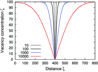
(b) 

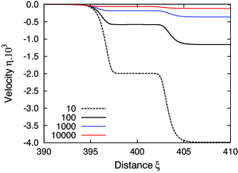
(c) 

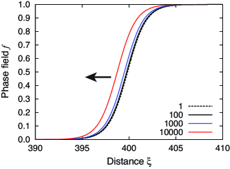
Figure 2: Dimensionless profiles of (a) vacancy concentration $\zeta$ (initial value $\zeta=100$), (b) lattice velocity $\eta$ and (c) phase field $\varphi$. The time $\tau$ is indicated in the legends. The model parameters are $\beta_{\varphi}=1$, $\beta_{s}=0.8$, $a_{\sigma}=0$ (no stress) and $a_{w}=0.5$. Note that the phase-field profile is drifting to the left (indicated by the arrow) reflecting GB migration.

Example 1. We first consider a stress-free ($a_{\sigma}=0$) bicrystal of length $\mathcal{L}=800$. The initial state is a uniform vacancy over-saturation with concentration $\zeta=100$. We impose a zero-flux condition $\partial\zeta/\partial\xi=0$ at the left end ($\mathcal{\xi}=0$) and a fixed-concentration condition $\zeta(\mathcal{L},\tau)=\zeta(\mathcal{L},0)$ at the right end. In the absence of the GB or when the latter is unable to generate/eliminate sites ($\beta_{s}=0$), this initially uniform concentration profile will not change with time. When $\beta_{s}>0$, the GB starts to eliminate excess vacancies, creating a local concentration minimum (Fig. 2). With time, this minimum deepens and widens as the vacancy concentration in the GB reaches its equilibrium value $\zeta=1$. This process is accompanied by elimination of crystal planes in the GB region resulting in shortening of both grains and thus a flow of the right grain to the left. This explains the uniform negative velocity field on the right of the GB. The GB itself also moves to the left, although slower than the right grain. Since the vacancy concentration is small, vacancies from vast lattice volumes must be absorbed to eliminate even a single lattice plane. It is not surprising, therefore, that the GB displacement is much smaller than the width of the vacancy diffusion zone around the boundary, which eventually reaches the size of the sample.

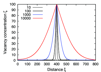
(b) 

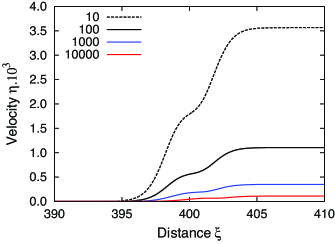
(c) 

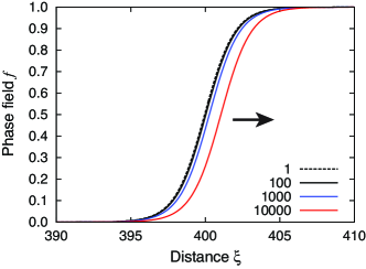
Figure 3: Dimensionless profiles of (a) vacancy concentration $\zeta$ (initial value $\zeta=1$), (b) lattice velocity $\eta$ and (c) phase field $\varphi$. The time $\tau$ is indicated in the legends. The model parameters are $\beta_{\varphi}=1$, $\beta_{s}=0.8$, $a_{\sigma}=4.6$ (tensile stress) and $a_{w}=0.5$. Note that the phase-field profile is drifting to the right (indicated by the arrow) reflecting GB migration.

Example 2. Next we consider the same bicrystal ($\mathcal{L}=800$) subject to the same boundary conditions. Suppose it has been equilibrated at zero value of the tensile stress. At a moment $\tau=0$ the stress is suddenly raised to a value $a_{\sigma}=4.6$ (tension) corresponding to the new equilibrium vacancy concentration $\zeta\approx 99.5$. To reach it, the GB generates vacancies producing a concentration maximum that grows and widens with time (Fig. 3). The vacancy generation occurs by embedding extra crystal planes on either side of the GB, which results in the motion of the right grain as well as the GB to the right. In this example, the application of the tensile stress causes the growth of both grains by accretion of material in the GB region, resulting in creep deformation of the sample. As in the previous case, the GB displacement is small in comparison with the width of the diffusion zone due to the small vacancy concentration.

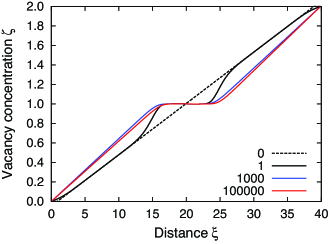
(b) 

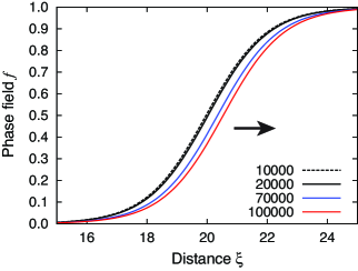
Figure 4: Dimensionless profiles of (a) vacancy concentration $\zeta$ and (b) phase field $\varphi$. The time $\tau$ is indicated in the legends. The model parameters are $\beta_{\varphi}=1$, $\beta_{s}=0.8$, $a_{\sigma}=0$ and $a_{w}=0.5$. The arrow indicates the trans-gradient induced GB migration to the right.

Example 3. Suppose the bicrystal is stress-free and a vacancy concentration gradient has been created around the initial GB position. Computationally, this has been achieved by creating a linear vacancy concentration profile increasing from $\zeta=0$ at $\mathcal{\xi}=0$ to $\zeta=2$ at $\mathcal{\xi}=\mathcal{L}$ and keeping these boundary values fixed (Fig. 4). To amplify the concentration gradient, this calculation was performed in a smaller system with $\mathcal{L}=40$. Note that in its initial position at $\xi=\mathcal{L}/2$, the GB sees the equilibrium concentration $\zeta=1$. Thus, this calculation is a test of the GB response to a vacancy concentration gradient around the equilibrium value.

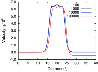
(b) 

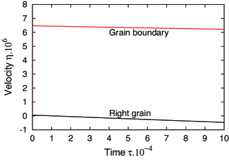
Figure 5: (a) Dimensionless profiles of the lattice velocity $\eta$ and (b) the GB velocity $\eta_{GB}$ and the velocity of the right grain as functions of time $\tau$. In (a), the time $\tau$ is indicated in the legends. The model parameters are $\beta_{\varphi}=1$, $\beta_{s}=0.8$, $a_{\sigma}=0$ and $a_{w}=0.5$.

Due to the concentration gradient, the vacancies are initially over-saturated on the right of the GB and under-saturated on the left. To approach equilibrium, excess vacancies must be eliminated by the GB on its right and generated on its left. This process is accompanied by elimination of crystal planes on the right and creation of new crystal planes on the left. As a result, locally within the GB region, the left grain grows while the right grain shrinks, causing GB migration to the right. This site generation/annihilation process results in the positive peak of the lattice velocity in the GB region (Fig. 5). The small bump near the center of the peak is a non-classical effect which originates from the deviation of the system from phase field equilibrium [the term multiplying $a_{w}$ in Eq.(134)]. The fact that the right grain has a negative velocity indicates that the net vacancy balance is slightly shifted towards annihilation. It is also observed that the height of the velocity peak decreases with time and drifts to the right together with the GB.

This example demonstrates an interesting effect in which a GB can be moved by a trans-gradient of vacancy concentration, a phenomenon which could be observable experimentally. To provide an additional proof of this effect, the calculation was repeated with the opposite sign of the vacancy concentration gradient but the same boundary values of the phase field. As expected, the gradient caused the GB to migrate to the left with a nearly identical magnitude of the velocity.

VIII Summary and conclusions

The proposed theory of creep takes classical solid-state thermodynamicsLarche73 ; Larche_Cahn_78 ; Larche1985 ; Mullins1985 as the starting point and generalizes it in at least two ways. First, we have lifted the “network constraint” and allowed lattice sites to be created or destroyed with a rate which can be a continuous function of coordinates and in addition can depend on crystallographic direction. This has been achieved by introducing two different deformation gradients co-existing in the same material, one describing local lattice distortions due to elastic strains, compositional strain and thermal expansion, and the other describing the total deformation including the permanent distortion produced by the creation and annihilation of lattice sites. The difference between the two represents the amount of creep deformation. Accordingly, its time derivative $\mathbf{R}$ defined by Eq.(49) is identified with the creep deformation rate. Similar to recent workSvoboda2006 ; Fischer2011 and by contrast to other creep theories, the creep deformation rate is a tensor that encapsulates both the volume tension and compression due to the net production or elimination of vacancies, and pure shear deformation by concurrent site generation and annihilation without altering the total number of sites.

The particular formulation of the theory presented in this paper relies on the assumption of a substitutional solid solution with a Bravais lattice. Accordingly, for a heterogeneous material its phases are assumed be “coherent” with each other, i.e., derivable from the same reference structure by affine distortions. Furthermore, our treatment of the deformation gradient $\tilde{\mathbf{F}}$ as a continuous function of coordinates implies that interfaces between the phases are coherent. In the future, this version of the theory can be generalized to solids with interstitials and non-Bravais lattices, permitting a more general treatment of the structures of the phases and inter-phase interfaces.

The tensor $\mathbf{R}$ reflects the symmetry of the material’s microstructure and the operation of particular site generation mechanisms. We gave a few examples in which some of the components of $\mathbf{R}$ are identically zero due to the absence of certain site generation mechanisms or presence of geometric restrictions. In such cases, the material can be capable of supporting static shear stresses and can reach a (constrained) thermodynamic equilibrium in a non-hydrostatic state of stress. When $\mathbf{R}=\mathbf{0}$, the theory reduces to the formulation in which the solid is subject to the “network constraint”. If all components of $\mathbf{R}$ are nonzero, the equilibrium state has to be hydrostatic. The ultimate equilibrium state of the material is uniform isotropic tension or compression.

The second generalization is the addition of phase fields and their gradients, along with gradients of concentrations of the chemical species. Owing to this non-classical character, the kinetic equations of the theory can automatically describe the evolution of microstructure as part of the creep deformation process, eliminating the need to prescribe a particular distribution of vacancy sinks and sources. For example, the site creation and annihilation can be localized in GBs by appropriate choice of the phase-field dependence of the kinetic coefficient controlling the site generation rate. If the GB moves, the vacancy sinks and sources will move together with it.

The entropy production rate derived herein identifies several dissipation mechanisms in the material: conduction of heat, diffusion of chemical species, evolution of the phase fields, viscous dissipation (e.g., by phonons), and finally site creation and annihilation. It also identifies the generalized forces and generalized fluxes corresponding to different dissipation mechanisms. It particular, the creep deformation rate $\mathbf{R}$ is identified as one such flux and the thermodynamic force driving the creep deformation is found to be $\left(\tilde{\mathbf{\boldsymbol{\sigma}}}-\omega\mathbf{I}\right)/T$, where $\omega$ is the non-classical grand potential density and $\tilde{\mathbf{\boldsymbol{\sigma}}}$ is the classical recoverable stress tensor. Diffusion is driven by gradients of the non-classical diffusion potentials $M_{i}^{*}$ and viscous dissipation by the deviation of the dynamic stress tensor $\boldsymbol{\sigma}$ from the non-classical (Korteweg) stress $(\tilde{\mathbf{\boldsymbol{\sigma}}}+\mathbf{A}^{*})$. The latter gives rise to interface stresses, which are thus automatically included in this theory.

In formulating phenomenological relations between the fluxes and forces we take into account the symmetry properties of the material.De-Groot1984 The symmetry analysis is prepared by partitioning the entropy production into groups of terms with the same tensor character. The existence or absence of coupling between different groups is established by analyzing the effect of the symmetry operations on the terms with a particular tensor character. The case of a fully isotropic material is analyzed in greatest detail. The splitting of the creep deformation rate $\mathbf{R}$ into the volume and shear components emerges as a result of this coupling analysis, with each component driven by a different thermodynamic force. The case of axial symmetry is also discussed as an example of less symmetric materials. In this case, the volume and shear components of $\mathbf{R}$ are inseparable and merge into a single tensile deformation rate $R_{n}=\mathbf{n}\cdot\mathbf{R}\cdot\mathbf{n}$, where $\mathbf{n}$ is the unit vector parallel to the axis of symmetry. Rigorous analysis of other symmetries relevant to particular classes of materials would be an interesting direction for future work.

The obtained phenomenological equations can be used for formulating a set of kinetic equations describing the evolution of the material during creep deformation. This requires input in the form of a thermodynamic equation of state, coordinate and time dependencies of the kinetic coefficients and other specific properties of the material. While this theory awaits applications to real materials, it is illustrated in this paper by a simple one-dimensional example of a bicrystal with a GB acting as a sink and source of vacancies. The kinetic equations have been formulated and solved numerically for three different cases. The calculations demonstrate how the vacancy generation or absorption due to deviations from vacancy equilibrium or caused by applied stresses can induce not only creep deformation of the sample but also GB migration (moving vacancy sink/source). The calculations also reveal an interesting effect of GB motion induced by a vacancy concentration gradient across the boundary. This trans-gradient induced GB migration might occur in processes such as radiation creep and deserves further study in the future.

Acknowledgement: We are grateful to G. B. McFadden, J. E. Guyer and J .Ovdquist for helpful discussions in the course of this research. This work was supported by the National Institute of Standards and Technology, Materials Measurement Laboratory, the Materials Science and Engineering Division.

(a) 

(a) 

(a) 

(a) 

Appendix A Exact momentum and energy balance relations

In this Appendix we derive the exact momentum and energy balance relations with respect to the lattice.

A.1 Momentum balance

Consider a fixed control region of a volume $V$. The rate of the total linear momentum $\mathbf{P}$ of the region is

$$\dfrac{d\mathbf{P}}{dt}=\intop_{V}\dfrac{\partial}{\partial t}\left(\rho\mathbf{v}\right)dV+\intop_{\partial V}\sum_{i=1}^{n}m_{i}n_{i}\mathbf{v}_{i}\left(\mathbf{v}_{i}\cdot\mathbf{n}\right)dA,$$ (138)

where the second integral represent the momentum dissipation through the boundaries. Here, $\mathbf{n}$ is a unit normal pointing outside the region and $dA$ is an increment of area of the boundary. All other notations have been defined in the main text. Applying the divergence theorem,

$$\dfrac{d\mathbf{P}}{dt}=\intop_{V}\left[\dfrac{\partial}{\partial t}\left(\rho\mathbf{v}\right)+\nabla\cdot\mathbf{Z}\right]dV,$$ (139)

where

$$\mathbf{Z}\equiv\sum_{i=1}^{n}m_{i}n_{i}\mathbf{v}_{i}\mathbf{v}_{i}=\rho\mathbf{v}_{L}\mathbf{v}_{L}+\mathbf{v}_{L}\boldsymbol{q}+\boldsymbol{q}\mathbf{v}_{L}+\mathbf{M}.$$ (140)

On the other hand, the total force acting on the region is

$$\mathbf{F}=\intop_{V}\mathbf{b}dV+\intop_{\partial V}\mathbf{n}\cdot\boldsymbol{\sigma}dA=\intop_{V}\left(\mathbf{b}+\nabla\cdot\boldsymbol{\sigma}\right)dV.$$ (141)

Writing down the Newton law $d\mathbf{P}/dt=\mathbf{F}$ we obtain the momentum balance equation in the barycentric formulation,

$$\dfrac{\partial}{\partial t}\left(\rho\mathbf{v}\right)+\nabla\cdot\mathbf{Z}=\mathbf{b}+\nabla\cdot\boldsymbol{\sigma}.$$ (142)

Using the mass conservation relation

$$\dfrac{\partial\rho}{\partial t}=-\nabla\cdot\left(\rho\mathbf{v}\right)$$ (143)

it can be shown that

$$\dfrac{\partial}{\partial t}\left(\rho\mathbf{v}\right)=\rho\dfrac{d^{L}\mathbf{v}_{L}}{dt}+\dfrac{d^{L}\boldsymbol{q}}{dt}-\nabla\cdot\left(\rho\mathbf{v}_{L}\mathbf{v}_{L}\right)-\mathbf{v}_{L}\nabla\cdot\boldsymbol{q}-\mathbf{v}_{L}\cdot\nabla\boldsymbol{q}.$$ (144)

Combining the above equations, we obtain the momentum balance equation in the lattice representation

$$\rho\dfrac{d^{L}\mathbf{v}_{L}}{dt}=\mathbf{b}+\nabla\cdot\left(\boldsymbol{\sigma}-\mathbf{M}\right)-\dfrac{d^{L}\boldsymbol{q}}{dt}-\boldsymbol{q}\nabla\cdot\mathbf{v}_{L}-\boldsymbol{q}\cdot\nabla\mathbf{v}_{L}.$$ (145)

A.2 Energy balance

The internal energy density $u$ was defined in the main text through the total energy ansatz (20). This internal energy appears in De Groot and MazurDe-Groot1984 , where it is denoted $u^{*}$, but most of their discussion is focused on an approximate internal energy defined by replacing $K$ by only the barycentric kinetic energy $\rho|\mathbf{v}|^{2}/2$. Although this approximation greatly simplifies all equations, our calculations will be based on the full kinetic energy $K$.

The energy balance is governed by the energy conservation law,

$$\dfrac{\partial e^{\prime}}{\partial t}+\nabla\cdot\left(e^{\prime}\mathbf{v}_{L}+\mathbf{J}_{u}^{L}+\mathbf{J}_{K}^{L}\right)=\dot{w},$$ (146)

where $\dot{w}$ is the rate of mechanical work per unit volume, $e^{\prime}\equiv e-\psi$ is the energy without the potential energy since the latter is already included in $\dot{w}$, $\mathbf{J}_{u}^{L}$ is the internal energy flux and $\mathbf{J}_{K}^{L}$ is the kinetic energy flux relative to the lattice. The internal energy rate

$$\dfrac{d^{L}u}{dt}+u\nabla\cdot\mathbf{v}_{L}=-\nabla\cdot\left(\mathbf{J}_{u}^{L}+\mathbf{J}_{K}^{L}\right)+\dot{w}-\left(\dfrac{d^{L}K}{dt}+K\nabla\cdot\mathbf{v}_{L}\right)$$ (147)

can be derived by computing the terms appearing in the right-hand side.

To compute $\dot{w}$, we consider a material region bounded by a set of moving markers. The total work rate on this region includes the work of volume forces and the work of stress acting on its boundary,

$$\dot{W} = \intop_{V}\sum_{i=1}^{n}n_{i}\mathbf{b}_{i}\cdot\mathbf{v}_{i}dV+\intop_{\partial V}\mathbf{n}\cdot\boldsymbol{\sigma}\cdot\mathbf{v}_{L}dA$$ (148)

$$= \intop_{V}\left[\sum_{i=1}^{n}n_{i}\mathbf{b}_{i}\cdot\mathbf{v}_{i}+\nabla\cdot\left(\boldsymbol{\sigma\cdot\mathbf{v}_{L}}\right)\right]dV,$$

from which

$$\dot{w}=\sum_{i=1}^{n}\mathbf{b}_{i}\cdot\mathbf{J}_{i}^{L}+\mathbf{v}_{L}\cdot\left(\mathbf{b}+\nabla\cdot\boldsymbol{\sigma}\right)+\boldsymbol{\sigma}:\nabla\mathbf{v}_{L}\cdot$$ (149)

The kinetic energy (21) can be split into three terms,

$$K=K_{L}+K_{d}+\boldsymbol{q}\cdot\mathbf{v}_{L},$$ (150)

where

$$K_{L}=\dfrac{1}{2}\rho|\mathbf{v}_{L}|^{2}$$ (151)

is the macroscopic kinetic energy of the lattice motion and

$$K_{d}=\sum_{i=1}^{n}\dfrac{m_{i}}{2n_{i}}\mathbf{J}_{i}^{L}\cdot\mathbf{J}_{i}^{L}=\dfrac{1}{2}\textrm{Tr}(\mathbf{M})$$ (152)

is the kinetic energy of diffusion. Calculations show that

$$\dfrac{d^{L}K_{L}}{dt}+K_{L}\nabla\cdot\mathbf{v}_{L}=\rho\dfrac{d^{L}\mathbf{v}_{L}}{dt}\cdot\mathbf{v}_{L}-\dfrac{1}{2}|\mathbf{v}_{L}|^{2}\nabla\cdot\boldsymbol{q},$$ (153)

$$\dfrac{d^{L}K_{d}}{dt}+K_{d}\nabla\cdot\mathbf{v}_{L}=-\sum_{i=1}^{n}\dfrac{m_{i}}{2n_{i}^{2}}\left(\mathbf{J}_{i}^{L}\cdot\mathbf{J}_{i}^{L}\right)\nabla\cdot\mathbf{J}_{i}^{L}+\sum_{i=1}^{n}m_{i}\mathbf{J}_{i}^{L}\cdot\dfrac{d^{L}\mathbf{w}_{i}}{dt},$$ (154)

$$\dfrac{d^{L}}{dt}\left(\boldsymbol{q}\cdot\mathbf{v}_{L}\right)+\left(\boldsymbol{q}\cdot\mathbf{v}_{L}\right)\left(\nabla\cdot\mathbf{v}_{L}\right)=\boldsymbol{q}\cdot\dfrac{d^{L}\mathbf{v}_{L}}{dt}+\mathbf{v}_{L}\cdot\dfrac{d^{L}\boldsymbol{q}}{dt}+\left(\boldsymbol{q}\cdot\mathbf{v}_{L}\right)\left(\nabla\cdot\mathbf{v}_{L}\right),$$ (155)

where we denoted $\mathbf{w}_{i}\equiv\mathbf{v}_{i}-\mathbf{v}_{L}$. Summing up Eqs.(153), (154) and (155), we obtain kinetic energy rate

$$\dfrac{d^{L}K}{dt}+K\nabla\cdot\mathbf{v}_{L} = \left(\rho\mathbf{v}_{L}+\boldsymbol{q}\right)\cdot\dfrac{d^{L}\mathbf{v}_{L}}{dt}+\mathbf{v}_{L}\cdot\dfrac{d^{L}\boldsymbol{q}}{dt}+\left(\boldsymbol{q}\cdot\mathbf{v}_{L}\right)\left(\nabla\cdot\mathbf{v}_{L}\right)-\dfrac{1}{2}|\mathbf{v}_{L}|^{2}\nabla\cdot\boldsymbol{q}$$ (156)

$$-\sum_{i=1}^{n}\dfrac{m_{i}}{2n_{i}^{2}}\left(\mathbf{J}_{i}^{L}\cdot\mathbf{J}_{i}^{L}\right)\nabla\cdot\mathbf{J}_{i}^{L}+\sum_{i=1}^{n}\dfrac{m_{i}}{n_{i}}\mathbf{J}_{i}^{L}\cdot\dfrac{d^{L}\mathbf{w}_{i}}{dt}.$$

For the lattice flux of kinetic energy we have

$$\mathbf{J}_{K}^{L} = \sum_{i=1}^{n}\dfrac{1}{2}m_{i}n_{i}\left(\mathbf{v}_{i}\cdot\mathbf{v}_{i}\right)\left(\mathbf{v}_{i}-\mathbf{v}_{L}\right)$$ (157)

$$= \sum_{i=1}^{n}\dfrac{m_{i}}{2n_{i}^{2}}\left(\mathbf{J}_{i}^{L}\cdot\mathbf{J}_{i}^{L}\right)\mathbf{J}_{i}^{L}+\dfrac{1}{2}\boldsymbol{q}|\mathbf{v}_{L}|^{2}+\mathbf{M}\cdot\mathbf{v}_{L}.$$

Inserting Eqs.(149), (156) and (157) in the right-hand side of Eq.(147), after lengthy calculations we finally obtain

$$\dfrac{d^{L}u}{dt}+u\nabla\cdot\mathbf{v}_{L} = -\nabla\cdot\mathbf{J}_{u}^{L}+\sum_{i=1}^{n}\mathbf{b}_{i}\cdot\mathbf{J}_{i}^{L}+\left(\boldsymbol{\sigma}-\mathbf{M}\right):\nabla\mathbf{v}_{L}$$ (158)

$$-\sum_{i=1}^{n}\left\{\nabla\left[\dfrac{m_{i}}{2n_{i}^{2}}\left(\mathbf{J}_{i}^{L}\cdot\mathbf{J}_{i}^{L}\right)\right]+m_{i}\dfrac{d^{L}\mathbf{v}_{i}}{dt}\right\}\cdot\mathbf{J}_{i}^{L}.$$

Appendix B Justification of the approximate form of the entropy production

In the main text, we derived the exact expression for the entropy production rate (72). Deriving the linear constitutive relations we assumed that the fluxes and forces were both small. Under this linear approximation, all terms quadratic in fluxes and/or forces must be neglected. Tensor $\mathbf{M}$ defined by Eq.(18) is quadratic in the diffusion fluxes $\mathbf{J}_{i}^{L}$ and can be neglected. Further, the term $m_{i}(\mathbf{J}_{i}\cdot\mathbf{J}_{i})/2n_{i}^{2}$ in the driving force of diffusion is also quadratic in diffusion fluxes and can also be neglected.

Furthermore, for slow processes such as creep the inertia terms $m_{i}d^{L}\mathbf{v}_{i}/dt$ can be neglected after a short transient. To demonstrate this, consider an isotropic materials not subject to external fields. Assuming a uniform temperature field, diffusion is decoupled from all other processes and is described by the equations

$$\mathbf{J}_{i}^{L}=-\dfrac{1}{T}\sum_{j=1}^{n}L_{ij}\left(\nabla M_{j}^{*}+m_{j}\dfrac{d^{L}\mathbf{v}_{j}}{dt}\right),\enskip\enskip i=1,...,n$$ (159)

where the $n\times n$ matrix of kinetic coefficients $\mathbf{L}$ is symmetric and positive definite.

Rewrite (159)

$$\mathbf{J}_{i}^{L}=-\dfrac{1}{T}\sum_{j=1}^{n}L_{ij}\left(\nabla M_{j}^{*}+m_{j}\dfrac{d^{L}\mathbf{w}_{j}}{dt}+m_{j}\dfrac{d^{L}\mathbf{v}_{L}}{dt}\right),\enskip\enskip i=1,...,n$$ (160)

and consider the effect of each inertia term separately. To understand the role of the first inertia term, suppose all other driving forces are zero. Neglecting also the cross-effects among the diffusion fluxes, the diffusion equations reduce to

$$\mathbf{w}_{i}=-\dfrac{m_{i}L_{ii}}{Tn_{i}}\dfrac{d^{L}\mathbf{w}_{i}}{dt}\equiv-\tau_{i}\dfrac{d^{L}\mathbf{w}_{i}}{dt},\enskip\enskip i=1,...,n.$$ (161)

Assuming that

$$\tau_{i}=\dfrac{m_{i}L_{ii}}{Tn_{i}}$$ (162)

is a slow-varying function of time, Eqs.(161) have approximately exponential solutions $\mathbf{w}_{i}\propto\exp(-t/\tau_{i})$ showing that any initial acceleration of the particles relative to the lattice damps after a characteristic time $\tau_{i}$. Thus, for processes occurring on time scales much longer than $\tau_{i}$, the inertia terms $m_{j}d^{L}\mathbf{w}_{j}/dt$ can be neglected.

To evaluate typical values of $\tau$, take one of the species, say 1, and express the kinetic coefficient $L_{11}$ through the diffusion coefficient $D_{1}$ via $L_{11}=n_{1}D_{1}/k_{B}$, which gives $\tau=m_{1}D_{1}/(k_{B}T)$. Taking the molecular weight of 100 a.m.u., the upper bound of the diffusion coefficients in solids $D_{1}=10^{-9}$ m²/s and the temperature of 1000 K we obtain $\tau\approx 10^{-14}$ s. At lower temperatures $\tau$ is even smaller. Thus the time scale of damping of the inertia terms is much smaller than the typical time scale of creep tests (many hours).

The inertia terms $m_{i}d^{L}\mathbf{v}_{L}/dt$ originate from the accelerated lattice motion due to applied mechanical stress as well as the site generation and other relatively slow processes. Before the material reaches mechanical equilibrium, the lattice velocities can be very high, possibly comparable with the speed of sound, and the inertia force $m_{i}d^{L}\mathbf{v}_{L}/dt$ can be significant. But the subsequent creep deformation is a slow process in which the material maintains mechanical equilibrium and $d^{L}\mathbf{v}_{L}/dt$ reflects only the slow changes in the creep deformation rate. As a crude estimate, the magnitude of the lattice acceleration is related to variations in the creep deformation $\dot{\epsilon}$ by

$$\dfrac{d^{L}\ln|\mathbf{v}_{L}|}{dt}\approx\dfrac{d\ln\dot{\epsilon}}{dt}.$$ (163)

During the steady-state creep, $\dot{\epsilon}$ remains nearly constant and depends only on the applied stress and temperature, so that the inertia terms $m_{i}d^{L}\mathbf{v}_{L}/dt$ can be neglected. During the primary and tertiary stages, the right-hand side of Eq.(163) still remains small. For example, typical steady-state creep rates in metallic alloys are $\dot{\epsilon}\approx 10^{-6}$ to $10^{-3}$ s^-1. During the primary and tertiary stages, the rate changes by at most an order of magnitude over hundreds of hours. Thus, as an upper bound $\ddot{\epsilon}\approx 10^{-7}$ s^-2 and thus $d^{L}\ln|\mathbf{v}_{L}|/dt\approx 0.1$ s^-1.

To show that the inertia effects are negligible, we combine the particle conservation law with the diffusion equation for species $i$,

$$\mathbf{J}_{i}^{L}=-\dfrac{1}{T}L_{ii}\left(\nabla M_{j}^{*}+m_{i}\dfrac{d^{L}\mathbf{v}_{L}}{dt}\right),$$ (164)

in which we again neglected the cross effects among the fluxes. Treating the kinetic coefficient as a constant,

$$\dfrac{\partial n_{i}}{\partial t}=-\dfrac{1}{T}L_{ii}\nabla^{2}M_{j}^{*}-\nabla\cdot\left(n_{i}\mathbf{v}_{L}-\dfrac{1}{T}L_{ii}m_{i}\dfrac{d^{L}\mathbf{v}_{L}}{dt}\right).$$ (165)

The ratio of the second term to the first inside the divergence is on the order of

$$\dfrac{L_{ii}m_{i}}{Tn_{i}}\dfrac{d^{L}\ln|\mathbf{v}_{L}|}{dt}=\tau_{i}\dfrac{d^{L}\ln|\mathbf{v}_{L}|}{dt},$$ (166)

where $\tau_{i}$ is the characteristic time (162). The latter was estimated to be $\sim 10^{-14}$ s. Thus, the inertia term in Eq.(165) is more than ten orders of magnitude smaller than the normal term $n_{i}\mathbf{v}_{L}$, reducing the diffusion equation to the usual form

$$\dfrac{\partial n_{i}}{\partial t}=-\dfrac{1}{T}L_{ii}\nabla^{2}M_{j}^{*}-\nabla\cdot\left(n_{i}\mathbf{v}_{L}\right).$$ (167)

These estimates justify the approximate form (73) of the entropy production for creep applications.

References

- (1) G. B. Stephenson, Acta Metall. Mater. 36, 2663 (1988).
- (2) F. R. Nabarro, Deformation of crystals by the motion of single ions, in Report of a Conference on Strength of Solids, pages 75–90, London, UK, 1948, The Physical Society.
- (3) C. J. Herring, J. Appl. Phys. 21, 437 (1950).
- (4) R. L. Coble, J. Appl. Phys. 34, 1679 (1963).
- (5) F. A. Mohamed and Y. Li, Mater. Sci. Eng. A 298, 1 (2001).
- (6) S. R. De Groot and P. Mazur, Non-equilibrium thermodynamics, Dover, New York, 1984.
- (7) J. Svoboda, F. D. Fischer, and P. Fratzl, Acta Mater. 54, 3043 (2006).
- (8) F. D. Fischer and J. Svoboda, Int. J. Plast. 27, 1384 (2011).
- (9) R. F. Sekerka and J. W. Cahn, Acta Mater. 52, 1663 (2004).
- (10) F. Larché and J. W. Cahn, Acta Metall. 21, 1051 (1973).
- (11) F. C. Larché and J. W. Cahn, Acta Metall. 26, 1579 (1978).
- (12) F. C. Larché and J. W. Cahn, Acta Metall. 33, 331 (1985).
- (13) W. W. Mullins and R. F. Sekerka, J. Chem. Phys. 82, 5192 (1985).
- (14) P. W. Voorhees and W. C. Johnson, The thermodynamics of elastically stresses crystals, in Solid State Physics, edited by H. Ehrenreich and F. Spaepen, volume 59, pages 2–201, Elsevier Academic Press, 2004.
- (15) T. Frolov and Y. Mishin, Phys. Rev. B 82, 174113 (2010).
- (16) J. W. Gibbs, The collected works of J. W. Gibbs, volume 1, Yale University Press, New Haven, 1948.
- (17) F. Bloch, Z. Phys. 74, 295 (1932).
- (18) V. L. Ginzburg and L. D. Landau, Zh. Eksp. Teor. Fiz. 20, 1064 (1950).
- (19) J. W. Cahn and J. E. Hilliard, J. Chem. Phys. 28, 258 (1958).
- (20) R. F. Sekerka, Philos. Mag. 91, 3 (2011).
- (21) N. Zhou, C. Shen, M. Mills, and Y. Wang, Phil. Mag. 90, 405 (2010).
- (22) J. Philibert, Atom Movements – Diffusion and Mass Transport in Solids, Les Editions de Physique, Les Ulis, 1991.
- (23) L. E. Malvern, Introduction To The Mechanics Of A Continuous Medium, Prentice-Hall, Upper Saddle River, 1969.
- (24) B. A. Bilby, Continuous distributions of dislocations, in Progress in Solid Mechanics, edited by I. N. Sneddon and R. P. Hill, volume 1, chapter 7, pages 330–398, 1960.
- (25) R. O. Simmons and R. W. Balluffii, Phys. Rev. 117, 52 (1960).
- (26) R. O. Simmons and R. W. Balluffii, Phys. Rev. 119, 600 (1960).
- (27) I. M. Gelfand and S. V. Fomin, Calculus of variations, Prentice-Hall, Englewood Cliffs, NJ, 1964.
- (28) D. J. Korteweg, Arch. Nèerl. Sci. Exactes Nat., Ser. II 6, 1 (1901).
- (29) L. Onsager, Phys. Rev. 37, 405 (1931).
- (30) L. Onsager, Phys. Rev. 38, 2265 (1931).
- (31) J. F. Nye, Physical Properties of Crystals, Clarendon Press, Oxford, 1985.
- (32) C. Rottman, Phys. Rev. B 38, 12031 (1988).
- (33) W. C. Johnson, Acta Mater. 48, 433 (2000).
- (34) V. I. Levitas, Phys. Rev. B 87, 054112 (2013).
- (35) C. Herring, in The Physics of Powder Metallurgy, edited by R. Gomer and C. S. Smith, McGraw-Hill, New York, 1949.
(a)
(b)
(c)
(a)
(b)
(c)
(a)
(b)
(a)
(b)