Linear magnetoconductivity in multiband spin-density-wave metals with nonideal nesting

Abstract

In several parent iron-pnictide compounds the resistivity has an extended range of linear magnetic field dependence. We argue that there is a simple and natural explanation of this behavior. Spin density wave transition leads to Fermi-surface reconstruction corresponding to strong modification of the electronic spectrum near the nesting points. It is difficult for quasiparticles to pass through these points during their orbital motion in magnetic field, because they must turn sharply. As the area of the Fermi surface affected by the nesting points increases proportionally to magnetic field, this mechanism leads to the linear magnetoresistance. The crossover between the quadratic and linear regimes takes place at the field scale set by the SDW gap and scattering rate.

The studying of transport in magnetic field is the simplest way to characterize electronic structure of new materials and quasiparticle scattering. The transport properties of the recently discovered iron pnictides in magnetic field have some anomalous features. In particular, the resistivity is found to have linear dependence on magnetic field for several parent and underdoped compounds with spin-density wave (SDW) long-range order, such as CaFe₂As₂Torikachvili et al. (2009), BaFe₂As₂ Ishida et al. (2011), Ba(Fe_1-xRu_xAs)₂Tanabe et al. (2011), PrFeAsO Bhoi et al. (2011).

The linear magnetoresistance is not a new effect. It was first reported by Kapitza for bismuth in 1928 Kapitza (1928), see also Yang et al. (1999), and later was found in several other metals, see, e.g., Refs. Simpson, 1973; Xu et al., 1997; Bud’ko et al., 1998; Lee et al., 2002; Wang and Petrovic, 2012 and discussion in the Pippard book Pippard (1989). One can hardly expect a single universal mechanism of this phenomenon. In different materials the linear magnetoresistance may appear due to completely different reasons. In particular, Abrikosov demonstrated that the linear dependence appears in the case of Dirac electronic spectrum Abrikosov (1998); *AbrikosovPhysRevB99. This mechanism is frequently used for interpretation of the iron-pnictides data. Moreover, the linear magnetoresistance sometimes is presented as a proof for the Dirac spectrum.

We argue in this letter that the presence of the SDW order leads to a simple and natural mechanism for the linear magnetoresistance in the parent iron-pnictide compounds, which, surprisingly, was not discussed. The SDW order mixes the electron and hole bands which have different shapes. As a consequence, the nesting at the SDW wave vector is only ideal at lines on the Fermi surface. Weak SDW order only modifies electronic spectrum near these lines leading to reconstruction of the Fermi surface, as illustrated in Fig. 1. For fixed $p_{z}$ cross section the Fermi surface consists of four banana-shape pockets (only halves of two bananas are shown in Fig. 1). Every pocket is characterized by two sharp turning regions (banana tips) located near the nesting points. In the magnetic field applied along $z$ direction the quasiparticles move along the orbits located in the $xy$ plane. The turning regions where the orbits transfer in between the electron and hole branches the velocity changes sharply and smooth orbital motion is interrupted. This leads to enhanced quadratic magnetoconductivity at small magnetic field and extended region of the linear magnetoconductivity. The latter effect appears due to the linear growth with the field of regular regions of Fermi surface affected by the turning regions. The crossover field between the two regimes is proportional to the SDW gap $\Delta_{m}$ and inversely proportional to the scattering time $\tau$. In the quadratic regime at small fields the turning-point contribution exceeds the conventional magnetoconductivity $\Delta\sigma(H)/\sigma(0)\sim(eH\tau/mc)^{2}$ by the factor $\sim\varepsilon_{F}/\Delta_{m}$, where $m$ is the effective mass and $\varepsilon_{F}$ is the Fermi energy. This mechanism has been considered in Ref. Fenton and Schofield, 2005 for a metal with a single circular Fermi surface reconstructed by commensurate density wave.

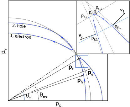
Figure 1: Fermi surface in the region $p_{x},p_{y}>0$ for a two-band metal with the SDW long-range order. Dashed lines show the bare Fermi surfaces. The electron Fermi surface is displaced by the ordering wave vector $\mathbf{Q}$ to zone center. Arrows show direction of the orbital motion in the magnetic field. The inset zooms into the region near one turning point.

The Fermi surface reconstruction caused by the magnetic transition in real materials has been explored by ARPESKondo et al. (2010); *FuglsangJensenPhysRevB11; *YiNewJP12 and quantum oscillationsTerashima et al. (2011). It may be rather complicated. To illustrate the mechanism, we consider a simple two-band model with the SDW order, see, e.g., Ref. Vorontsov et al., 2010, which also has been used to describe the SDW transition in chromium Rice (1970). The model is described by the Hamiltonian

$$\mathcal{H}=\mathcal{H}_{0}+\mathcal{H}_{AF},$$ (1)

where the free-electron part is composed of the electron and hole contributions

$$\mathcal{H}_{0}=\sum_{\mathbf{p},\sigma}\left(\xi_{1,\mathbf{p}}c_{\mathbf{p}\sigma}^{\dagger}c_{\mathbf{p}\sigma}+\xi_{2,\mathbf{p}}d_{\mathbf{p}\sigma}^{\dagger}d_{\mathbf{p}\sigma}\right)$$ (2)

and the antiferromagnetic part is given by

$$\mathcal{H}_{AF}=-\sum_{\mathbf{p},\sigma}\sigma\Delta_{m}(c_{\mathbf{p}\sigma}^{\dagger}d_{\mathbf{p}\sigma}+d_{\mathbf{p}\sigma}^{\dagger}c_{\mathbf{p}\sigma})$$ (3)

with $\Delta_{m}$ being the SDW gap.

The simplest shapes of the free-electron spectra qualitatively describing iron pnictides are parabolic bands,

$$\xi_{1,\mathbf{p}}=\varepsilon_{1,0}-\mu+\frac{p_{x}^{2}}{2m_{x}}+\frac{p_{y}^{2}}{2m_{y}},\ \xi_{2,\mathbf{p}}=\varepsilon_{2,0}-\mu-\frac{p^{2}}{2m}.$$

These bands are characterized by the Fermi momenta,

$$p_{F,j}=\sqrt{2m_{j}\left(\mu-\varepsilon_{1,0}\right)},\ p_{F,h}\equiv p_{F,2}=\sqrt{2m\left(\varepsilon_{2,0}-\mu\right)}$$

with $j=x,y$. The angular-dependent Fermi momentum for the electronic band is given by $p_{F,1}(\theta)=\left(\cos^{2}\theta/p_{F,x}^{2}+\sin^{2}\theta/p_{F,y}^{2}\right)^{-1/2}$. In the further analysis, we assume that for the selected $p_{z}$ cross section the inequality $p_{F,x}>p_{F,h}>p_{F,y}$ holds. Introducing ratios, $r_{\alpha}=p_{F,h}/p_{F,\alpha}$ with $r_{x}<1$ and $r_{y}>1$, we obtain that the ideal nesting is realized at the angles satisfying

$$\tan\theta_{\mathrm{ns}}=\sqrt{\frac{1-r_{x}^{2}}{r_{y}^{2}-1}}.$$

These nesting angles depend on the z-axis momentum $p_{z}$ and trace the nesting lines on the Fermi surface. To proceed, we will analyze the electronic spectrum near the nesting angles in the presence of the SDW order.

In the SDW state the quasiparticle spectrum has the following form Bazaliy et al. (2004); Lin and Millis (2005); Vorontsov et al. (2010)

$$E_{\mathbf{p},\pm}=\frac{\xi_{+}}{2}\pm\sqrt{\frac{\xi_{-}^{2}}{4}+\Delta_{m}^{2}}$$ (4)

with $\xi_{\pm}=\xi_{1,\mathbf{p}}\pm\xi_{2,\mathbf{p}}$. We assume $\Delta_{m}\ll\max_{FS}|\xi_{-}|$ so that the SDW order only modifies the spectrum near the nesting angles. For the branches crossing the Fermi level the sign has to be selected as $\pm\rightarrow\mathrm{sgn}(p_{F,1}-p_{F,2})$. The Fermi velocities for the modified spectrum are

$$\mathbf{v}=\frac{\mathbf{v}_{+}}{2}\pm\frac{\mathbf{v}_{-}}{2}\frac{\xi_{-}}{\sqrt{\xi_{-}^{2}+4\Delta_{m}^{2}}}$$ (5)

with $\mathbf{v}_{\pm}=\mathbf{v}_{1}\pm\mathbf{v}_{2}$ and $\mathbf{v}_{\alpha}=\partial\xi_{\alpha,\mathbf{p}}/\partial\mathbf{p}$. It is convenient to use the polar coordinates $(p_{x},p_{y})=(p\cos\theta,p\sin\theta)$ for fixed $p_{z}$ and introduce the radial and angular components of the Fermi velocity, $v_{\alpha,p}=\frac{d\xi_{\alpha,\mathbf{p}}}{dp}$, $v_{\alpha,\theta}=\frac{1}{p}\frac{d\xi_{\alpha,\mathbf{p}}}{d\theta}$ where $\alpha$ is the band index. As the second band is assumed to have the holelike spectrum, we have $v_{2,p}<0$.

In the case of weak SDW order, using linear expansion near the Fermi momenta $\xi_{\alpha,\mathbf{p}}\approx v_{\alpha,p}(p-p_{F,\alpha})$, we obtain from $E_{\mathbf{p},\pm}\!=0$ the renormalized Fermi surface

$$p_{F,\pm}\approx\frac{p_{F,1}\!+\!p_{F,2}}{2}\pm\sqrt{\frac{\left(p_{F,1}\!-\!p_{F,2}\right)^{2}}{4}-\frac{\Delta_{m}^{2}}{v_{1,p}|v_{2,p}|}}$$

(we omitted $\theta$ dependence in all $p_{F}$’s). It consists of four banana-shaped sections, the two banana halves are shown in Fig. 1. Each section has two sharp turning points (tips of banana). The angles of these turning points, $\theta_{t}$, can be found from the following condition

$$\left|p_{F,1}(\theta_{t})-p_{F,2}(\theta_{t})\right|\approx\frac{2\Delta_{m}}{\sqrt{v_{1,p}|v_{2,p}|}}$$ (6)

and the Fermi momentum at the turning point is $p_{t}=\left(p_{t,1}+p_{t,2}\right)/2$ with $p_{t,\alpha}=p_{F,\alpha}(\theta_{t})$. The Fermi surface is eliminated in the angular range

$$|\theta-\theta_{ns}|<|\theta_{t}-\theta_{ns}|\approx\frac{2\sqrt{v_{1,p}|v_{2,p}|}\Delta_{m}}{\left[\mathbf{v}_{1}\times\mathbf{v}_{2}\right]_{z}p_{t}}.$$

As the curvature of the Fermi surface sharply increases near the turning points, they have strong influence on transport properties at small magnetic fields.

Within the relaxation-time approximation for the Boltzmann equation, the classical conductivity tensor for arbitrary magnetic field is given by

$$\sigma_{\alpha\beta}=2e^{2}\sum_{\mathrm{bands}}\int\frac{dp_{z}}{(2\pi)^{3}}S_{\alpha\beta}(p_{z}),$$ (7)

where $S_{\alpha\beta}(p_{z})$ describes the contribution from a single $p_{z}$ slice

$$S_{\alpha\beta}\!=\!\frac{c}{eH}\int\frac{dp}{v}v_{\beta}\!\int_{p}\frac{dp^{\prime}}{v^{\prime}}v_{\alpha}^{\prime}\exp\left(\!-\!\int_{p}^{p^{\prime}}\frac{dp^{\prime\prime}}{v^{\prime\prime}}\frac{c}{eH\tau}\right).$$ (8)

All $p$ integrals are performed along the fixed-$p_{z}$ orbits on the Fermi surface. This presentation is similar to the so-called Shockley “tube integral”Shockley (1950); Abdel-Jawad et al. (2006). It goes beyond the small-field expansion and provides a very convenient basis for analysis of the conductivity especially when either the scattering rate $1/\tau$ or the Fermi velocity $v$ have sharp features.

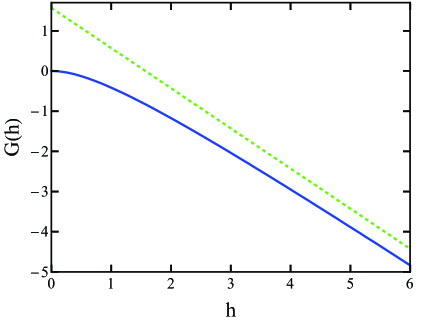
Figure 2: Function $G(h)$ in Eq. (12) which determines shape of magnetoconductivity. Dashed line shows the high-field asymptotics.

We assume that the scattering rate is regular near the turning point and the anomalous behavior only appears due to modification of spectrum. This assumption definitely breaks down in the vicinity of the SDW transition point $T_{m}$ where scattering on the magnetic fluctuations becomes strong. The integral in the exponent of Eq. (8) describes the orbital motion of the quasiparticles along the Fermi surface in the magnetic field. The SDW coupling forces the carriers to switch between the hole and electron orbits in the vicinity of the turning regions.

The simplest approximation is to treat the turning region as a point where the Fermi surface has a sharp cusp and the velocity jumps. This approximation actually gives correct result at high magnetic fields. We consider the contribution from the small section of the Fermi surface near the turning point in which the orbital motion starts at the point $\mathbf{p}_{h}$ of the hole branch and ends at the point $\mathbf{p}_{e}$ of the electron branch (this sets the limits for the $p$ integral in Eq. (8)). The distances from these points to $\mathbf{p}_{t}=(p_{t,x},p_{t,y})$ are in the intermediate range: they are much smaller than the Fermi momentum but the SDW corrections to the spectrum are assumed already to be small. The former assumption allows us to neglect in this region the bare curvature of the Fermi surface. In this case the direct calculation of the contribution from one turning point gives $S_{xx}\!\approx\tau v_{x,2}^{2}\frac{\left|\mathbf{p}_{t}-\mathbf{p}_{h}\right|}{v_{2}}+\tau v_{x,1}^{2}\frac{\left|\mathbf{p}_{e}-\mathbf{p}_{t}\right|}{v_{1}}+v_{x,2}\left(v_{x,1}\!-\!v_{x,2}\right)\frac{eH\tau^{2}}{c}$. For the symmetric point $(-p_{t,x},p_{t,y})$ the orbital motion starts at the electronic branch and ends at the hole branch. Therefore the contribution from this point to the field dependent part is $S_{xx}(H)\!-\!S_{xx}(0)\!\approx\!v_{1,x}\left(v_{2,x}\!-\!v_{1,x}\right)eH\tau^{2}/c$. Collecting contributions from the all eight turning points, we obtain.

$$S_{xx}^{(\mathrm{tp})}(H)-S_{xx}(0)\approx-4\left(v_{2,x}-v_{1,x}\right)^{2}\frac{eH\tau^{2}}{c}$$ (9)

We see that treating the turning regions as sharp cusps leads to linear magnetoconductivity. As can be seen from Eq. (8), this dependence appears because the Fermi momentum range within which quasiparticle can cross the turning point during its orbital motion is proportional to the magnetic field, $\Delta p=veH\tau/c$.

An accurate consideration should take into account a finite curvature of the Fermi surface in the turning region. To perform $p$-integrals over the Fermi surface, we have to find good parametrization. Due to the very simple dependence of velocity on the parameter $\xi_{-}$, Eq. (5), it is convenient to parametrize the integration over the Fermi surface in terms of this parameter. For small shift of $\mathbf{p}$ along the Fermi surface perpendicular to $z$ direction we have $d\mathbf{p}=\frac{dp}{v}\mathbf{v}\times\mathbf{n}_{z}$. As $d\xi_{-}=\mathbf{v}_{-}d\mathbf{p}$, using Eq. (5) for velocity, we straightforwardly derive the relation

$$\frac{dp}{v}=\frac{d\xi_{-}}{\left[\mathbf{v}_{1}\times\mathbf{v}_{2}\right]_{z}},$$

which we can use to perform the integration over the Fermi surface in Eq. (8). In the vicinity of the nesting point we can neglect variations of $\left[\mathbf{v}_{1}\times\mathbf{v}_{2}\right]_{z}$. Introducing the new variable

$$w=\frac{c}{eH\tau}\frac{\xi_{-}}{\left[\mathbf{v}_{1}\times\mathbf{v}_{2}\right]_{z}}$$

and the reduced field $h=H/H_{\Delta}$ with the field scale

$$H_{\Delta}=\frac{2c\Delta_{m}}{e\tau\left[\mathbf{v}_{1}\times\mathbf{v}_{2}\right]_{z}},$$ (10)

we obtain $\xi_{-}/2\Delta_{m}=hw$ and

$$\mathbf{v}(w)=\frac{\mathbf{v}_{+}}{2}\pm\frac{\mathbf{v}_{-}}{2}\frac{hw}{\sqrt{h^{2}w^{2}+1}}.$$

As a result, we obtain $S_{\alpha\beta}$ in Eq. (8) in convenient for calculation form

$$S_{\alpha\beta}=\frac{eH\tau^{2}}{c}\int dwv_{\beta}(w)\int_{w}dw_{1}v_{\alpha}(w_{1})\exp\left[-\left(w_{1}-w\right)\right].$$

We consider the $E_{\mathbf{p},+}$ branch located at $\theta<\theta_{t}$ which is shown in the inset of Fig. 1. For this branch the velocity changes from the bare hole velocity $\mathbf{v}_{2,x}$ to the bare electron velocity $\mathbf{v}_{1,x}$ as $w$ changes from large negative to large positive values.

The contribution to the conductivity from one turning point in the $p_{z}$ slice,

$$S_{xx}(H)=\frac{2\tau\Delta_{m}h}{\left[\mathbf{v}_{1}\times\mathbf{v}_{2}\right]_{z}}\int_{w_{h}}^{w_{e}}dw\int_{w}dw_{1}\exp\left[-\left(w_{1}\!-\!w\right)\right]$$

$$\times\!\left(\frac{v_{+,x}}{2}\!+\!\frac{v_{-,x}}{2}\frac{hw}{\sqrt{h^{2}w^{2}\!+\!1}}\right)\left(\frac{v_{+,x}}{2}\!+\!\frac{v_{-,x}}{2}\frac{hw_{1}}{\sqrt{h^{2}w_{1}^{2}\!+\!1}}\right).$$

While the whole Fermi surface additively contributes to the zero-field conductivity, the finite magnetoconductivity only appears due to the finite Fermi surface curvature. As the turning regions have the largest curvature, they dominate in the magnetoconductivity. The total contribution from all eight turning points to the field-induced change of $S_{xx}$ can be represented as

$$S_{xx}^{(\mathrm{tp})}(H)-S_{xx}(0)=\frac{8v_{-,x}^{2}\tau\Delta_{m}}{\left[\mathbf{v}_{1}\times\mathbf{v}_{2}\right]_{z}}G(h),$$ (11)

$$G(h)=\int_{0}^{\infty}dx\int_{0}^{\infty}dy\exp\left(-y\right)$$

$$\times\left(\frac{x^{2}-h^{2}y^{2}/4}{\sqrt{\left(x+h\frac{y}{2}\right)^{2}\!+1}\sqrt{\left(x-h\frac{y}{2}\right)^{2}\!+1}}-\frac{x^{2}}{x^{2}\!+1}\right).$$ (12)

The dimensionless function $G(h)$ is plotted in Fig. 2 and has the following asymptotics

$$G(h)=\genfrac{\{}{.}{0.0pt}{}{-\frac{3\pi}{16}h^{2}\text{ for }h\ll 1}{\frac{\pi}{2}-h\text{ for }h\gg 1}.$$

The linear asympotics reproduces the result (9) obtained by direct calculation. The typical field scale describing the crossover between these two regimes is given by Eq. (10).Fenton and Schofield (2005) It is proportional to the SDW gap and inversely proportional to the scattering time.

Using presentation for the zero-field conductivity $\sigma_{xx}(0)=2e^{2}\sum_{\mathrm{bands}}\int\frac{dp_{z}d\theta}{(2\pi)^{3}}m(\theta)v_{x}^{2}(\theta)\tau(\theta)$, where $m(\theta)$ is the cyclotronic mass defined for the bare bands, we can present the relative change of conductivity due to the turning points at small fields, $H\ll H_{\Delta}$, as

$$\frac{\sigma_{xx}^{(\mathrm{tp})}(H)-\sigma_{xx}(0)}{\sigma_{xx}(0)}=-\frac{3}{32}\left(\frac{eH\tau}{c}\right)^{2}\frac{\left\langle v_{-,x}^{2}\left[\mathbf{v}_{1}\times\mathbf{v}_{2}\right]_{z}\right\rangle}{\left\langle mv_{x}^{2}\right\rangle\Delta_{m}}.$$ (13)

Since the conventional magnetoconductivity can be estimated as $\left[\sigma_{xx}^{(0)}(H)\!-\!\sigma_{xx}(0)\right]/\sigma_{xx}(0)\!\approx\!-\left[eH\tau/(mc)\right]^{2}$, we can see that the contribution from the turning points exceeds the conventional one by the factor $\varepsilon_{F}/\Delta_{m}$. In the linear regime, for $H\gg H_{\Delta}$, the relative change of conductivity can be evaluated as

$$\frac{\sigma_{xx}^{(\mathrm{tp})}(H)\!-\!\sigma_{xx}(0)}{\sigma_{xx}(0)}\!=\!\frac{\left\langle\frac{v_{-,x}^{2}}{\left[\mathbf{v}_{1}\times\mathbf{v}_{2}\right]_{z}}\right\rangle}{\left\langle|m|v_{x}^{2}\right\rangle}\Delta_{m}\!-\frac{\left\langle v_{-,x}^{2}\right\rangle}{\pi\left\langle|m|v_{x}^{2}\right\rangle}\frac{\tau eH}{c}$$ (14)

We emphasize that the linear term does not depend on the SDW gap and coexists with the smaller quadratic contribution coming from the regular Fermi-surface. The linear behavior holds until $eH\tau/(mc)\ll 1.$

In conclusion, we considered magnetoconductivity for a multiband metal with the SDW order. We demonstrated that, due to appearance of sharp turning points at the Fermi surface, magnetoconductivity becomes linear when the magnetic field exceeds the field scale proportional to the SDW gap and inversely proportional to the scattering time. This mechanism provides a more natural explanation for the linear magnetoresistance observed in iron pnictides Torikachvili et al. (2009); Ishida et al. (2011); Tanabe et al. (2011); Bhoi et al. (2011) than the popular mechanism based on Dirac spectrum. Taking typical values $v=10^{7}$cm/sec, $\Delta_{m}=10$ meV, and $\tau=10^{-12}$ sec, we estimate $H_{\Delta}\approx 2$T, in qualitative agreement with experiment. As both $\Delta_{m}$ and $\tau$ increase with decreasing temperature, we can expect nonmonotonic temperature dependence of the field scale. Namely, we can expect sharpening of the magnetic field dependence as the temperature approaches the transition point due to decrease of $\Delta_{m}$ and at low temperatures due to increase of $\tau$. Such behavior was not observed. Typically, the field scale monotonically decreases with temperature Ishida et al. (2011); Tanabe et al. (2011), as expected when the temperature dependence of $\tau$ dominates. However, no detailed study of magnetoresistance in the close vicinity of the SDW transition was reported so far.

The localized Fermi surface reconstruction is not the only mechanism which can lead to the linear magnetoconductivity. Alternatively, close to the transition point the scattering caused by the antiferromagnetic fluctuations leads to suppression of the relaxation time near the nesting points (“hot spots”). This also gives the linear magnetoconductivity due to the interruption of the orbital motion Rosch (2000). The scattering mechanism clearly becomes dominant as the temperature approaches $T_{m}$. The crossover between the two mechanisms in the vicinity of the transition point is an interesting topic for future study.

I would like to thank Vivek Mishra for useful discussions. This work was supported by UChicago Argonne, LLC, operator of Argonne National Laboratory, a U.S. Department of Energy Office of Science laboratory, operated under contract No. DE-AC02-06CH11357.

References

- Torikachvili et al. (2009) M. S. Torikachvili, S. L. Bud’ko, N. Ni, P. C. Canfield, and S. T. Hannahs, Phys. Rev. B 80, 014521 (2009).
- Ishida et al. (2011) S. Ishida, T. Liang, M. Nakajima, K. Kihou, C. H. Lee, A. Iyo, H. Eisaki, T. Kakeshita, T. Kida, M. Hagiwara, Y. Tomioka, T. Ito, and S. Uchida, Phys. Rev. B 84, 184514 (2011).
- Tanabe et al. (2011) Y. Tanabe, K. K. Huynh, S. Heguri, G. Mu, T. Urata, J. Xu, R. Nouchi, N. Mitoma, and K. Tanigaki, Phys. Rev. B 84, 100508 (2011).
- Bhoi et al. (2011) D. Bhoi, P. Mandal, P. Choudhury, S. Pandya, and V. Ganesan, Appl. Phys. Lett. 98, 172105 (2011).
- Kapitza (1928) P. L. Kapitza, Proc. R. Soc. London, Ser. A 119, 358 (1928).
- Yang et al. (1999) F. Y. Yang, K. Liu, K. Hong, D. H. Reich, P. C. Searson, and C. L. Chien, Science 284, 1335 (1999).
- Simpson (1973) A. M. Simpson, J. Phys. F 3, 1471 (1973).
- Xu et al. (1997) R. Xu, A. Husmann, T. F. Rosenbaum, M.-L. Saboungi, J. E. Enderby, and P. B. Littlewood, Nature 390, 57 (1997).
- Bud’ko et al. (1998) S. L. Bud’ko, P. C. Canfield, C. H. Mielke, and A. H. Lacerda, Phys. Rev. B 57, 13624 (1998).
- Lee et al. (2002) M. Lee, T. F. Rosenbaum, M.-L. Saboungi, and H. S. Schnyders, Phys. Rev. Lett. 88, 066602 (2002).
- Wang and Petrovic (2012) K. Wang and C. Petrovic, Appl. Phys. Lett. 101, 152102 (2012).
- Pippard (1989) A. B. Pippard, Magnetoresistance in metals (Cambridge [England]; New York: Cambridge Univ. Press, 1989).
- Abrikosov (1998) A. A. Abrikosov, Phys. Rev. B 58, 2788 (1998).
- Abrikosov (1999) A. A. Abrikosov, Phys. Rev. B 60, 4231 (1999).
- Fenton and Schofield (2005) J. Fenton and A. J. Schofield, Phys. Rev. Lett. 95, 247201 (2005).
- Kondo et al. (2010) T. Kondo, R. M. Fernandes, R. Khasanov, C. Liu, A. D. Palczewski, N. Ni, M. Shi, A. Bostwick, E. Rotenberg, J. Schmalian, S. L. Bud’ko, P. C. Canfield, and A. Kaminski, Phys. Rev. B 81, 060507 (2010).
- Fuglsang Jensen et al. (2011) M. Fuglsang Jensen, V. Brouet, E. Papalazarou, A. Nicolaou, A. Taleb-Ibrahimi, P. Le Fèvre, F. Bertran, A. Forget, and D. Colson, Phys. Rev. B 84, 014509 (2011).
- Yi et al. (2012) M. Yi, D. H. Lu, R. G. Moore, K. Kihou, C.-H. Lee, A. Iyo, H. Eisaki, T. Yoshida, A. Fujimori, and Z.-X. Shen, New Journ. of Phys. 14, 073019 (2012).
- Terashima et al. (2011) T. Terashima, N. Kurita, M. Tomita, K. Kihou, C.-H. Lee, Y. Tomioka, T. Ito, A. Iyo, H. Eisaki, T. Liang, M. Nakajima, S. Ishida, S.-i. Uchida, H. Harima, and S. Uji, Phys. Rev. Lett. 107, 176402 (2011).
- Vorontsov et al. (2010) A. B. Vorontsov, M. G. Vavilov, and A. V. Chubukov, Phys. Rev. B 81, 174538 (2010).
- Rice (1970) T. M. Rice, Phys. Rev. B 2, 3619 (1970).
- Note (1) In the electron part the momentum is measured with respect to the lattice wave vector at which the SDW ordering takes place.
- Note (2) A similar analysis has been done in Refs. \rev@citealpnumBazaliyPhysRevB04,LinMillisPhysRevB05 to describe the influence of the SDW order on the conductivity and Hall constant in chromium and electron-doped cuprates.
- Bazaliy et al. (2004) Y. B. Bazaliy, R. Ramazashvili, Q. Si, and M. R. Norman, Phys. Rev. B 69, 144423 (2004).
- Lin and Millis (2005) J. Lin and A. J. Millis, Phys. Rev. B 72, 214506 (2005).
- Shockley (1950) W. Shockley, Phys. Rev. 79, 191 (1950).
- Abdel-Jawad et al. (2006) M. Abdel-Jawad, M. P. Kennett, L. Balicas, A. Carrington, A. P. Mackenzie, R. H. McKenzie, and N. E. Hussey, Nature Physics 2, 821 (2006).
- Note (3) Similar mechanism is discussed in the Pippard book Pippard (1989), p. 35, for square Fermi surface.
- Rosch (2000) A. Rosch, Phys. Rev. B 62, 4945 (2000).