High-statistics study of $K^{0}_{S}$ pair production in two-photon collisions

Abstract

We report a high-statistics measurement of the differential cross section of the process $\gamma\gamma\to K^{0}_{S}K^{0}_{S}$ in the range $1.05~{}{\rm GeV}\leq W\leq 4.00$ GeV, where $W$ is the center-of-mass energy of the colliding photons, using 972 fb^-1 of data collected with the Belle detector at the KEKB asymmetric-energy $e^{+}e^{-}$ collider operated at and near the $\Upsilon$-resonance region. The differential cross section is fitted by parameterized S-, D₀-, D₂-, G₀- and G₂-wave amplitudes. In the D₂ wave, the $f_{2}(1270)$, $a_{2}(1320)$ and $f_{2}^{\prime}(1525)$ are dominant and a resonance, the $f_{2}(2200)$, is also present. The $f_{0}(1710)$ and possibly the $f_{0}(2500)$ are seen in the S wave. The mass, total width and product of the two-photon partial decay width and decay branching fraction to the $K\bar{K}$ state $\Gamma_{\gamma\gamma}{\cal B}(K\bar{K})$ are extracted for the $f_{2}^{\prime}(1525)$, $f_{0}(1710)$, $f_{2}(2200)$ and $f_{0}(2500)$. The destructive interference between the $f_{2}(1270)$ and $a_{2}(1320)$ is confirmed by measuring their relative phase. The parameters of the charmonium states $\chi_{c0}$ and $\chi_{c2}$ are updated. Possible contributions from the $\chi_{c0}(2P)$ and $\chi_{c2}(2P)$ states are discussed. A new upper limit for the branching fraction of the $P$- and $CP$-violating decay channel $\eta_{c}\to K^{0}_{S}K^{0}_{S}$ is reported. The detailed behavior of the cross section is updated and compared with QCD-based calculations.

The Belle Collaboration

I Introduction

We present a high-statistics study of the cross section for the process $\gamma\gamma\to K^{0}_{S}K^{0}_{S}$, through the measurement of $e^{+}e^{-}\to(e^{+}e^{-})K^{0}_{S}K^{0}_{S}$ where neither a scattered electron nor positron is detected (zero-tag mode), in the $W$ region from close to its threshold to $4.0~{}{\rm GeV}$ and in the angular range $|\cos\theta^{*}|\leq 0.8$, where $W$ is the total energy of the parent photons and $\theta^{*}$ is the scattering angle of the $K^{0}_{S}$ in their center-of-mass (c.m.) reference frame. Measurements of exclusive hadronic final states in two-photon collisions provide valuable information concerning the physics of light- and heavy-quark resonances, perturbative and non-perturbative QCD and hadron-production mechanisms. The Belle collaboration has measured the production cross sections for charged-pion pairs mori1 ; mori2 ; nkzw , charged and neutral-kaon pairs nkzw ; kabe ; chen , and proton-antiproton pairs kuo . Belle has also analyzed $D$-meson-pair production and observed a new charmonium state identified as the $\chi_{c2}(2P)$ uehara . In addition, Belle has measured the production cross section for the $\pi^{0}\pi^{0}$, $\eta\pi^{0}$ and $\eta\eta$ final states pi0pi0 ; pi0pi02 ; etapi0 ; etaeta . The statistics of these measurements are two to three orders of magnitude higher than in pre-$B$-factory measurements past_exp , opening a new era in two-photon physics.

The $f_{J}$ and $a_{J}$ mesons (with even spin $J$) both contribute to the process of $\gamma\gamma\to K\bar{K}$. The almost degenerate $f_{J}$ and $a_{J}$ that are predominantly $u\bar{u}$ and $d\bar{d}$ are predicted to interfere destructively in $\gamma\gamma\to K^{0}\bar{K}^{0}$ and constructively in $\gamma\gamma\to K^{+}K^{-}$ lipkin . This is due to the Okubo-Zweig-Iizuka rule ozirule where the $d\bar{d}$ ($u\bar{u}$) initial state dominates in $K^{0}\bar{K}^{0}$ ($K^{+}K^{-}$) production. To the extent that the $s\bar{s}$ component is ignored, the $d\bar{d}$ ($u\bar{u}$) state can be expressed as $(f_{J}-a_{J})/\sqrt{2}$ ($(f_{J}+a_{J})/\sqrt{2}$) by the isospin consideration.

In the $\gamma\gamma\to K^{0}_{S}K^{0}_{S}$ reaction near the threshold, Refs. achasov ; achasov2 predict a destructive interference between the $f_{0}(980)$ and $a_{0}(980)$, irrespective of their nature, that suppresses the production cross section to below 1 nb. They consider the $K^{0}_{S}K^{0}_{S}$ production to be dominated by the rescattering process of $K^{+}K^{-}\to K^{0}\bar{K}^{0}$ near the threshold. There have been no further data to shed light on this.

The destructive interference between the $f_{2}(1270)$ and $a_{2}(1320)$ was confirmed and the parameters of the $f_{2}^{\prime}(1525)$ were measured in many experiments tasso1 ; pluto ; cello ; tasso2 ; L3 . More recently, the process $\gamma\gamma\to K^{0}_{S}K^{0}_{S}$ has been investigated by L3 L3 , where prominent peaks were observed around 1.3, 1.5 and 1.8 GeV. Two peaks were interpreted to be due to $f_{2}(1270)$/$a_{2}(1320)$ interference and the $f_{2}^{\prime}(1525)$, respectively. The third was attributed to the $f_{J}(1710)\;(J=2)$ L3 . The limited statistics of these experiments (e.g., 0.588 fb^-1 for the L3 results L3 ) were insufficient to resolve and to study higher mass resonances. Although these experiments operated at higher $e^{+}e^{-}$ c.m. energies, the cross section of each two-photon production process in a specific $W$ range rises only logarithmically with the $e^{+}e^{-}$ c.m. energy.

The CLEO collaboration published the distribution of the invariant mass for $\gamma\gamma\to K^{0}_{S}K^{0}_{S}$ in a search for $\eta(1440)\to K^{0}_{S}K^{\pm}\pi^{\mp}$ based on 13.8 fb^-1 of data cleokskpi ; the $K^{0}_{S}K^{0}_{S}$ measurement was used solely for the calibration of the $K^{0}_{S}$ efficiency, but no physics results were extracted. Intriguingly, several resonant structures can be observed clearly in their $K^{0}_{S}K^{0}_{S}$ mass spectrum.

In the previous Belle study of the $\gamma\gamma\to K^{+}K^{-}$ reaction, enhancements near 1.75 GeV, 2.0 GeV and 2.3 GeV were reported and attributed to the $a_{2}(1700)$, $f_{2}(2010)$ and $f_{2}(2300)$, respectively kabe ; pdg2012 .

In this article, we present a high-statistics study of the cross section for $\gamma\gamma\to K^{0}_{S}K^{0}_{S}$ from close to its threshold to $W=4.0~{}{\rm GeV}$. The data are based on an integrated luminosity of 972 fb^-1. This significantly extends our previous study chen , where the measurement of this process was reported for $2.4~{}{\rm GeV}\leq W\leq 4.0~{}{\rm GeV}$ with an integrated luminosity of 397.6 fb^-1. In that study, we compared the high-energy behavior of the cross section with the QCD-based calculations or models bl ; handbag . Signals for the $\chi_{c0}$ and $\chi_{c2}$ charmonium states were observed. Here, we extend the c.m. energy lower limit down to 1.05 GeV and investigate the intermediate-mass resonances with higher statistics data.

We report the first measurement of the differential cross section for $\gamma\gamma\to K^{0}_{S}K^{0}_{S}$ below 2.4 GeV. Previously, only the event distributions were obtained for this process tasso1 ; pluto ; cello ; L3 and the integrated cross section was presented with limited statistics tasso2 . In analyzing the differential cross section, we measure the phase difference between the $a_{2}(1320)$ and $f_{2}(1270)$ as well as the parameters (mass, width and product of the two-photon partial decay width and decay branching fraction to the $K\bar{K}$, $\Gamma_{\gamma\gamma}{\cal B}(K\bar{K})$ ) of the $f_{2}^{\prime}(1525)$ including the interference. Resonance-like enhancements are investigated in the region $W>1.6$ GeV. We also provide some new information on possible glueball candidates such as the $f_{0}(1710)$ and $f_{J}(2220)$ scalar ; scalar2 ; scalar3 ; scalar4 .

We then update the measurements of the parameters of the $\chi_{c0}$ and $\chi_{c2}$ states. Possible contributions from the radially excited states $\chi_{cJ}(2P)$ are investigated. The $\chi_{c2}(2P)$ was discovered and confirmed in two-photon collisions pdg2012 , and the $X(3915)$ found in the $\gamma\gamma\to\omega J/\psi$ process has been identified recently as the $\chi_{c0}(2P)$ state pdg2013 . In addition, we also report searches for the $P$- and $CP$-violating decay $\eta_{c}\to K^{0}_{S}K^{0}_{S}$ and set a new upper limit for its branching fraction. Finally, we compare the cross section dependence on $W$ and $|\cos\theta^{*}|$ for $W>2.6$ GeV with QCD predictions.

This article is organized as follows. First we describe the details of the data selection (Sec. II), background subtraction (Sec. III), efficiency determination (Sec. IV) and derivation of the differential cross section (Sec. V). We then present results on resonance analysis (Sec. VI), update the properties of several charmonia (Sec. VII), and model the cross-section behavior for $W>2.6~{}{\rm GeV}$ (Sec. VIII). Finally, we present a summary and draw conclusions (Sec. IX).

II The experimental apparatus and selection of signal candidates

In this section, we describe the Belle detector, data sample, triggers, Monte Carlo simulation program and selection of signal candidates.

II.1 Experimental apparatus

Data were collected with the Belle detector operated at the KEKB asymmetric-energy $e^{+}e^{-}$ collider kekb ; kekb2 . A comprehensive description of the Belle detector is given elsewhere belle ; belle2 . In this paper we briefly discuss only those detector components that are essential for the described measurement. Charged tracks are reconstructed from hit information in the silicon vertex detector and the central drift chamber (CDC). The CDC is used as the main device to trigger readout for the events with charged particles. A barrel-like arrangement of time-of-flight (TOF) counters and trigger scintillation counters (TSC) are used to supplement the CDC trigger on charged particles and to measure their time of flight. Particle identification (ID) is achieved by including information from an array of aerogel threshold Cherenkov counters. Photon detection and energy measurements are performed with a CsI(Tl) electromagnetic calorimeter (ECL). All of the above detectors are located inside a superconducting solenoid coil that provides a uniform 1.5 T magnetic field. The detector solenoid is oriented along the $z$ axis, pointing in the direction opposite that of the positron beam. The $r\varphi$ plane is transverse to this axis.

II.2 Data sample

This analysis is based on a data sample corresponding to an integrated $e^{+}e^{-}$ luminosity of 972 fb^-1. Data were collected at the energy of the $\Upsilon(4S)$ resonance ($\sqrt{s}=10.58$ GeV) and 60 MeV below it (784 fb^-1), at energies between 10.6 GeV and 11.1 GeV (151 fb^-1, mainly near the $\Upsilon(5S)$ resonance at 10.88 GeV), and at lower energies between 9.4 GeV and 10.3 GeV (38 fb^-1, primarily near the $\Upsilon(2S)$ resonance at 10.02 GeV). We analyze these data with a common algorithm for selecting $K^{0}_{S}$ pair candidates from a zero-tag two-photon process because the process is independent of incident $e^{\pm}$ energies.

II.3 Triggers and filtering

The analysis is based on data recorded with triggers that are sensitive to low-transverse-momentum ($p_{t}$) pions from $K^{0}_{S}\to\pi^{+}\pi^{-}$ decays. Signal low-$p_{t}$ pions have large curvatures in the CDC and deposit only a small amount of energy in the ECL; as a result, the trigger efficiency for the signal pions decreases steeply toward the threshold energy for $K^{0}_{S}K^{0}_{S}$ production. To reduce the uncertainty in the trigger efficiency, we select data events recorded inclusively with triggers A, B and C as described below. These triggers make use of full- (short-) length charged tracks in the CDC volume that have $p_{t}>0.3~{}{\rm GeV}/c$ ($0.2~{}{\rm GeV}/c<p_{t}<0.3~{}{\rm GeV}/c$) cdctrig . Trigger A requires two or more full-length tracks in the CDC wire layers with an opening angle of roughly $135^{\circ}$ or larger in the $r\varphi$ plane a135 , and at least two TOF/TSC-module hits kichimi and energy deposit with more than 0.11 GeV in at least one ECL trigger segment. Trigger B requires two CDC tracks, of which at least one track is a full-length one, with the opening angle requirement of trigger A, as well as a low-energy threshold condition (LowE cheon ) of 0.5 GeV for the ECL total energy. By design, there is a large redundancy between triggers A and B. Trigger C is a three-track trigger with TOF/TSC-module and ECL segment/energy requirements. This trigger is sensitive to short and full tracks, but must have hits in the TOF and ECL. Details of the efficiencies and correlations of the three triggers are discussed in Sec. IV.2.

To be recorded, a candidate event must pass the level-4 software trigger (L4, see Ref. l4 ), in which a fast track-finding program reconstructs one or more tracks with transverse momentum $p_{t}>0.3$ GeV/$c$, each satisfying the requirements on the point of closest approach of the track to the $z$ axis of $dr<1$ cm and $|dz|<4$ cm, where $dr$ and $dz$ are the distances between this point and the interaction point (IP) in the $r\varphi$ plane and along the $z$ direction, respectively.

II.4 Monte Carlo simulation

The signal Monte Carlo (MC) events for $e^{+}e^{-}\to e^{+}e^{-}K^{0}_{S}K^{0}_{S}$ are generated using the MC code TREPS treps at 81 fixed $W$ points between 1.0 and 4.1 GeV and isotropically in $|\cos\theta^{*}|$. Variables with (without) the asterisk represent observables in the c.m. (laboratory) reference frame. As we cannot measure the $\gamma\gamma$ collision axis directly, in the measurement we approximate it by the $e^{+}e^{-}$-collision axis in the $e^{+}e^{-}$ c.m. frame.

In our simulation, we use the experimental setup and background files for runs at $\sqrt{s}=10.58$ GeV. To study the dependence of the analysis on run conditions and beam energy, we have generated additional signal MC events at 14 $W$ points for each of the different run periods at $\sqrt{s}=10.58$ GeV, and at 12 and 6 $W$ points with $\sqrt{s}=10.88$ GeV and 10.02 GeV, respectively. We embed background hit patterns from random trigger data into MC events, thus taking into account the efficiency dependence on run conditions.

In the signal MC generator, the $Q^{2}_{\rm max}$ parameter, a maximum virtuality of the incident space-like photons is set to 1.0 GeV². The form factor $\sigma_{\gamma\gamma}(0,Q^{2})=\sigma_{\gamma\gamma}(0,0)/(1+Q^{2}/W^{2})^{2}$ is assumed. This assumption does not affect the results of our analysis, because we select events with $\sqrt{Q^{2}}\approx|\sum\mbox{{\boldmath$p$}}_{t}^{*}|<0.1~{}{\rm GeV}/c$, thus requiring $Q^{2}/W^{2}$ to be much smaller than 1, where $|\sum\mbox{{\boldmath$p$}}_{t}^{*}|$ is the transverse momentum of the $\gamma\gamma$ system in the $e^{+}e^{-}$ c.m. frame. Although the maximum $Q^{2}$ value determined from the requirement of the non-detection range of the scattered electron/positron is about 2 GeV², the $|\sum\mbox{{\boldmath$p$}}_{t}^{*}|$ condition applied to data limits $Q^{2}$ more tightly to be less than $\sim 0.01~{}{\rm GeV}^{2}$. The $Q^{2}_{\rm max}=1~{}{\rm GeV}^{2}$ used in the MC is larger than this experimental limit, and in this case the choice of $Q^{2}_{\rm max}$ in the MC does not affect the final $\gamma\gamma$-based cross section results; i.e., the $Q^{2}_{\rm max}$ value is included in the definitions of the luminosity function calculated by TREPS, as well as in the efficiency. As a result, their effects are compensated in the cross section derivation (see Eq. (6)).

A sample of 400,000 events is generated at each $W$ point per experimental setup. These events are then processed through the detector and trigger simulations and reconstructed using the same algorithms as for the real data. The decay of the $K^{0}_{S}$ meson is managed in the GEANT-based detector simulation geant .

II.5 Selection criteria

We select $K^{0}_{S}K^{0}_{S}$ two-photon event candidates in which each $K^{0}_{S}$ decays to $\pi^{+}\pi^{-}$ and neither scattered lepton is detected, i.e., in the zero-tag mode. Such candidates are required to contain exactly four charged tracks with small total transverse momentum in which two pairs of oppositely charged tracks form $K^{0}_{S}$ candidates with vertices significantly away from the IP.

In order to reduce the background contribution from $e^{+}e^{-}$ annihilation processes, the sum of the absolute momenta of the four tracks must be less than 6 GeV/$c$ and the total energy of all ECL clusters must be less than 6 GeV.

To reduce the systematic uncertainty arising from reconstruction efficiency, we use only good-quality tracks that have $p_{t}>0.1$ GeV/$c$, $dr<5$ cm and $|dz|<5$ cm. The vector sum of the transverse momenta of the four tracks $|\sum\mbox{{\boldmath$p$}}_{t}|$ must be less than 0.2 GeV/$c$, using the azimuthal direction of the tracks at their closest approach to the nominal IP on its curved trajectory in the magnetic field. Each of the four tracks has to be identified as a pion from the particle-ID detectors with a $K/\pi$ likelihood ratio: ${\cal L}(K)/({\cal L}(K)+{\cal L}(\pi))<0.8$. The pion identification efficiency is larger than 99% for $p<0.6$ GeV/$c$ and 95% for $p=0.8$ GeV/$c$. To further reduce the annihilation contribution, the invariant mass of the four tracks with the pion mass assignment is required to be less than 5 GeV/$c^{2}$. To eliminate backgrounds that include $\pi^{0}$ mesons, we require that there be no $\pi^{0}$ candidates with $p_{t}>0.1$ GeV/$c$ and $\chi^{2}<4$ in the mass-constrained fit of the available two-photon combinations.

Each pair of tracks forming a $K^{0}_{S}$ candidate must have a difference in $z$ coordinates at their point of closest approach in the $r\varphi$ plane, $|\Delta z|$, satisfying $|\Delta z|<(p_{K}+1.6)$ cm, where $p_{K}$ is the $K^{0}_{S}$ momentum in GeV/$c$. The momentum dependence here incorporates the effect of resolution in the vertex determination. The reconstructed invariant mass of the two pions, $M_{\pi\pi}$, should satisfy $|M_{\pi\pi}-m_{K}|<20~{}{\rm MeV}/c^{2}$, where $m_{K}$ is the nominal $K^{0}_{S}$ mass. We require a unique assignment of the four pions as the decay products from the two $K^{0}_{S}$ by rejecting events that have ambiguous combinations. We further require that exactly two $K^{0}_{S}$ candidates that are reconstructed from non-overlapping combinations of two charged tracks are found in the event. Figure 1 shows a two-dimensional plot of the two measured $K^{0}_{S}$ masses where $K1$ and $K2$ are randomly assigned in each event.

To further reduce the background contribution and to select well-reconstructed events, we require the difference of the reconstructed masses of the two $K^{0}_{S}$ to satisfy $|M_{K1}-M_{K2}|<10$ MeV/$c^{2}$. We define the average of the reconstructed masses of the two $K^{0}_{S}$ as $\langle M_{K}\rangle\equiv(M_{K1}+M_{K2})/2$, which must satisfy $|\langle M_{K}\rangle-m_{K}|<5~{}{\rm MeV}/c^{2}$. These selection criteria are depicted in Fig. 1 with diagonal lines. Then, the decay position and momentum vector of each $K^{0}_{S}$ are determined by a kinematical fit.

The radial displacement of each $K^{0}_{S}$ vertex from the nominal IP, $r_{V}$, must satisfy the condition $r_{Vi}>{\rm max}(0,W-2)\times 0.1$ cm, where $W$ is in GeV. This requirement does not apply to events with $W<2$ GeV.

Backgrounds from the non-$K^{0}_{S}K^{0}_{S}$ two-photon four-charged-pion production process (the “four-pion” process) are strongly suppressed if we require the two $K^{0}_{S}$ vertices to be spatially separated, using combinations of two-dimensional ($d_{Vr}$) and three-dimensional ($d_{V}$) distances. The signed distance between the two vertices in the $r\varphi$ plane, $d_{Vr}$, defined according to

$$d_{Vr}=|\mbox{{\boldmath$r$}}_{V2}-\mbox{{\boldmath$r$}}_{V1}|\frac{(\mbox{{\boldmath$r$}}_{V2}-\mbox{{\boldmath$r$}}_{V1})\cdot(\mbox{{\boldmath$p$}}_{t2}-\mbox{{\boldmath$p$}}_{t1})}{|(\mbox{{\boldmath$r$}}_{V2}-\mbox{{\boldmath$r$}}_{V1})\cdot(\mbox{{\boldmath$p$}}_{t2}-\mbox{{\boldmath$p$}}_{t1})|},$$ (1)

must satisfy $d_{Vr}>+0.05$ cm, where $\mbox{{\boldmath$r$}}_{Vi}$ and $\mbox{{\boldmath$p$}}_{ti}$ are two-dimensional vectors projected onto the $r\varphi$ plane of the decay vertex and transverse momentum, respectively, for each $K^{0}_{S}$. The event must satisfy either $d_{V}>0.7$ cm or $d_{Vr}>+0.3$ cm, where $d_{V}$ is a distance between the two vertices in the three-dimensional space.

Figures 2 and 3 show the distributions for these distances in the data (before the above selection criteria on them are applied) and signal MC samples. The peaks near zero in the data are due to the four-pion process $\gamma\gamma\to\pi^{+}\pi^{-}\pi^{+}\pi^{-}$ whose cross section is larger than the signal one. This process is discussed in Secs. III.2 and IV.2.3. Note that events with $d_{Vr}<+0.05$ cm or $d_{V}<0.3$ cm are rejected by our selection criteria and the relation $|d_{Vr}|\leq d_{V}$. We further require the projection of the distance between the vertices in the $r\varphi$ plane onto the vector of the transverse momentum difference, $\delta_{V}$, defined by

$$\delta_{V} = \frac{|(\mbox{{\boldmath$r$}}_{V2}-\mbox{{\boldmath$r$}}_{V1})\times(\mbox{{\boldmath$p$}}_{t2}-\mbox{{\boldmath$p$}}_{t1})|}{|\mbox{{\boldmath$p$}}_{t2}-\mbox{{\boldmath$p$}}_{t1}|}$$ (2)

$$= |d_{Vr}\sin\Delta\varphi|,$$

to satisfy $\delta_{V}<0.7$ cm, where $\Delta\varphi$ is the azimuthal-angle difference between the vertex-position difference vector and the transverse-momentum difference vector.

To further eliminate events with significant photon activity, we require the total energy deposit in the ECL to satisfy $E_{\rm ECL}<E_{K1}+E_{K2}-0.3$ GeV, where $E_{Ki}$ is the total energy of each $K^{0}_{S}$. This selection criterion is determined by a study based on the signal MC in order not to lose any significant efficiency even if a pion deposits energy in the ECL after a nuclear interaction.

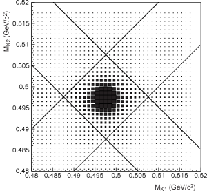
Figure 1: Reconstructed masses of the two $K^{0}_{S}$ candidates in data. The labels $K1$ and $K2$ are randomly assigned in each event. The diamond region near the center indicates the signal region.

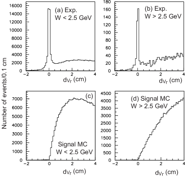
Figure 2: Distribution of $d_{Vr}$ (the signed distance between the two vertices in the $r\varphi$ plane) for the data (a,b) and MC (c,d) samples in two $W$ regions.

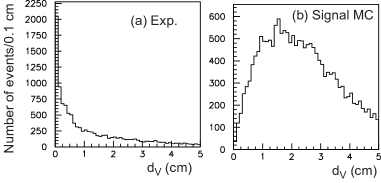
Figure 3: Distribution of $d_{V}$ (the distance of the two vertices in the three-dimensional space) for the data (a) and MC (b) samples.

Finally, the $p_{t}$ balance of the $K^{0}_{S}$ pair in the $e^{+}e^{-}$ c.m. frame is required to satisfy $|\sum\mbox{{\boldmath$p$}}_{t}^{*}|<0.1~{}{\rm GeV}/c$.

We select candidates in the region $1.05~{}{\rm GeV}\leq W\leq 4.10~{}{\rm GeV}$ and $|\cos\theta^{*}|<0.8$. The $W$ distribution of the selected $K^{0}_{S}K^{0}_{S}$ candidate events is shown in Fig. 4.

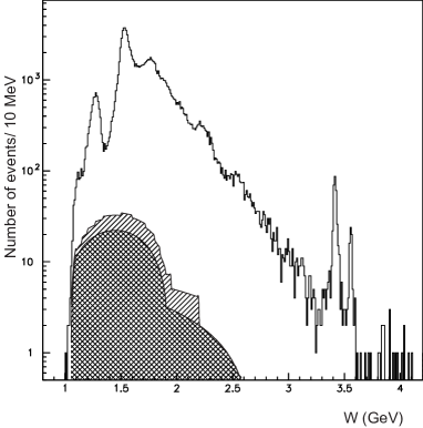
Figure 4: Distribution of $W$ for candidate events (solid histogram), as well as for the estimated non-exclusive background ($K^{0}_{S}K^{0}_{S}X$, cross hatched) and non-$K^{0}_{S}K^{0}_{S}$ four-pion background (hatched, modeled as a multi-step function). The requirement $|\cos\theta^{*}|<0.8$ is applied.

III Background subtraction

We first consider non-exclusive background of the type $K^{0}_{S}K^{0}_{S}X$, where $X$ is one or more particles. Then we discuss four-track events: $\pi^{+}\pi^{-}\pi^{+}\pi^{-}$ and $K^{0}_{S}K^{\pm}\pi^{\mp}$.

III.1 Non-exclusive background

The contamination by the non-exclusive background process, $K^{0}_{S}K^{0}_{S}X$, is estimated by fitting the $p_{t}$-balance ($|\sum\mbox{{\boldmath$p$}}_{t}^{*}|$) distribution with a function in which both the signal and background are considered in the region below 0.18 GeV/$c$. The region above 0.18 GeV/$c$ is not used in this estimate because the $p_{t}$-balance requirement effectively suppresses events in this region. We approximate the signal distribution with a function that is determined empirically from a signal MC study:

$$f_{s}(x)=\frac{Ax}{x^{\alpha}+Bx+C}\;,$$ (3)

where $x\equiv|\sum\mbox{{\boldmath$p$}}_{t}^{*}|$, $\alpha=1.56$ is determined from signal MC, and the parameters $A$, $B$ and $C$ are floated in the fits in each bin of $W$ and $|\cos\theta^{*}|$.

The background distribution is approximated with first- and second-order polynomials connected smoothly at $x=0.05$ GeV/$c$:

$$f_{b}(x) = ax\ \ \ \ \hskip 39.83385pt(x<0.05~{}{\rm GeV}/c)$$ (4)

$$= bx^{2}+cx+d\ \ \ (x\geq 0.05~{}{\rm GeV}/c).$$ (5)

We verify this approximation in our analyses of the $\pi^{0}\pi^{0}$ and $\eta\pi^{0}$ two-photon production where we observed a large amount of non-exclusive background of the same type pi0pi0 ; pi0pi02 ; etapi0 . The fit is performed for data in two-dimensional ($W$, $|\cos\theta^{*}|$) bins of width $\Delta W=0.1~{}$GeV (0.2 GeV) for $W$ below (above) 2.0 GeV and $\Delta|\cos\theta^{*}|=0.2$.

The results of several such fits are shown for the $0.2<|\cos\theta^{*}|<0.4$ region in Fig. 5. The background component is small in the signal region where the data are well described by our parameterization.

To extract the signal yields from data, we subtract the background contributions from our fits. The ($W$, $|\cos\theta^{*}|$) dependence of the background is approximated with a continuous function that is quadratic in most of the $W$ range (connected to linear in a subset of this range) and linear in $|\cos\theta^{*}|$. The background yields in each $W$ region, integrated over the angular bins, are shown in Fig. 4.

We estimate the systematic uncertainty associated with this background and its subtraction as half of the subtracted component. We add another 2% error in quadrature to account for the uncertainty in the background $p_{t}$ fit procedure.

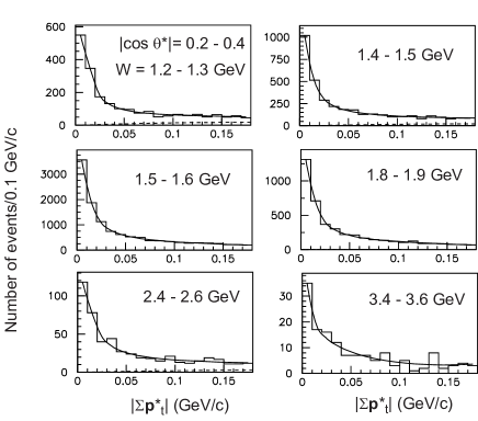
Figure 5: The $|\sum\mbox{{\boldmath$p$}}_{t}^{*}|$ distributions for several regions of $W$ in data for the angular region $0.2<|\cos\theta^{*}|<0.4$. The solid (dashed) curve shows the total (background) contribution obtained from the fit.

III.2 Non-$K^{0}_{S}K^{0}_{S}$ background – four-pion process

Background from the four-pion process is estimated using the summed yield in the $\langle M_{K}\rangle$ sideband regions, 0.4826–0.4876 GeV/$c^{2}$ and 0.5076–0.5126 GeV/$c^{2}$; the sum of the widths is the same as that for the signal region (0.4926–0.5026 GeV/$c^{2}$). We show $\langle M_{K}\rangle$ distributions for data in some $W$ regions in Fig. 6. The background contribution is appreciable in the region $W<2.2$ GeV only; as this background is always less than 1% for $W>2.2$ GeV, we incorporate the uncertainty in our estimate of this contribution in the systematic error but perform no subtraction in this $W$ region.

We obtain the $W$ distribution of the $\langle M_{K}\rangle$-sideband yields for the four separate $|\cos\theta^{*}|$ bins with a bin width of 0.2. To subtract the four-pion background, we approximate the ($W$, $|\cos\theta^{*}|$) dependence of the background with a multi-step function for $W$ (as shown in Fig. 4) and a linear function for $|\cos\theta^{*}|$.

If there were an overlap in the two kinds of backgrounds, i.e., if non-exclusive four-pion events ($\pi^{+}\pi^{-}\pi^{+}\pi^{-}X$) were to mimic the $K^{0}_{S}K^{0}_{S}X$ background, these contributions would be doubly counted and over-subtracted. We find no significantly large non-$K^{0}_{S}K^{0}_{S}(X)$ contribution in the $\langle M_{K}\rangle$ distribution for the $p_{t}$-unbalanced events with $0.1~{}{\rm GeV}/c<|\sum\mbox{{\boldmath$p$}}^{*}_{t}|<0.2~{}{\rm GeV}/c$, and therefore estimate the systematic uncertainty associated with the background subtraction as a half of the subtracted component. The possible effect of the overlap is included in this systematic uncertainty.

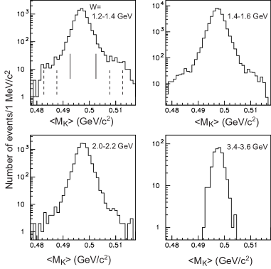
Figure 6: $\langle M_{K}\rangle$ data distributions for four $W$ regions. The vertical solid lines and the pairs of dashed vertical lines indicate the signal region and two sideband regions used for background subtraction, respectively.

III.3 Non-$K^{0}_{S}K^{0}_{S}$ background – $K^{0}_{S}K\pi$ process

The $K^{0}_{S}K^{\mp}\pi^{\pm}$ two-photon production, which has a cross section about ten times larger than that of the signal, would contaminate the signal sample if the charged kaon were misidentified as a pion.

According to our MC-based studies, the probability that a generated $K^{0}_{S}K\pi$ event is selected as a $K^{0}_{S}K^{0}_{S}$ signal candidate is smaller than $\sim 10^{-4}$ for $W>2.0$ GeV. This probability is so small because of the requirement on the decay vertex distances $r_{V1}$ and $r_{V2}$ imposed to reject this background.

We use two data-based methods to estimate the remaining $K^{0}_{S}K\pi$ background: from a study of the $r_{V}$ distributions near the IP and using our previous measurement of the $K^{0}_{S}K\pi$ production process nkzwc .

In the first method, we investigate the $r_{V}$ distribution after identifying one $K^{0}_{S}$ with a large $r_{Vj}$, $r_{Vj}>1$ cm on the opposite side. An excess of events near $r_{V}=0$ cm is observed in data for $W<2.0$ GeV/$c$. This is due to the $K^{0}_{S}K\pi$ background process, constituting between 0.1% and 4% of the sample at larger $r_{V}$. This component is observed primarily in the $W$ region below 1.5 GeV. The concentration of the background in the $W$ region may be partially due to four-pion final processes, where one pion track is misreconstructed, resulting in a fake reconstructed vertex. Since we do not separate the four-pion and $K^{0}_{S}K^{\mp}\pi^{\pm}$ backgrounds clearly in the low-$W$ region, we subtract this background assuming the contribution to be $2\%\pm 2\%$ of the signal in the $W$ region below 1.5 GeV. For $W>1.5~{}{\rm GeV}$, the excess in the $r_{V}$ distribution is small; this is supported by a study using the measurement of $K^{0}_{S}K\pi$ production.

In the second method, the observed yield from the process $\gamma\gamma\to K^{0}_{S}K\pi$ is an order of magnitude larger than that of the signal process for $W>2.5$ GeV nkzwc , but this background is suppressed by a factor of $\sim 1000$ in the data sample after our selection criteria are applied. Thus, it contributes less than 1% to the signal sample. We take this possible contamination into account as a systematic uncertainty of 1% for $W>1.5$ GeV.

IV Efficiency and efficiency corrections

In this section, we describe efficiency estimates including the factors from the L4 filter, triggers and $K^{0}_{S}K^{0}_{S}$ reconstruction. Then we discuss corrections for beam energy dependence.

IV.1 The L4 efficiency

Some loss of efficiency is introduced by the L4 software filter that is designed to suppress beam-gas and beam-wall events. Figure 7 shows the dependence of the L4 efficiency on $W$ for signal MC events that pass the trigger and all the selection criteria for an assumed isotropic angular dependence. The efficiency is significantly reduced for $W<1.1$ GeV and is stable, in the range between 80% and 94%, for $W>1.1$ GeV. For very low $W$, the inefficiency is dominated by the low reconstruction efficiency for tracks with small $p_{t}$; for high $W$, it is explained by tracks with large $dr$.

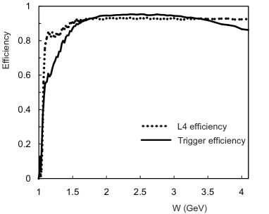
Figure 7: $W$ dependence of the L4 efficiency (dotted line) and trigger efficiency (solid line) estimated using the signal MC, where $K^{0}_{S}K^{0}_{S}$ were generated isotropically in the $\gamma\gamma$ c.m. frame at each $W$ point for the $W$ region 1.05 – 4.0 GeV. The L4 efficiency (trigger efficiency) is defined for the sample that passes through the trigger (L4) and all the selection criteria.

IV.2 Trigger efficiency

IV.2.1 Tuning of the simulator for trigger B

We tune the energy threshold for the ECL trigger (LowE), whose nominal value is 0.5 GeV, by comparing the efficiency curves of trigger B between the data and MC events in the four-pion process. With this tuning study in the trigger simulator (TSIM), the optimal value is determined to be 0.52 GeV.

In addition, we find a disagreement of about 20% between data and MC for the energy deposition in the ECL by a low-energy pion. As it is impractical to make dedicated changes in the trigger or detector simulation to describe the detector response to low-energy charged pions for this analysis, we have effectively shifted the LowE threshold by +110 MeV (to 0.63 GeV) to compensate for the pion-energy deposition mismatch.

This shift could affect the efficiency of the selection criterion based on $E_{\rm ECL}$. We study this possible effect and conclude that it is small, because of the loose criterion on $E_{\rm ECL}$. As our studies indicate that we could underestimate the efficiency by $\sim 1$% because of the ECL energy shift, we correct its value by this amount and assign 1% to the systematic uncertainty of this selection in the entire kinematic region.

IV.2.2 Estimation of the trigger efficiency

Using TSIM, we estimate the trigger efficiency for the combination of triggers A, B and C. Its validation using data is non-trivial, because we do not have mutually exclusive triggers to precisely measure the trigger efficiency from the data alone. We find that the contribution of trigger C to the combined efficiency is very small (0.3% – 2.0%, depending on $W$ and $|\cos\theta^{*}|$), so its contribution to the systematic error is negligible. To estimate the systematic uncertainty of the combined trigger efficiency, we study “trigger-A efficiency” $N({\rm A\cap B})/N({\rm B})$ and “trigger-B efficiency” $N({\rm A\cap B})/N({\rm A})$, where $N({\rm A\cap B})$ is the number of events recorded with both triggers, while $N({\rm B})$ ($N({\rm A})$) is that recorded with trigger B (A). These values represent the true trigger-A and -B efficiencies if triggers A and B are uncorrelated. Even though it is impossible to estimate the trigger correlation from data, it is useful to compare data and MC. We show the trigger-A and -B efficiencies in Fig. 8(a-d) for data and MC. In Fig. 8(e,f), the ratio $N({\rm B})/N({\rm A})$ is shown for data and MC. The figures are shown separately for the two angular regions, $|\cos\theta^{*}|=$ 0.0 – 0.4 and 0.4 – 0.8.

The difference in the angular distribution between the MC and data could cause an apparent deviation of the trigger efficiencies and their ratios in the comparison: in MC, we implement a flat distribution while, in data, steep changes of the distribution are seen for the small angles (typically, in $0.5<|\cos\theta^{*}|<0.8$) in some energy regions. To reduce this artifact in the plot for the region $0.4<|\cos\theta^{*}|<0.8$ (Fig. 8(b,d,f)), we subdivide the region into two bins with the same width, 0.2, and take an average for the two bins, for the trigger-A and -B efficiencies and the ratio. The trigger efficiencies estimated by the data and the MC simulation agree within 0.05 except for a low-statistics region. The assumption of flat angular distributions in MC introduces no bias in the efficiency calculation for cross section derivation because the efficiency is estimated on a bin-by-bin basis with a further narrow bin width, 0.05, in $|\cos\theta^{*}|$, whose resolution is much finer than the bin width, as described in Sec. IV.5.

In Fig. 7, we show the TSIM trigger efficiency as a function of $W$ for isotropically simulated MC events that satisfy the L4 and all other selection criteria in our analysis. The trigger efficiency rises steeply from 3% near $W=1.05$ GeV to 90% near $W=1.6$ GeV.

The systematic uncertainty of the trigger efficiency is estimated using the differences in the trigger-A and -B efficiencies and ratios between data and MC, taking into account the correlation between the triggers A and B as estimated from MC. It is evaluated to be 5%–7%, with a weak $W$ dependence.

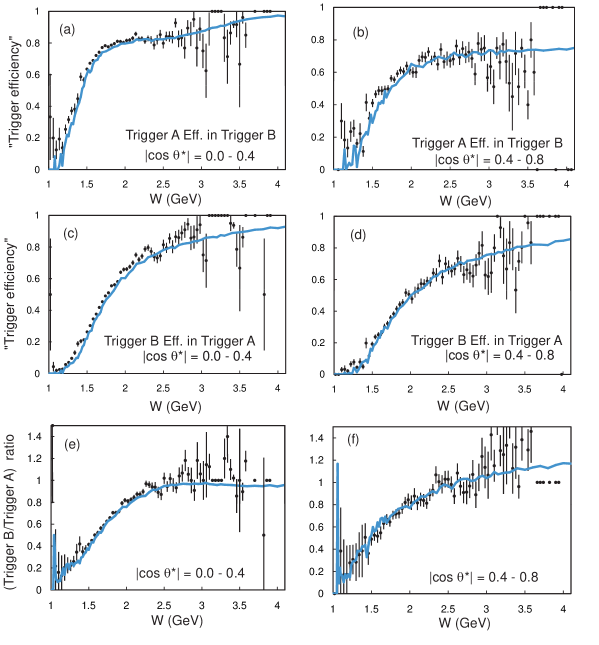
Figure 8: (a,b) The trigger-A efficiency and (c,d) the trigger-B efficiency (as defined in the text); (e,f) the ratio of the number of selected events from the two trigger samples, A and B. Data (dots with error bars) and signal MC (curves) samples are subdivided into the two $|\cos\theta^{*}|$ angular bins as labeled on the plots.

IV.2.3 Validation of the trigger efficiency

We compare our data with the results from the L3 experiment for the cross section of the $\gamma\gamma\to 4\pi$ process l34pi , where the $\pi^{+}\pi^{-}\pi^{+}\pi^{-}$ final-state includes $\rho^{0}\rho^{0}$ production but not $K^{0}_{S}K^{0}_{S}$ production. Ideally we would prefer to compare our results directly with $K^{0}_{S}K^{0}_{S}$ data obtained in previous experiments; however, no such high-statistics data are available. Figure 9 shows a comparison between Belle and L3 for the cross section of the four-pion process (excluding $K^{0}_{S}K^{0}_{S}$) at seven $W$ points (the $W$ bin widths being different between Belle and L3). The Belle selection for the four-pion process has a $p_{t}$ balance cut at 50 MeV/$c$ and non-exclusive backgrounds are subtracted using the $p_{t}$ distribution.

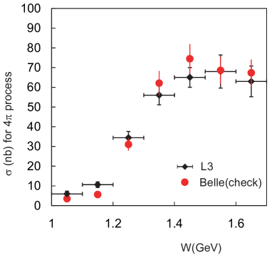
Figure 9: The measured cross section for the $\gamma\gamma\to\pi^{+}\pi^{-}\pi^{+}\pi^{-}$ process including $\rho^{0}\rho^{0}$ from Belle (closed circles) and L3 (diamonds) l34pi . The error bars include both statistical and systematic uncertainties, with a uniform 10% estimate used for Belle. These distributions are used solely for trigger-efficiency validation.

The relative systematic error of the Belle result is estimated to be 10%, while the statistical error is much smaller than that of L3. The Belle result is consistent with the L3 results, but no accurate comparison at a level better than 10% is possible. We assume the L3-determined fractions of the $\rho^{0}\rho^{0}$ components with spin 0 and 2. Note that the efficiency of the four-pion final state depends on this assumption.

IV.3 Reconstruction efficiency for the $K^{0}_{S}$ pair

The systematic error associated with the selection efficiency of the $K^{0}_{S}$ pairs is estimated by varying the selection criteria in the signal MC. When we do not find two $K^{0}_{S}$ candidates with our nominal criteria, we loosen the |$\Delta z$| criterion to $|\Delta z|<10$ cm, remove the requirements on $K^{0}_{S}$ vertices and loosen the requirement on $\langle M_{K}\rangle$ to $|\langle M_{K}\rangle-m_{K}|<10$  MeV/$c^{2}$, keeping all other criteria at their nominal values. These changes increase both signal efficiency and backgrounds, and we evaluate them with the same methods. The increase of the efficiency is 3%–10% (10%–20%) for $W>1.15$ GeV ($W<1.15$ GeV).

After the background subtraction, we use the differences in the fractional increase of the efficiency between the original and the loose cuts as its systematic uncertainty. It is difficult to evaluate backgrounds below $W<1.3$ GeV because the contamination is larger than the efficiency change and the two different types of non-$K^{0}_{S}K^{0}_{S}$ backgrounds are not well separated. As the systematic uncertainty is not expected to strongly depend on $W$, we assign 3% for $W<2.6$ GeV and 5% for $W>2.6$ GeV as the uncertainty in the efficiency reconstruction for the $K^{0}_{S}$ pairs.

Figure 10 shows the distribution of $\cos\theta$ (cosine of the laboratory angle) of $K^{0}_{S}$ for the signal candidates at $W=$1.7 – 1.9 GeV for the data and MC. Good agreement between the data and MC is obtained except for the forward-most bin ($\cos\theta>0.9$). The discrepancy there is due to the inadequate efficiency estimation, but its effect (about 3%) is within the systematic uncertainty from tracking, $K^{0}_{S}$ reconstruction and trigger efficiencies (see Sec. V).

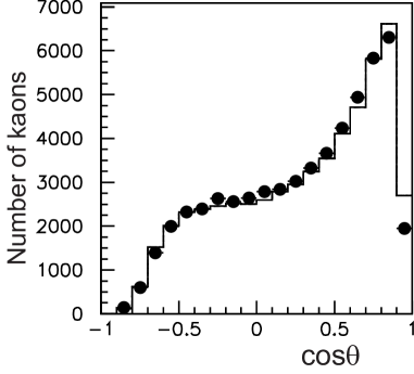
Figure 10: Distribution of $\cos\theta$ of $K^{0}_{S}$ in the $K^{0}_{S}K^{0}_{S}$ candidate events at $W=$ 1.7 – 1.9 GeV and $|\cos\theta^{*}|<0.8$ (two entries per event) for the data (dots) and MC (histogram). MC distribution is normalized to have the same number of kaons as observed in data.

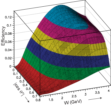
Figure 11: The overall efficiency vs. $W$ and $|\cos\theta^{*}|$.

IV.4 Beam energy dependence

The beam-energy dependence of the luminosity function and the efficiency is studied at the three energy points: $\Upsilon(4S)$ (10.58 GeV), $\Upsilon(5S)$ (10.88 GeV) and $\Upsilon(2S)$ (10.02 GeV), with the signal MC samples generated at each energy. We compare the luminosity function and efficiency at several $W$ points among the three beam energies. We use 10.58 GeV as the reference energy point and apply a correction proportional to the integrated luminosity to each sample at the other energies.

The luminosity function has a beam-energy dependence with a factor depending on $W$; for $W$ in (1.1 GeV, 2.0 GeV, 4.0 GeV), the factor is ($-5\%$, $-6\%$, $-10\%$) for 10.02 GeV and ($+2\%$, $+3\%$, $+5\%$) for 10.88 GeV. Meanwhile, the efficiency depends on the beam energy: $+3\%$ at 10.02 GeV and $-1\%$ at 10.88 GeV, which is opposite to the trend in the luminosity function. It is also weakly dependent on $W$.

The overall effect of the beam-energy differences is negligible when we apply the values of the efficiency and luminosity function for 10.58 GeV to all the data, and it is estimated to be at most 0.4% at any $W$. We do not correct for this effect and do not assign any systematic error.

IV.5 Invariant-mass and angular resolution

We estimate a $K^{0}_{S}K^{0}_{S}$ mass resolution (i.e., a $W$ resolution) of $\sigma_{W}/W=0.2\%$ for the entire $W$ region, with a small $W$ dependence, according to a signal MC study. As this is much smaller than the bin width (at worst, $\sigma_{M}<4$ MeV near $W=1.9$ GeV, where the bin width is 10 MeV), we do not apply unfolding. The estimated systematic shift due to bin migrations associated with resolution is less than 1% and is absorbed in the systematics.

The resolution for the c.m. angle measurement in each event is typically $\sigma_{|\cos\theta^{*}|}=0.0025$, which is much smaller than the bin width of 0.1.

V Differential cross section

The differential cross section $d\sigma/d|\cos\theta^{*}|$ is derived after the subtraction of the backgrounds and the application of the corrections to the yields and efficiencies:

$$\frac{d\sigma}{d|\cos\theta^{*}|} = \frac{1}{\int{\cal L}dt\ L_{\gamma\gamma}\ \Delta W\ \Delta|\cos\theta^{*}|}\times$$ (6)

$$\frac{N-N_{\rm bkg}}{\epsilon\ {\cal B}(K^{0}_{S}\to\pi^{+}\pi^{-})^{2}}\;,$$

where $N$ ($N_{\rm bkg}$) is the number of candidate (background) events, $\int{\cal L}dt$ is the total integrated luminosity and $L_{\gamma\gamma}$ is the two-photon luminosity function, calculated as a function of $W$. $\Delta W$ and $\Delta|\cos\theta^{*}|$ are the bin widths, and $\epsilon$ is the efficiency that includes all trigger/selection effects. The $W$ and $|\cos\theta^{*}|$ dependence of the overall efficiency is shown in Fig. 11. The efficiency is smaller than 0.14 everywhere in the measurement range. A major cause of the overall efficiency loss is associated with a Lorentz boost of the two-photon system which results in at least one $K^{0}_{S}$ falling outside of the detector’s acceptance typically more than half of the time. Note that this efficiency loss strongly depends on $W$ and $|\cos\theta^{*}|$.

We extract the differential cross section in the range $|\cos\theta^{*}|<0.8$ and 1.1 GeV$<W<3.3$ GeV, with a $W$ bin width of 10 MeV for $W=1.1-1.9$ GeV, 20 MeV for 1.9 – 2.4 GeV, 40 MeV for 2.4 – 2.6 GeV, and 100 MeV for 2.6 – 3.3 GeV. In this extraction, we first evaluate the differential cross section for finer bin widths, $\Delta W=10$ MeV and $\Delta|\cos\theta^{*}|=0.05$ over the entire region, using the efficiency for the central point of each bin. The values for these fine bins are then combined via a weighted average into the coarser bins, with a weight calculated from the statistical errors.

In the range $W=1.05-1.10$ GeV, we extract only the cross section integrated over $|\cos\theta^{*}|<0.6$, assuming a flat angular dependence of the differential cross section because of limited statistics and the limited coverage in the forward angles in the vicinity of $|\cos\theta^{*}|\sim 0.6$.

In the range $W=3.3-3.6$ GeV, we do not extract the $\gamma\gamma\to K^{0}_{S}K^{0}_{S}$ cross section where the contributions from the $\chi_{c0}$ and $\chi_{c2}$ resonances dominate the yield; we cannot subtract leakages from these narrow states reliably over the entire region.

In the range $W=3.6-4.0$ GeV, we find some contribution from the signal process. It is possible to extract the integrated cross section for $|\cos\theta^{*}|<0.8$ in this $W$ region; however, we do not present differential cross section due to small statistics. There could be a contribution from high-mass charmonium resonance(s) ($\chi_{cJ}(2P)$ for example) at $W=3.80-3.95$ GeV, as we find some events at large angles in this $W$ range; these events are included in the total cross section (see Fig. 28).

At $W=4.0-4.1$ GeV, we find only a small number of signal events that give a peak near $|\sum\mbox{{\boldmath$p$}}^{*}_{t}|=0$, consistent with a large background contamination. No cross section measurement is therefore performed in the $W$ region above 4.0 GeV.

Figure 12 shows the cross section integrated over $|\cos\theta^{*}|$. The integration is performed by summing the differential cross section for $|\cos\theta^{*}|<0.8$ or $|\cos\theta^{*}|<0.6$. The error bars are statistical only. The curves in the figure show the total systematic errors.

Figure 12: The $W$ dependence of the $\gamma\gamma\to K^{0}_{S}K^{0}_{S}$ cross section after integrating over the angle up to (a,b) $|\cos\theta^{*}|<0.8$ (black points) and (c,d) $|\cos\theta^{*}|<0.6$ (blue points). The orange square markers in (d) are from our previous publication chen for $|\cos\theta^{*}|<0.6$. The solid curves are the systematic uncertainties.

The systematic error includes contributions from the uncertainties in tracking efficiency (2% for 4 tracks), beam-background effects (1%) estimated from the stability of yield ratios between the data and MC across all run periods, pion identification (2% for four pions), non-exclusive and four-pion backgrounds (described in Sec. III.1 and B), geometrical coverage and fit uncertainty (4% in total), $K^{0}_{S}K\pi$ background subtraction (Sec. III.3), $K^{0}_{S}$-pair reconstruction (Sec. IV.3), trigger efficiency (Sec. IV.2), and the $E_{\rm ECL}$ cut (Sec. IV.2). We assign the uncertainty for the L4 efficiency to be about 10% of the inefficiency in different $W$ regions. The systematic error associated with the uncertainty in the integrated luminosity and luminosity function includes the form-factor effect of space-like photons. Summing in quadrature, the total systematic uncertainty evaluated is typically 10%. The systematic uncertainties are summarized in Table 1.

Table 1: Summary of systematic uncertainties (%) in the cross section integrated over the angle in a single $W$ bin. When a range is shown, the uncertainty varies between the values with decreasing $W$.

Source	Uncertainty (%)
Tracking efficiency (for 4 tracks)	2
Beam background effect	1
Pion identification (for 4 tracks)	2
Non-exclusive and four-pion backgrounds	2 – 19
Geometrical coverage and fit uncertainty	4
$K^{0}_{S}K\pi$ background subtraction	1 – 2
$K^{0}_{S}$-pair reconstruction	5 – 3
Trigger efficiency	5 – 7
$E_{\rm ECL}$ cut	1
Integrated luminosity and luminosity function	5 – 4
L4 efficiency	1 – 10
Total	9 – 25, typically 10

VI Study of resonances

Figure 12(a) shows the measured integrated cross section ($|\cos\theta^{*}|\leq 0.8$), where prominent peaks are observed near 1.3, 1.5 and 1.8 GeV. Enhancements are also observed around 2.3 and 2.6 GeV. A close-up view of the integrated cross section ($|\cos\theta^{*}|\leq 0.6$) near the threshold is shown in Fig. 13, where the cross section is small ($<1$ nb), in agreement with theoretical predictions achasov ; achasov2 .

In this section we describe the extraction of partial wave information from our data by fitting the differential cross section using suitable parameterizations to estimate the mass, total width and $\Gamma_{\gamma\gamma}{\cal B}(K\bar{K})$ of the $f_{2}^{\prime}(1525)$, to derive the phase difference between the $f_{2}(1270)$ and $a_{2}(1320)$ and to identify the nature and obtain the parameters of the resonances near 1.8, 2.3 and 2.6 GeV.

Figure 13: A close-up view of the measured integrated cross section ($|\cos\theta^{*}|\leq 0.6$) near the threshold for the process $\gamma\gamma\to K^{0}_{S}K^{0}_{S}$. The solid curve is the systematic uncertainty.

VI.1 Partial wave amplitudes

In the $\gamma\gamma\to K^{0}_{S}K^{0}_{S}$ channel, only the partial waves of even angular momenta contribute. Furthermore, in the energy region $W\stackrel{{\scriptstyle<}}{{\sim}}3~{}{\rm GeV}$, the $J>4$ partial waves may be ignored, so only S, D and G waves are considered in the fit. The differential cross section can then be expressed as

$$\frac{d\sigma(\gamma\gamma\to K^{0}_{S}K^{0}_{S})}{d\Omega} = \left|S\>Y^{0}_{0}+D_{0}\>Y^{0}_{2}+G_{0}\>Y^{0}_{4}\right|^{2}$$ (7)

$$+\left|D_{2}\>Y^{2}_{2}+G_{2}\>Y^{2}_{4}\right|^{2}\;,$$

where $S$ is the S-wave amplitude, $D_{0}$ and $G_{0}$ ($D_{2}$ and $G_{2}$) denote the helicity-0 (2) components of the D and G wave pw , respectively, and $Y^{m}_{J}$ are the spherical harmonics. The angular dependence of the cross section is governed by the spherical harmonics while the energy dependence is determined by the partial waves.

Since the spherical harmonics are not independent of each other, a unique decomposition of partial waves cannot be determined using the measured differential cross section. To overcome this problem, we rewrite Eq. (7) as

$$\frac{d\sigma(\gamma\gamma\to K^{0}_{S}K^{0}_{S})}{4\pi d|\cos\theta^{*}|} = \hat{S}^{2}\>|Y^{0}_{0}|^{2}+\hat{D}_{0}^{2}\>|Y^{0}_{2}|^{2}+\hat{D}_{2}^{2}\>|Y^{2}_{2}|^{2}\,$$ (8)

$$+\hat{G}_{0}^{2}\>|Y^{0}_{4}|^{2}\,+\hat{G}_{2}^{2}\>|Y^{2}_{4}|^{2}\,.$$

The “hat-amplitudes” $\hat{S}^{2}$, $\hat{D}_{0}^{2}$, $\hat{D}_{2}^{2}$, $\hat{G}_{0}^{2}$ and $\hat{G}_{2}^{2}$ can be negative because of interference terms, and correspond to $|S|^{2},\;|D_{0}|^{2},\;|D_{2}|^{2},\;|G_{0}|^{2}$ and $|G_{2}|^{2}$, respectively, when interference terms are ignored pi0pi0 .

As the absolute squares of the spherical harmonics are independent of each other, we can fit the differential cross section in each $W$ bin to obtain $\hat{S}^{2}$, $\hat{D}_{0}^{2}$, $\hat{D}_{2}^{2}$, $\hat{G}_{0}^{2}$ and $\hat{G}_{2}^{2}$. The fit with the value of $J\leq 4$ is named the “$SDG$ fit.” At low energy, we expect that the contribution from $J=4$ is negligible, so we also perform a separate fit by setting $\hat{G}_{0}^{2}=\hat{G}_{2}^{2}=0$, which is named the “$SD$ fit.”

The differential cross section is fitted according to Eq. (8), where statistical errors only are taken into account. The differential cross section for $|\cos\theta^{*}|\leq 0.8$ is extracted for $1.1~{}{\rm GeV}\leq W\leq 3.3~{}{\rm GeV}$. In the $SDG$ fit, two consecutive data points of $\Delta W=0.01$ GeV are merged, resulting in bins of width 0.02 GeV.

The obtained spectra of $\hat{S}^{2}$, $\hat{D}_{0}^{2}$ and $\hat{D}_{2}^{2}$ for the $SD$ fit are shown in Fig. 14. Figures 15 and 16 show the hat-amplitudes for the $SDG$ fit. $\hat{G}_{0}^{2}\pm\hat{G}_{2}^{2}$ are also plotted in Fig. 16, since the angular dependences of $|Y^{0}_{4}|^{2}$ and $|Y^{2}_{4}|^{2}$ are similar for $|\cos\theta^{*}|\stackrel{{\scriptstyle<}}{{\sim}}0.6$. In the $SDG$ fit, the structures in $\hat{D}_{2}^{2}$ are less visible and the G waves appear to be small for $W\leq 3.3$ GeV. Figure 17 shows the differential cross section for selected $W$ bins with the fitted $\hat{S}$, $\hat{D}_{0}$ and $\hat{D}_{2}$ waves.

Figure 14: Amplitudes $\hat{S}^{2}$ (left top), $\hat{D}_{0}^{2}$ (left bottom) and $\hat{D}_{2}^{2}$ (right) obtained from the $SD$ fit. The error bars represent the statistical uncertainties when no correlations among the fit parameters are included.

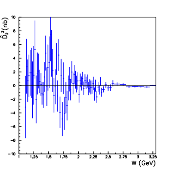
Figure 15: Amplitudes $\hat{S}^{2}$ (left top), $\hat{D}_{0}^{2}$ (left bottom) and $\hat{D}_{2}^{2}$ (right) obtained from the $SDG$ fit. The error bars represent the statistical uncertainties when no correlations among the fit parameters are included.

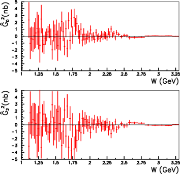
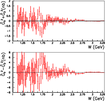
Figure 16: Amplitudes $\hat{G}_{0}^{2}$ (left top), $\hat{G}_{2}^{2}$ (left bottom) and $\hat{G}_{0}^{2}\pm\hat{G}_{2}^{2}$ (right) obtained from the $SDG$ fit. The error bars represent the statistical uncertainties when no correlations among the fit parameters are included.

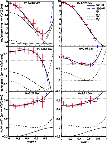
Figure 17: Results of the $SD$- (solid line) and $SDG$- (long-dashed line) fits of the differential cross section in selected $W$ bins. The number in each panel denotes the $W$ bin. Also shown are $\hat{S}^{2}$ (dotted line), $\hat{D}_{0}^{2}$ (dashed line) and $\hat{D}_{2}^{2}$ (dot-dashed line) obtained from the $SD$ fit.

Although the derived hat-amplitudes $\hat{S}^{2}$, $\hat{D}_{0}^{2}$, $\hat{D}_{2}^{2}$, $\hat{G}_{0}^{2}$ and $\hat{G}_{2}^{2}$ in fact contain interference terms such as $\Re(S^{*}D_{0})$, they do provide useful information about partial wave amplitudes. Two prominent peaks are observed in the $\hat{D}_{2}^{2}$ spectrum: the peak near 1.3 GeV is due to the interference between the $f_{2}(1270)$ and $a_{2}(1320)$ and the second peak is due to the $f_{2}^{\prime}(1525)$. No other notable structures are observed in Fig. 14 (right). In the $\hat{S}^{2}$ spectrum shown in Fig. 14 (left top), three peaks around 1.8, 2.3 and 2.6 GeV are observed. The lowest may be due to the $f_{0}(1710)$ (not a tensor meson, as discussed in past experiments tasso1 ; L3 ; kabe ). This might be an $a_{0}$ meson, though no such mesons have been observed previously in this mass region pdg2012 . $\hat{D}_{0}^{2}$ is rather small and featureless except around 2.1 and 2.6 GeV, and hence the D₀ wave may also be small but non-zero: there appears to be an interference term between S and D₀.

We use our assumptions for the partial wave amplitudes and fit the data to extract the parameters of the resonances. Note that we do not fit the obtained spectra of hat-amplitudes $\hat{S}^{2}$, $\hat{D}_{0}^{2}$ and $\hat{D}_{2}^{2}$, but rather fit the differential cross section directly using Eq. (7). In our analysis, we fit the energy region $W\leq 3.0~{}{\rm GeV}$, with separate fits for $W\leq 2$ GeV and $W>2$ GeV.

VI.2 Fitting the region $W\leq 2.0~{}{\rm GeV}$

In this section, we describe our fits in the $W\leq 2.0$ GeV region. Motivated by the spectra of $\hat{D}_{2}^{2}$ and $\hat{S}^{2}$, we include the $f_{2}(1270)$, $a_{2}(1320)$ and $f_{2}^{\prime}(1525)$ in the D₂ wave and test the hypothesis of a scalar meson (coined the $f_{0}(1710)$) in the S wave. In this analysis, we measure the relative phase probing the destructive interference between the $f_{2}(1270)$ and $a_{2}(1320)$ and determine relevant parameters of the $f_{2}^{\prime}(1525)$, in particular, $\Gamma_{\gamma\gamma}{\cal B}(K\bar{K})$.

VI.2.1 Parameterization of amplitudes

Based on the above observation, the amplitudes $S$, $D_{0}$ and $D_{2}$ are parameterized as follows:

$$S = A_{f_{0}(1710)}e^{i\phi_{f0}}+B_{S},$$

$$D_{0} = B_{D0}e^{i\phi_{D0}},$$

$$D_{2} = A_{f_{2}(1270)}+A_{a_{2}(1320)}e^{i\phi_{a2}}+A_{f_{2}^{\prime}(1525)}e^{i\phi_{f2p}}$$ (9)

$$+B_{D2}e^{i\phi_{D2}},$$

where $A_{f_{0}(1710)}$, $A_{f_{2}(1270)}$, $A_{a_{2}(1320)}$ and $A_{f_{2}^{\prime}(1525)}$ are the amplitudes describing the resonances; $B_{S}$, $B_{D0}$ and $B_{D2}$ are the non-resonant background amplitudes for the S, D₀ and D₂ waves; and $\phi_{f0}$, $\phi_{a2}$, $\phi_{f2p}$, $\phi_{D0}$ and $\phi_{D2}$ are the phases of the resonances and background amplitudes. The phases are defined relative to $B_{S}$ ($f_{2}(1270)$) for helicity-0 (2) amplitudes. Using this convention, the relative phase between the $f_{2}(1270)$ and $a_{2}(1320)$ is given by $\phi_{a2}$. We also study the case in which the $f_{0}(1710)$ is replaced by a tensor meson (labeled the $f_{2}(1710)$ here, although the $f_{2}(1810)$ is listed in PDG pdg2012 ) in $D_{2}$. To investigate if our approximation could describe the data well without this resonant contribution, we also perform a fit assuming no resonance at 1.8 GeV.

We assume the background amplitudes to be quadratic in $W$ multiplied by the threshold factor $\beta^{2l+1}$ for all waves:

$$B_{S} = \beta(a_{S}W^{\prime 2}+b_{S}W^{\prime}+c_{S})\;,$$

$$B_{D0} = \beta^{5}(a_{D0}W^{\prime 2}+b_{D0}W^{\prime}+c_{D0})\;,$$

$$B_{D2} = \beta^{5}(a_{D2}W^{\prime 2}+b_{D2}W^{\prime}+c_{D2})\;,$$ (10)

where $W^{\prime}=W-2m_{K^{0}_{S}}$, $\beta=\sqrt{1-4m_{K^{0}_{S}}^{2}/W^{2}}$ is the velocity of the $K^{0}_{S}$ divided by the speed of light, $m_{K^{0}_{S}}$ is the mass of the $K^{0}_{S}$, and $l$ is 0 (2) for $S$ ($D_{0}$ and $D_{2}$).

We use the parameterization of the $f_{2}(1270)$ and $f_{2}^{\prime}(1525)$ given in Ref. pi0pi0 and that of the $a_{2}(1320)$ in Ref. etapi0 . We note that ${{\cal B}}(R\rightarrow K^{0}_{S}K^{0}_{S})/{{\cal B}}(R\rightarrow K\bar{K})=1/4$ for any $f_{J}$ or $a_{J}$ resonance $R$.

The amplitude $A_{R}(W)$ for each spin-$J$ resonance $R$ of mass $m_{R}$ is parameterized using the relativistic Breit-Wigner formula

$$A_{R}^{J}(W) = \sqrt{\frac{8\pi(2J+1)m_{R}}{W}}$$ (11)

$$\times\frac{\sqrt{\Gamma_{\rm tot}(W)\Gamma_{\gamma\gamma}(W){\cal B}(K\bar{K}})}{m_{R}^{2}-W^{2}-im_{R}\Gamma_{\rm tot}(W)}\;.$$

Hereinafter, we consider the case $J=2$. The energy-dependent total width $\Gamma_{\rm tot}(W)$ is given by

$$\Gamma_{\rm tot}(W)=\sum_{X_{1}X_{2}}\Gamma_{X_{1}X_{2}}(W)\;,$$ (12)

where $X_{1},\;X_{2}$ is $\pi$, $K$, $\eta$, $\gamma$, etc. For $J=2$, the partial width $\Gamma_{X_{1}X_{2}}(W)$ is parameterized as blat :

$$\Gamma_{X_{1}X_{2}}(W) = \Gamma_{R}{\cal B}(R\rightarrow X_{1}X_{2})\left(\frac{q_{X}(W^{2})}{q_{X}(m_{R}^{2})}\right)^{5}$$ (13)

$$\times\frac{D_{2}\left(q_{X}(W^{2})r_{R}\right)}{D_{2}\left(q_{X}(m_{R}^{2})r_{R}\right)}\;,$$

where $\Gamma_{R}$ is the total width at the resonance mass,

$$q_{X}(W^{2}) = \frac{1}{2W}\left[\left(W^{2}-(m_{X_{1}}+m_{X_{2}})^{2}\right)\right.$$

$$\times\left.\left(W^{2}-(m_{X_{1}}-m_{X_{2}})^{2}\right)\right]^{\frac{1}{2}},$$

$$D_{2}(x) = \frac{1}{9+3x^{2}+x^{4}}\;,$$ (14)

and $r_{R}$ is an effective interaction radius that varies from 1 $({\rm GeV}/c)^{-1}$ to 7 $({\rm GeV}/c)^{-1}$ in different hadronic reactions grayer ; grayer2 ; grayer3 . For the three-body and other decay modes,

$$\Gamma_{\rm other}(W)=\Gamma_{R}{\cal B}(R\rightarrow{\rm other})\frac{W^{2}}{m_{R}^{2}}$$ (15)

is used instead of Eq. (13). This formalism is used for the $f_{2}(1270)$, $a_{2}(1320)$ and $f_{2}^{\prime}(1525)$. All parameters of the $f_{2}(1270)$ and $a_{2}(1320)$ are fixed at the PDG values pdg2012 except for $r_{R}$, which is fixed at the value determined in Refs. mori1 ; mori2 , as summarized in Tables 2 and 3.

Table 2: A summary of the parameters assumed in our fits.

Parameter	$f_{2}\left(1270\right)$	$f_{2}^{\prime}\left(1525\right)$	Unit	Reference
Mass	$1275.1\pm 1.2$	$1525\pm 5$	${\rm MeV}/c^{2}$	pdg2012
$\Gamma_{\rm tot}$	$185.1^{+2.9}_{-2.4}$	$73^{+6}_{-5}$	MeV	pdg2012
${\cal B}(\pi\pi)$	$84.8^{+2.4}_{-1.2}$	$0.82\pm 0.15$	%	pdg2012
${\cal B}(K\bar{K})$	$4.6\pm 0.4$	$88.7\pm 2.2$	%	pdg2012
${\cal B}(\eta\eta)$	$0.40\pm 0.08$	$10.4\pm 2.2$	%	pdg2012
${\cal B}(\gamma\gamma)$	$16.4\pm 1.9$	$1.11\pm 0.14$	$10^{-6}$	pdg2012
$r_{R}$	$3.62\pm 0.03$	$3.62\pm 0.03$	$({\rm GeV}/c)^{-1}$	mori1 ; mori2

Table 3: Parameters of the $a_{2}(1320)$ pdg2012 .

Parameter	Value	Unit
Mass	$1318.3\pm 0.6$	${\rm MeV}/c^{2}$
$\Gamma_{\rm tot}$	$107\pm 5$	MeV
${\cal B}(\rho\pi)$	$70.1\pm 2.7$	%
${\cal B}(\eta\pi)$	$14.5\pm 1.2$	%
${\cal B}(\omega\pi\pi)$	$10.6\pm 3.2$	%
${\cal B}(K\bar{K})$	$4.9\pm 0.8$	%
${\cal B}(\gamma\gamma)$	$9.4\pm 0.7$	$10^{-6}$

Finally, the parameterization of the $f_{0}(M)$ meson for $M=1710~{}{\rm MeV}/c^{2}$ is taken to be:

$$f_{0}(M)=\sqrt{\frac{8\pi m_{f_{0}}}{W}}\frac{\sqrt{\Gamma_{f_{0}}\Gamma_{\gamma\gamma}{\cal B}(K\bar{K})_{f_{0}}}}{m^{2}_{f_{0}}-W^{2}-im_{f_{0}}\Gamma_{f_{0}}}\;,$$ (16)

where $\Gamma_{\gamma\gamma}{\cal B}(K\bar{K})_{f_{0}}$ is the product of the two-photon width and the branching fraction to $K\bar{K}$ for the $f_{0}(M)$ meson. Its PDG pdg2012 parameters are summarized in Table 4, together with the parameters (when known) of the $f_{2}(1810)$ and $a_{2}(1700)$.

Table 4: Parameters (when known) of the $f_{0}(1710)$, $a_{2}(1700)$ and $f_{2}(1810)$ pdg2012 .

Parameter	$f_{0}(1710)$	$a_{2}(1700)$	$f_{2}(1810)$
Mass (MeV/$c^{2}$ )	$1720\pm 6$	$1732\pm 16$	$1815\pm 12$
$\Gamma_{\rm tot}$ (MeV)	$135\pm 8$	$194\pm 40$	$197\pm 22$
$f_{J}/a_{J}\to K\bar{K}$	seen	seen	unknown
$f_{J}/a_{J}\to\gamma\gamma$	unknown	unknown	seen

VI.2.2 Fit in the region $1.2~{}{\rm GeV}\leq W\leq 2.0~{}{\rm GeV}$

We perform a fit for the region $1.2~{}{\rm GeV}\leq W\leq 2.0~{}{\rm GeV}$ by floating the mass, width, $\Gamma_{\gamma\gamma}{\cal B}(K\bar{K})$ and the relative phase of both the $f_{2}^{\prime}(1525)$ and $f_{J}(1710)$ ($J=0$ or $J=2$). Also floated are the relative phase of the $a_{2}(1320)$ and the parameters ($a,\;b$ and $c$ and the phases for $D_{0}$ and $D_{2}$) of the background amplitudes. To remove arbitrary sign uncertainties, the coefficients $c_{S}$, $c_{0}$ and $c_{2}$ are chosen to be positive.

Twenty parameters describing the assumed amplitudes are obtained by fitting the differential cross sections. To search for the global minimum goodness of fit $\chi^{2}_{\rm min}$ to identify possible multiple solutions, about 1000 sets of randomly generated initial parameters are employed for fits performed using MINUIT minuit . A fit is accepted as a satisfactory solution if its $\chi^{2}$-value is within $\chi^{2}_{\rm min}+10$ (corresponding to $3.2\sigma$).

If the $f_{0}(1710)$ hypothesis is assumed to explain the peak at $W\sim 1.8~{}{\rm GeV}$, four solutions are obtained with $\chi^{2}_{\rm min}/ndf=677.2/580$, where $ndf$ is the number of degrees of freedom. These solutions are distinguished by the $\Gamma_{\gamma\gamma}{\cal B}(K\bar{K})$ value, which ranges from 6.3 to 216 eV for the $f_{0}(1710)$, and from 83 to 104 eV for the $f_{2}^{\prime}(1525)$, as listed in Table 5.

When the $f_{2}(1710)$ hypothesis is used, the two obtained solutions have lower quality with $\chi^{2}_{\rm min}/ndf=755.6/580$. Their fitted values are also listed in Table 5. As the $f_{0}(1710)$ solutions have lower $\chi^{2}_{\rm min}/ndf$, they are favored over the $f_{2}(1710)$.

We conclude that the region $1.2~{}{\rm GeV}\leq W\leq 2.0~{}{\rm GeV}$ is too wide to fit in extracting the desired parameters at once. We therefore fit individual parameters one at a time, keeping in mind the limitations of this approach.

Table 5: Solutions of the $f_{J}(W\leq 2~{}{\rm GeV})$ fit.

Fit	$f_{0}(W\leq 2~{}{\rm GeV})$ fit				$f_{2}(W\leq 2~{}{\rm GeV})$ fit
Sol.	1	2	3	4	1	2
$\chi^{2}$ ($ndf=580$)	677.2	682.3	685.4	686.7	755.6	759.6
$\phi_{a2}$ (deg.)	178.3	184.7	183.8	178.7	183.2	180.3
Mass$(f_{2}^{\prime})$ (MeV$/c^{2}$)	1527.9	1527.2	1527.7	1526.1	1527.9	1527.5
$\Gamma_{\rm tot}(f_{2}^{\prime})$ (MeV)	85.5	86.3	85.8	81.5	85.5	83.5
$\Gamma_{\gamma\gamma}{\cal B}(K\bar{K})_{f_{2}^{\prime}}$ (eV)	82.8	103.8	85.8	90.0	89.0	127.1
$\phi_{f2p}$ (deg.)	277	250	242	211	251	288
Mass$(f_{0})$ (MeV$/c^{2}$)	1781	1780	1783	1761	1793	1782
$\Gamma_{\rm tot}(f_{0})$ (MeV)	99	110	96	119	93	104
$\Gamma_{\gamma\gamma}{\cal B}(K\bar{K})_{f_{0}}$ (eV)	216	6.3	189	10.3	89.0	127
$\phi_{f0}$ (deg.)	264	125	265	90	251	288

VI.2.3 The “$f_{2}^{\prime}(1525)$ fit”

Based on the above observation, we first obtain the $f_{2}^{\prime}(1525)$ parameters by fitting the c.m. energy range $1.15~{}{\rm GeV}\leq W\leq 1.65~{}{\rm GeV}$ and ignoring the contribution of the $f_{J}(1710)$. The differential cross section is fit with the parameterized amplitudes by floating the $f_{2}^{\prime}(1525)$ parameters as well as the relative phase between the $a_{2}(1320)$ and $f_{2}(1270)$. Hereinafter, this fit is referred to as the “$f_{2}^{\prime}(1525)$ fit.” The background amplitudes are approximated with linear functions because the fitting range is rather narrow. There are thirteen parameters to extract from this fit.

Two solutions are obtained, both with $\chi^{2}/ndf=0.97$. The main difference between the two solutions is the values of $\Gamma_{\gamma\gamma}{\cal B}(K\bar{K})$ for the $f_{2}^{\prime}(1525)$: 113 and 48 eV, with the two solutions referred to as H (high) and L (low), respectively. They correspond to destructive and constructive interference between the $f_{2}^{\prime}(1525)$ and non-resonant $D_{2}$ background. The fitted results are shown in Figs. 18 and 19 for the H and L solutions, respectively. The fitted values are listed and compared with those of PDG pdg2012 in Table 6. The quoted errors are MINOS statistical errors, determined by evaluating the parameter values that give $\chi^{2}_{\rm min}+1$ for each variable being studied. In the fit, all other parameters are floated. In both solutions, the interference between the $f_{2}(1270)$ and $a_{2}(1320)$ is indeed destructive as predicted lipkin , i.e., the measured $\phi_{a2}$ is close to $180^{\circ}$.

We stress that the previous measurements of $\Gamma_{\gamma\gamma}{\cal B}(K\bar{K})$ for the $f_{2}^{\prime}(1525)$ L3 assumed no interference. In order to check the consistency with past experiments, an incoherent fit is also performed, where we replace $|D_{2}Y_{2}^{2}|^{2}$ with $|(D_{2}-A_{f_{2}^{\prime}(1525)}e^{i\phi_{f2p}})Y_{2}^{2}|^{2}+|A_{f_{2}^{\prime}(1525)}Y_{2}^{2}|^{2}$ in Eq. (7). The obtained value of $\Gamma_{\gamma\gamma}{\cal B}(K\bar{K})$ is $79.1\pm 1.4$ eV, which is consistent with $76\pm 6\pm 11$ eV reported by L3 L3 , $110^{+30}_{-20}\pm 20$ eV by CELLO cello , $100^{+40+30}_{-30-20}$ eV by PLUTO pluto and $110\pm 20\pm 40$ eV by TASSO tasso1 . The results of our fits are also shown in Table 6.

Table 6: Parameters obtained from the $f_{2}^{\prime}(1525)$ fit and incoherent fit. For the H and L solutions, the first error is statistical and the second systematic (itemized in Table 7). The parameters where the H and L solutions are combined are also shown (explained in Sec. VI.2.5).

Parameter	Solution H	Solution L	H, L combined	Incoherent fit	PDG pdg2012
$\chi^{2}/ndf$	375.09/387	375.22/387	–	406.6/388	–
$\phi_{a_{2}(1320)}$ (deg.)	$178.1^{+1.7+6.7}_{-1.3-12.5}$	$172.6^{+1.3+6.7}_{-1.0-3.1}$	$172.6^{+6.0+12.2}_{-0.7-7.0}$	$173.6^{+1.3}_{-1.4}$	–
Mass$(f_{2}^{\prime}(1525))$ (MeV/$c^{2}$)	$1526.1^{+0.9+2.9}_{-1.0-2.8}$	$1524.3^{+1.0+1.6}_{-0.9-1.1}$	$1525.3^{+1.2+3.7}_{-1.4-2.1}$	$1530.7\pm 0.4$	$1525\pm 5$
$\Gamma_{\rm tot}(f_{2}^{\prime}(1525))$ (MeV)	$83.4^{+1.9+2.0}_{-1.7-3.4}$	$81.8^{+2.3+4.4}_{-2.0-0.9}$	$82.9^{+2.1+3.3}_{-2.2-2.0}$	$82.7\pm 1.4$	$73^{+6}_{-5}$
$\Gamma_{\gamma\gamma}{\cal B}(K\bar{K})(f_{2}^{\prime}(1525))$ (eV)	$113^{+25+43}_{-28-77}$	$48\pm 4{}^{+33}_{-10}$	$48^{+67}_{-8}{}^{+108}_{-12}$	$79.1\pm 1.4$	$72\pm 7$

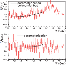
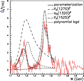
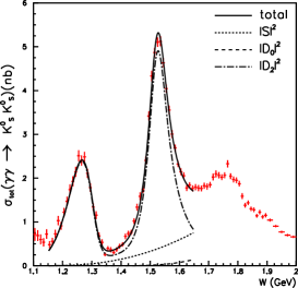
Figure 18: The solution H of the $f_{2}^{\prime}(1525)$ fit (solid line) superimposed on the spectrum of $\hat{S}^{2}$ (left top), $\hat{D}_{0}^{2}$ (left bottom), $\hat{D}_{2}^{2}$ (middle) and on the integrated cross section (for $|\cos\theta^{*}|\leq 0.8$) (right). In the $\hat{D}_{2}^{2}$ spectrum, the fitted results of the $f_{2}(1270)$ (long-dashed line), $a_{2}(1320)$ (dashed line) and $f_{2}^{\prime}(1525)$ (dot-dashed line) are also shown together with the fitted non-resonant background $|B_{D2}|^{2}$ (dotted line). In the integrated cross section, the fitted results of $|S|^{2}$ (dotted line), $|D_{0}|^{2}$ (dashed line) and $|D_{2}|^{2}$ (dot-dashed line) are also shown.

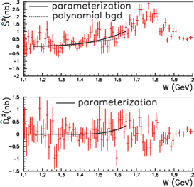
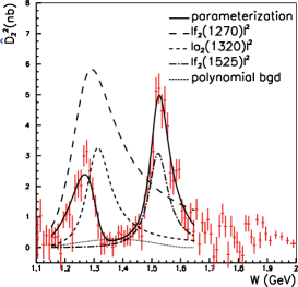
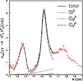
Figure 19: The solution L of the $f_{2}^{\prime}(1525)$ fit (solid line) superimposed on the spectrum of $\hat{S}^{2}$ (left top), $\hat{D}_{0}^{2}$ (left bottom), $\hat{D}_{2}^{2}$ (middle), and on the integrated cross section (for $|\cos\theta^{*}|\leq 0.8$). See the caption of Fig. 18 for the line convention (also shown in the legends).

The following sources of systematic uncertainties for the fitted parameters are considered: dependence on the fit region, normalization errors of the differential cross section, assumptions on the background amplitudes and assumed parameters of the $f_{2}(1270)$ and $a_{2}(1320)$. In each study, a fit is performed that allows all the parameters to float; the differences of the fitted parameters from the nominal values are quoted as systematic uncertainties for both solutions, H and L.

Two fitting regions shifted by $\pm 0.05$ GeV (10% of the $W$-range), are used to estimate the systematics associated with the fitting range. The systematic uncertainties associated with the normalization are separated into two groups: one from the overall normalization ($\pm 4.0$%) and the other from the distortion of the spectra in both $|\cos\theta^{*}|$ and $W$. To estimate the uncertainty associated with the overall normalization, fits are performed by shifting the cross sections coherently by $\pm 4$%. For point-by-point normalization, fits are performed by shifting the cross section by $\pm|d\sigma/d\Omega|\times\sigma_{\epsilon(W,|\cos\theta^{*}|)}$, where $\sigma_{\epsilon}$ is the relative uncertainty of the efficiency (referred to as Efficiency in Table 7). For the spectral distortion studies, the differential cross sections are shifted by $\pm 0.1\times|d\sigma/d\Omega|\times(|\cos\theta^{*}|-0.4))$ (referred to as $|\cos\theta^{*}|$ bias) and $\pm 0.08\times|d\sigma/d\Omega|\times(W-1.4~{}{\rm GeV})$ (referred to as $W$ bias). We use the absolute value of $d\sigma/d\Omega$ because some of the central values for measured differential cross sections are negative due to background subtraction.

For studies of background (BG) amplitudes, each background wave is approximated by a constant or a parabola. The value of $r_{R}$ is changed by $\pm 0.03~{}({\rm GeV}/c)^{-1}$ according to Refs. mori1 ; mori2 . Finally, the parameters of the $f_{2}(1270)$ and $a_{2}(1320)$ are changed one by one by their uncertainties shown in PDG pdg2012 .

The total systematic uncertainties are calculated by adding the individual uncertainties in quadrature. The resulting systematic uncertainties are summarized in Table 7. In some of our studies, the value of $\Gamma_{\gamma\gamma}{\cal B}(K\bar{K})$ for the $f_{2}^{\prime}(1525)$ fluctuates between the H and L solutions. The obtained results for the relative phase between the $a_{2}(1320)$ and $f_{2}(1270)$ and parameters of the $f_{2}^{\prime}(1525)$ are given in Table 6.

Table 7: Systematic uncertainties for the $f_{2}^{\prime}(1525)$ fit. The left (right) number in each row for each observable indicates a positive (negative) deviation from the nominal values.

	Solution H								Solution L
			$f_{2}^{\prime}(1525)$								$f_{2}^{\prime}(1525)$
Source	$\phi_{a2}$		Mass		$\Gamma_{\rm tot}$		$\Gamma_{\gamma\gamma}{\cal B}(K\bar{K})$		$\phi_{a2}$		Mass		$\Gamma_{\rm tot}$		$\Gamma_{\gamma\gamma}{\cal B}(K\bar{K})$
	(deg.)		(MeV/$c^{2}$)		(MeV)		(eV)		(deg.)		(MeV/$c^{2}$)		(MeV)		(eV)
$W$-range	6.1	$-0.3$	2.9	0.0	1.5	0.0	32	$0$	1.7	$-1.1$	0.7	$-0.3$	3.2	0.0	0	$-2$
$W$ bias	0.0	$-3.0$	0.0	$-0.2$	0.0	$-0.1$	2	$0$	0.3	$-0.3$	0.1	0.0	0.2	0.0	0	$0$
Efficiency	2.9	$-2.8$	0.0	$-0.2$	0.1	$-0.2$	0	$-4$	2.4	$-1.3$	0.1	$-0.1$	0.9	0.0	2	$-6$
Overall normalization	1.0	$-1.0$	0.0	$-0.1$	0.1	$-0.1$	1	$-1$	0.9	$-0.9$	0.1	$-0.1$	0.1	0.0	2	$-3$
$|\cos\theta^{*}|$ bias	0.1	$-0.1$	0.1	$-0.2$	0.7	$-0.8$	1	$-4$	0.3	$-0.2$	0.2	$-0.1$	0.8	$-0.6$	1	$-1$
$B_{S}$	0.8	$-1.8$	0.0	$-1.2$	1.1	$-1.3$	28	$-29$	1.5	$-1.2$	0.0	$-0.4$	1.9	0.0	0	$-3$
$B_{D0}$	0.0	$-3.1$	0.0	$-0.8$	0.2	$-1.9$	0	$-25$	0.0	$-0.2$	0.2	0.0	0.0	$-0.6$	0	$0$
$B_{D2}$	0.0	$-2.8$	0.0	$-1.5$	0.0	$-2.1$	0	$-21$	5.0	0.0	1.3	$-0.9$	0.6	0.0	32	$-1$
Mass($f_{2}(1270)$)	0.0	$-4.0$	0.0	$-0.3$	0.0	$-0.2$	2	$-3$	1.1	$-1.1$	0.1	0.0	0.2	0.0	1	$-1$
$\Gamma_{\rm tot}(f_{2}(1270))$	0.0	$-2.9$	0.0	$-0.1$	0.1	0.0	5	$0$	0.2	$-0.2$	0.2	$-0.1$	0.2	0.0	1	$-1$
${\cal B}(\gamma\gamma)(f_{2}(1270))$	0.0	$-4.7$	0.1	$-0.5$	0.3	$-0.4$	0	$-1$	1.8	$-1.6$	0.3	$-0.2$	1.3	0.0	3	$-4$
$r_{R}$	0.0	$-3.0$	0.0	$-0.2$	0.0	$-0.2$	1	$-1$	0.1	$-0.1$	0.1	0.0	0.0	0.0	0	$0$
Mass($a_{2}(1320)$)	0.0	$-3.8$	0.0	$-0.2$	0.0	$-0.3$	0	$-4$	0.6	$-0.8$	0.1	0.0	0.2	$-0.1$	0	$0$
$\Gamma_{\rm tot}(a_{2}(1320))$	0.0	$-5.9$	0.0	$-1.6$	0.0	$-0.8$	3	$-63$	0.2	$-0.1$	0.3	$-0.2$	0.4	$-0.1$	0	$-1$
${\cal B}(\gamma\gamma)(a_{2}(1320)$	0.0	$-3.5$	0.0	$-0.3$	0.0	0.0	6	$-2$	0.7	$-0.2$	0.1	0.0	1.1	$-0.1$	1	$-3$
Total	6.9	$-12.5$	2.9	$-2.7$	2.0	$-3.4$	43	$-77$	6.5	$-3.1$	1.6	$-1.1$	4.3	$-0.9$	33	$-10$

VI.2.4 A fit including the $f_{J}(1710)$

We fit the region $1.2~{}{\rm GeV}\leq W\leq 2.0~{}{\rm GeV}$ by fixing the parameters of the $f_{2}^{\prime}(1525)$ and $\phi_{a2}$ to either the H or L solution, and by including the contribution of the $f_{0}(1710)$ (coined the “$f_{0}(1710)$ fit”). The background amplitude is assumed to be a second-order polynomial, whose parameters are floated in the fit.

A unique solution is obtained for each of the H and L solutions (named “fit-H” and “fit-L,” where H and L stand for the H and L solutions of the $f_{2}^{\prime}(1525)$ fit, respectively). These solutions are summarized in Table 8. Figures 20 and 21 show the fitted results for fit-H and fit-L, respectively. Figures 22 and 23 show fit-H and fit-L solutions superimposed on the differential cross section for selected $W$ bins.

We also study a case where the structure near $W=1.8$ GeV is assumed to be due to a tensor meson (labeled the $f_{2}(1710)$, which can be either $a_{2}(1700)$ or $f_{2}(1810)$ (referred to as the “$f_{2}(1710)$ fit”). The contribution from tensor mesons may be suppressed due to destructive interference between the $f_{2}(1810)$ and $a_{2}(1700)$; this hypothesis could also be tested by analyzing $\gamma\gamma\to K^{+}K^{-}$ data. A unique best fit with poor $\chi^{2}$ is obtained for the $f_{2}(1710)$ fit with either of the H and L solutions of the $f_{2}^{\prime}(1525)$ fit. Thus, the hypothesis of $J=2$ for the $f_{J}(1710)$ is disfavored by the data. Fitted values are summarized in Table 8. Figures 24 and 25 show the fitted results for the $f_{2}(1710)$ fit for each of the H and L solutions.

Furthermore, we fit the hypothesis where we assume no resonance near $W=1.8$ GeV. Three best fits are obtained for the hypothesis H of the $f_{2}^{\prime}(1525)$ fit with poor $\chi^{2}/ndf$: 1264.5/589, 1265.3/589 and 1267.8/589. One best fit is obtained for the L hypothesis with even worse $\chi^{2}/ndf$ of 1349.8/589. We conclude that our fit favors the presence of the $f_{0}(1710)$ in our data.

Systematic uncertainties are estimated similarly to those for the $f_{2}^{\prime}(1525)$ fit. In the $W$-range study, fits are performed in two fit regions: $1.12~{}{\rm GeV}\leq W\leq 1.92~{}{\rm GeV}$ and $1.28~{}{\rm GeV}\leq W\leq 2.08~{}{\rm GeV}$. For $W$-distortion, a study is performed by shifting the cross section by $\pm 0.08\times|d\sigma/d\Omega|(W-1.6~{}{\rm GeV})$; for background waves, by changing each wave to a first- or third-order polynomial; and for the parameters of the $f_{2}^{\prime}(1525)$, by shifting the values by their MINOS errors. The results for the systematic uncertainties are summarized in Table 9. Table 8 lists the results for the $f_{0}(1710)$ fit (fit-H and fit-L).

Table 8: Fitted parameters for the $f_{0}(1710)$ fit and $f_{2}(1710)$ fit. For the $f_{0}(1710)$ fit, the first errors are statistical and the second systematic; they are summarized in Table 9. The parameters where the H and L solutions are combined are also shown (explained in Sec. VI.2.5).

Parameter	$f_{0}(1710)$ fit				$f_{2}(1710)$ fit
	fit-H	fit-L	H,L combined	PDG	fit-H	fit-L
$\chi^{2}/ndf$	694.2/585	701.6/585	–	–	796.3/585	831.5/585
Mass(${f_{J}})$ (MeV/$c^{2}$)	$1750^{+5+29}_{-6-18}$	$1749^{+5+31}_{-6-42}$	$1750^{+6+29}_{-7-18}$	$1720\pm 6$	$1750^{+6}_{-7}$	$1729^{+6}_{-7}$
$\Gamma_{\rm tot}({f_{J}})$ (MeV)	$138^{+12+96}_{-11-50}$	$145^{+11+31}_{-10-54}$	$139^{+11+96}_{-12-50}$	$135\pm 6$	$132^{+12}_{-11}$	$150\pm 10$
$\Gamma_{\gamma\gamma}{\cal B}(K\bar{K})_{f_{J}}$ (eV)	$12^{+3+227}_{-2-8}$	$21^{+6+38}_{-4-26}$	$12^{+3+227}_{-2-8}$	unknown	$2.1^{+0.5}_{-0.3}$	$1.6\pm 0.2$

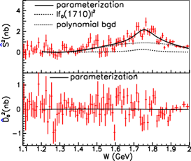
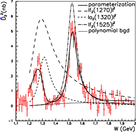
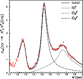
Figure 20: The fit-H of the $f_{0}(1710)$ fit (solid line) superimposed on the spectrum of $\hat{S}^{2}$ (left top), $\hat{D}_{0}^{2}$ (left bottom), $\hat{D}_{2}^{2}$ (middle) and on the integrated cross section (for $|\cos\theta^{*}|\leq 0.8$) (right). Shown in the $\hat{S}^{2}$ ($\hat{D}_{2}^{2}$) spectrum are the fitted results of the $f_{0}(1710)$ (dashed line) and non-resonant background $|B_{S}|^{2}$ (dotted line) ($f_{2}(1270)$ (long-dashed line), $a_{2}(1320)$ (dashed line), $f_{2}^{\prime}(1525)$ (dot-dashed line) and $|B_{D2}|^{2}$ (dotted line)). In the integrated cross section, the fitted results of $|S|^{2}$ (dotted line), $|D_{0}|^{2}$ (dashed line, not visible) and $|D_{2}|^{2}$ (dot-dashed line) are also shown.

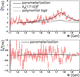
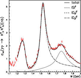
Figure 21: The fit-L of the $f_{0}(1710)$ fit (solid line) superimposed on the spectrum of $\hat{S}^{2}$ (left top), $\hat{D}_{0}^{2}$ (left bottom)), $\hat{D}_{2}^{2}$ (middle) and on the integrated cross section (for $|\cos\theta^{*}|\leq 0.8$) (right). See the caption of Fig. 20 for the line convention (also shown in the legends).

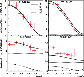
Figure 22: The fit-H of the $f_{0}(1710)$ fit (solid line) on the differential cross section for selected $W$ bins. Contributions from $|S|^{2}$ (dotted line), $|D_{0}|^{2}$ (dashed line) and $|D_{2}|^{2}$ (dot-dashed line) are also shown.

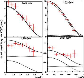
Figure 23: The fit-L of the $f_{0}(1710)$ fit (solid line) superimposed on the differential cross section for selected $W$ bins. Contributions from $|S|^{2}$ (dotted line), $|D_{0}|^{2}$ (dashed line) and $|D_{2}|^{2}$ (dot-dashed line) are also shown.

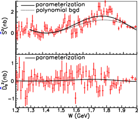
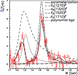
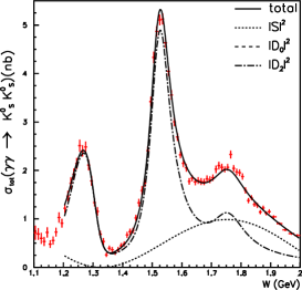
Figure 24: The fit-H for the $f_{2}(1710)$ fit (solid line) superimposed on the spectrum of $\hat{S}^{2}$ (left top), $\hat{D}_{0}^{2}$ (left bottom), $\hat{D}_{2}^{2}$ (middle) and integrated cross section (for $|\cos\theta^{*}|\leq 0.8$) (right). Shown in the $\hat{D}_{2}^{2}$ ($\hat{S}^{2}$) spectrum are the fitted results $f_{2}(1270)$ (long-dashed line), $a_{2}(1320)$ (dashed line), $f_{2}^{\prime}(1525)$ (dot-dashed line), $f_{2}(1710)$ (very-long-dashed line) and non-resonant background $|B_{D2}|^{2}$ (dotted line) ($|B_{S}|^{2}$ (dotted line)). In the integrated cross section, the fitted results of $|S|^{2}$ (dotted line), $|D_{0}|^{2}$ (dashed line) and $|D_{2}|^{2}$ (dot-dashed line) are also shown.

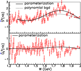
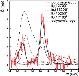
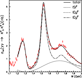
Figure 25: The fit-L for the $f_{2}(1710)$ fit (solid line) superimposed on the spectrum of $\hat{S}^{2}$ (left top), $\hat{D}_{0}^{2}$ (left bottom), $\hat{D}_{2}^{2}$ (middle) and integrated cross section (for $|\cos\theta^{*}|\leq 0.8$) (right). See the caption of Fig. 24 for the line convention (also shown on plots).

Table 9: Systematic uncertainties for the $f_{0}(1710)$ fit. The left (right) number in each row for each observable indicates a positive (negative) deviation from the nominal values.

	Fit-H						Fit-L
Source	Mass		$\Gamma_{\rm tot}$		$\Gamma_{\gamma\gamma}{\cal B}(K\bar{K})$		Mass		$\Gamma_{\rm tot}$		$\Gamma_{\gamma\gamma}{\cal B}(K\bar{K})$
	(MeV/$c^{2}$)		(MeV)		(eV)		(MeV/$c^{2}$)		(MeV)		(eV)
$W$-range	21	0	0	$-15$	0	$-1$	16	0	5	$-13$	6	$-4$
$W$ bias	2	$-2$	6	$-5$	2	$-1$	4	0	2	$-7$	2	$-4$
Efficiency	8	$-4$	25	$-30$	209	0	11	$-5$	0	$-28$	2	$-12$
Overall normalization	4	$-2$	9	$-11$	1	$-2$	7	$-2$	4	$-16$	5	$-8$
$|\cos\theta^{*}|$ bias	0	$-1$	3	$-1$	1	0	4	0	2	$-7$	2	$-4$
$B_{S}$	5	$-7$	84	$-9$	87	$-2$	7	0	26	$-3$	35	$-2$
$B_{D0}$	0	0	1	0	0	0	1	0	0	$-2$	0	$-1$
$B_{D2}$	1	0	0	$-1$	0	0	11	$-37$	4	$-11$	1	$-2$
Mass($f_{2}(1270)$)	3	$-1$	6	$-6$	1	$-1$	3	0	0	$-4$	2	$-3$
$\Gamma_{\rm tot}(f_{2}(1270))$	0	0	1	0	0	0	2	$-2$	5	$-4$	4	$-2$
${\cal B}(\gamma\gamma)(f_{2}(1270))$	7	0	12	$-18$	2	$-4$	6	$-1$	0	$-17$	5	$-10$
$r_{R}$	0	0	0	0	0	0	1	$-1$	1	0	1	0
Mass($a_{2}(1320)$)	1	0	0	$-2$	0	0	2	0	0	$-2$	0	$-1$
$\Gamma_{\rm tot}(a_{2}(1320))$	2	$-2$	7	$-5$	2	$-1$	3	0	2	$-9$	3	$-6$
${\cal B}(\gamma\gamma)(a_{2}(1320))$	1	$-1$	2	0	1	0	2	0	0	$-2$	0	$-1$
Mass($f_{2}^{\prime}(1525)$)	2	$-2$	1	0	1	0	1	$-1$	3	$-4$	3	$-3$
$\Gamma_{\rm tot}(f_{2}^{\prime}(1525))$	2	$-2$	4	$-3$	2	$-1$	4	0	0	$-4$	0	$-2$
${\cal B}(\gamma\gamma)(f_{2}^{\prime}(1525))$	14	0	0	$-24$	0	$-4$	14	$-18$	14	$-27$	9	$-12$
$\phi_{f_{2}^{\prime}(1525)}$	4	$-15$	33	$-12$	22	$-3$	4	$-5$	0	$-17$	3	$-11$
$\phi_{a_{2}(1320)}$	4	$-1$	5	$-8$	1	$-2$	3	0	0	$-4$	0	$-2$
Total	29	$-18$	96	$-50$	227	$-8$	31	$-42$	31	$-54$	38	$-26$

VI.2.5 Final results for the region $W<2.0~{}{\rm GeV}$

As described above, we obtain two solutions referred to as H and L for the $f_{2}^{\prime}(1525)$ fit, and corresponding fits are performed in the $f_{0}(1710)$ fit by fixing the $f_{2}^{\prime}(1525)$ parameters to those of either the H or L solution. Here, we combine solutions statistically to obtain final results.

From each pair of solutions for an observable $x$, a probability density function (PDF) $P(x)$ is formed as the sum of asymmetric Gaussian functions that correspond to the two solutions with asymmetric errors. These functions are weighted according to the $\chi^{2}$ differences between the two solutions. The most probable value $x_{f}$ is the one that gives the maximum in $P(x)$. Asymmetric statistical errors $\sigma^{l}$ and $\sigma^{h}$ are determined from a confidence interval such that $P(x_{f}-\sigma^{l})=P(x_{f}+\sigma^{h})$ with

$$\int_{x_{f}-\sigma^{l}}^{x_{f}+\sigma^{h}}P(x)dx=0.683\;.$$ (17)

The systematic uncertainty for observable $x$ is determined from the solution with the largest deviation from $x_{f}$. The final results thus obtained are listed in Tables 6 and 8.

VI.3 Fitting the region $W>2.0$ GeV

We investigate the structures around 2.3 and 2.6 GeV. In fitting the region $2.0~{}{\rm GeV}\leq W\leq 3.0~{}{\rm GeV}$, we assume that the non-resonant backgrounds in the S, D₀, D₂, G₀ and G₂ waves obey a power law in $W$. When we parameterize them using a polynomial approximation as in Eq. (10), we obtain fits of poor quality. We parameterize the backgrounds as

$$B_{i}=b_{i}\times\left(\frac{W}{W_{0}}\right)^{-c_{i}}e^{i\phi_{i}},$$ (18)

where the index $i$ denotes S, D₀, D₂, G₀ or G₂ waves, $W_{0}$ is chosen to be the lower boundary of the fitting region (nominally $W_{0}=2.0$ GeV), and $b_{i}$ and $c_{i}$ are the free parameters. The phases of $B_{S}$ and $B_{D2}$ are chosen to be zero as a reference for the other phases. The parameters $b_{i}$ are set positive to resolve arbitrary sign ambiguities.

We also investigate a possible contribution from the $J=4$ resonances. Table 10 summarizes the parameters of the $f_{0}(2200)$, $f_{2}(2300)$ and $f_{4}(2300)$ that are known to couple to $K\bar{K}$ pdg2012 .

We allow $B_{G0}$ and/or $B_{G2}$ to be non-zero in Eq. (18). We fit 13 assumptions for the structures around 2.3 and 2.6 GeV that are observed in the plot of the integrated cross section shown in Fig. 12(a). A fit performed assuming the presence of the $f_{J}(2200)$ ($J=0,2,4$) and $f_{J^{\prime}}(2500)$ ($J^{\prime}=0,2,4$) is referred to as an “$f_{J}$-$f_{J^{\prime}}$ fit.” We also investigate hypotheses in which there are no resonances (or only one) for the two structures. These fits are referred to as “no-resonance-” (“only-$f_{J}$-”) fits, respectively.

When both $B_{G0}$ and $B_{G2}$ are allowed to be non-zero, too many solutions are obtained because of the several combinations of interfering amplitudes (not shown). Thus, we focus on the hypothesis wherein only $B_{G2}$ is non-zero. This choice is based on the idea that the possible resonances $f_{4}(2200)$ and $f_{4}(2500)$ are included in the G₂ wave only because of helicity considerations. A summary of the fitted results is given in Table 11. In this case, once again, some of the $f_{J}$-$f_{J^{\prime}}$ fits give multiple solutions. In some cases, one or more $c_{i}$ values in Eq. (18) assume unphysically large values. Thus, we constrain the maximum values of $c_{i}$ to be 20.

A unique solution of relatively good quality is obtained for the $f_{2}$-$f_{0}$ fit, while other hypotheses yield larger values of $\chi^{2}/ndf$. The $f_{2}$-$f_{0}$ fit is also favored for the case in which both $B_{G0}$ and $B_{G2}$ are assumed to be non-zero. Thus, we conclude that the structure around 2.3 GeV is likely due to a tensor meson (referred to tentatively as $f_{2}(2200)$) and the one near 2.6 GeV is likely to be a scalar meson (possibly $f_{0}(2500)$).

The fitted values obtained from the $f_{2}$-$f_{0}$ fit are summarized in Table 12 for the mass, total width and $\Gamma_{\gamma\gamma}{\cal B}(K\bar{K})$ of the $f_{2}(2200)$ and $f_{0}(2500)$. Figure 26 shows the fitted results for the $f_{2}$-$f_{0}$ fit superimposed on the integrated cross section. Figure 27 shows the fitted results and contributions of $|S|^{2}$, $|D_{0}|^{2}$, $|D_{2}|^{2}$, and $|G_{2}|^{2}$ to the differential cross section in selected $W$ bins. The systematic uncertainties shown in Table 12 are estimated similarly to those described in Sec. VI.2. To estimate the uncertainties from the background parameterization, the background amplitudes are changed to $b_{i}((W\pm 1~{}{\rm GeV})/W_{0})^{-c_{i}}$. The results of the studies of systematic uncertainties are summarized in Table 13.

Table 10: Parameters of the $f_{0}(2200)$, $f_{2}(2300)$ and $f_{4}(2300)$ pdg2012 .

Parameter	$f_{0}(2200)$	$f_{2}(2300)$	$f_{4}(2300)$
Mass (MeV/$c^{2}$ )	$2189\pm 13$	$2297\pm 28$	$\sim 2300$
$\Gamma_{\rm tot}$ (MeV)	$238\pm 50$	$149\pm 41$	$250\pm 80$
$f_{J}\to K\bar{K}$	seen	seen	seen
$f_{J}\to\gamma\gamma$	unknown	seen	unknown

Table 11: Summary of fitted results for $2.0~{}{\rm GeV}\leq W\leq 3.0~{}{\rm GeV}$ for 13 assumptions (with G₂ background).

Assumption	No. of sol.	$\chi^{2}$	$ndf$
$f_{0}$-$f_{0}$	2	293.3, 293.9	214
$f_{0}$-$f_{2}$	4	320.9, 321.9, 324.5, 327.6	214
$f_{0}$-$f_{4}$	1	291.4	214
$f_{2}$-$f_{0}$	1	228.3	214
$f_{2}$-$f_{2}$	1	260.4	214
$f_{2}$-$f_{4}$	1	323.6, 306.7	214
$f_{4}$-$f_{0}$	1	411.6	214
$f_{4}$-$f_{2}$	2	468.6, 472.1	214
$f_{4}$-$f_{4}$	4	459.6, 464.1, 466.4, 467.5	214
Only-$f_{0}$	1	390.0	218
Only-$f_{2}$	1	323.6	218
Only-$f_{4}$	1	518.7	218
No resonances	1	659.32	222

Table 12: Parameters obtained from the $f_{2}$-$f_{0}$ fit. The first errors are statistical and the second systematic (summarized in Table 13).

Parameter	$f_{2}(2200)$	$f_{0}(2500)$
Mass (MeV/$c^{2}$)	$2243^{+7+3}_{-6-29}$	$2539\pm 14{}^{+38}_{-14}$
$\Gamma_{\rm tot}$ (MeV)	$145\pm 12{}^{+27}_{-34}$	$274^{+77+126}_{-61-163}$
$\Gamma_{\gamma\gamma}{\cal B}(K\bar{K})$ (eV)	$3.2^{+0.5+1.3}_{-0.4-2.2}$	$40^{+9+17}_{-7-40}$

Table 13: Systematic uncertainties for the $f_{2}$-$f_{0}$ fit. The left (right) number in each row for each observable indicates a positive (negative) deviation from the nominal values.

	$f_{0}(2200)$						$f_{0}(2500)$
Source	Mass		$\Gamma_{\rm tot}$		$\Gamma_{\gamma\gamma}{\cal B}(K\bar{K})$		Mass		$\Gamma_{\rm tot}$		$\Gamma_{\gamma\gamma}{\cal B}(K\bar{K})$
	(MeV/$c^{2}$)		(MeV)		(eV)		(MeV/$c^{2}$)		(MeV)		(eV)
$W$-range	3	$-3$	26	$-14$	1.3	$-0.7$	6	$-11$	101	$-89$	10	$-5$
$W$ bias	0	$0$	0	$0$	0.1	$-0.1$	0	$0$	8	$-7$	1	$-1$
Efficiency	0	$0$	1	$-1$	0.3	$-0.3$	0	$0$	9	$-9$	4	$-4$
Overall normalization	0	$0$	0	$0$	0.1	$-0.1$	0	$0$	0	$-1$	2	$-2$
$|\cos\theta^{*}|$ bias	0	$0$	0	$0$	0.1	$-0.1$	0	$0$	0	$-2$	2	$-2$
$B_{S}$	0	$-15$	0	$-24$	0.0	$-1.6$	25	$-1$	0	$-105$	0	$-39$
$B_{D0}$	0	$-15$	0	$-25$	0.0	$-1.5$	24	$0$	0	$-108$	0	$-39$
$B_{D2}$	0	$0$	0	$0$	0.0	$0.0$	0	$0$	0	$0$	0	$0$
$B_{G0}$	0	$-19$	7	$0$	0.1	$0.0$	0	$-9$	0	$-62$	0	$-3$
$B_{G2}$	0	$-1$	0	$0$	0.0	$0.0$	1	$0$	0	$-4$	0	$-1$
Total	3	$-29$	27	$-37$	1.3	$-2.3$	35	$-14$	101	$-186$	11	$-56$

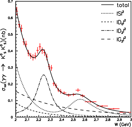
Figure 26: Result of the $f_{2}$-$f_{0}$ fit (solid line) superimposed on the integrated cross section (for $|\cos\theta^{*}|\leq 0.8$). The fitted results of $|S|^{2}$ (dotted line), $|D_{0}|^{2}$ (dashed line), $|D_{2}|^{2}$ (dot-dashed line) and $|G_{2}|^{2}$ (long-dashed line) are also shown.

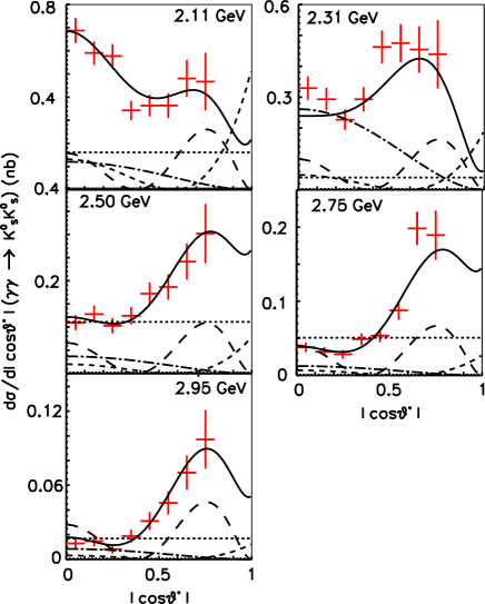
Figure 27: Differential cross section and the fitted results of the $f_{2}$-$f_{0}$ fit (solid line) at the $W$ bins indicated in each panel. The contributions of $|S|^{2}$ (dotted line), $|D_{0}|^{2}$ (dashed line), $|D_{2}|^{2}$ (dot-dashed line) and $|G_{2}|^{2}$ (long-dashed line) are also shown.

VI.4 Discussion of the results of the resonance study

In this subsection, we summarize the fitted results and discuss their implications. First, the destructive interference between the $f_{2}(1270)$ and $a_{2}(1320)$ lipkin is confirmed with high accuracy; the relative phase, $\phi_{a2}$, is measured to be $\left(172.6^{+6.0+12.2}_{-0.7-7.0}\right)^{\circ}$, where the first error is statistical and the second systematic. The mass, total width and $\Gamma_{\gamma\gamma}{\cal B}(K\bar{K})$ of the $f_{2}^{\prime}(1525)$ are measured to be $1525.3^{+1.2+3.7}_{-1.4-2.1}~{}{\rm MeV}/c^{2}$, $82.9^{+2.1+3.3}_{-2.2-2.0}~{}{\rm MeV}$ and $48^{+67}_{-8}{}^{+108}_{-12}~{}{\rm eV}$, respectively. The systematic uncertainty of $\Gamma_{\gamma\gamma}{\cal B}(K\bar{K})$ is fairly large. Nevertheless, this is the first measurement of this parameter that includes the interference with a non-resonant amplitude.

The structure near 1.6 GeV is attributed to a scalar meson and is interpreted to be the $f_{0}(1710)$. To obtain the significance for the assignment of the $f_{0}(1710)$ over that of the $f_{2}(1710)$, fits are performed for each of the sources of systematic uncertainty for the two hypotheses and the minimum $\chi^{2}$ difference is identified among these fits. It is found to be 63.3, which corresponds to a significance of 7.9$\sigma$ favoring the $f_{0}(1710)$.

A similar study is performed for the $f_{J}(2200)$ hypothesis by comparing the values of $\chi^{2}_{\rm min}$ of the $f_{2}$-$f_{0}$ fit and $f_{0}$-$f_{0}$ fit for each source of systematic uncertainty. We obtain a minimum $\chi^{2}$ difference to be of 11.3, corresponding to a $3.4\sigma$ significance. For the $f_{0}(2500)$, the $f_{2}$-$f_{0}$ fit gives the best $\chi^{2}$; the next best, the $f_{2}$-$f_{2}$ fit, yields a $4.3\sigma$ significance. Thus, while we cannot make definitive assignments about the spins of the $f_{J}(2200)$ and $f_{J^{\prime}}(2500)$, $J=2$ and $J^{\prime}=0$ hypotheses, respectively, are favored.

The values of $\Gamma_{\gamma\gamma}{\cal B}(K\bar{K})$ for the $f_{0}(1710)$, $f_{2}(2200)$ and $f_{0}(2500)$ are estimated for the first time and are found to be $12^{+3+227}_{-2-8}~{}{\rm eV}$, $3.2^{+0.5+1.3}_{-0.4-2.2}~{}{\rm eV}$ and $40^{+9+17}_{-7-40}~{}{\rm eV}$, respectively. Each value could provide important information on the constituents of the corresponding resonance. For example, the $f_{0}(1710)$ is identified as an unmixed scalar glueball according to a coupled-multi-channel analysis albaladejo . However, the $f_{0}(1710)$ is unlikely to be a glueball candidate because the observed value of $\Gamma_{\gamma\gamma}{\cal B}(K\bar{K})$, combined with the implied value of $\Gamma_{\gamma\gamma}{\cal B}(\pi\pi)$ ($\simeq\Gamma_{\gamma\gamma}{\cal B}(K\bar{K})$ for the flavor-SU(3)-symmetric decay of a glueball) would indicate a large two-photon width, contrary to the expectation of much less than 1 eV for a glueball (see, e.g., Refs. scalar ; scalar2 ; scalar3 ; scalar4 ). Therefore, we conclude that the $f_{0}(1710)$ is a resonance with a large $s\bar{s}$ admixture.

The measured mass of the $f_{2}(2200)$, $2243^{+7+3}_{-6-29}~{}{\rm MeV}/c^{2}$, is close to that of the $f_{J}(2220)$ and smaller than that of the $f_{2}(2300)$ pdg2012 . The $f_{J}(2220)$ is usually assumed to be a glueball candidate due to the small value of its total width ($23^{+8}_{-7}~{}{\rm MeV}$). The structure found by Belle in the $\gamma\gamma\to K^{+}K^{-}$ reaction around 2.3 GeV kabe is interpreted as the $f_{2}(2300)$ by PDG pdg2012 . The measured total width of the $f_{2}(2200)$, $145\pm 12{}^{+27}_{-34}$ MeV, is much wider than that of the $f_{J}(2220)$ and is similar to that of the $f_{2}(2300)$.

The $f_{0}(2500)$, whose mass and width are found to be $2539\pm 14{}^{+38}_{-14}~{}{\rm MeV}/c^{2}$ and $274^{+77+126}_{-61-163}~{}{\rm MeV}$, respectively, is the first scalar to be identified in this mass region pdg2012 ; this observation invites an independent confirmation.

VII Derivation of charmonium contribution

We present our estimates of the $\chi_{c0}$ and $\chi_{c2}$ contributions by measuring the yields of the fit components in the region $|\cos\theta^{*}|<0.5$ and $2.8~{}{\rm GeV}<W<4.0$ GeV (Fig. 28). We use only samples with $|\cos\theta^{*}|<0.5$ to enhance the fraction of the charmonium components while disentangling them from the continuum contribution. We derive $\Gamma_{\gamma\gamma}(R){\cal B}(R\to K^{0}_{S}K^{0}_{S})$ for these charmonium states. We also search for a possible contribution from a higher-mass charmonium in the 3.6 – 4.0  GeV/$c^{2}$ region.

We assume the angular distributions for the $\chi_{c0}$ and $\chi_{c2}$ components to be flat and proportional to $\sin^{4}\theta^{*}$ (from pure helicity-2 kabe2 ), respectively, to derive $\Gamma_{\gamma\gamma}{\cal B}$ from the yield in $|\cos\theta^{*}|<0.5$. We discuss the effect of interference with the continuum.

VII.1 Evaluation of parameters for the $\chi_{cJ}$ charmonia

The peak structures observed in the yield distribution for $3.3~{}{\rm GeV}<W<3.6~{}{\rm GeV}$ (Fig. 28) are from charmonium production: $\gamma\gamma\to\chi_{c0}$, $\chi_{c2}\to K^{0}_{S}K^{0}_{S}$. We fit the distribution to contributions from the $\chi_{c0}$ and $\chi_{c2}$ as well as a smooth continuum component represented by

$$Y(W) = |\sqrt{\alpha kW^{-\beta}}+e^{i\phi}\sqrt{N_{\chi_{c0}}}{\rm BW}_{\chi_{c0}}(W)|^{2}+$$ (19)

$$N_{\chi_{c2}}|{\rm BW}_{\chi_{c2}}(W)|^{2}+\alpha(1-k)W^{-\beta},$$

in the $W$ and $|\cos\theta^{*}|$ ranges 2.9 – 3.7 GeV and $|\cos\theta^{*}|<0.5$, respectively, where ${\rm BW}_{\chi_{cJ}}(W)$ is a Breit-Wigner function for the charmonium amplitude, which is proportional to $1/(W^{2}-M_{\chi_{cJ}}^{2}-iM_{\chi_{cJ}}\Gamma_{\chi_{cJ}})$ and is normalized by $\int|{\rm BW}_{\chi_{cJ}}(W)|^{2}dW=1$. The component $\alpha W^{-\beta}$ corresponds to the contribution from the continuum, with a fraction $k$ that interferes with the $\chi_{c0}$ amplitude with a relative phase $\phi$.

It is impossible to determine the interference parameters for the $\chi_{c2}$ by any fits because of its smaller intrinsic width compared to the mass resolution. We fit the $\chi_{c2}$ yield ($N_{\chi_{c2}}$) with a function in which no interference term is included, as shown by Eq. (19); later, we estimate the maximum effects from the interference term when we evaluate the uncertainty for the two-photon decay width of $\chi_{c2}$.

All parameters except the width of the $\chi_{c2}$ are free. The $\chi_{c2}$ width is fixed to 2.0 MeV, which is smaller than the estimated mass resolution of $\sim 7$ MeV. Smearing effects due to a non-zero mass resolution are taken into account in the fit, using a Gaussian function with $\sigma=7.0$ MeV. The small $W$ dependence of the product of the efficiency and luminosity function, $\mp 0.95\%$ for a change in $W$ of $\pm 10$ MeV, is folded in the $\chi_{c0}$ resonance curve.

A binned maximum likelihood method is applied with the bin width $\Delta W=10$ MeV. We examine two cases: with and without the interference of the $\chi_{c0}$. We could not determine the $k$ parameter; that is, any $0<k\leq 1$ gives exactly the same fit quality for the constructive ($\phi\approx\pi/2$) and destructive ($\phi\approx 3\pi/2$) interference cases. Therefore, the statistical error range for the yield of $\chi_{c0}$ corresponds to the full range of the interference assumption $0<k\leq 1$.

The maximum effect of the interference of $\chi_{c2}$ with the continuum component is calculated from Eq. (20) because we cannot measure it from the line shape of the charmonium, so we include its maximum possible range in the statistical error. The number of $\chi_{c2}$ events that is proportional to the square of the resonance amplitude is converted from the observed number $N_{\chi_{c2}}$ to that with the maximum interference effect $N^{\prime}_{\chi_{c2}}$ using the relation

$$\sqrt{N^{\prime}_{\chi_{c2}}}=\sqrt{\frac{\pi\Gamma n_{I}}{2}+N_{\chi_{c2}}}\pm\sqrt{\frac{\pi\Gamma n_{I}}{2}},$$ (20)

where $\Gamma$ and $n_{I}$ are the total width of the $\chi_{c2}$ and the observed yield density of the continuum component per unit energy in the $W$ range around the $\chi_{c2}$, respectively.

The fitted results are summarized in Table 14, where ${\cal L}$ is the likelihood value. The normalization $N_{\chi_{c0}}$ in Eq. (19) is proportional to the square of the resonance amplitude, even when the interference is assumed. The yields from the fits are translated to products of the two-photon decay width and the branching fraction, $\Gamma_{\gamma\gamma}(\chi_{cJ}){\cal B}(\chi_{cJ}\to K^{0}_{S}K^{0}_{S})$, shown in Table 15.

To estimate the systematic uncertainties associated with the choice of the signal shape approximation, we vary their shape parameters. We change the $W$ resolution from 7 to 8 MeV and modify the term in the denominator of the Breit-Wigner function, from $-iM\Gamma$ to $-iW\Gamma$. The observed changes of the central values of the $\chi_{c0}$ and $\chi_{c2}$ yields are less than 3%. This is because the $\chi_{c0}$ and $\chi_{c2}$ contributions are well separated from each other, and the continuum contribution is very small around the charmonium peaks. The systematic uncertainty is thus dominated by the contributions from the efficiency and luminosity function, and is about 10% in total. The systematic uncertainties for $\Gamma_{\gamma\gamma}{\cal B}$ are shown in Table 15.

The present results are consistent with and supersede those from the previous measurements chen ; pdg2012 . The interference effect was not taken into account in the previous Belle result.

Table 14: Results of the fits (see the text) to obtain the charmonium contributions with and without interference effects. Errors are statistical only. Logarithmic likelihood ($\ln{\cal L}$) values are only meaningful when comparing two or more fits.

Interference	$N_{\chi_{c0}}$	$k$	$\phi$	$N_{\chi_{c2}}$	$-2\ln{\cal L}/ndf$
Not included	$248.3^{+17.9}_{-17.2}$	(0.0, by def.)	$-$	$53.0^{+8.1}_{-7.4}$	$57.34/73$
Included	$266\pm 53$	any of 0–1	two sols.	$53^{+14}_{-12}$	$57.22/71$

Table 15: Products of the two-photon decay width and the branching fraction for the two charmonia, where $\Gamma_{\gamma\gamma}{\cal B}(\chi_{cJ})$ is the abbreviation for $\Gamma_{\gamma\gamma}(\chi_{cJ}){\cal B}(\chi_{cJ}\to K^{0}_{S}K^{0}_{S})$. Mass and width parameters determined by the present fits are also presented. Comparisons with the previous Belle results chen and the PDG2012 pdg2012 values are also shown. The first and second errors (if given) are statistical and systematic, respectively.

Interference	$\Gamma_{\gamma\gamma}{\cal B}(\chi_{c0})$	$\Gamma_{\gamma\gamma}{\cal B}(\chi_{c2})$	Mass($\chi_{c0})$	Width($\chi_{c0}$)	Mass($\chi_{c2})$	Width($\chi_{c2})$
	(eV)	(eV)	(MeV/$c^{2}$)	(MeV)	(MeV/$c^{2}$)	(MeV)
Not included	$8.09\pm 0.58\pm 0.83$	$0.268^{+0.041}_{-0.037}\pm 0.028$	$3414.8\pm 0.9$	$13.2\pm 2.1$	$3555.4\pm 1.3$	(2.0, fix)
Included	$8.7\pm 1.7\pm 0.9$	$0.27^{+0.07}_{-0.06}\pm 0.03$	$3414.6\pm 1.1$	$13.2\pm 2.1$	$3555.4\pm 1.3$	(2.0, fix)
Belle 2007	$7.00\pm 0.65\pm 0.71$	$0.31\pm 0.05\pm 0.03$	-	-	-	-
PDG 2012	$7.3\pm 0.5$	$0.297\pm 0.026$	$3414.75\pm 0.31$	$10.4\pm 0.6$	$3556.20\pm 0.09$	$1.98\pm 0.11$

Figure 28: $W$ distribution of the candidate events for $2.8~{}{\rm GeV}<W<4.0~{}{\rm GeV}$ and $|\cos\theta^{*}|<0.5$. The two distinct peaks are from the $\chi_{c0}$ and $\chi_{c2}$. The curve is a fit without interference.

VII.2 Possible higher-mass charmonium states

We could expect a contribution from the possible higher-mass charmonium states, $\chi_{cJ}(2P)$ ($J=0$, 2) in the $W$ region above 3.8 GeV. The $\chi_{c2}(2P)$ has been found near 3927 MeV/$c^{2}$ in the two-photon process pdg2012 in its decay to the $D\bar{D}$ state, but the $\chi_{c0}(2P)$ has not yet been observed in this decay mode. Although no theoretical predictions are available for the branching fractions ${\cal B}(\chi_{cJ}(2P)\to K^{0}_{S}K^{0}_{S})$, a yield of a few events is expected if $\Gamma(\chi_{cJ}(2P)\to K^{0}_{S}K^{0}_{S})\approx\Gamma(\chi_{cJ}(1P)\to K^{0}_{S}K^{0}_{S})$ and postulated or observed values for $\Gamma_{\rm tot}$ and $\Gamma_{\gamma\gamma}$ for such states are taken.

As seen in Fig. 28, we find 8 events in the $W$ region between 3.7 and 4.0 GeV, consistent with 5.2 events expected in the region from the extrapolated continuum background determined by the fit below 3.7 GeV (with a continuum yield density of $dY/dW=59.2(W/3.5{\rm GeV})^{-13.5}~{}[{\rm GeV}^{-1}]$, including interference). In the $W$ region between 3.80 and 3.95 GeV, where we expect the presence of contributions from the two higher-mass charmonium states, 7 events are observed, while only 2.3 events are expected from the continuum. The probability for this observation ($p$-value) is 0.9%.

We evaluate an upper limit for $\Gamma_{\gamma\gamma}(\chi_{c2}(2P)){\cal B}(\chi_{c2}(2P)\to K^{0}_{S}K^{0}_{S})$. We find 2 events in the $\chi_{c2}(2P)$ mass region, 3.879 – 3.975 GeV/$c^{2}$, which is defined by $M\pm 2\Gamma$ using the known mass and total width pdg2012 . We adopt $N^{UL}_{\chi_{c2}(2P)}=5.32$ as the upper limit of the yield with a 90% confidence level (CL) for the contribution of the $\chi_{c2}(2P)$, assuming no background contribution for a conservative limit and based on the Poisson distribution with this mean value giving a 10% probability for two or fewer observed events. This translates into an upper limit for the product of the two-photon decay width and the branching fraction of the $\chi_{c2}(2P)$ of $\Gamma_{\gamma\gamma}(\chi_{c2}(2P)){\cal B}(\chi_{c2}(2P)\to K^{0}_{S}K^{0}_{S})<0.064~{}{\rm eV\ (90\%\ CL)}$ without interference. This upper limit takes into account the uncertainty of the efficiency by increasing the limit by one standard deviation.

The $X(3915)$ found in the $\gamma\gamma\to X(3915)\to\omega J/\psi$ process x3915be has been confirmed and its spin-parity is assigned to be $J^{P}=0^{+}$ x3915ba . Assigning this resonance to be the $\chi_{c0}(2P)$ state together with the values of mass and total width given by the most recent tabulation by PDG pdg2013 ($M=3918.4\pm 1.9$ MeV/$c^{2}$ and $\Gamma=20\pm 5$ MeV), we extract the upper limit of $\Gamma_{\gamma\gamma}(\chi_{c0}(2P)){\cal B}(\chi_{c0}(2P)\to K^{0}_{S}K^{0}_{S})<0.49~{}{\rm eV\ (90\%\ CL)}$; the same two events that are found for the analysis of the $\chi_{c2}(2P)$ in the $M\pm 2\Gamma$ region correspond to $N^{UL}_{\chi_{c0}(2P)}=5.32$.

VII.3 Search for the decay $\eta_{c}\to K^{0}_{S}K^{0}_{S}$

The decay $\eta_{c}\to K^{0}_{S}K^{0}_{S}$ violates both $P$ and $CP$ invariance. We search for this decay mode in the present data. Copious production of the $\eta_{c}$ in two-photon collisions has been established in several decay modes by previous measurements pdg2012 .

A small peak-like structure near 2.99 GeV seen in Fig. 28 is not statistically significant and corresponds to a fluctuation at the $1.7\sigma$ level, which is evaluated from the difference between log-likelihoods for the fits without and with a contribution of the $\eta_{c}$, taking into account the interference effect that is described below. We thus set the upper limit of the branching fraction for this decay mode.

We fit the event distribution in the range 2.8 GeV$<W<3.3$ GeV with a function similar to Eq. (19) in which the $\chi_{c0}$ contribution is replaced by that of the $\eta_{c}$ and the $\chi_{c2}$ term is not included. We fix the mass and width of the $\eta_{c}$ to be 2981 MeV/$c^{2}$ and 30 MeV, respectively. The best fit without interference gives $N_{\eta_{c}}=5.4\pm 5.0$. This is consistent with zero. We determine the 90% CL upper limit with the $N_{\eta_{c}}^{\rm UL}$ value that corresponds to the $(1.64)^{2}$ worse log-likelihood $-2\ln{\cal L}$ than that of the best fit.

We take into account uncertainties in the mass, width and the mass resolution associated with our measurement, and repeat the fit by adjusting these parameters by $\pm 2$ MeV/$c^{2}$, $\pm 4$ MeV and in $5--7$ MeV, respectively, and choose the most conservative upper limit. The obtained upper limit is $N_{\eta_{c}}^{\rm UL}=15$ ($N_{\eta_{c}}^{\rm UL}=85$) without (with) interference. The curves describing the results of the fits used to estimate the upper limits as described are shown in Fig. 29.

The 90% CL upper limits for $\Gamma_{\gamma\gamma}(\eta_{c}){\cal B}(\eta_{c}\to K^{0}_{S}K^{0}_{S})$ and ${\cal B}(\eta_{c}\to K^{0}_{S}K^{0}_{S})$ are summarized in Table 16; for the latter, $\Gamma_{\gamma\gamma}(\eta_{c})=5.3\pm 0.5$ keV is used pdg2012 . These upper limits take into account the uncertainties from systematic error of the measurement and the $\Gamma_{\gamma\gamma}(\eta_{c})$ value by shifting the limits by a ratio corresponding to $1\sigma$ in the direction of increased values.

Table 16: Upper limits for products of the two-photon decay width and the branching fraction for the $\eta_{c}\to K^{0}_{S}K^{0}_{S}$ decay, where $\Gamma_{\gamma\gamma}{\cal B}(\eta_{c})$ stands for $\Gamma_{\gamma\gamma}(\eta_{c}){\cal B}(\eta_{c}\to K^{0}_{S}K^{0}_{S})$.

Interference	$\Gamma_{\gamma\gamma}{\cal B}(\eta_{c})$	${\cal B}(\eta_{c}\to K^{0}_{S}K^{0}_{S})$
Not included	< 0.29 eV	< $5.6\times 10^{-5}$	90% CL
Included	< 1.6 eV	< $3.2\times 10^{-4}$	90% CL

Figure 29: Experimental event distribution in the range $2.8~{}{\rm GeV}<W<3.3~{}{\rm GeV}$ and $|\cos\theta^{*}|<0.5$ and the results of the fits used to estimate the upper limits for $\eta_{c}\to K^{0}_{S}K^{0}_{S}$ in cases with (dashed) and without (solid) interference.

VIII QCD studies in the high-energy region

In this section, the cross-section behavior is studied and compared with predictions from QCD-based models and calculations in the region $W>2.6~{}{\rm GeV}$. First, we compare the differential cross section with the $1/\sin^{4}\theta^{*}$ dependence. Then the $W^{-n}$ behavior of the integrated cross section is examined.

VIII.1 Angular dependence of the differential cross section

We compare the angular dependence of the differential cross section with the $1/\sin^{4}\theta^{*}$ dependence, which is claimed by the handbag model handbag . Earlier Belle measurements for this process supported such a dependence in the $W$ region between 2.4 and 3.3 GeV for $|\cos\theta^{*}|<0.6$ chen .

To make a quantitative statement about the behavior of the cross section, we fit the differential cross section using the approximation $A/\sin^{\alpha}\theta^{*}$, i.e.,

$$\frac{d\sigma}{d|\cos\theta^{*}|}=\frac{A}{\sin^{\alpha}\theta^{*}}$$ (21)

in each $W$ bin. We summarize the fitted results for the 12 regions in Fig. 30, where the right scales are differential cross sections normalized to the integrated cross section in the range $|\cos\theta^{*}|<0.8$ (that gives the average 1/0.8 = 1.25). This scale is added to improve the visibility of the plots for different $W$ bins. The $\chi^{2}/ndf$ values obtained from the fits are between 3/6 and 19/6. The obtained $W$ dependence of the parameter $\alpha$ is shown in Fig. 31. The parameter $\alpha$ is found to be above 4 for the $W$ range between 2.7 and 3.3 GeV, but no tendency toward 4 is observed in the high-energy part of the $W$ region. We note that we find a resonance-like contribution considered to be a scalar at around 2.5 GeV, as described in Sec. VI.3, which could affect the $W$ dependence of $\alpha$ in the region around 2.4 – 2.7 GeV.

Information on the meson ($M$) distribution amplitude (DA) $\phi_{M}$ can be obtained by comparing the observed angular dependence to that of the theoretical calculation bl ; the angular dependence of the data is steeper and more forward-peaked, which indicates that the DA is flatter than assumed.

The function proportional to $1/\sin^{4}\theta^{*}+b\cos^{2}\theta^{*}$ that has been applied in our analysis of the $\gamma\gamma\to\pi^{0}\pi^{0}$ process yields fits of poor quality in this study, as the rise of the $\cos^{2}\theta^{*}$ term for the forward angles is insufficient to describe the trend observed in data.

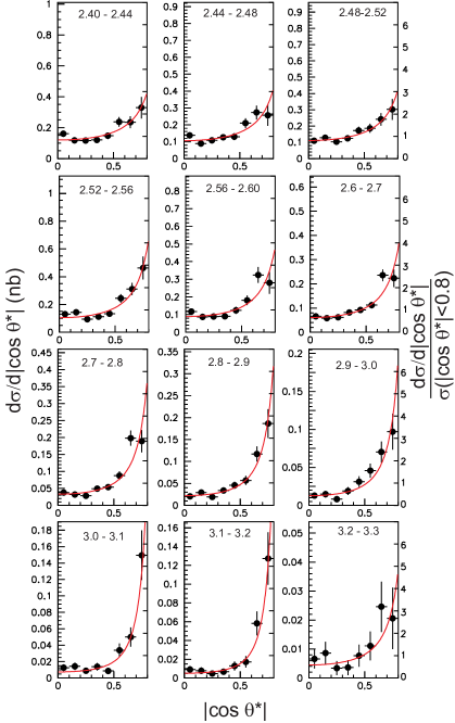
Figure 30: Data for the $\cos\theta^{*}$ dependence of the differential cross section and the results of the fits performed with the function proportional to $1/\sin^{\alpha}\theta^{*}$ (solid curve). The numbers in each panel show the $W$ region in GeV. The left (right) vertical scale of each subfigure corresponds to the absolute scale (normalized in such a way that the average is 1.25, as described in the text) of the differential cross section.

Figure 31: $W$ dependence of the parameter $\alpha$, which characterizes the angular dependence of the differential cross section. The horizontal line at $\alpha=4$ corresponds to the claim of the handbag model (see the text).

VIII.2 $W$ dependence

The $W$ dependence of the cross section integrated over the angle provides important information about the mechanism of the exclusive meson-pair production. We fit the cross section with

$$\sigma(|\cos\theta^{*}|<0.8)=aW^{-n}\;,$$ (22)

for the $W$ region 2.6 – 4.0 GeV, excluding 3.3 – 3.6 GeV. We exclude the region below 2.6 GeV because a resonance-like contribution is found there. We obtain $n=11.0\pm 0.4$. This result is shown by the dashed line in Fig. 32(a). The error is statistical only.

We also try the fits for the narrower $W$ region, 2.6 – 3.3 GeV, for $\sigma(|\cos\theta^{*}|<0.8)$ and $\sigma(|\cos\theta^{*}|<0.6)$, and obtain $n=10.0\pm 0.5$ and $n=11.8\pm 0.6$, respectively.

In our previous work, we obtained $n=10.5\pm 0.6$ for $W=2.4-4.0$ GeV excluding 3.3 – 3.6 GeV and $|\cos\theta^{*}|<0.6$ chen . The present analysis in this region yields $n=10.8\pm 0.2$. We quote this number only for verification, as we now know that it includes a resonance-like contribution around 2.5 GeV. These results are summarized in Table 17.

We estimate the systematic uncertainty for the $n$ measurement as follows: since the overall normalization error does not affect the determination of $n$, we consider the $W$-dependent distortion effect only. As in the resonance studies, we assume $\pm 4\%$ distortions at the two ends of the fit range and continuous variations between them. The distortion for a $W$ range changes the $n$ value with $\Delta n\approx\log 1.08/\log(W_{2}/W_{1})$, where $W_{1}$ and $W_{2}$ delimit the fit region (chosen to be 2.65 GeV and 3.25 GeV, respectively). We obtain the estimated systematic uncertainty $\Delta n=0.4$.

The slope parameter $n$ that ranges between 10 and 11 for the present process is larger than 6 and 7–8 that are predicted bl and observed nkzw , respectively, for the $\pi^{+}\pi^{-}$ and $K^{+}K^{-}$ processes. For the process $\gamma\gamma\to K^{0}_{S}K^{0}_{S}$, as discussed in Refs. chernyak ; chernyak2 , the coefficient of the leading-term amplitude is much smaller than that of the non-leading term. Therefore, at this energy the $W$ dependence of the cross section is mainly determined by that of the non-leading terms. In the $W$ region measured in this experiment and including a non-leading term, the perturbative QCD predicts $n=10$ chernyak2 , which is in reasonable agreement with our measurement.

Table 17: Results for the slope parameter $n$ from the power fit $\sigma\sim W^{-n}$ for $\gamma\gamma\to K^{0}_{S}K^{0}_{S}$ in different fit ranges. The result from the previous work chen is also shown. The first and second errors are statistical and systematic, respectively.

$W$ range (GeV)	$|\cos\theta^{*}|$ range	$n$	Note
$2.6-4.0$ (excluding $3.3-3.6$)	$<0.8$	$11.0\pm 0.4\pm 0.4$
$2.6-3.3$	$<0.8$	$10.0\pm 0.5\pm 0.4$
$2.6-3.3$	$<0.6$	$11.8\pm 0.6\pm 0.4$
$2.4-4.0$ (excluding $3.3-3.6$)	$<0.6$	$10.5\pm 0.6\pm 0.5$	Belle 2007

Figure 32: Results for the cross section integrated over $|\cos\theta^{*}|$ regions (a) below 0.8 and (b) below 0.6. The $W$ dependence is fitted to $W^{-n}$ in the different $W$ regions: 2.6 – 4.0 GeV excluding 3.3 – 3.6 GeV (dashed line) and 2.6 – 3.3 GeV (solid line).

IX Summary and conclusion

We have measured the cross section for the process $\gamma\gamma\rightarrow K^{0}_{S}K^{0}_{S}$ for $1.05~{}{\rm GeV}\leq W\leq 4.00~{}{\rm GeV}$ with the Belle detector at the asymmetric-energy KEKB collider. The data sample of 972 fb^-1 is three orders of magnitude larger than in the previous measurements tasso1 ; pluto ; cello ; tasso2 ; L3 . The differential cross section is measured up to $|\cos\theta^{*}|=0.8$, which allows high-sensitivity studies of the amplitudes.

In our study, the differential cross section has been fitted to obtain information on partial waves. The obtained spectra of $\hat{S}^{2}$, $\hat{D}_{0}^{2}$ and $\hat{D}_{2}^{2}$ indicate the presence of the $f_{0}(1710)$, $f_{J}(2200)$ and $f_{J^{\prime}}(2500)$ in addition to the well known $f_{2}(1270)$, $a_{2}(1320)$ and $f_{2}^{\prime}(1525)$. Then fits to the differential cross section are performed by assuming possible resonances in the partial waves.

First, we perform a fit in the region $1.15~{}{\rm GeV}\leq W\leq 1.65~{}{\rm GeV}$ to determine the parameters of the $f_{2}^{\prime}(1525)$ as well as the relative phase between the $f_{2}(1270)$ and $a_{2}(1320)$. Two solutions are obtained and combined statistically. The phase difference between the $a_{2}(1320)$ and $f_{2}(1270)$ is measured to be $\left(172.6^{+6.0+12.2}_{-0.7-7.0}\right)^{\circ}$, confirming the destructive interference between the two mesons and agreeing with theoretical predictions lipkin . The mass, total width and $\Gamma_{\gamma\gamma}{\cal B}(K\bar{K})$ of the $f_{2}^{\prime}(1525)$ are measured to be $1525.3^{+1.2+3.7}_{-1.4-2.1}$ MeV/$c^{2}$, $82.9^{+2.1+3.3}_{-2.2-2.0}$ MeV and $48^{+67+108}_{-8-12}$ eV, respectively. Note that no interference effect was taken into account in the previous measurements tasso1 ; pluto ; cello ; L3 .

Evidence for the existence of the $f_{0}(1710)$, $f_{2}(2200)$ and $f_{0}(2500)$ in this channel is obtained. Masses (widths) of these resonances are measured to be $1750^{+6+29}_{-7-18}$, $2243^{+7+3}_{-6-29}$, $2539\pm 14{}^{+38}_{-14}~{}{\rm MeV}/c^{2}$ ($139^{+11+96}_{-12-50}$, $145\pm 12{}^{+27}_{-34}$, $274^{+77+126}_{-61-163}~{}{\rm MeV}$), respectively. Their $\Gamma_{\gamma\gamma}{\cal B}(K\bar{K})$ values are measured for the first time to be $12^{+3+227}_{-2-8}$, $3.2^{+0.5+1.3}_{-0.4-2.2}$, $40^{+9+17}_{-7-40}~{}{\rm eV}$, respectively.

We conclude that the $f_{0}(1710)$ and $f_{2}(2200)$ are unlikely to be glueballs because their total widths and $\Gamma_{\gamma\gamma}{\cal B}(K\bar{K})$ values are much larger than those expected for a pure glueball state.

Analyses in the region $W>2.6~{}{\rm GeV}$ are updated; parameters of the $\chi_{c0}$ and $\chi_{c2}$ and the exponents $\alpha$ and $n$ in $(\sin\theta^{*})^{-\alpha}$ and $W^{-n}$ describing the angular and $W$ behavior of the cross section are extracted from data. The value of $\alpha$ does not show the tendency toward 4 observed in our previous work where the available angular region is limited to $|\cos\theta^{*}|<0.6$ chen . The fitted value of $n=11.0\pm 0.4\pm 0.4$ is much larger than the QCD asymptotic prediction of 6 or 7 bl but agrees fairly well with $n=10$ predicted by a qualitative QCD estimate chernyak2 . For the process $\gamma\gamma\to K^{0}_{S}K^{0}_{S}$, according to Refs. chernyak ; chernyak2 , the $W$ dependence of the cross section is determined by that of the non-leading term in the $W$ region measured by this experiment; the coefficient of the leading term amplitude is much smaller than that of the non-leading term. The results are consistent with the previous analyses chen with improved statistics and supersede the measurements for the cross section, the $\chi_{cJ}(1P)$ parameters and the slope parameter $n$.

We provide upper limits for the decay of the $\chi_{cJ}(2P)$, $\Gamma_{\gamma\gamma}(\chi_{c2}(2P)){\cal B}(\chi_{c2}(2P)\to K^{0}_{S}K^{0}_{S})<0.064$ eV and $\Gamma_{\gamma\gamma}(\chi_{c0}(2P)){\cal B}(\chi_{c0}(2P)\to K^{0}_{S}K^{0}_{S})<0.49$ eV at 90% CL, where the $\chi_{c0}(2P)$ coincides with the former $X(3915)$ pdg2012 ; pdg2013 . A new upper limit for the branching fraction of the $P$- and $CP$-violating decay $\eta_{c}\to K^{0}_{S}K^{0}_{S}$ is obtained to be $3.2\times 10^{-4}$ ($5.6\times 10^{-5}$) at 90% CL with (without) the interference effect.

References

(1)
T. Mori et al. (Belle Collaboration),
Phys. Rev. D 75, 051101(R) (2007).
(2) T. Mori et al. (Belle Collaboration),
J. Phys. Soc. Jpn 76, 074102 (2007).
(3)
H. Nakazawa et al. (Belle Collaboration),
Phys. Lett. B 615, 39 (2005).
(4)
K. Abe et al. (Belle Collaboration),
Eur. Phys. J. C 32, 323 (2004).
(5)
W.T. Chen et al. (Belle Collaboration),
Phys. Lett. B 651, 15 (2007).
(6)
C.C. Kuo et al. (Belle Collaboration),
Phys. Lett. B 621, 41 (2005).
(7)
S. Uehara et al. (Belle Collaboration),
Phys. Rev. Lett. 96, 082003 (2006).
(8)
S. Uehara, Y. Watanabe et al. (Belle Collaboration),
Phys. Rev. D 78, 052004 (2008).
(9) S. Uehara, Y. Watanabe,
H. Nakazawa et al. (Belle Collaboration),
Phys. Rev. D 79, 052009 (2009).
(10) S. Uehara, Y. Watanabe,
H. Nakazawa et al. (Belle Collaboration),
Phys. Rev. D 80, 032001 (2009).
(11) S. Uehara, Y. Watanabe,
H. Nakazawa et al. (Belle Collaboration),
Phys. Rev. D 82, 073011 (2010).
(12) See, e.g., the compilation in
http://durpdg.dur.ac.uk/review/2gamma/.