Dynamical evolution of the electromagnetic perturbation with Weyl corrections

Abstract

Abstract

We present firstly the master equation of an electromagnetic perturbation with Weyl correction in the four-dimensional black hole spacetime, which depends not only on the Weyl correction parameter, but also on the parity of the electromagnetic field. It is quite different from that of the usual electromagnetic perturbation without Weyl correction in the four-dimensional spacetime. And then we have investigated numerically the dynamical evolution of the electromagnetic perturbation with Weyl correction in the background of a four-dimensional Schwarzschild black hole spacetime. Our results show that the Weyl correction parameter $\alpha$ and the parities imprint in the wave dynamics of the electromagnetic perturbation. For the odd parity electromagnetic perturbation, we find it grows with exponential rate if the value of $\alpha$ is below the negative critical value $\alpha_{c}$. However, for the electromagnetic perturbation with even parity, we find that there does not exist such a critical threshold value and the electromagnetic field always decays in the allowed range of $\alpha$.

I Introduction

For the last few decades, one of most interesting topics is to study the dynamical evolution of an external perturbation around a black hole. It is widely believed that the quasinormal modes in the dynamical evolution carry the characteristic information about the black hole and could help us to identify whether there exists black hole in our Universe or not Chandrasekhar:1975 ; Nollert:1999 ; Kokkotas:1999 . The further investigations imply that the quasinormal spectrum of black holes could open a window for us to understand more deeply about the quantum gravity Hod:1998 ; Dreyer:2003 ; Corichi:2003 and the AdS/CFT correspondence Maldacena:1998 ; Witten:1998 ; Horowitz:2000 . Moreover, the dynamical behaviors of the perturbations could be used to test the stability of a black hole in various theories of gravity Gregory:1993 ; Harmark:2007 ; Konoplya:2008 ; Chen:2009 . The dynamical evolution of various perturbations have been studied extensively in the various black holes spacetime Price:1972 ; Hod:1998ja ; Burko2003 ; Koyama:2001 ; Hod:1998ma ; Cardoso2001 ; Barack:2000 .

All of the above investigations mentioned for the electromagnetic perturbation are in the frame of Einstein-Maxwell electromagnetic theory in which the Maxwell Lagrangian is only quadratic in the Maxwell tensor and does not contain any coupling between the Maxwell part and the curvature part. Recently, a lot of attention have been focused on studying the generalized Einstein-Maxwell theory. The main motivation is that the generalized Einstein-Maxwell theory contains higher derivative interactions and carries more information about the electromagnetic field. The study of the generalized Einstein-Maxwell theory could help us to explore the full properties and effects of the electromagnetic fields. One of interesting generalized Einstein-Maxwell theory is Born-Infeld theory which is introduced in the thirties Born in order to remove the divergence of the electron’s self-energy in the classical electrodynamics. Moreover, Born-Infeld theory displays good physical properties concerning wave propagation such as the absence of shock waves and birefringence phenomena Boillat . Born-Infeld theory has also received special attention because it could arise in the low-energy regime of string and D-Brane physics Fradkin . Another generalization of the Einstein-Maxwell theory with three parameters has been considered in which there are the non-minimal couplings between the gravitational and electromagnetic fields in the Lagrangian Balakin ; Faraoni ; Hehl ; Balakin1 . The presence of such non-minimal couplings in the Lagrangian modifies of the coefficients involving the second-order derivatives both in the Maxwell and Einstein equations, which could affect the propagation of gravitational and electromagnetic waves in the spacetime and may yield time delays in the arrival of those waves Balakin . Moreover, these couplings could modify the electromagnetic and gravitational structure of a charged black hole Balakin1 . In the evolution of the early Universe, these coupled terms may yield electromagnetic quantum fluctuations and lead to the inflation Turner ; Mazzitelli ; Lambiase ; Raya ; Campanelli . Due to the inflation at that time, the scale of the fluctuations can be stretched towards outside the Hubble horizon and then they result in classical fluctuations, which means that the non-minimal couplings could be used to explain the large scale magnetic fields observed in clusters of galaxies Bamba ; Kim ; Clarke .

In this paper, we consider a simple generalized electromagnetic theory which involves a coupling between the Maxwell field and the Weyl tensor Weyl1 ; Drummond . In this theory, the Lagrangian density of the electromagnetic field is modified as

$$L_{EM}=-\frac{1}{4}\bigg{(}F_{\mu\nu}F^{\mu\nu}-4\alpha C^{\mu\nu\rho\sigma}F_{\mu\nu}F_{\rho\sigma}\bigg{)},$$ (1)

where $C_{\mu\nu\rho\sigma}$ is the Weyl tensor and $\alpha$ is a coupling constant with dimensions of length-squared. $F_{\mu\nu}$ is the electromagnetic tensor, which is related to the electromagnetic vector potential $A_{\mu}$ by $F_{\mu\nu}=A_{\nu;\mu}-A_{\mu;\nu}$. Actually, the coupling in the Lagrangian density (1) is a special of coupling between the gravitational and electromagnetic fields since Weyl tensor $C_{\mu\nu\rho\sigma}$ is related to the Riemann tensor $R_{\mu\nu\rho\sigma}$, the Ricci tensor $R_{\mu\nu}$ and the Ricci scalar $R$ by

$$C_{\mu\nu\rho\sigma}=R_{\mu\nu\rho\sigma}-\frac{2}{n-2}(g_{\mu[\rho}R_{\sigma]\nu}-g_{\nu[\rho}R_{\sigma]\mu})+\frac{2}{(n-1)(n-2)}Rg_{\mu[\rho}g_{\sigma]\nu},$$ (2)

where $n$ and $g_{\mu\nu}$ are the dimension and metric of the spacetime, and brackets around indices refers to the antisymmetric part. It was found that the similar couplings between curvature tensor and Maxwell tensor could be obtained from a calculation in QED of the photon effective action from one-loop vacuum polarization on a curved background Drummond . Although Weyl correction can be looked as an effective description of quantum effects, such kind of couplings may also occur near classical compact astrophysical objects with high mass density and strong gravitational field such as the supermassive black holes at the center of galaxies Dereli1 . The effects originating from such kind of couplings could also be used to distinguish between general relativity and other theories of gravity in the future astrophysical observations Solanki . Therefore, we can treat the Weyl correction to electromagnetic field as a kind of general classical couplings between the gravitational and electromagnetic fields and study the effects of such correction on the dynamical evolution of electromagnetic field in the general background spacetime. The coupling term with Weyl tensor is a tensorial structure correcting the Maxwell term at leading order in derivatives, which modifies the Einstein-Maxwell equation and affects the dynamical evolution of electromagnetic field in the background spacetime. An advantage of this generalized electromagnetic theory with Weyl correction is that the modified Einstein-Maxwell equation is not complicated and the equations of motion for electromagnetic perturbation can be decoupled to a second order differential equation, which is very important for us to investigate further the dynamical properties of electromagnetic perturbation in the black hole spacetime. In Ref.Weyl1 , the authors studied the holographic conductivity and charge diffusion with Weyl correction in the anti-de Sitter (AdS) spacetime and found that the correction breaks the universal relation with the $U(1)$ central charge observed at leading order. Recently, the holographic superconductors with Weyl corrections are also explored in Wu2011 ; Ma2011 ; Momeni ; Roychowdhury . Wu et al Wu2011 studied the effects of Weyl corrections $s$-wave holographic superconductor and found that with Weyl corrections the critical temperature becomes smaller and the scalar hair is formed harder when the coupling constant $\alpha$ is negative, but the result is just opposite when the constant $\alpha$ is positive. In the Stückelberg mechanism, it is found that Weyl coupling parameter $\alpha$ also changes the order of the phase transition of the holographic superconductor Ma2011 . The $p$-wave holographic superconductor model with Weyl corrections has been studied and it is shown that the effect of Weyl corrections on the condensation is similar to that of the $s$-wave model Momeni . Moreover, the effects of Weyl corrections on the phase transition between the holographic insulator and superconductor has been investigated in zhao2013 and it is found that in this case the effects of Weyl corrections depend on the model of holographic dual. For the $p$-wave model, the higher Weyl corrections will make it harder for the holographic insulator/superconductor phase transition to be triggered. However, for the $s$-wave model, the Weyl couplings do not affect the properties of the holographic insulator/superconductor phase transition since the critical chemical potentials are independent of the Weyl correction terms in this case. These results may excite more efforts to be focused on the study of the electrodynamics with Weyl corrections in the more general cases. The main purpose of this paper is to investigate the dynamical evolution of the electromagnetic perturbation coupling to the Weyl tensor in the Schwarzschild black hole spacetime and see the effect of the Weyl corrections on the stability of the black hole.

The plan of our paper is organized as follows: in the following section we will derive the master equation of electromagnetic perturbation with Weyl correction in the four-dimensional static and spherical symmetric spacetime. In Sec.III, we will study numerically the effects of the Weyl corrections on the quasinormal modes of the electromagnetic perturbation in the Schwarzschild black hole and then examine the stability of the black hole. Finally, in the last section we will include our conclusions.

II The wave equation for the electromagnetic perturbations with Weyl corrections

In order to study the effects of Weyl corrections on the dynamical evolution of the electromagnetic perturbations in a black hole spacetime, we must first obtain its wave equation in the background. The action of Maxwell field with Weyl corrections in the curved spacetime has a form Weyl1

$$S=\int d^{4}x\sqrt{-g}\bigg{[}\frac{R}{16\pi G}-\frac{1}{4}\bigg{(}F_{\mu\nu}F^{\mu\nu}-4\alpha C^{\mu\nu\rho\sigma}F_{\mu\nu}F_{\rho\sigma}\bigg{)}\bigg{]}.$$ (3)

Varying the action (3) with respect to $A_{\mu}$, one can obtain the generalized Maxwell equation

$$\nabla_{\mu}\bigg{(}F^{\mu\nu}-4\alpha C^{\mu\nu\rho\sigma}F_{\rho\sigma}\bigg{)}=0.$$ (4)

Obviously, the Weyl corrections affect the dynamical evolution of the electromagnetic perturbation.

For a four-dimensional static and spherical symmetric black hole spacetime, the metric has a form

$$ds^{2} = fdt^{2}-\frac{1}{f}dr^{2}-r^{2}d\theta^{2}-r^{2}\sin^{2}{\theta}d\phi^{2},$$ (5)

where the metric coefficient $f$ is a function of polar coordinate $r$. In this background, one can expand $A_{\mu}$ in vector spherical harmonics Ruffini

$$A_{\mu}=\sum_{l,m}\left(\left[\begin{array}[]{ccc}&0&\\ &0&\\ &\frac{a^{lm}(t,r)}{\sin\theta}\partial_{\phi}Y_{lm}&\\ &-a^{lm}(t,r)\sin\theta\partial_{\theta}Y_{lm}&\end{array}\right]+\left[\begin{array}[]{cccc}&j^{lm}(t,r)Y_{lm}&\\ &h^{lm}(t,r)Y_{lm}&\\ &k^{lm}(t,r)\partial_{\theta}Y_{lm}&\\ &k^{lm}(t,r)\partial_{\phi}Y_{lm}&\end{array}\right]\right),$$ (14)

where the first term in the right side has parity $(-1)^{l+1}$ and the second term has parity $(-1)^{l}$, $l$ is the angular quantum number and $m$ is the azimuthal number.

Adopting the following form

$$a^{lm}(t,r) = a^{lm}(r)e^{-i\omega t},~{}~{}~{}~{}~{}h^{lm}(t,r)=h^{lm}(r)e^{-i\omega t},$$

$$j^{lm}(t,r) = j^{lm}(r)e^{-i\omega t},~{}~{}~{}~{}~{}k^{lm}(t,r)=k^{lm}(r)e^{-i\omega t},$$ (15)

and then inserting the above expansion (14) into the generalized Maxwell equation (4), we can obtain three independent coupled differential equations. Eliminating $k^{lm}(r)$, we can get a second order differential equation for the perturbation

$$\frac{d^{2}\Psi(r)}{dr^{2}_{*}}+[\omega^{2}-V(r)]\Psi(r)=0,$$ (16)

where the tortoise coordinate $r_{*}$ is defined as $dr_{*}=\frac{dr}{f}$. The wavefunction $\Psi(r)$ is a linear combination of the functions $j^{lm}$, $h^{lm}$, and $a^{lm}$, which appeared in the expansion (14). The form of $\Psi(r)$ depends on the parity of the perturbation, which can be expressed as

$$\Psi(r)=a^{lm}\sqrt{1+\frac{2\alpha}{3r^{2}}(r^{2}f^{\prime\prime}-2rf^{\prime}+2f-2)},$$ (17)

for the odd parity $(-1)^{l+1}$, and

$$\Psi(r)=\frac{r^{2}}{l(l+1)}\bigg{(}-i\omega h^{lm}-\frac{dj^{lm}}{dr}\bigg{)}\frac{\sqrt{1-\frac{2\alpha}{3r^{2}}(r^{2}f^{\prime\prime}-2rf^{\prime}+2f-2)}}{1-\frac{4\alpha}{3r^{2}}(r^{2}f^{\prime\prime}-2rf^{\prime}+2f-2)},$$ (18)

for the even parity $(-1)^{l}$, respectively. The effective potential $V(r)$ in Eq. (16) depends also on the parity of the perturbation. For the odd parity, the potential $V(r)$ is given by

$$V(r)=f\bigg{\{}\frac{l(l+1)}{r^{2}}\frac{1-\frac{4\alpha}{3r^{2}}(r^{2}f^{\prime\prime}-2rf^{\prime}+2f-2)}{1+\frac{2\alpha}{3r^{2}}(r^{2}f^{\prime\prime}-2rf^{\prime}+2f-2)}+\frac{\alpha(h_{0}+h_{1}\alpha)}{r^{2}[3r^{2}+2\alpha(r^{2}f^{\prime\prime}-2rf^{\prime}+2f-2)]^{2}}\bigg{\}},$$ (19)

whereas for the even parity it is given by

$$V(r)=f\bigg{\{}\frac{l(l+1)}{r^{2}}\frac{1+\frac{2\alpha}{3r^{2}}(r^{2}f^{\prime\prime}-2rf^{\prime}+2f-2)}{1-\frac{4\alpha}{3r^{2}}(r^{2}f^{\prime\prime}-2rf^{\prime}+2f-2)}-\frac{\alpha(h_{0}+h_{2}\alpha)}{r^{2}[3r^{2}+2\alpha(r^{2}f^{\prime\prime}-2rf^{\prime}+2f-2)]^{2}}\bigg{\}},$$ (20)

where

$$h_{0} = 3r^{2}[12f^{2}+rf^{\prime}(r^{3}f^{(3)}-2r^{2}f^{\prime\prime}+4rf^{\prime}+4)+f(r^{4}f^{(4)}-2r^{3}f^{(3)}+6r^{2}f^{\prime\prime}-16rf^{\prime}-12)],$$ (21)

$$h_{1} = 32f^{3}+2rf^{\prime}(r^{2}f^{\prime\prime}-2rf^{\prime}-2)(r^{3}f^{(3)}-2r^{2}f^{\prime\prime}+4rf^{\prime}+4)+4f^{2}(r^{4}f^{(4)}+8r^{2}f^{\prime\prime}-20rf^{\prime}-16)$$ (22)

$$- f[4r^{4}f^{(4)}+(r^{3}f^{(3)})^{2}-8r^{4}f^{\prime\prime 2}-64r^{2}f^{\prime 2}-32+4rf^{\prime}(r^{4}f^{(4)}-r^{3}f^{(3)}+12r^{4}f^{\prime\prime}-24)$$

$$+ 2r^{2}f^{\prime\prime}(16-r^{4}f^{(4)})],$$

$$h_{2} = -16r^{3}f^{\prime 3}-4r^{2}f^{\prime 2}(r^{3}f^{(3)}-4r^{2}f^{\prime\prime}-8rf^{\prime}+8)+r^{2}f[2(4f^{(3)}+rf^{(4)})(r^{2}f^{\prime\prime}+2f-2)-3r^{3}(f^{(3)})^{2}]$$ (23)

$$- 2f^{\prime}[8f^{2}-(r^{2}f^{\prime\prime}-2)(r^{3}f^{(3)}-2r^{2}f^{\prime\prime}+4)+2f(r^{4}f^{(4)}+3r^{3}f^{(3)}+4r^{2}f^{\prime\prime}-8)].$$

It is clear that the coupling constant $\alpha$ emerges in the effective potential, which means that Wely corrections will change the dynamical evolution of the electromagnetic perturbation in the background spacetime. From Eqs. (19) and (20), we also find that the modification of the effective potential by Weyl corrections is different for the electromagnetic perturbations with different parities, which implies that the effects of Weyl corrections on the wave dynamics for the electromagnetic perturbation with the odd parity are different from those of the perturbation with the even parity. This is quite different from that in the case of the usual electromagnetic perturbation without Weyl corrections in the four-dimensional spacetime, in which the electromagnetic perturbation with the odd parity has the same effective potential as for the perturbation with the even parity. When the coupling constant $\alpha=0$ the effective potentials (19) and (20) recover to the usual form without Weyl corrections.

III Effects of Weyl corrections on the wave dynamics of the electromagnetic perturbation in the Schwarzschild black hole spacetime

In this section, we will study numerically the dynamical evolution of the electromagnetic perturbation with Weyl corrections in the background of a Schwarzschild black hole spacetime and probe the effects of Weyl corrections on the wave dynamics of the electromagnetic perturbation.

For the Schwarzschild black hole spacetime, the metric function is $f=1-\frac{2M}{r}$ and then the effective potentials (19) and (20) can be expressed as

$$V(r)_{odd}=(1-\frac{2M}{r})\bigg{[}\frac{l(l+1)}{r^{2}}(\frac{r^{3}+16\alpha M}{r^{3}-8\alpha M})-\frac{24\alpha M(2r^{4}-5Mr^{3}-10\alpha Mr+28\alpha M^{2})}{r^{3}(r^{3}-8\alpha M)^{2}}\bigg{]},$$ (24)

for the odd parity and

$$V(r)_{even}=(1-\frac{2M}{r})\bigg{[}\frac{l(l+1)}{r^{2}}(\frac{r^{3}-8\alpha M}{r^{3}+16\alpha M})+\frac{24\alpha M(2r^{4}-5Mr^{3}+2\alpha Mr+4\alpha M^{2})}{r^{3}(r^{3}-8\alpha M)^{2}}\bigg{]},$$ (25)

for the even parity, respectively. Defining the quantity

$$W = \frac{12\alpha M(r-2M)}{r^{2}(r^{3}-8\alpha M)}+\frac{3l(l+1)}{4r}+\frac{\sqrt{3}l(l+1)}{16\alpha^{3}M^{3}}\bigg{[}4\arctan\bigg{(}\frac{r+(\alpha M)^{\frac{1}{3}}}{\sqrt{3}(\alpha M)^{\frac{1}{3}}}\bigg{)}-2^{\frac{2}{3}}\arctan\bigg{(}\frac{2^{\frac{1}{3}}r-2(\alpha M)^{\frac{1}{3}}}{2\sqrt{3}(\alpha M)^{\frac{1}{3}}}\bigg{)}\bigg{]}$$ (26)

$$+ \frac{l(l+1)}{32\alpha^{3}M^{3}}\bigg{\{}4\log\bigg{[}\frac{(r-2(\alpha M)^{\frac{1}{3}})^{2}}{r^{2}+2(\alpha M)^{\frac{1}{3}}r+4(\alpha M)^{\frac{2}{3}}}\bigg{]}+2^{\frac{2}{3}}\log\bigg{[}\frac{(2^{\frac{2}{3}}r+4(\alpha M)^{\frac{1}{3}})^{2}}{2^{\frac{1}{3}}r^{2}-2^{\frac{5}{3}}(\alpha M)^{\frac{1}{3}}r+8(\alpha M)^{\frac{2}{3}}}\bigg{]}\bigg{\}},$$

we can obtain

$$V(r)_{odd}=W^{2}+\frac{dW}{dr_{*}}+\beta,~{}~{}~{}~{}~{}~{}~{}~{}~{}~{}V(r)_{even}=W^{2}-\frac{dW}{dr_{*}}+\beta,$$ (27)

with

$$\beta=\frac{(r-2M)}{r^{3}(r^{3}-8\alpha M)}\bigg{[}\frac{r^{6}+8\alpha M+160\alpha^{2}M^{2}}{(r^{3}+16\alpha M)}+\frac{144\alpha^{2}M^{2}(r-2M)}{r(r^{3}-8\alpha M)}\bigg{]}-W^{2}.$$ (28)

This means that these two effective potentials for odd and even parities can be written in the form of super-partner potentials. The similar behavior of effective potentials for gravitational perturbations have been discovered in Chandrasekhar1983 ; Cooper1995 .

Figure 1: Variation of the effective potential $V(r)_{odd}$ with the polar coordinate $r$ for fixed $l=1$ (left), $l=2$ (middle) and $l=3$ (right). The long-dash-dotted, dashed, solid, dotted and short-dash-dotted lines are corresponding to the cases with $\alpha=-0.4,\;-0.2,\;0,\;0.1\;0.2$, respectively. We set $2M=1$.

Figure 2: Variation of the effective potential $V(r)_{even}$ with the polar coordinate $r$ for fixed $l=1$ (left), $l=2$ (middle) and $l=3$ (right). The long-dash-dotted, dashed, solid, dotted and short-dash-dotted lines are corresponding to the cases with $\alpha=-0.1,\;-0.05,\;0,\;0.1\;0.2$, respectively. We set $2M=1$.

Considering that the effective potential should be continuous in the region outside the event horizon of black hole, the coupling constant $\alpha$ must satisfy $r^{3}_{H}-8\alpha M>0$ (i.e., $\alpha<M^{2}$) for the electromagnetic perturbation with the odd parity, and satisfy $r^{3}_{H}-8\alpha M>0$ and $r^{3}_{H}+16\alpha M>0$ (i.e., $-\frac{M^{2}}{2}<\alpha<M^{2}$) for the perturbation with the even parity. In Figs.(1) and (2), we show the changes of the effective potentials $V(r)_{odd}$ and $V(r)_{even}$ with the coupling constant $\alpha$ for fixed $l$, respectively. For fixed $l$, the peak height of the potential barrier increases with the coupling constant $\alpha$ for $V(r)_{odd}$ and decreases for $V(r)_{even}$. Moreover, we also find that there exits the negative gap in the effective potential $V(r)_{odd}$ only for the certain negative value of $\alpha$ and in the potential $V(r)_{even}$ only for the certain positive value of $\alpha$. This means that the properties of the wave dynamics of the electromagnetic perturbation with the odd parity could be different from those of that with the even parity. In the following section, we will check those values of $\alpha$ for which the negative gap is present and study the stability of the black hole under the electromagnetic perturbation with Weyl corrections.

Let us now to study the effects of the Weyl corrections on the quasinormal modes of electromagnetic perturbation in the Schwarzschild black hole spacetime. In Fig. (3) and (4), we present the fundamental quasinormal modes ($n=0$) evaluated by the third-order WKB approximation method Schutz:1985 ; Iyer:1987 . It is shown that with the increase of the coupling parameter $\alpha$ the real parts of the quasinormal frequencies increase for the electromagnetic perturbation with the odd parity, but decrease for that with the even parity. The changes of the imaginary parts with $\alpha$ are more complicated. For the odd parity electromagnetic perturbation, we find that as $\alpha<0$ the imaginary part of increases with $\alpha$. When $\alpha>0$, the imaginary part for $l=1$ first decreases to the minimum and then rises to the maximum and subsequently decreases to another minimum, and finally it increases again with $\alpha$, while for other $l$ it first decreases and then increases. For the even parity electromagnetic perturbation, we find that with the increase of $\alpha$ the imaginary part of first decreases and then increases as $\alpha>0$. When $\alpha<0$, with the increase of $\alpha$ the imaginary part for $l=1$ first decreases to the minimum and then rises to the maximum and subsequently decreases to another minimum, and finally it increases again to another maximum, while for other $l$ it first decreases and then increases. These results imply that Weyl corrections modify the standard results of the quasinormal modes for the electromagnetic perturbations in the background of a Schwarzschild black hole.

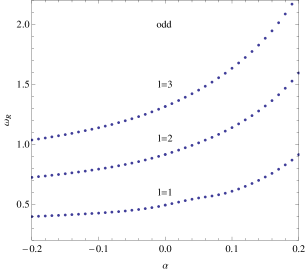
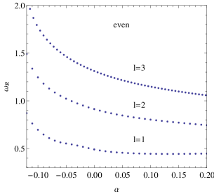
Figure 3: Effects of Weyl corrections on the real parts of the fundamental quasinormal modes of electromagnetic perturbation with the odd parity(the left) or the even parity (the right) in the Schwarzschild black hole spacetime. We set $2M=1$.

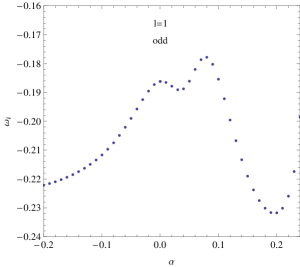
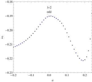
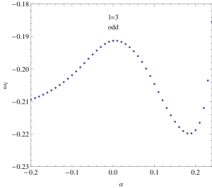
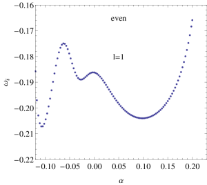
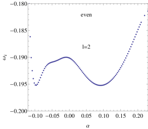
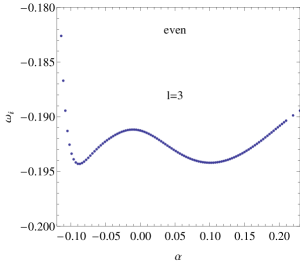
Figure 4: Effects of Weyl corrections on the imaginary parts of the fundamental quasinormal modes of electromagnetic perturbation with the odd parity(the top row) or the even parity (the bottom row) in the Schwarzschild black hole spacetime. We set $2M=1$.

Now we are in a position to study the dynamical evolution of the electromagnetic perturbation with Weyl corrections in time domain Gundlach:1994 and examine the stability of the Schwarzschild black hole in this cases. Making use of the light-cone variables $u=t-r_{*}$ and $v=t+r_{*}$, one can find that the wave equation

$$-\frac{\partial^{2}\psi}{\partial t^{2}}+\frac{\partial^{2}\psi}{\partial r_{*}^{2}}=V(r)\psi,$$ (29)

can be rewritten as

$$4\frac{\partial^{2}\psi}{\partial u\partial v}+V(r)\psi=0.$$ (30)

It is well known that the two-dimensional wave equation (30) can be integrated numerically by using the finite difference method suggested in Gundlach:1994 . From Taylor’s theorem, we can find that the wave equation (30) can be discretized as

$$\psi_{N}=\psi_{E}+\psi_{W}-\psi_{S}-\delta u\delta vV(\frac{v_{N}+v_{W}-u_{N}-u_{E}}{4})\frac{\psi_{W}+\psi_{E}}{8}+O(\epsilon^{4})=0.$$ (31)

Here we have used the following definitions for the points: $N$: $(u+\delta u,v+\delta v)$, $W$: $(u+\delta u,v)$, $E$: $(u,v+\delta v)$ and $S$: $(u,v)$. The parameter $\epsilon$ is an overall grid scalar factor, so that $\delta u\sim\delta v\sim\epsilon$. As in Gundlach:1994 , we can set $\psi(u,v=v_{0})=0$ and use a Gaussian pulse as an initial perturbation, centered on $v_{c}$ and with width $\sigma$ on $u=u_{0}$ as

$$\psi(u=u_{0},v)=e^{-\frac{(v-v_{c})^{2}}{2\sigma^{2}}}.$$ (32)

Figure 5: The dynamical evolution of an electromagnetic perturbation with odd parity in the background of a Schwarzschild black hole spacetime. The figures from left to right are corresponding to $l=1$, $2$ and $3$. The dotted, solid, dash-dotted and dashed lines are corresponding to the cases with $\alpha=0.2,~{}0,~{}-0.2,~{}-0.3$, respectively. We set $2M=1$.The constants in the Gauss pulse (32) $v_{c}=10$ and $\sigma=3$.

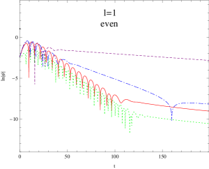
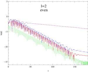
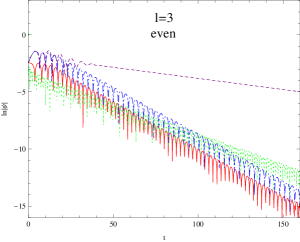
Figure 6: The dynamical evolution of an electromagnetic perturbation with even parity in the background of a Schwarzschild black hole spacetime. The figures from left to right are corresponding to $l=1$, $2$ and $3$. The dotted, solid, dash-dotted and dashed lines are corresponding to the cases with $\alpha=-0.12,~{}0,~{}0.20,~{}0.24$, respectively. We set $2M=1$.The constants in the Gauss pulse (32) $v_{c}=10$ and $\sigma=3$.

In figs. (5) and (6), we present the dynamical evolution of an electromagnetic perturbation with Weyl correction in the background of a Schwarzschild black hole. Our result show that the effects of Weyl correction on the dynamical evolution of the odd parity electromagnetic perturbation are different from those of the even parity electromagnetic one. For the electromagnetic perturbation with odd parity, one can that as $\alpha>0$ the decay of the electromagnetic perturbation with the Weyl correction is similar to that of the electromagnetic one without Weyl correction, which indicates that the black hole is stable. It is understandable by a fact that the effective potential $V(r)$ is positive definite, which is shown in fig.(1). When $\alpha<0$, we find that the electromagnetic field grows with exponential rate if the coupling constant $\alpha$ is smaller than the critical value $\alpha_{c}$. It means that the instability occurs in this case. The main reason is that for the odd parity electromagnetic perturbation with negative coupling constant $\alpha$ the large absolute value of $\alpha$ drops down the peak of the potential barrier and increases the negative gap near the black hole horizon so that the potential could be non-positive definite. In the instability region, we can find that for the larger $|\alpha|$ the instability growth appears more early and the growth rate becomes stronger. For the electromagnetic perturbation with even parity, we find that the electromagnetic field always decays in the allowed range of $\alpha$. Although in the effective potential $V(r)_{even}$ the negative gap appears near the black hole horizon as $\alpha>0$ and increases with $\alpha$, the negative gap is very small in this case, which is not enough to yield the instability to be triggered.

In fig.(7), we plotted the change of the threshold value $\alpha_{c}$ with $l$ for the odd parity electromagnetic perturbation with Weyl corrections, and found that the threshold value can be fitted best by the function

$$\alpha_{c}\simeq a\sqrt{\frac{l}{l+1}}+b,$$ (33)

where the coefficients $a$ and $b$ are numerical constants with dimensions of length-squared and their values are $a=0.5534$ and $b=-0.6785$.

Figure 7: The change of the threshold value $\alpha_{c}$ with the multipole number $l$. The points $l=1\sim 20$ are fitted by the function $\alpha_{c}=a~{}\sqrt{\frac{l}{l+1}}+b$, where the coefficients $a$ and $b$ are numerical constants with dimensions of length-squared and their values are $a=0.5534$ and $b=-0.6785$.

It is easy to obtain that the threshold value $\alpha_{c}$ is negative and increases with the multipole number $l$. This means that for the higher $l$ we need the smaller Weyl corrections at which instability happens. From Eq. (33), we can obtain that in the limit $l\rightarrow\infty$ the threshold value $\alpha_{c}\rightarrow a+b=-0.1251$. It could be explained by a fact that in this limit the effective potential (24) has the form

$$V(r)|_{l\rightarrow\infty}=f\frac{l(l+1)}{r^{2}}\bigg{(}\frac{r^{3}+16\alpha M}{r^{3}-8\alpha M}\bigg{)},$$ (34)

which leads to the integration Gleiser:2005 ,

$$\int^{\infty}_{r_{+}}\frac{V(r)|_{l\rightarrow\infty}}{f}dr=\int^{\infty}_{r_{+}}\bigg{(}\frac{r^{3}+16\alpha M}{r^{3}-8\alpha M}\bigg{)}\frac{l(l+1)}{r^{2}}dr,$$ (35)

is positive definite as $\alpha<-r^{3}_{+}/(16M)$. It implies that the threshold value has a form $\alpha_{c}=-M^{2}/2$ as $l\rightarrow\infty$, which is consistent with the form of the numerical constant $a+b$ obtained in the previous numerical calculation.

IV summary

In this paper, we present firstly the master equation of an electromagnetic perturbation with Weyl correction in the four-dimensional black hole spacetime and find that the presence of Weyl corrections makes that the master equation of the odd parity electromagnetic perturbation is different from that of the even parity one, which is quite different from that of the usual electromagnetic perturbation without Weyl correction in the four-dimensional spacetime where the master equation is independent of the parity of the electromagnetic field. And then we have investigated numerically the dynamical evolution of an electromagnetic perturbation with Weyl correction in the background of a four-dimensional Schwarzschild black hole spacetime. Our results show that the Weyl correction modifies the standard results of the wave dynamics for the electromagnetic perturbation. Due to the presence of Weyl corrections, the dynamical properties of the electromagnetic perturbation depend not only on the Weyl correction parameter $\alpha$, but also on the parity of the electromagnetic field. With the increase of $\alpha$, the real part of the fundamental quasinormal frequencies for fixed $l$ increases for the odd parity electromagnetic perturbation and decreases for the event parity electromagnetic one. The changes of the imaginary parts with $\alpha$ are more complicated. Moreover, we find that the odd parity electromagnetic perturbation grows with exponential rate if the coupling constant $\alpha$ is smaller than the negative critical value $\alpha_{c}$. This means that the instability occurs in this case. In the instability region, we can find that for the smaller $\alpha$ the instability growth appears more early and the growth rate becomes stronger. For the electromagnetic perturbation with even parity, we find that the electromagnetic field always decays in the allowed range of $\alpha$. Although in the effective potential $V(r)_{even}$ the negative gap appears near the black hole horizon as $\alpha>0$, the negative gap is very small and is not enough to yield the occurrence of instability in this case.

Furthermore, we find that the threshold value can be fitted best by the function $\alpha_{c}\simeq a\sqrt{\frac{l}{l+1}}+b$ with two numerical constants (with dimensions of length-squared) $a,b$. These rich dynamical properties of the electromagnetic perturbation with Weyl correction, at least in principle, may provide a possibility to detect whether there exists Weyl correction to electromagnetic field or not in the future astronomical observations, such as the future space-based detector LISA etc. It would be of interest to generalize our study to other black hole spacetimes, such as rotating black holes etc. Work in this direction will be reported in the future.

V Acknowledgments

This work was partially supported by the National Natural Science Foundation of China under Grant No.11275065, the NCET under Grant No.10-0165, the PCSIRT under Grant No. IRT0964, the Hunan Provincial Natural Science Foundation of China (11JJ7001) and the construct program of key disciplines in Hunan Province. J. Jing’s work was partially supported by the National Natural Science Foundation of China under Grant Nos. 11175065, 10935013; 973 Program Grant No. 2010CB833004.

References

- (1) S. Chandrasekhar and S. Detweller, Proc. R. Soc. Lond. A 344, 441 (1975).
- (2) H. P. Nollert, Class. Quantum Grav. 16, R159 (1999).
- (3) K. D. Kokkotas and B. G. Schmidt, Living Rev. Rel. 2, 2 (1999).
- (4) S. Hod, Phys. Rev. Lett. 81, 4293 (1998).
- (5) O. Dreyer, Phys. Rev. Lett. 90, 081301 (2003).
- (6) A. Corichi, Phys. Rev. D 67, 087502 (2003); L. Motl, Adv. Theor. Math. Phys. 6, 1135 (2003); L. Motl and A. Neitzke, Adv. Theor. Math. Phys. 7, 307 (2003); A. Maassen van den Brink, J. Math. Phys. 45, 327 (2004); G. Kunstatter, Phys. Rev. Lett. 90, 161301 (2003); N. Andersson and C. J. Howls, Class. Quantum Grav. 21, 1623 (2004); V. Cardoso, J. Natario and R. Schiappa, J. Math. Phys. 45, 4698 (2004); J. Natario and R. Schiappa, Adv. Theor. Math. Phys. 8, 1001 (2004); V. Cardoso and J. P. S. Lemos, Phys. Rev. D 67, 084020 (2003).
- (7) J. Maldacena, Adv. Theor. Math. Phys. 2, 231 (1998).
- (8) E. Witten, Adv. Theor. Math. Phys. 2, 253 (1998).
- (9) G. T. Horowitz and V. E. Hubeny, Phys. Rev. D 62, 024027 (2000); B. Wang, C. Y. Lin and E. Abdalla, Phys. Lett. B 481, 79 (2000) ; J. M. Zhu, B. Wang and E. Abdalla, Phys. Rev. D 63, 124004 (2001); V. Cardoso and J. P. S. Lemos, Phys. Rev. D 63, 124015 (2001); V. Cardoso and J. P. S. Lemos, Phys. Rev. D 64, 084017 (2001); E. Berti and K. D. Kokkotas, Phys. Rev. D 67, 064020 (2003); E. Winstanley, Phys. Rev. D 64, 104010 (2001); J. S. F. Chan and R. B. Mann, Phys. Rev. D 59, 064025 (1999).
- (10) R. Gregory and R. Laflamme, Phys. Rev. Lett. 70, 2837 (1993); R. Gregory and R. Laflamme, Nucl. Phys. B 428, 399 (1994).
- (11) T. Harmark, V. Niarchos and N. A. Obers, Class. Quant. Grav. 24, R1 (2007).
- (12) R. A. Konoplya, K. Murata, Jiro Soda and A. Zhidenko, Phys. Rev. D 78, 084012 (2008); J. L. Hovdebo and R. C. Myers, Phys. Rev. D 73, 084013 (2006).
- (13) S. B. Chen and J. L. Jing, JHEP 03, 081 (2009).
- (14) R. H. Price, Phys. Rev. D 5, 2419 (1972).
- (15) S. Hod and T. Piran, Phys. Rev. D 58, 024017 (1998).
- (16) L. M. Burko and G. Khanna, Phys. Rev. D 67, 081502 (2003); E. S. C. Ching, P. T. Leung, W. M. Suen and K. Young, Phys. Rev. D 52, 2118 (1995).
- (17) H. Koyama and A. Tomimatsu, Phys. Rev. D 63, 064032 (2001); H. Koyama and A. Tomimatsu, Phys. Rev. D 64, 044014 (2001); R. Moderski and M. Rogatko, Phys. Rev. D 64, 044024 (2001); R. Moderski and M. Rogatko, Phys. Rev. D 63, 084014 (2001); R. Moderski and M. Rogatko, Phys. Rev. D 72, 044027 (2005); S. Hod and T. Piran, Phys. Rev. D 58, 044018 (1998). S. B. Chen and J. L. Jing, Mod. Phys. Lett. A 23, 35 (2008); S. B. Chen, B. Wang and R. K. Su, Int. J. Mod. Phys. A 16, 2502 (2008).
- (18) S. Hod, Phys. Rev. D 58, 104022 (1998) ; L. Barack and A. Ori, Phys. Rev. Lett. 82, 4388 (1999) ; W. krivan, Phys. Rev. D 60, 101501(R) (1999); Q. Y. Pan and J. L. Jing, Chin. Phys. Lett. 21, 1873 (2004).
- (19) V. Cardoso and J. P. S. Lemos, Phys. Rev. D64 084017 (2001); Phys. Rev. D 63 124015 (2001)
- (20) L. Barack, Phys. Rev. D 61, 024026 (2000); L. Barack and A. Ori, Phys. Rev. D 60 124005 (1999).
- (21) M. Born and L. Infeld, Proc. R. Soc. A 144, 425 (1934)
- (22) G. Boillat, J. Math. Phys. 11, 941 (1970); 11, 1482 (1970).
- (23) E. Fradkin and A. A. Tseytlin, Phys. Lett. B 163, 123 (1985); A. Abouelsaood, C. G. Callan Jr., C. R. Nappi, and S.A. Yost, Nucl. Phys. B 280, 599 (1987); R. G. Leigh, Mod. Phys. Lett. A 4, 2767 (1989); D. Brecher, Phys. Lett. B 442, 117 (1998); D. Brecher and M. J. Perry, Nucl. Phys. B 527, 121 (1998); A. A. Tseytlin, Nucl. Phys. B 501, 41 (1997).
- (24) A. B. Balakin and J. P. S. Lemos, Class. Quantum Grav. 22, 1867 (2005).
- (25) V. Faraoni, E. Gunzig and P. Nardone, Fundamentals of Cosmi Physis 20, 121 (1999).
- (26) F. W. Hehl and Y. N. Obukhov, Lect. Notes Phys. 562, 479 (2001).
- (27) A. B. Balakin, V. V. Bochkarev and J. P. S. Lemos, Phys. Rev. D 77, 084013 (2008).
- (28) M. S. Turner and L. M. Widrow , Phys. Rev. D 37 2743 (1988).
- (29) F. D. Mazzitelli and F. M. Spedalieri, Phys. Rev. D 52 6694 (1995).
- (30) G. Lambiase and A. R. Prasanna, Phys. Rev. D 70, 063502 (2004).
- (31) A. Raya, J. E. M. Aguilar and M. Bellini, Phys. Lett. B 638, 314 (2006).
- (32) L. Campanelli, P. Cea, G. L. Fogli and L. Tedesco, Phys. Rev. D 77, 123002 (2008).
- (33) K. Bamba and S. D. Odintsov, JCAP 0804, 024, (2008).
- (34) K. T. Kim, P. P. Kronberg, P. E. Dewdney and T. L. Landecker, Astrophys. J. 355 29 (1990); K.T. Kim, P. C. Tribble and P. P. Kronberg, Astrophys. J. 379 80 (1991).
- (35) T. E. Clarke, P. P. Kronberg and H. Boehringer, Astrophys. J. 547, L111 ( 2001).
- (36) A. Ritz and J. Ward, Phys. Rev. D 79 066003 (2009).
- (37) I. T. Drummond and S. J. Hathrell, Phys. Rev. D 22, 343 (1980).
- (38) T. Dereli1 and O. Sert, Eur. Phys. J. C 71, 1589 (2011).
- (39) S. K. Solanki, O. Preuss, M. P. Haugan, A. Gandorfer, H. P. Povel, P. Steiner, K. Stucki, P. N. Bernasconi, and D. Soltau, Phys. Rev. D 69, 062001 (2004); O. Preuss, M. P. Haugan, S. K. Solanki, and S. Jordan, Phys. Rev. D 70, 067101 (2004); Y. Itin and F. W. Hehl, Phys. Rev. D 68, 127701 (2003).
- (40) J. P. Wu, Y. Cao, X. M. Kuang, and W. J. Li, Phys. Lett. B 697, 153 (2011).
- (41) D. Z. Ma, Y. Cao, and J. P. Wu, Phys. Lett. B 704, 604 (2011).
- (42) D. Momeni, N. Majd, and R. Myrzakulov, Europhys. Lett. 97, 61001 (2012).
- (43) D. Roychowdhury, Phys. Rev. D 86, 106009 (2012); D. Momeni, M. R. Setare, and R. Myrzakulov, Int. J. Mod. Phys. A 27, 1250128 (2012); D. Momeni and M. R. Setare, Mod. Phys. Lett. A 26, 2889 (2011).
- (44) Z. X. Zhao, Q. Y. Pan, J. L. Jing, Phys. Lett. B 719, 440 (2013).
- (45) R. Ruffini, in Black Holes: les Astres Occlus, (Gordon and Breach Science Publishers, 1973).
- (46) S. Chandrasekhar, in The Mathematical Theory of Black Holes,(Oxford University Press, New York, 1983).
- (47) F. Cooper, A. Khare and U. Sukhatme, Phys. Rep. 251, 267(1995).
- (48) B. F. Schutz and C. M. Will, Astrophys. J. Lett. 291, L33 (1985).
- (49) S. Iyer and C. M. Will, Phys. Rev. D 35, 3621 (1987); S. Iyer, Phys. Rev. D 35, 3632 (1987).
- (50) C. Gundlach, R. H. Price and J. Pullin, Phys. Rev. D 49, 883 (1994).
- (51) R. J. Gleiser and G. Dotti, Phys. Rev. D 72, 124002 (2005); W. F. Buell and B. A. Shadwick, Am. J. Phys. 63, 256 (1995).