LCD-Note-2013-001

CERN, CH-1211 Geneva 23, Switzerland

One of the detector benchmark processes investigated for the SiD Detailed Baseline Design (DBD) is given by: $\mathup{{{\mathup{{{e}}}}}^{\scriptstyle{+}}}\mathup{{{\mathup{{{e}}}}}^{\scriptstyle{-}}}\to\mathup{{{t}}}\mathup{{\overline{{\mathup{{{t}}}}}}}\mathup{{{H}}}$, where $\mathup{{{H}}}$ is the Standard Model Higgs boson of mass 125 GeV. The study is carried out at a centre-of-mass energy of 1 TeV and assuming an integrated luminosity of 1 ab^-1. The physics aim is a direct measurement of the top Yukawa coupling at the ILC. Higgs boson decays to beauty quark-antiquark pairs are reconstructed. The investigated final states contain eight jets or six jets, one charged lepton and missing energy. Additionally, four of the jets in signal events are caused by beauty quark decays. The analysis is based on a full simulation of the SiD detector using geant4. Beam-related backgrounds from $\gamma\gamma\to\text{hadrons}$ interactions and incoherent $\mathup{{{\mathup{{{e}}}}}^{\scriptstyle{+}}}\mathup{{{\mathup{{{e}}}}}^{\scriptstyle{-}}}$ pairs are considered. This study addresses various aspects of the detector performance: jet clustering in complex hadronic final states, flavour-tagging and the identification of high energy leptons.

1 Introduction

The discovery of a Standard Model (SM)–like Higgs boson, announced on July 4th, 2012 by the ATLAS and CMS collaborations [1, 2], was celebrated as a major milestone of modern physics. It represents the start of an era in which the properties of this particle will be measured with the best possible precision.

The SM predicts a linear dependence between the coupling strength of the Higgs boson to a fermion and the fermion mass. Since the top quark is the heaviest known fundamental particle, the measurement of the top Yukawa coupling serves as the high endpoint to test this prediction. In the SM, the top Yukawa coupling, $y_{t}$, has a value of:

$$y_{t}=\sqrt{2}\frac{m_{t}}{v},$$ (1)

where $m_{t}$ is the top quark mass and $v$ is the Higgs vacuum expectation value. On the other hand, sizeable deviations of the top Yukawa coupling from the SM prediction are expected in various new physics scenarios [3].

The International Linear Collider (ILC) [4] is a proposed $\mathup{{{\mathup{{{e}}}}}^{\scriptstyle{+}}}\mathup{{{\mathup{{{e}}}}}^{\scriptstyle{-}}}$ collider with a maximum centre-of-mass energy $\sqrt{s}=1\,\mathrm{TeV}$. It has a broad physics potential that is complementary to the LHC. Measurements of the Higgs couplings with the utmost precision are an integral part of the physics programme at this machine.

In the following, a study of the physics potential for a measurement of the top Yukawa coupling at $\sqrt{s}=1\,\mathrm{TeV}$ using the sidloi3 detector concept is presented. An integrated luminosity of 1 ab^-1 is assumed. The status of the analysis described in this note corresponds to the results given in the chapter on physics benchmark studies of the SiD DBD report [5]. Future extensions of this study are foreseen.

The results reported in this document complement earlier feasibility studies [6, 7, 8, 9, 10]. Recently a study based on a fast Monte Carlo detector simulation was performed assuming a centre-of-mass energy of $\sqrt{s}=500\,\mathrm{\;GeV}$ [11].

2 Properties of beam-induced backgrounds

The 1 TeV ILC has an instantaneous luminosity of $4.2\times 10^{34}$ $\mathrm{cm}^{-2}\mathrm{s}^{-1}$. During the collision a number of processes occur in addition to the primary scattering event. For this analysis, two kinds of these processes were simulated: The production of incoherent electron-positron pairs resulting in an average of 450000 low-momentum particles per bunch crossing and the production of hadronic final states from an average of 4.1 two-photon events per bunch crossing. Figure 1 shows the distribution of the energy of the simulated particles versus their polar angle $\theta$.

While the most energetic particles from incoherent pair production are primarily outside of the detector acceptance, some low-$p_{\mathrm{T}}$ particles lead to an occupancy of up to 0.06 $\text{hits}/\mathrm{mm}^{2}/\text{BX}$ in the vertex detector and up to $5\times 10^{-5}$ $\text{hits}/\mathrm{mm}^{2}/\text{BX}$ in the main tracker for the sidloi3 detector model without the field from the DID magnet [12]. Particles from $\mathup{}\mathup{}\rightarrow\mathrm{hadrons}$ processes on the other hand can have sizeable values of $p_{\mathrm{T}}$ and reach the calorimeters, where they impact on the energy reconstruction of the primary physics process. The beam-induced backgrounds do not degrade the tracking performance significantly [5].

The primary vertices of these processes are distributed with a Gaussian profile along the beam direction across the luminous region of 225 $\upmu\mathrm{m}$.

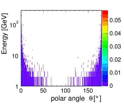
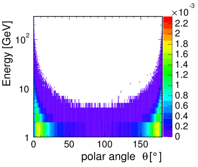
Figure 1: Energy Distribution of the simulated particles from incoherent pair production (left) and from $\mathup{}\mathup{}\rightarrow\mathrm{hadrons}$ processes (right). Both distributions are normalised to unity.

3 Analysis framework

Top pair events were generated using the whizard 1.95 [13, 14] Monte Carlo generator while all other samples were obtained using physsim [15]. The expected luminosity spectrum at the ILC was taken into account during the event generation. The model for the non-perturbative hadronisation in pythia 6.4 [16] with a tune of the hadronisation parameters to opal data was used for all samples.

All events are simulated in the sidloi3 model of the SiD detector concept using slic [18], which is a thin wrapper around geant4 [19, 20]. They are reconstructed by the algorithms in the org.lcsim [21] and slicPandora [22] programs. The LCFIPlus [23] package is used for flavour tagging. The assumed integrated luminosity of the analysis is 1 $\mathrm{ab}^{-1}$ , which is split equally between the two polarisation states $(+80\%,-20\%)$ and $(-80\%,+20\%)$ for the polarization of electron and positron beams $(P_{\mathup{{{\mathup{{{e}}}}}^{\scriptstyle{-}}}},P_{\mathup{{{\mathup{{{e}}}}}^{\scriptstyle{+}}}})$. Background from processes described in Section 2 is overlayed on the hit level before the digitization using a procedure [24] originally developed for CLIC.

4 The sidloi3 detector model

The sidloi3 detector model, in which these studies are carried out, is a general-purpose detector with a 4 $\pi$ coverage as described in the SiD Letter of Intent [25]. It is designed for particle flow calorimetry using highly granular calorimeters.

A superconducting solenoid with an inner radius of 2.6 m provides a central magnetic field of 5 T. The calorimeters are placed inside the coil and consist of a 30 layer tungsten–silicon electromagnetic calorimeter with 13 $\mathrm{mm}^{2}$ segmentation, followed by a hadronic calorimeter with steel absorber and instrumented with resistive plate chambers (RPC) – 40 layers in the barrel region and 45 layers in the endcaps. The read-out cell size in the hadronic calorimeters is $10\times 10$ $\mathrm{mm}^{2}$. The iron return yoke outside of the coil is instrumented with 11 RPC layers with $30\times 30$ $\mathrm{mm}^{2}$ read-out cells for muon identification.

The silicon-only tracking system consists of five $20\times 20$ $\upmu\mathrm{m}^{2}$ pixel layers followed by five strip layers with a pitch of 25 $\upmu\mathrm{m}$, a read-out pitch of 50 $\upmu\mathrm{m}$ and a length of 92 mm in the barrel region. The tracking system in the endcap consists of four stereo-strip disks with similar pitch and a stereo angle of $12^{\circ}$, complemented by four pixelated disks in the vertex region with a pixel size of $20\times 20$ $\upmu\mathrm{m}^{2}$ and three disks in the far-forward region at lower radii with a pixel size of $50\times 50$ $\upmu\mathrm{m}^{2}$. All sub-detectors have time-stamping capability that allow to separate hits originating from different bunch crossings.

5 Analysis strategy and Monte Carlo samples

Figure 2: Diagrams for $\mathup{{{t}}}\mathup{{\overline{{\mathup{{{t}}}}}}}\mathup{{{H}}}$ production in $\mathup{{{\mathup{{{e}}}}}^{\scriptstyle{+}}}\mathup{{{\mathup{{{e}}}}}^{\scriptstyle{-}}}$ collisions.

The measurement of the cross section for the process $\mathup{{{\mathup{{{e}}}}}^{\scriptstyle{+}}}\mathup{{{\mathup{{{e}}}}}^{\scriptstyle{-}}}\to\mathup{{{t}}}\mathup{{\overline{{\mathup{{{t}}}}}}}\mathup{{{H}}}$ using two different final states is described in the following. The Feynman diagrams for this process are shown in Figure 2. Here $\mathup{{{H}}}$ is a Standard Model Higgs boson of mass 125 GeV. The diagram shown on the left represents the dominant contribution to the cross section. This diagram is directly sensitive to the top Yukawa coupling $y_{t}$. The contribution from Higgsstrahlung off the intermediate $\mathup{{{Z}}}$ boson increases the cross section for the $\mathup{{{t}}}\mathup{{\overline{{\mathup{{{t}}}}}}}\mathup{{{H}}}$ final state by about 4% [15]. This represents a small correction which needs to be taken into account in the extraction of $y_{t}$ from the measured cross section. The correction will be known with good precision, because the Higgs coupling to the $\mathup{{{Z}}}$ boson can be extracted from measurements of $\mathup{{{\mathup{{{e}}}}}^{\scriptstyle{+}}}\mathup{{{\mathup{{{e}}}}}^{\scriptstyle{-}}}\to\mathup{{{H}}}\mathup{{{Z}}}$ events at $\sqrt{s}=250\,\mathrm{GeV}$ with a statistical unceratainty of about 1.5% [25, 26].

The measurement of the $\mathup{{{t}}}\mathup{{\overline{{\mathup{{{t}}}}}}}\mathup{{{H}}}$ cross section at the ILC allows a direct extraction of the top Yukawa coupling with good precision. In the analysis presented here, the Higgs decay $\mathup{{{H}}}\to\mathup{{{b}}}\mathup{{\overline{{\mathup{{{b}}}}}}}$ is considered. Two final states are investigated in the following:

• 8 jets: In this case both $\mathup{{{W}}}$ bosons from $\mathup{{{t}}}\mathup{{\overline{{\mathup{{{t}}}}}}}$ decay hadronically. Hence this final state contains eight jets out of which four originate from b-quark decays.

• 6 jets: Here one $\mathup{{{W}}}$ boson decays hadronically and the other $\mathup{{{W}}}$ boson decays leptonically. The final state contains four b-jets, two further jets, an isolated lepton and missing energy. Only electrons and muons are considered as isolated leptons in the final state.

This study requires jet clustering in complex hadronic final states, missing energy reconstruction, flavour-tagging and reconstruction and identification of high energy leptons. Hence it represents a comprehensive check of the complete analysis chain and overall detector performance.

Table 1: Production cross sections times branching ratios or production cross sections for the signal final states and for the considered backgrounds. All samples were generated assuming a Standard Model Higgs with a mass of 125 GeV. The numbers for “other $\mathup{{{t}}}\mathup{{\overline{{\mathup{{{t}}}}}}}\mathup{{{H}}}$” processes in this table do not include either of the signal final states (see text). The $\mathup{{{t}}}\mathup{{\overline{{\mathup{{{t}}}}}}}\mathup{{{Z}}}$ and $\mathup{{{t}}}\mathup{{\overline{{\mathup{{{t}}}}}}}\mathup{{{g}}}^{*}$ samples, where $\mathup{{{g}}}^{*}$ is a hard gluon splitting into a $\mathup{{{b}}}\mathup{{\overline{{\mathup{{{b}}}}}}}$ pair, do not contain events where both top quarks decay leptonically. The $\mathup{{{t}}}\mathup{{\overline{{\mathup{{{t}}}}}}}$ samples contain all possible decays of both $\mathup{{{W}}}$ bosons.

Type	Final state	P($\mathup{{{\mathup{{{e}}}}}^{\scriptstyle{-}}}$)	P($\mathup{{{\mathup{{{e}}}}}^{\scriptstyle{+}}}$)	Cross section [$\times$ BR] (fb)
Signal	$\mathup{{{t}}}\mathup{{\overline{{\mathup{{{t}}}}}}}\mathup{{{H}}}$ (8 jets)	$-80\%$	$+20\%$	0.87
Signal	$\mathup{{{t}}}\mathup{{\overline{{\mathup{{{t}}}}}}}\mathup{{{H}}}$ (8 jets)	$+80\%$	$-20\%$	0.44
Signal	$\mathup{{{t}}}\mathup{{\overline{{\mathup{{{t}}}}}}}\mathup{{{H}}}$ (6 jets)	$-80\%$	$+20\%$	0.84
Signal	$\mathup{{{t}}}\mathup{{\overline{{\mathup{{{t}}}}}}}\mathup{{{H}}}$ (6 jets)	$+80\%$	$-20\%$	0.42
Background	other $\mathup{{{t}}}\mathup{{\overline{{\mathup{{{t}}}}}}}\mathup{{{H}}}$	$-80\%$	$+20\%$	1.59
Background	other $\mathup{{{t}}}\mathup{{\overline{{\mathup{{{t}}}}}}}\mathup{{{H}}}$	$+80\%$	$-20\%$	0.80
Background	$\mathup{{{t}}}\mathup{{\overline{{\mathup{{{t}}}}}}}Z$	$-80\%$	$+20\%$	6.92
Background	$\mathup{{{t}}}\mathup{{\overline{{\mathup{{{t}}}}}}}Z$	$+80\%$	$-20\%$	2.61
Background	$\mathup{{{t}}}\mathup{{\overline{{\mathup{{{t}}}}}}}g^{*}\to\mathup{{{t}}}\mathup{{\overline{{\mathup{{{t}}}}}}}\mathup{{{b}}}\mathup{{\overline{{\mathup{{{b}}}}}}}$	$-80\%$	$+20\%$	1.72
Background	$\mathup{{{t}}}\mathup{{\overline{{\mathup{{{t}}}}}}}g^{*}\to\mathup{{{t}}}\mathup{{\overline{{\mathup{{{t}}}}}}}\mathup{{{b}}}\mathup{{\overline{{\mathup{{{b}}}}}}}$	$+80\%$	$-20\%$	0.86
Background	$\mathup{{{t}}}\mathup{{\overline{{\mathup{{{t}}}}}}}$	$-80\%$	$+20\%$	449
Background	$\mathup{{{t}}}\mathup{{\overline{{\mathup{{{t}}}}}}}$	$+80\%$	$-20\%$	170

An overview of the cross sections for the signal final states as well as for the considered backgrounds is shown in Table 1. For the measurement using the final state with six jets, all other $\mathup{{{t}}}\mathup{{\overline{{\mathup{{{t}}}}}}}\mathup{{{H}}}$ events, i.e., all events where both top quarks decay leptonically or hadronically, or events where the Higgs boson does not decay into $\mathup{{{b}}}\mathup{{\overline{{\mathup{{{b}}}}}}}$, are treated as background. For the eight jets final state events where at least one top quark decays leptonically or where the Higgs boson does not decay into $\mathup{{{b}}}\mathup{{\overline{{\mathup{{{b}}}}}}}$ are considered as background. All non-$\mathup{{{t}}}\mathup{{\overline{{\mathup{{{t}}}}}}}\mathup{{{H}}}$ backgrounds are considered for both measurements.

6 Reconstruction of isolated leptons

The productions cross sections for signal events with six or eight jets in the final state are similar. Signal events with six jets contain one high-energetic isolated lepton from the leptonic $\mathup{{{W}}}$ boson decay. On the other hand, no isolated leptons are expected in signal events with eight jets. Hence the number of isolated leptons is an important observable in the signal selections for both final states. In this study, the isolated electrons or muons are considered.

The IsolatedLeptonFinder processor as implemented in MarlinReco [27] is used to identify leptons in regions with otherwise little calorimetric activity. The identification of isolated leptons starts from charged tracks. First isolation criteria and in a second step identification criteria for electrons and muons based on calorimeter depositions associated to the tracks are applied. These two steps are discussed in the following.

The isolation criteria were optimised on a sample of $\mathup{{{t}}}\mathup{{\overline{{\mathup{{{t}}}}}}}\mathup{{{H}}}$ events with one leptonic $\mathup{{{W}}}$ decay by a parameter scan. A set of parameters yielding a high significance for finding this leptonic $\mathup{{{W}}}$ decay over selecting other lepton candidates is listed in Table 2. This is illustrated in Figure 3, where the energy of particles in a cone around a track, defined by $\cos\theta>0.99$, is plotted versus the track energy in a sample of $\mathup{{{t}}}\mathup{{\overline{{\mathup{{{t}}}}}}}\mathup{{{H}}}$ events with one leptonic $\mathup{{{W}}}$ decay. The cones around tracks that are matched to the $\mathup{{{W}}}$ decay contain generally little additional energy and the data points are concentrated along the x-axis, while other tracks are more likely to be found inside a jet and are therefore found closer to the y- than the x-axis. It is found that a non-linear parametrisation of the relationship between cone energy and track energy improves the performance of the isolated lepton identification.

(a) Track Parameters

Parameter	Value
2D impact parameter $d_{0}$	0.02 mm
z-value of POCA $z_{0}$	0.1 mm
3D impact parameter $r_{0}$	0.1 mm

(b) Parameters of the polynomial energy isolation $E_{\text{cone}}^{2}<AE_{\text{lepton}}^{2}+BE_{\text{lepton}}+C$

cone size	$\cos\theta>0.99$
A	0
B	3.0
C	0

Table 2: Chosen set of parameters to steer the IsolatedLeptonFinder processor in MarlinReco. The point of closest approach (POCA) $z_{0}$ is defined as the smallest distance between the track and the primary vertex along the beam direction.

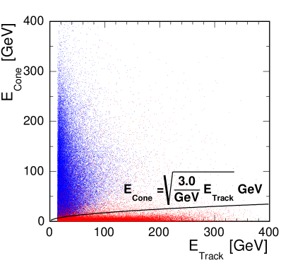
Figure 3: Scatter plot of the energy within a $\cos\theta>0.99$ cone around a track versus the track energy in a sample of $\mathup{{{t}}}\mathup{{\overline{{\mathup{{{t}}}}}}}\mathup{{{H}}}$ events with one leptonic $\mathup{{{W}}}$ decay. Tracks that are matched to the $\mathup{{{W}}}$ decay are shown in red, all other tracks are represented by blue points. Tracks below the black curve in this plot are used as isolated lepton candidates.

The electron and muon identification criteria based on their energy deposition in the ECAL and HCAL were optimised in a separate step. For electrons, the fraction of ECAL to HCAL energy depositions is required to satisfy $0.95<E_{\text{ECAL}}/(E_{\text{ECAL}}+E_{\text{HCAL}})<1$, and the ratio of ECAL energy deposition to track energy meets the requirement $0.85<E_{\text{ECAL}}/p_{\text{track}}<1.15$ (using the pion hypothesis). The requirements on the energy depositions for the selection of muons are $0.03<E_{\text{ECAL}}/(E_{\text{ECAL}}+E_{\text{HCAL}})<0.2$ and $0<E_{\text{ECAL}}/p_{\text{track}}<0.4$.

7 Reconstruction of W, top and Higgs candidates

As a first step of the event analysis chain, isolated leptons are found as described in Sec. 6. The particle flow objects (PFOs) identified as isolated muons or electrons are excluded from the jet reconstruction procedure. Only PFOs in the range $20^{\circ}<\theta<160^{\circ}$ are considered in the following, because the particles originating from the signal processes are located in the central part of the detector while the beam-related backgrounds peak in the forward direction (see Sec. 2). The Durham jet clustering algorithm [28] is used in the exclusive mode with six or eight jets.

To form $\mathup{{{W}}}$, top and Higgs candidates from the reconstructed jets, the following function is minimised for the final state with eight jets:

$$\chi^{2}_{\textnormal{8 jets}}=\frac{(M_{12}-M_{\mathup{{{W}}}})^{2}}{\sigma_{\mathup{{{W}}}}^{2}}+\frac{(M_{123}-M_{\mathup{{{t}}}})^{2}}{\sigma_{\mathup{{{t}}}}^{2}}+\frac{(M_{45}-M_{\mathup{{{W}}}})^{2}}{\sigma_{\mathup{{{W}}}}^{2}}+\frac{(M_{456}-M_{\mathup{{{t}}}})^{2}}{\sigma_{\mathup{{{t}}}}^{2}}+\frac{(M_{78}-M_{\mathup{{{H}}}})^{2}}{\sigma_{\mathup{{{H}}}}^{2}},$$ (2)

where $M_{12}$ and $M_{45}$ are the invariant masses of the jet pairs used to reconstructed the $\mathup{{{W}}}$ candidates, $M_{123}$ and $M_{456}$ are the invariant masses of the three jets used to reconstruct the top candidates and $M_{78}$ is the invariant mass of the jet pair used to reconstruct the Higgs candidate. $M_{\mathup{{{W}}}}$, $M_{t}$ and $M_{\mathup{{{H}}}}$ are the nominal $\mathup{{{W}}}$, top and Higgs masses. The resolutions $\sigma_{\mathup{{{W}}}}$, $\sigma_{\text{t}}$ and $\sigma_{\mathup{{{H}}}}$ were obtained from reconstructed jet combinations matched to $\mathup{{{W}}}$, top and Higgs particles at generator level. The corresponding function minimised for the six jet final state is given by:

$$\chi^{2}_{\textnormal{6 jets}}=\frac{(M_{12}-M_{\mathup{{{W}}}})^{2}}{\sigma_{\mathup{{{W}}}}^{2}}+\frac{(M_{123}-M_{\mathup{{{t}}}})^{2}}{\sigma_{\mathup{{{t}}}}^{2}}+\frac{(M_{45}-M_{\mathup{{{H}}}})^{2}}{\sigma_{\mathup{{{H}}}}^{2}}.$$ (3)

8 Beauty identification

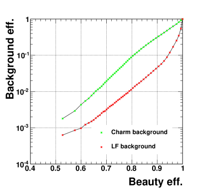
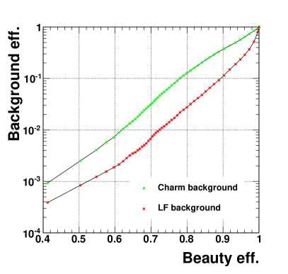
Figure 4: Mis-identification efficiency of light flavour (LF) quark jets (red points) and charm jets (green points) as beauty jets versus beauty identification efficiency in di-jets at $\sqrt{s}=91\,\mathrm{GeV}$. The performance is shown without (left) and with (right) background from $\mathup{}\mathup{}\rightarrow\mathrm{hadrons}$ events and incoherent pairs.

A b-tag value is obtained for each jet reconstructed as described in the section above. To illustrate the flavour tagging performance of the sidloi3 detector, the mis-identification efficiency of light quark (u, d and s) jets or charm jets, respectively, as beauty jets versus the beauty identification efficiency is shown in Figure 4. The mis-identification rates are calculated using di-jet events at a centre-of-mass energy of $91.2\,\mathrm{GeV}$. For this figure, no cut on the polar angles of the PFOs used as input to the jet reconstruction is applied. A sizeable degradation of the flavour tagging performance due to the impact of beam-induced backgrounds is observed. This effect is smaller for the mis-identification of charm jets than for light quark jets.

The training of the flavour tagging for the measurement of $\mathup{{{t}}}\mathup{{\overline{{\mathup{{{t}}}}}}}\mathup{{{H}}}$ production reported in this document is based on events with six quarks of the same flavour produced in electron-positron annihilation. For the training, 60000 charm- and beauty-jets, and 180000 light quark jets are used. These samples were chosen since the jets have similar kinematic properties as those in $\mathup{{{t}}}\mathup{{\overline{{\mathup{{{t}}}}}}}\mathup{{{H}}}$ signal events.

9 Event selection

Events were selected using Boosted Decision Trees (BDTs) as implemented in TMVA [29]. The BDTs were trained separately for the eight and six jet final states. The following input variables were used:

• the four highest b-tag values. The third and fourth highest b-tag value are especially suited to reject $\mathup{{{t}}}\mathup{{\overline{{\mathup{{{t}}}}}}}$ and most of the $\mathup{{{t}}}\mathup{{\overline{{\mathup{{{t}}}}}}}Z$ events which contain only two b-jets;

• the event thrust. Since the top quarks in $\mathup{{{t}}}\mathup{{\overline{{\mathup{{{t}}}}}}}$ events are produced back to back, the thrust variable has larger values in $\mathup{{{t}}}\mathup{{\overline{{\mathup{{{t}}}}}}}$ events compared to $\mathup{{{t}}}\mathup{{\overline{{\mathup{{{t}}}}}}}\mathup{{{H}}}$, $\mathup{{{t}}}\mathup{{\overline{{\mathup{{{t}}}}}}}Z$ or $\mathup{{{t}}}\mathup{{\overline{{\mathup{{{t}}}}}}}\mathup{{{b}}}\mathup{{\overline{{\mathup{{{b}}}}}}}$ events;

• a distance value from the Durham algorithm. The distance parameter between $i$ and $j=(i-1)$ jets is defined as:

  $$Y_{ij}=\frac{\min(E_{m}^{2},E_{n}^{2})(1-\cos\theta_{mn})}{s},$$ (4)

  where $m$ and $n$ are chosen to minimise the distance of the two jets which are merged. If more jets are reconstructed than coloured final state partons are present in an event, the distance parameter tends to small values. For the six jet final state $Y_{65}$ is used while $Y_{87}$ is used for the eight jet final state;

• the number of reconstructed PFOs in the range $20^{\circ}<\theta<160^{\circ}$;

• the number of identified isolated electrons and muons;

• the missing transverse momentum, $p_{\mathrm{T}}^{\textnormal{miss}}$, calculated from the reconstructed jets. Due to the leptonic $\mathup{{{W}}}$ boson decay, finite values of $p_{\mathrm{T}}^{\textnormal{miss}}$ are reconstructed for six jet signal events while $p_{\mathrm{T}}^{\textnormal{miss}}$ tends towards zero for eight jet signal events;

• the total visible energy defined as the scalar sum of all jet energies;

• the masses $M_{12}$, $M_{123}$ and $M_{45}$ as defined in Section 7.

For the eight jet final state two additional variables are included:

• $M_{456}$ and $M_{78}$ as defined in Section 7.

The distributions of all input variables are shown in Appendix A for the six jet final state and in Appendix B for the eight jet final state.

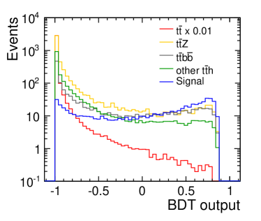
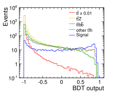
Figure 5: Output distributions of the BDTs for the eight (left) and six (right) jet final states. The signals are shown in blue while the backgrounds are shown in different colours. The distribution for $\mathup{{{t}}}\mathup{{\overline{{\mathup{{{t}}}}}}}$ was scaled by a factor of $0.01$.

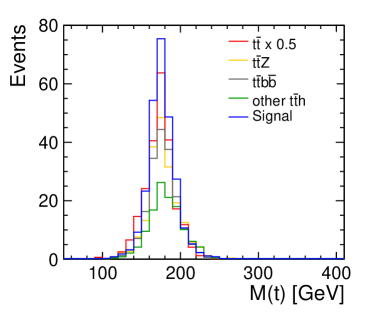
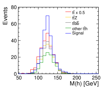
Figure 6: Reconstructed top (left) and Higgs (right) masses for the selected (BDT output value $>$ 0.1978) six jet events. The signal is shown in blue while the backgrounds are shown in different colours. The distribution for $\mathup{{{t}}}\mathup{{\overline{{\mathup{{{t}}}}}}}$ was scaled by a factor of $0.5$.

The output values of the BDTs for the signals and for the different backgrounds are shown in Figure 5 for both final states. To select events, cuts on the BDT output values are applied. The cuts were optimised by maximising the signal significance given by: $\frac{S}{\sqrt{S+B}}$, where $S$ is the number of signal events and $B$ is the number of background events. As an example, the reconstructed top and Higgs masses in six jet events after the cut on the BDT output are shown in Figure 6. The selection efficiencies for signal events are 42% and 54% for the six and eight jet final states, respectively. In Table 3 the numbers of events passing the cuts on the BDT output values are shown separately for all investigated final states.

Table 3: Number of selected events for the different final states assuming an integrated luminosity of 1 $\mathrm{ab}^{-1}$. The values obtained for the six and eight jet final state selections are shown separately.

Final state	BDT trained to select 6 jets	BDT trained to select 8 jets
$\mathup{{{t}}}\mathup{{\overline{{\mathup{{{t}}}}}}}\mathup{{{H}}}$, $\mathup{{{H}}}\to\mathup{{{b}}}\mathup{{\overline{{\mathup{{{b}}}}}}}$ (6 jets)	264.9	87.2
$\mathup{{{t}}}\mathup{{\overline{{\mathup{{{t}}}}}}}\mathup{{{H}}}$, $\mathup{{{H}}}\to\mathup{{{b}}}\mathup{{\overline{{\mathup{{{b}}}}}}}$ (8 jets)	72.6	356.2
$\mathup{{{t}}}\mathup{{\overline{{\mathup{{{t}}}}}}}\mathup{{{H}}}$, $\mathup{{{H}}}$ not $\mathup{{{b}}}\mathup{{\overline{{\mathup{{{b}}}}}}}$ (6 jets)	11.7	5.1
$\mathup{{{t}}}\mathup{{\overline{{\mathup{{{t}}}}}}}\mathup{{{H}}}$, $\mathup{{{H}}}$ not $\mathup{{{b}}}\mathup{{\overline{{\mathup{{{b}}}}}}}$ (8 jets)	4.3	21.6
$\mathup{{{t}}}\mathup{{\overline{{\mathup{{{t}}}}}}}\mathup{{{H}}}$ (4 jets)	32.8	2.1
$\mathup{{{t}}}\mathup{{\overline{{\mathup{{{t}}}}}}}Z$	188.4	253.6
$\mathup{{{t}}}\mathup{{\overline{{\mathup{{{t}}}}}}}g^{*}\to\mathup{{{t}}}\mathup{{\overline{{\mathup{{{t}}}}}}}\mathup{{{b}}}\mathup{{\overline{{\mathup{{{b}}}}}}}$	185.0	243.6
$\mathup{{{t}}}\mathup{{\overline{{\mathup{{{t}}}}}}}$	459.3	687.0

10 Results

The cross section can be directly obtained from the number of background-subtracted signal events after the selection. The uncertainty of the cross section measurement was estimated using the number of selected signal and background events. Assuming an integrated luminosity of 1 $\mathrm{ab}^{-1}$ split equally between the $P(\mathup{{{\mathup{{{e}}}}}^{\scriptstyle{-}}})=-80\%$, $P(\mathup{{{\mathup{{{e}}}}}^{\scriptstyle{+}}})=+20\%$ and $P(\mathup{{{\mathup{{{e}}}}}^{\scriptstyle{-}}})=+80\%$, $P(\mathup{{{\mathup{{{e}}}}}^{\scriptstyle{+}}})=-20\%$ beam polarisaiton configurations, the cross section can be measured with a statistical accuracy of $11.5\%$ using the eight jet final state and with a statistical accuracy of $13.2\%$ for the six jet final state.

As a cross check, the analysis was repeated preselecting events with one isolated lepton for the six jet final state and events without isolated leptons for the eight jet final state. In Appendix C the numbers of selected events are shown for this approach. The differences in precision on the top Yukawa coupling compared to the nominal analysis are negligible.

To extract the top Yukawa coupling from the measured cross sections, signal Monte Carlo samples with different values of the top Yukawa coupling were generated. The dependence of the cross section on the value of the coupling was fitted using a quadratic function. The following relation was found: $\frac{\Delta y_{\mathup{{{t}}}}}{y_{\mathup{{{t}}}}}=0.52\cdot\frac{\Delta\sigma}{\sigma}$ [30]. The factor between the cross section uncertainty and the coupling uncertainty differs from $0.5$ due to the contribution from Higgsstrahlung to the $\mathup{{{t}}}\mathup{{\overline{{\mathup{{{t}}}}}}}\mathup{{{H}}}$ production cross section. The uncertainties of the measured cross sections translate to precisions on the top Yukawa coupling of $6.0\%$ and $6.9\%$ from the eight and six jet final states, respectively. If both measurements are combined, the top Yukawa coupling can be extracted with a statistical accuracy of $4.5\%$. Good agreement with a similar study performed using the ILD detector concept [30] is observed.

For 1 $\mathrm{ab}^{-1}$ of data with only $P(\mathup{{{\mathup{{{e}}}}}^{\scriptstyle{-}}})=-80\%$, $P(\mathup{{{\mathup{{{e}}}}}^{\scriptstyle{+}}})=+20\%$ polarisation, this number improves to $4.0\%$.

The precision for the six jet final state could be improved further if $\tau$-leptons were included in the reconstruction. Additional improvements of the analysis procedure like kinematic fitting will be investigated in the future.

The uncertainty on BR($\mathup{{{H}}}\to\mathup{{{b}}}\mathup{{\overline{{\mathup{{{b}}}}}}}$) is neglected in the calculation of the top Yukawa coupling from the $\mathup{{{t}}}\mathup{{\overline{{\mathup{{{t}}}}}}}\mathup{{{H}}}$ production cross section, because it is expected that this quantity can be measured with a precision of better than $1\%$ using $\mathup{{{\mathup{{{e}}}}}^{\scriptstyle{+}}}\mathup{{{\mathup{{{e}}}}}^{\scriptstyle{-}}}\to\mathup{}\mathup{{\overline{{\upnu}}}}\mathup{{{H}}}$ events [31, 32].

Systematic uncertainties were not investigated in detail so far. However, it is expected that the relevant sources of systematic uncertainty like the beauty identification, the jet energy scale or the knowledge of the luminosity spectrum will result in errors that are small compared to the statistical precision of the measurements. The understanding of the detector acceptances can be checked using processes like $\mathup{{{t}}}\mathup{{\overline{{\mathup{{{t}}}}}}}$ or $\mathup{{{t}}}\mathup{{\overline{{\mathup{{{t}}}}}}}Z$ where the cross sections can be predicted precisely.

11 Summary

The physics potential for a measurement of the top Yukawa coupling at 1 TeV using the SiD detector is investigated. The study is based on a full detector simulation. Beam-induced backgrounds are considered in the analysis. The combination of results obtained for two different final states leads to a statistical uncertainty on the top Yukawa coupling of $4.5\%$ for an integrated luminosity of 0.5 $\mathrm{ab}^{-1}$ with the $P(\mathup{{{\mathup{{{e}}}}}^{\scriptstyle{-}}})=-80\%$, $P(\mathup{{{\mathup{{{e}}}}}^{\scriptstyle{+}}})=+20\%$ beam polarisation configuration and 0.5 $\mathrm{ab}^{-1}$ with $P(\mathup{{{\mathup{{{e}}}}}^{\scriptstyle{-}}})=+80\%$, $P(\mathup{{{\mathup{{{e}}}}}^{\scriptstyle{+}}})=-20\%$ polarisation.

12 Acknowledgements

The authors would like to thank Tim Barklow, Mikael Berggren and Akiya Miyamoto for generating the Monte Carlo samples. We gratefully acknowlege the help from Christian Grefe and Stephane Poss with the production on the Grid. Finally, we wish to thank Tony Prince and Tomohiko Tanabe for comparisons of the results to the ILD analysis.

Appendix A Control plots for the six jet final state

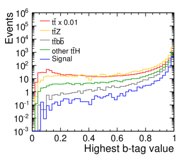
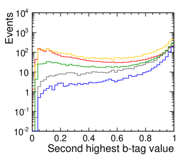
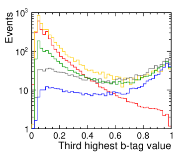
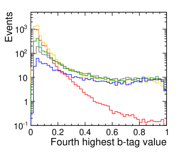
Figure 7: Distributions of several discriminating variables used in the event selection for the six jet final state. The signals are shown in blue while the backgrounds are shown in different colours. The distribution for $\mathup{{{t}}}\mathup{{\overline{{\mathup{{{t}}}}}}}$ was scaled by a factor of $0.01$.

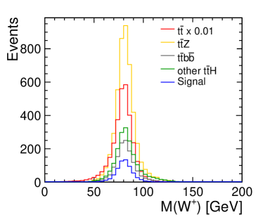
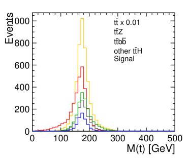
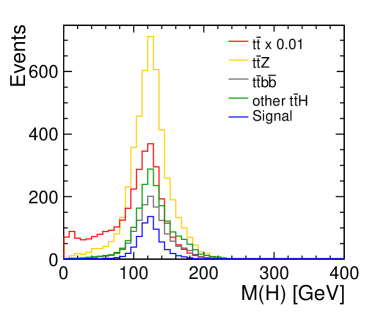
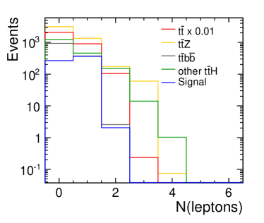
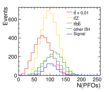
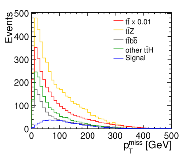
Figure 8: Distributions of several discriminating variables used in the event selection for the six jet final state. The signals are shown in blue while the backgrounds are shown in different colours. The distribution for $\mathup{{{t}}}\mathup{{\overline{{\mathup{{{t}}}}}}}$ was scaled by a factor of $0.01$.

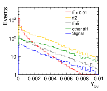
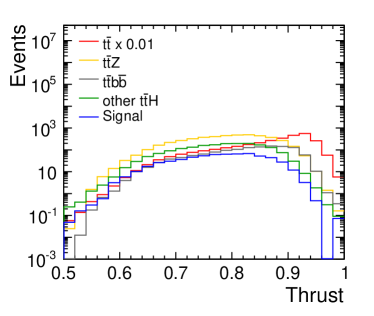
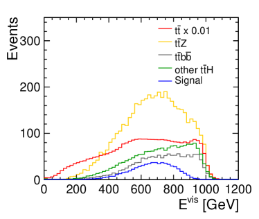
Figure 9: Distributions of several discriminating variables used in the event selection for the six jet final state. The signals are shown in blue while the backgrounds are shown in different colours. The distribution for $\mathup{{{t}}}\mathup{{\overline{{\mathup{{{t}}}}}}}$ was scaled by a factor of $0.01$.

Appendix B Control plots for the eight jet final state

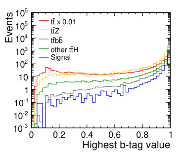
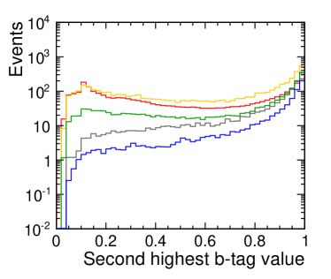
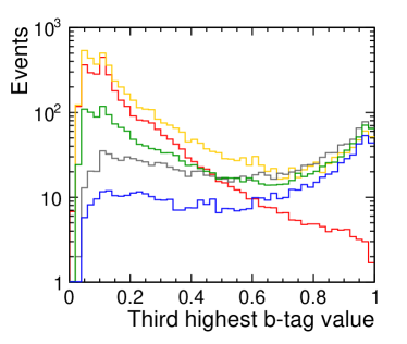
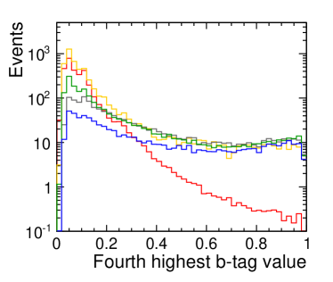
Figure 10: Distributions of several discriminating variables used in the event selection for the eight jet final state. The signals are shown in blue while the backgrounds are shown in different colours. The distribution for $\mathup{{{t}}}\mathup{{\overline{{\mathup{{{t}}}}}}}$ was scaled by a factor of $0.01$.

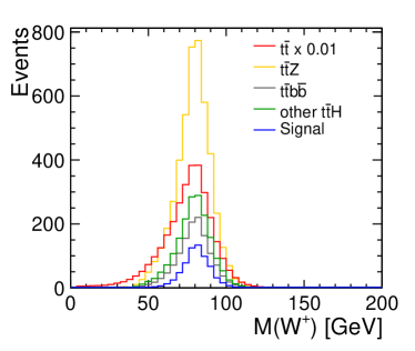
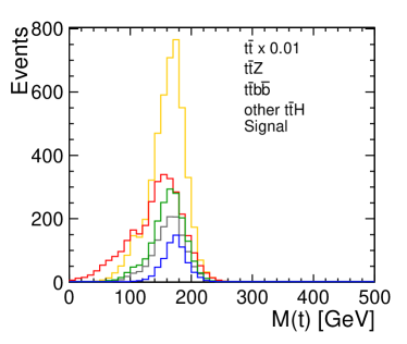
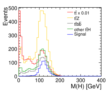
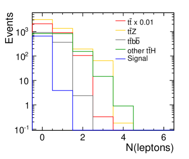
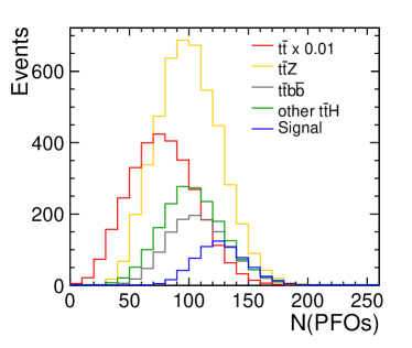
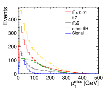
Figure 11: Distributions of several discriminating variables used in the event selection for the eight jet final state. The signals are shown in blue while the backgrounds are shown in different colours. The distribution for $\mathup{{{t}}}\mathup{{\overline{{\mathup{{{t}}}}}}}$ was scaled by a factor of $0.01$.

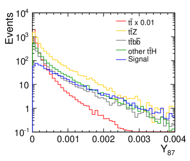
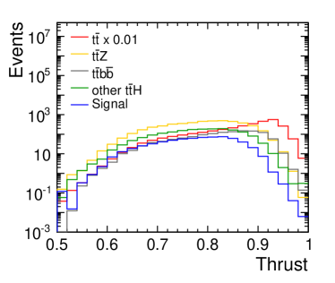
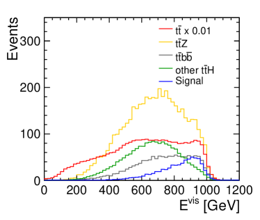
Figure 12: Distributions of several discriminating variables used in the event selection for the eight jet final state. The signals are shown in blue while the backgrounds are shown in different colours. The distribution for $\mathup{{{t}}}\mathup{{\overline{{\mathup{{{t}}}}}}}$ was scaled by a factor of $0.01$.

Appendix C Number of selected events with preselection on the number of isolated leptons

Table 4: Number of selected events for the different final states assuming an integrated luminosity of 1 $\mathrm{ab}^{-1}$. The values obtained for the six and eight jet final state selections are shown separately. Events with one isolated lepton are preselected for the six jet final state and events without isolated leptons are preselected for the eight jet final state before the training of the BDTs.

Final state	BDT trained to select 6 jets	BDT trained to select 8 jets
$\mathup{{{t}}}\mathup{{\overline{{\mathup{{{t}}}}}}}\mathup{{{H}}}$, $\mathup{{{H}}}\to\mathup{{{b}}}\mathup{{\overline{{\mathup{{{b}}}}}}}$ (6 jets)	191.6	57.4
$\mathup{{{t}}}\mathup{{\overline{{\mathup{{{t}}}}}}}\mathup{{{H}}}$, $\mathup{{{H}}}\to\mathup{{{b}}}\mathup{{\overline{{\mathup{{{b}}}}}}}$ (8 jets)	1.6	299.4
$\mathup{{{t}}}\mathup{{\overline{{\mathup{{{t}}}}}}}\mathup{{{H}}}$, $\mathup{{{H}}}$ not $\mathup{{{b}}}\mathup{{\overline{{\mathup{{{b}}}}}}}$ (6 jets)	9.6	2.8
$\mathup{{{t}}}\mathup{{\overline{{\mathup{{{t}}}}}}}\mathup{{{H}}}$, $\mathup{{{H}}}$ not $\mathup{{{b}}}\mathup{{\overline{{\mathup{{{b}}}}}}}$ (8 jets)	2.5	12.4
$\mathup{{{t}}}\mathup{{\overline{{\mathup{{{t}}}}}}}\mathup{{{H}}}$ (4 jets)	20.9	1.4
$\mathup{{{t}}}\mathup{{\overline{{\mathup{{{t}}}}}}}Z$	105.6	187.1
$\mathup{{{t}}}\mathup{{\overline{{\mathup{{{t}}}}}}}g^{*}\to\mathup{{{t}}}\mathup{{\overline{{\mathup{{{t}}}}}}}\mathup{{{b}}}\mathup{{\overline{{\mathup{{{b}}}}}}}$	100.1	180.7
$\mathup{{{t}}}\mathup{{\overline{{\mathup{{{t}}}}}}}$	232.0	381.6

References

- [1] S. Chatrchyan et al., Observation of a new boson at a mass of 125 GeV with the CMS experiment at the LHC, Phys. Lett. B 716 (2012) 30–61
- [2] G. Aad et al., Observation of a new particle in the search for the Standard Model Higgs boson with the ATLAS detector at the LHC, Phys. Lett. B 716 (2012) 1–29
- [3] R. S. Gupta, H. Rzehak and J. D. Wells, How well do we need to measure Higgs boson couplings?, Phys. Rev. D 86 (2012) 095001
- [4] J. Brau et al., ILC Reference Design Report: ILC Global Design Effort and World Wide Study (2007), physics.acc-ph/0712.1950
- [5] T. Behnke et al., The International Linear Collider Technical Design Report - Volume 4: Detectors (2013), physics.ins-det/1306.6329
- [6] K. Hagiwara, H. Murayama and I. Watanabe, Search for the Yukawa interaction in the process at TeV linear colliders, Nucl. Phys. B 367 (1991) 257 – 286
- [7] A. Djouadi, J. Kalinowski and P. Zerwas, Measuring the coupling in collisions, Mod. Phys. Lett. A 07 (1992) 1765–1769
- [8] A. Juste and G. Merino, Top Higgs-Yukawa coupling measurement at a linear collider (1999), hep-ph/9910301
- [9] A. Gay, Measurement of the top-Higgs Yukawa coupling at a Linear Collider, Eur. Phys. J. C 49 (2007) 489–497, hep-ph/0604034
- [10] H. Baer, S. Dawson and L. Reina, Measuring the top quark yukawa coupling at a linear collider, Phys. Rev. D 61 (1999) 013002
- [11] R. Yonamine et al., Measuring the top Yukawa coupling at the ILC at , Phys. Rev. D 84 (2011) 014033
- [12] C. Grefe, Occupancies from Beam-Related Backgrounds in SiD for the DBD (2013), presentation given at the SiD Workshop at SLAC
- [13] W. Kilian, T. Ohl and J. Reuter, WHIZARD: Simulating Multi-Particle Processes at LHC and ILC, Eur. Phys. J. C 71 (2011) 1742
- [14] M. Moretti, T. Ohl and J. Reuter, O’Mega: An Optimizing matrix element generator (2001), hep-ph/0102195
- [15] Physics Study Libraries, Website: http://www-jlc.kek.jp/subg/offl/physsim/
- [16] T. Sjostrand, S. Mrenna and P. Z. Skands, PYTHIA 6.4 Physics and Manual, JHEP 05 (2006) 026, hep-ph/0603175
- [17] L. Linssen et al., Physics and Detectors at CLIC: CLIC Conceptual Design Report, CERN 2012-003, 2012
- [18] N. Graf and J. McCormick, Simulator for the linear collider (SLIC): A tool for ILC detector simulations, AIP Conf. Proc. 867 (2006) 503–512
- [19] S. Agostinelli et al., Geant4 – a simulation toolkit, Nucl. Instrum. Meth. Phys. Res. A 506 (2003) 250–303
- [20] J. Allison et al., Geant4 developments and applications, IEEE T. Nucl. Sci. 53 (2006) 270–278
- [21] Linear Collider simulations, http://lcsim.org/software/lcsim/1.18/
- [22] M. A. Thomson, Particle Flow Calorimetry and the PandoraPFA Algorithm, Nucl. Instrum. Meth. A 611 (2009) 25–40
- [23] LCFIPlus, https://confluence.slac.stanford.edu/display/ilc/LCFIPlus
- [24] C. Grefe, OverlayDriver: An event mixing tool for org.lcsim, LCD-Note 2011-032, CERN, 2011
- [25] H. Aihara et al., SiD Letter of Intent (2009), SLAC-R 989
- [26] J. E. Brau et al., The Physics Case for an Linear Collider (2012), hep-ex/1210.0202
- [27] MarlinReco, Website: http://ilcsoft.desy.de/portal/software_packages/marlinreco/
- [28] S. Catani et al., New clustering algorithm for multijet cross sections in annihilation, Phys. Lett. B 269 (1991) 432 – 438
- [29] A. Hoecker et al., TMVA - Toolkit for Multivariate Data Analysis, POSACAT 040 (2007)
- [30] T. Price et al., Measurement of the top Yukawa coupling at using the ILC detector, LC-REP 2013-004, 2013
- [31] T. L. Barklow, Higgs coupling measurements at a 1 TeV linear collider (2003), hep-ph/0312268
- [32] H. Ono, Higgs branching ratio study for DBD detector benchmarking in ILD, LC-REP 2013-005, 2013