Multimode model for an atomic Bose-Einstein condensate in a ring-shaped optical lattice

Abstract

We study the population dynamics of a ring-shaped optical lattice with a high number of particles per site and a low, below ten, number of wells. Using a localized on-site basis defined in terms of stationary states, we were able to construct a multiple-mode model depending on relevant hopping and on-site energy parameters. We show that in case of two wells, our model corresponds exactly to the latest improvement of the two-mode model. We derive a formula for the self-trapping period, which turns out to be chiefly ruled by the on-site interaction energy parameter. By comparing to time dependent Gross-Pitaevskii simulations, we show that the multimode model results can be enhanced in a remarkable way over all the regimes by only renormalizing such a parameter. Finally, using a different approach which involves only the ground state density, we derive an effective interaction energy parameter that shows to be in accordance with the renormalized one.

I Introduction

The two-mode model applied to double-well atomic Bose-Einstein condensates has been extensively studied in the last years Smerzi et al. (1997); Raghavan et al. (1999); Ananikian and Bergeman (2006); Xin Yan Jia et al. (2008); Albiez et al. (2005); Melé-Messeguer et al. (2011); Abad et al. (2011a); Mayteevarunyoo et al. (2008); *xiong; *zhou; *cui; *gui; Jezek et al. (2013); *cond Assuming that the order parameter can be described as a superposition of localized on-site wave functions with time dependent coefficients, such a model predicts Josephson and self-trapping regimes Smerzi et al. (1997); Raghavan et al. (1999), which have been experimentally observed by Albiez et al. Albiez et al. (2005).

The self-trapping (ST) phenomenon, which is also present in extended optical lattices Creffield (2007); *xue; *alex; *fu, is a non linear effect where an initially highly populated (over a critical value) site, remains with a larger number of particles than the remaining sites over all the evolution. There is nowadays an active research on the self-trapping effect, which involves different types of systems, including mixtures of atomic species Kolovsky (2010); *Adhi.

The dynamics of ring-shaped optical lattices with three Viscondi and Furuya (2011) and four wells S. De Liberato and Foot (2006), has been previously investigated through multiple-mode (MM) models which utilized ad-hoc values for hopping and on-site energy parameters. In the present article instead, we will extract such parameters from a mean-field approach using localized on-site functions. We have shown in a previous work Cataldo and Jezek (2011) that in a ring-shaped optical lattice, localized on-site (which we called ‘Wannier-like’ (WL)) functions can be obtained in terms of stationary states of the Gross-Pitaevskii (GP) equation with different winding numbers. Here we will show that the above parameters yield the same type of corrections to the MM model for large filling factors, as those obtained for the improved two-mode (TM) model for two-well systems Ananikian and Bergeman (2006).

We will derive an approximate formula for the self-trapping period in terms of the on-site interaction energy parameter. Using this formula and a single GP simulation results, a renormalizing on-site energy parameter that substantially improves the MM model can be obtained, in what will be called the renormalized multiple-mode (RMM) model. Taking into account the density deformation during the time evolution Smerzi and Trombettoni (2003), it has been shown in a recent work that for a double-well system an effective interaction energy parameter should be considered in the TM model to properly describe the exact dynamics Jezek et al. (2013); *cond. Here we will adapt the same approach to our multiple-well system, which will allow us to obtain such an effective parameter only in terms of the ground state density. Finally, we will show that both approaches give similar results.

This paper is organized as follows. In Sec. II we describe the system and in Sec. III we outline the method for obtaining the WL functions, along with the properties required for building a reasonable multimode model dynamics. There we also define the model parameters in terms of the WL functions. In Sec. IV we specialize to the case of two wells, showing that our treatment through the WL functions turns out to be exactly the same as the latest two-mode model formulation Ananikian and Bergeman (2006). Next, by means of the formula derived for the ST period, we show that the two-mode model can be enhanced in a remarkable way by only renormalizing the on-site interaction energy parameter. In Sec. V we develop the multiple-mode model, which generalizes our finding of the previous section. Finally, based on the method described in Ref. Jezek et al. (2013); *cond, in Sec. VI we derive an effective interaction energy parameter and compare it with the renormalized one. To conclude, a summary of our work is presented in Sec. VII.

II Ring-shaped lattice and condensate parameters

We consider a Bose-Einstein condensate of Rubidium atoms confined by an external trap $V_{\text{trap}}$, consisting of a superposition of a toroidal term $V_{\text{toro}}$ and a lattice potential $V_{\text{L}}(x,y)$ formed by radial barriers. Similarly to the trap utilized in recent experiments Ryu et al. (2007); Weiler et al. (2008), the toroidal trapping potential in cylindrical coordinates reads,

$$V_{\text{toro}}(r,z)=\frac{m}{2}\left[\omega_{r}^{2}r^{2}+\omega_{z}^{2}z^{2}\right]+V_{0}\,\exp(-2\,r^{2}/\;\lambda_{0}^{2})$$ (1)

where $m$ is the atom mass and $\omega_{r}$ and $\omega_{z}$ denote the radial and axial frequencies, respectively. We have set $\omega_{z}>>\omega_{r}$ to suppress excitation in the $z$ direction. In particular, we have chosen $\omega_{r}/(2\pi)=7.8$ Hz and $\omega_{z}/(2\pi)=173$ Hz, while for the laser beam we have set $V_{0}=100\,\hbar\omega_{r}$ and $\lambda_{0}=6\,l_{r}$, with $l_{r}=\sqrt{\hbar/(m\omega_{r})}$. On the other hand, the lattice potential is formed by $N_{c}$ Gaussian barriers located at equally spaced angular positions $\theta_{k}=2\pi k/N_{c}$, where $-[[(N_{c}-1)/2]]\leq k\leq[[N_{c}/2]]$ with $[[.]]$ denoting the integer part,

$$V_{\text{L}}(x,y)=V_{b}\,\,\sum_{k=-[[(N_{c}-1)/2]]}^{[[N_{c}/2]]}\exp\left\{-\frac{[\cos(\theta_{k})\,y-\sin(\theta_{k})\,x]^{2}}{\lambda_{b}^{2}}\right\}\Theta[\sin(\theta_{k})y+\cos(\theta_{k})x],$$ (2)

where $\Theta$ denotes the Heaviside function. For the numerical calculations we have fixed the width of the Gaussians to $\lambda_{b}=0.5\,l_{r}$ and the barrier height to $V_{b}=80\,\hbar\omega_{r}$. In the mean-field approximation, the stationary states are solutions of the GP equation Gross (1961); *pita

$$\left[-\frac{\hbar^{2}}{2m}{\bf\nabla}^{2}+V_{\rm{trap}}({\bf r})+g\,N|\psi_{n}({\bf r})|^{2}\right]\psi_{n}({\bf r})=\mu\,\psi_{n}({\bf r}),$$ (3)

where $\psi_{n}({\bf r})$ denotes a two-dimensional (2D) order parameter Castin and Dum (1999) normalized to unity with winding number $n$ Jezek and Cataldo (2011). The vorticity is numerically imprinted following the procedure described in Ref. Jezek et al. (2008). $N$ and $\mu$ denote, respectively, the number of particles and the chemical potential ($N=10^{5}$ will be assumed over all the numerical calculations). The effective 2D coupling constant $g=g_{3D}\sqrt{m\omega_{z}/2\pi\hbar}$ is written in terms of the 3D coupling constant between the atoms $g_{3D}=4\pi a\hbar^{2}/m$, where $a=98.98\,a_{0}$ denotes the $s$-wave scattering length of ⁸⁷Rb, $a_{0}$ being the Bohr radius. Technical advances have been recently achieved, to obtain experimentally this type of condensates in ring-shaped optical lattices with an arbitrary number of sites Henderson et al. (2009).

III Localized states and hopping and on-site energy parameters

In this section we will summarize the results obtained in a previous work Cataldo and Jezek (2011) that will be used to describe the present dynamics. We are interested in studying the Josephson and ST regimes. Such a dynamics takes place when the ground-state chemical potential becomes smaller than the minimum of the effective potential barrier dividing two lattice sites Jezek and Cataldo (2011).

III.1 Localized WL states

The stationary states $\psi_{n}(r,\theta)$ are obtained as the numerical solutions of Eq. (3) Jezek and Cataldo (2011). Assuming large barrier heights Cataldo and Jezek (2011), the winding number $n$ will be restricted to the values $-[[(N_{c}-1)/2]]\leq n\leq[[N_{c}/2]]$ Jezek and Cataldo (2011). We have seen in Ref. Cataldo and Jezek (2011) that stationary states of different winding number must be orthogonal, and that the following definition for the WL functions

$$w_{k}({r,\theta})=\frac{1}{\sqrt{N_{c}}}\sum_{n}\psi_{n}({r,\theta})\,e^{-in\theta_{k}}\,,$$ (4)

corresponds indeed to well localized functions on each $k$-site. In addition, it has been shown in Ref. Cataldo and Jezek (2011) that the above orthogonality implies that the set of $N_{c}$ WL functions (4) located at different $k$-sites, must also form an orthonormal set. In Fig. 1 we have depicted the WL function density $w_{0}^{2}$ for several values of $N_{c}$, where it becomes clear that they are certainly well-localized functions. Here it is important to recall that the main difference between our WL function and a ‘true’ Wannier function consists in that only the former depends on the filling factor, i.e. the number of particles at each site, as seen in Ref. Cataldo and Jezek (2011).

Figure 1: Density isocontours of the ground-state wave function $|\psi_{0}|^{2}$ for $N_{c}=8$ (a), and of the WL function $w_{0}^{2}({\mathbf{r}})$ for the following numbers of sites $N_{c}=8$ (b), $N_{c}=4$ (c), and $N_{c}=2$ (d).

One may also write the above stationary states in terms of these localized functions,

$$\psi_{n}({\mathbf{r}})=\frac{1}{\sqrt{N_{c}}}\sum_{k}w_{k}({r,\theta})\,e^{in\theta_{k}}\,,$$ (5)

which will be useful to describe the dynamics we are interested in.

III.2 Hopping and on-site energy parameters

The $N_{c}$-mode dynamics will be described in terms of the following parameters,

$$\varepsilon=\int d^{2}{\bf r}\,\,w_{0}(r,\theta)\left[-\frac{\hbar^{2}}{2m}{\bf\nabla}^{2}+V_{\rm{trap}}({\bf r})\right]w_{0}(r,\theta)$$ (6)

$$J=-\int d^{2}{\bf r}\,\,w_{0}(r,\theta)\left[-\frac{\hbar^{2}}{2m}{\bf\nabla}^{2}+V_{\rm{trap}}({\bf r})\right]w_{1}(r,\theta)$$ (7)

$$J^{\prime}=-2\,g\int d^{2}{\bf r}\,\,w_{0}^{3}(r,\theta)\,w_{1}(r,\theta)$$ (8)

$$U=g\int d^{2}{\bf r}\,\,w_{0}^{4}(r,\theta),$$ (9)

which due to the symmetry of the lattice can be written without loss of generality only in terms of the $k=0$ and $k=1$ sites. We want to mention that these parameters can also be efficiently evaluated through the alternative formulae given in Ref. Cataldo and Jezek (2011).

IV Two-mode dynamical equations

When the trapping potential consists of a double well, the condensate dynamics may be simply described through a pair of coupled equations, which corresponds to the two-mode model. Such a TM dynamics has been extensively studied in recent years Raghavan et al. (1999). Particularly, an improved version of this model Ananikian and Bergeman (2006) has been also applied to particles exhibiting a dipolar interaction, which generates self-induced Josephson junctions in a similar toroidal geometry Abad et al. (2011a).

IV.1 Dynamical equations in terms of the coefficients of well-localized functions

The commonly used ansatz for the TM wave function reads

$$\psi_{\rm TM}(r,\theta,t)=b_{R}(t)\,\psi_{R}(r,\theta)+b_{L}(t)\,\psi_{L}(r,\theta),$$ (10)

where $\psi_{R}(r,\theta)$ and $\psi_{L}(r,\theta)$ are well-localized functions at the right and left well, respectively. Such wave functions are easily identified with the WL functions, namely $\psi_{R}(r,\theta)=w_{0}(r,\theta)$ and $\psi_{L}(r,\theta)=w_{1}(r,\theta)$, since from Eq. (4) we get for $N_{c}=2$,

$$w_{0}({r,\theta})=\frac{1}{\sqrt{2}}(\psi_{0}({r,\theta})+\psi_{1}({r,\theta}))\,,$$ (11)

$$w_{1}({r,\theta})=\frac{1}{\sqrt{2}}(\psi_{0}({r,\theta})-\psi_{1}({r,\theta}))\,,$$ (12)

which turns out to be identical to the standard TM variational proposal Smerzi et al. (1997).

Note that the first excited state is an odd function of $x$, as required by the TM model (antisymmetric solution). This can be easily verified by noting that the stationary state with winding number $n=1$ has uniform phases at the right and left well with values $\phi=0$ and $\phi=\pi$, respectively Jezek and Cataldo (2011). Here we may recall that this only occurs in the regime of large barriers Cataldo and Jezek (2011), where $\psi_{1}({\mathbf{r}})=\psi_{-1}({\mathbf{r}})$ may be taken as a real function that does not carry any angular momentum, and hence does not correspond to a ‘vortex’ state Jezek and Cataldo (2011).

In order to obtain the TM equations, we may replace the following order parameter, which is written in terms of the WL functions according to the ansatz (10),

$$\psi_{\rm TM}(r,\theta,t)=b_{0}(t)\,w_{0}(r,\theta)+b_{1}(t)\,w_{1}(r,\theta)\,,$$ (13)

in the time dependent GP equation,

$$i\hbar\frac{\partial\psi_{\rm TM}(r,\theta,t)}{\partial t}=\left[-\frac{\hbar^{2}}{2m}{\bf\nabla}^{2}+V_{\rm{trap}}(r,\theta)+g\,N|\psi_{\rm TM}(r,\theta,t)|^{2}\right]\psi_{\rm TM}(r,\theta,t)\,.$$ (14)

Making use of the orthonormality of the WL functions and recalling the definitions of hopping and on-site energy parameters (Eqs. (6) to (9)) one obtains,

$$i\hbar\,\frac{db_{0}}{dt}=\varepsilon b_{0}-Jb_{1}+UN|b_{0}|^{2}b_{0}-\frac{J^{\prime}}{2}N\,[2{\rm Re}(b_{0}^{*}b_{1})b_{0}+b_{1}],$$ (15)

$$i\hbar\,\frac{db_{1}}{dt}=\varepsilon b_{1}-Jb_{0}+UN|b_{1}|^{2}b_{1}-\frac{J^{\prime}}{2}N\,[2{\rm Re}(b_{1}^{*}b_{0})b_{1}+b_{0}].$$ (16)

The above equations correspond to the improved TM model developed in Ref. Ananikian and Bergeman (2006) and applied in Refs. Melé-Messeguer et al. (2011); Abad et al. (2011a). Here it is worth noticing that we have disregarded in our derivation terms of the order of the following integral

$$I=gN\int d^{2}{\bf r}\,\,w_{0}^{2}(r,\theta)\,w_{1}^{2}(r,\theta),$$ (17)

since the corresponding contributions have been shown to be negligible, as also been argued in Ref. Ananikian and Bergeman (2006) for high barriers.

IV.2 Dynamical equations in terms of the particle imbalance and phase difference

A more convenient set of variables is obtained by observing that $b_{k}(t)=|b_{k}(t)|e^{i\phi_{k}(t)}$, where $\phi_{k}(t)$ is the uniform phase of the $k$-site and $n_{k}=N_{k}(t)/N=|b_{k}(t)|^{2}$ denotes the corresponding filling factor. Following the same procedure of Ref. Abad et al. (2011a), the equations of motion for the conjugate coordinates, namely imbalance $Z=n_{0}-n_{1}$ and phase difference $\varphi=\phi_{1}-\phi_{0}$ read,

$$\frac{dZ}{dt}=-\sqrt{1-Z^{2}}\,\sin\varphi$$ (18)

$$\frac{d\varphi}{dt}=\Lambda_{\rm eff}Z+\left[\frac{Z}{\sqrt{1-Z^{2}}}\right]\cos\varphi,$$ (19)

where the time $t$ (in the derivatives) has been expressed in units of $\hbar/2J_{\rm eff}$ and we have defined $\Lambda_{\rm eff}=\frac{UN}{2J_{\rm eff}}$, being $J_{\rm eff}=J+\frac{J^{\prime}}{2}\,N$. Note that the above equations possess the same structure as the standard TM ones, except that the bare $J$ has been replaced by an effective hopping parameter $J_{\rm eff}$, which takes into account the interaction between particles. It is interesting to recall that $J$ may be negative, as occurs in the present calculations, while $J_{\rm eff}$ remains always positive Cataldo and Jezek (2011).

The TM equations (18) and (19) can also be derived from the following ‘classical’ Hamiltonian,

$$H(Z,\varphi)=\frac{1}{2}\Lambda_{\rm eff}Z^{2}-\sqrt{1-Z^{2}}\cos\varphi\ ,$$ (20)

since we have

$$\frac{dZ}{dt}=-\frac{\partial H}{\partial\varphi}\qquad\qquad\frac{d\varphi}{dt}=\frac{\partial H}{\partial Z}\ .$$ (21)

For low $\Lambda_{\rm eff}$ values the Hamiltonian exhibits only a minimum at $(Z,\varphi)=(0,0)$ and the dynamics becomes restricted to Josephson type oscillations. For $\Lambda_{\rm eff}>1$ a maximum appears at $\varphi=\pi$ and

$$Z_{M}=\sqrt{1-\frac{1}{\Lambda_{\rm eff}^{2}}}\,,$$ (22)

which gives rise to a self-trapping regime. Around this maximum the orbits are restricted to only one sign of the imbalance. In other words, if one starts with a positive imbalance it always remains positive. A ST running-phase mode Smerzi et al. (1997) arises for $\Lambda_{\rm eff}>2$, which is characterized by an unbounded $\varphi$ value. To find the value $Z_{c}$ above which the dynamics becomes ST for $\varphi(t=0)=0$, we need to impose the condition $H(Z_{c},0)=H(0,\pi)$, which yields

$$Z_{c}=2\frac{\sqrt{\Lambda_{\rm eff}-1}}{\Lambda_{\rm eff}}\ .$$ (23)

In this work we are interested in the range $\Lambda_{\rm eff}>>1$ and thus a small $Z_{c}$ value is attained. In fact, we have calculated the values of on-site energy and hopping parameters, $U=6.73\times 10^{-4}\,\hbar\omega_{r}$, $J=-3.66\times 10^{-4}\hbar\omega_{r}$, and $\frac{J^{\prime}}{2}\,N=5.05\times 10^{-4}\,\hbar\omega_{r}$, from which we obtained the TM parameters, $J_{\rm eff}=1.39\times 10^{-4}\,\hbar\omega_{r}$ and $\Lambda_{\rm eff}=2.42\times 10^{5}$. In addition, we have found $I=6.05\times 10^{-7}\,\hbar\omega_{r}$ (Eq. (17)), which justifies having neglected terms proportional to such a parameter in the equations.

In Fig. 2 we show the phase diagram $(Z,\varphi)$ for $|Z|<0.012$, since for larger values of $|Z|$ the orbits are almost horizontal. The thicker (green) lines correspond to exact numerical evolutions for the initial conditions: $(|Z|,\varphi)=(0.001,0)$ (Josephson) and $(|Z|,\varphi)=(0.006,0)$ (ST). To obtain such simulations, we have solved the time dependent GP equation with an initial wave function which reproduces the same initial condition assumed for the TM model evolution. In order to compare the phase differences of both results, we have averaged the GP phase in each $k$-well according to,

$$\phi_{k}=\int d^{2}{\bf r}\,\,w_{k}^{2}({\mathbf{r}})\phi({\mathbf{r}})\,,$$ (24)

where $\phi({\mathbf{r}})$ denotes the phase of the GP wave function.

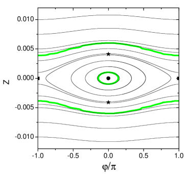
Figure 2: (Color online) Phase diagram of the improved TM model for imbalance $Z$ and phase difference $\varphi$. The circle and square points respectively indicate the positions of the minimum and saddle points of the Hamiltonian (20), while the star points correspond to the critical value $|Z_{c}|$ (23). We have also depicted as thicker (green) solid lines the results of the GP simulation for the initial conditions $(|Z|,\varphi)=(0.001,0)$ and $(|Z|,\varphi)=(0.006,0)$.

We want to note that the Bloch states of Ref. Jezek and Cataldo (2011) correspond to equally populated wells with different winding numbers. In the double-well potential these states are represented by the stationary points located at $Z=0$ in Fig. 2. The minimum at $\varphi=0$ corresponds to a vanishing winding number, while the saddle point at $|\varphi|=\pi$ corresponds to winding numbers with $|n|=1$. The latter, however, does not correspond to a vortex state, since it possesses zero angular momentum, as discussed in Ref. Jezek and Cataldo (2011).

Typical time evolutions of Josephson oscillations and ST orbits are shown in Figs. 3 and 4, respectively. In Fig. 3 we depict $Z$ and $\varphi$ as functions of time for the GP simulations (solid line), together with the results arising from the TM model (dot-dashed (blue) line). On the other hand, Fig. 4 shows the same evolutions for a larger initial imbalance, where we clearly observe a self-trapping behavior. In both cases we may see that the TM model predicts a faster dynamics than the GP simulation. As we will show in the next subsection, such a discrepancy can be substantially reduced when using a renormalized on-site interaction energy parameter (dashed (red) line).

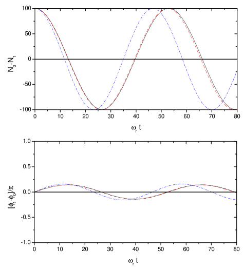
Figure 3: (Color online) Josephson oscillation in the double-well system with an initial imbalance $Z=10^{-3}$. Imbalance (top panel) and phase difference (bottom panel) are depicted as functions of time. The solid line corresponds to the GP simulation, while the dot-dashed (blue) and dashed (red) lines correspond to TM evolutions with $U=6.73\times 10^{-4}\,\hbar\omega_{r}$ and a renormalized on-site energy parameter $U_{R}=5.28\times 10^{-4}\,\hbar\omega_{r}$, respectively.

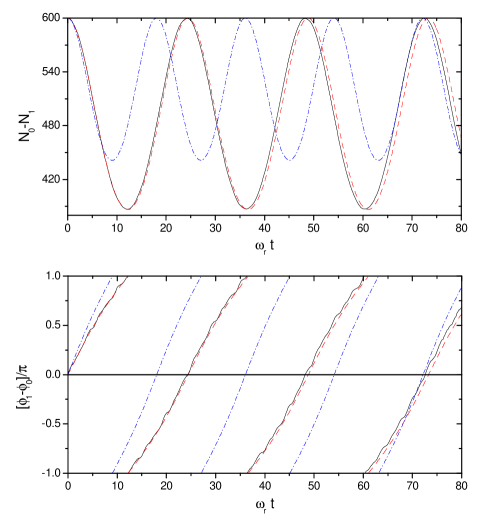
Figure 4: (Color online) Same as Fig. 3 for a self-trapping evolution with an initial imbalance $Z=6\times 10^{-3}$.

IV.3 Characteristic times

In this subsection we will derive a formula for the period of ST oscillations. Before this, we recall that the Josephson period in the limit of small oscillations reads Smerzi et al. (1997); Melé-Messeguer et al. (2011),

$$T_{\rm so}=\frac{\pi\hbar}{J_{\rm eff}\sqrt{\Lambda_{\rm eff}+1}}\,.$$ (25)

Replacing in the above equation the values of Sec. IV.2, we obtain $T_{\rm so}=46.0\,\,\,\omega_{r}^{-1}$. This is a rather good estimate of the TM period in Fig. 3 ( $T_{\rm TM}=46.68\,\,\,\omega_{r}^{-1}$), but it clearly underestimates the corresponding GP period ($T_{\rm GP}\simeq 53,09\,\,\,\omega_{r}^{-1}$).

On the other hand, the phase difference increases almost linearly with time for small imbalance oscillations in the ST regime,

$$\varphi(t)\simeq\frac{2\pi}{T_{\rm ST}}t\,,$$ (26)

as seen in Fig. 4. Now, to be consistent with this approximation, we first rewrite Eq. (19) without the adimensionalized time, and next approximate such an expression for $\Lambda_{\rm eff}=\frac{UN}{2J_{\rm eff}}>>1$ and $|Z|<<1$ as follows,

$$\frac{d\varphi}{dt}=\frac{NU}{\hbar}Z+\frac{2J_{\rm eff}}{\hbar}\left[\frac{Z}{\sqrt{1-Z^{2}}}\right]\cos\varphi\simeq\frac{NU}{\hbar}Z\simeq\frac{NU}{\hbar}Z_{0},$$ (27)

where $Z_{0}=\overline{Z(t)}$ denotes the mean value of the time dependent imbalance. Note in Fig. 4 that the maximum departure of $Z(t)$ from such a mean value lies within a $20$ percent. Therefore, from (26) and (27) we may estimate the ST period as,

$$T_{\rm ST}=\frac{2\pi\hbar}{U\overline{\Delta N}}\,,$$ (28)

where $\overline{\Delta N}=Z_{0}\,N$ denotes the time average of the particle number difference between sites. If we calculate such an average from the TM model of Fig. 4, we obtain $\overline{\Delta N}\simeq 520$, from which Eq. (28) yields $T_{\rm ST}=17.94\,\,\omega_{r}^{-1}$, that is a good estimate of the TM period of $18.04\,\,\omega_{r}^{-1}$ in Fig. 4. Now, given that the TM dynamics turns out to be noticeably faster than the GP evolution, while conserving the shape, it suggests that a renormalized value of $U$ in (28) could heal this mismatch. In fact, being $T_{\rm GP}=24.1\,\,\omega_{r}^{-1}$ and $\overline{\Delta N}_{\rm GP}=494$, we may propose to replace $U$ in Eq. (28) by the following renormalized on-site interaction energy parameter:

$$U_{R}=\frac{2\pi\hbar}{T_{\rm GP}\overline{\Delta N}_{\rm GP}}=5.28\times 10^{-4}\,\hbar\omega_{r}\,.$$ (29)

Thus, we have repeated the numerical calculations of the TM model with the above parameter, finding an excellent agreement with the GP results, as clearly observed in Figs. 3 and 4. It is also remarkable that the period for small Josephson oscillations (25), gets now closer to the GP value when using the renormalized parameter (29) ($T_{\rm so}=51.5\,\omega_{r}^{-1}$). Therefore, a more accurate Hamiltonian (20) can be constructed by replacing $U$ by $U_{R}$ in $\Lambda_{\rm eff}$.

V Multiple-mode dynamical equations

The two-mode equations describing the boson Josephson junction dynamics of two weakly coupled Bose-Einstein condensates Raghavan et al. (1999), along with their recent improvements for high particle numbers Ananikian and Bergeman (2006); Xin Yan Jia et al. (2008), can be generalized to multiple-mode (MM) dynamical equations for $N_{c}$ Bose-Einstein condensates forming a ring. In fact, we look for a solution of the time-dependent GP equation

$$i\hbar\frac{\partial\psi_{\rm MM}(r,\theta,t)}{\partial t}=\left[-\frac{\hbar^{2}}{2m}{\bf\nabla}^{2}+V_{\rm{trap}}(r,\theta)+g\,N|\psi_{\rm MM}(r,\theta,t)|^{2}\right]\psi_{\rm MM}(r,\theta,t)$$ (30)

within the variational ansatz

$$\psi_{\rm MM}(r,\theta,t)=\sum_{k=0}^{N_{c}-1}b_{k}(t)\,\,w_{k}(r,\theta),$$ (31)

where the phase of the time-dependent complex amplitude $b_{k}$ corresponds to the uniform phase of the order parameter at the $k$-th site, while $N|b_{k}|^{2}$ yields the site population. Then, replacing (31) in (30) and making use of the orthonormality of the set of WL functions, we may extract the following system of $N_{c}$ nonlinear equations,

$$i\hbar\,\frac{db_{k}}{dt} = \varepsilon b_{k}-J(b_{k-1}+b_{k+1})+UN|b_{k}|^{2}b_{k}-\frac{J^{\prime}}{2}N\{2{\rm Re}[b_{k}^{*}(b_{k-1}+b_{k+1})]b_{k}$$ (32)

$$+ (|b_{k}|^{2}+|b_{k-1}|^{2})b_{k-1}+(|b_{k}|^{2}+|b_{k+1}|^{2})b_{k+1}\}.$$

Note that the above expression assumes that each site $k$ is surrounded by two different neighbors $k-1$ and $k+1$, for that reason the $N_{c}=2$ case has been treated separately. In addition, the site denoted by $k=N_{c}$ ($k=-1$) must be identified with that of $k=0$ ($k=N_{c}-1$). If we use $b_{k}=|b_{k}|e^{i\phi_{k}}$, the time derivative in (32) reads

$$i\hbar\,\frac{db_{k}}{dt}=\hbar\,(i\frac{d|b_{k}|}{dt}-\,|b_{k}|\frac{d\phi_{k}}{dt})e^{i\phi_{k}}.$$ (33)

Next, replacing (33) in (32), multiplying this equation by $e^{-i\phi_{k}}$ and separating the real and imaginary parts, one can, after some algebra, decouple Eq. (32) into the following $2N_{c}$ real equations, written in terms of population $n_{k}=|b_{k}|^{2}=N_{k}/N$ and phase difference $\varphi_{k}=\phi_{k}-\phi_{k-1}$,

$$\hbar\,\frac{dn_{k}}{dt} = -2J[\sqrt{n_{k}\,n_{k+1}}\,\sin\varphi_{k+1}-\sqrt{n_{k}\,n_{k-1}}\,\sin\varphi_{k}]$$ (34)

$$- J^{\prime}N[\sqrt{n_{k}\,n_{k+1}}(n_{k}+n_{k+1})\,\sin\varphi_{k+1}-\sqrt{n_{k}\,n_{k-1}}(n_{k}+n_{k-1})\,\sin\varphi_{k}]$$

$$\hbar\,\frac{d\varphi_{k}}{dt} = UN(n_{k-1}-n_{k})$$ (35)

$$- J\left[\left(\sqrt{\frac{n_{k}}{n_{k-1}}}-\sqrt{\frac{n_{k-1}}{n_{k}}}\,\right)\,\cos\varphi_{k}+\sqrt{\frac{n_{k-2}}{n_{k-1}}}\,\cos\varphi_{k-1}-\sqrt{\frac{n_{k+1}}{n_{k}}}\,\cos\varphi_{k+1}\right]$$

$$- \frac{J^{\prime}N}{2}\left[\left(n_{k}\sqrt{\frac{n_{k}}{n_{k-1}}}-n_{k-1}\sqrt{\frac{n_{k-1}}{n_{k}}}\,\right)\,\cos\varphi_{k}+\left(3\,\sqrt{n_{k-2}\,n_{k-1}}+n_{k-2}\sqrt{\frac{n_{k-2}}{n_{k-1}}}\,\right)\,\cos\varphi_{k-1}\right.$$

$$- \left.\left(3\,\sqrt{n_{k+1}\,n_{k}}+n_{k+1}\sqrt{\frac{n_{k+1}}{n_{k}}}\,\right)\,\cos\varphi_{k+1}\right].$$

The above MM dynamical equations constitute the generalization of the TM pair of equations (18) and (19) for $N_{c}>2$. Note that similarly to the TM case, only $2N_{c}-2$ of the above equations are independent since the variables must fulfill $\sum_{k}n_{k}=1$ and $\sum_{k}\varphi_{k}=0$.

V.1 Four-well ring lattice

In order to compare the MM dynamics with the results of GP simulations, we have numerically integrated the system (34)-(35) for $N_{c}=4$ and two initial configurations. The model parameters utilized in this case were $U=1.38\times 10^{-3}\,\hbar\omega_{r}$, $J=-4.98\times 10^{-4}\,\hbar\omega_{r}$ and $J^{\prime}=2.76\times 10^{-8}\,\hbar\omega_{r}$.

V.1.1 Symmetric case

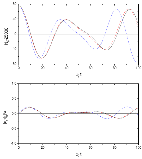
Figure 5: (Color online) Time evolution of population $N_{0}-M$ (top panel) and phase difference $\phi_{1}-\phi_{0}$ (bottom panel), for the four-well system and an initial condition $N_{0}-M=75$, $N_{k}-M=-25$ ($k=1,2,3$) with an uniformly vanishing phase. The solid line corresponds to the GP simulation, while the dot-dashed (blue) and dashed (red) lines correspond to the MM and RMM models, with on-site interaction energy parameters $U=1.38\times 10^{-3}\,\hbar\omega_{r}$ and $U_{R}=1.08\times 10^{-3}\,\hbar\omega_{r}$, respectively.

Here we consider initial conditions which are symmetric with respect to the right and left from the $k=0$ well, as also studied by De Liberato and Foot in Ref. S. De Liberato and Foot (2006). Particularly, in Fig. 5 we have chosen the following initial condition: $N_{0}-M=75$ and $N_{k}-M=-25$ for the remaining sites, where $M=N/N_{c}=25000$ denotes the mean number of particles per site in the ground state. We may observe in the top panel that the population oscillates around the mean value $M$ without any periodicity, at least for the times involved in our numerical simulations. A similar behavior for the phase difference has been depicted in the bottom panel of Fig. 5. Note that the MM model again reproduces the shape of the GP evolution in a faster dynamics, as already observed for the TM model.

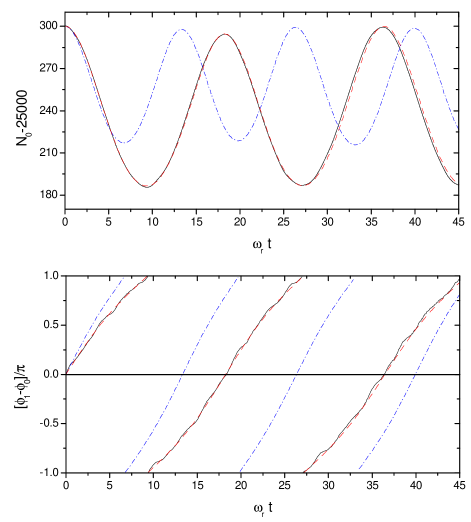
Figure 6: (Color online) Same as Fig. 5 for an initial condition $N_{0}-M=300$ and $N_{k}-M=-100$ ($k=1,2,3$).

Figure 6 shows the time evolution for the same symmetric initial configuration, but with a higher population in the $k=0$ well ($N_{0}-M=300$, $N_{k}-M=-100$ for $k=1,2,3$). We observe in this case a clear ST regime, with the population $N_{0}-M$, which keeps positive during the oscillations performed around $N_{0}-25000\simeq 240$, and an unbounded phase that increases almost linearly with time.

Now we will generalize the treatment of Sec. IV.3, to estimate the ST period in order to derive a renormalized on-site energy parameter. First, according to the bottom panel of Fig. 6 we may approximate (cf Eq. (26))

$$\varphi_{1}(t)\simeq\frac{2\pi}{T_{\rm ST}}t,$$ (36)

and next, consistent with this approximation (cf Eq. (27)), we approximate Eq. (35) as,

$$\frac{d\varphi_{1}}{dt}\simeq\frac{UN(n_{0}-n_{1})}{\hbar}\simeq\frac{U(\overline{N_{0}-N_{1}})}{\hbar},$$ (37)

where the upper bar again denotes time average. Therefore, from (36) and (37) we may estimate the ST period as,

$$T_{\rm ST}\simeq\frac{2\pi\hbar}{U(\overline{N_{0}-N_{1}})}$$ (38)

which, taking into account the value $(\overline{N_{0}-N_{1}})=345$ extracted from the MM results, yields $T_{\rm ST}\simeq 13\,\,\omega_{r}^{-1}$, in accordance with the period of the MM model in Fig. 6 (dot-dashed (blue) lines). Then, we may repeat the procedure of Sec. IV.3 and extract a renormalized on-site interaction energy parameter,

$$U_{R}=\frac{2\pi\hbar}{T_{\rm GP}(\overline{N_{0}-N_{1}})_{\rm GP}}\,,$$ (39)

where the values $(\overline{N_{0}-N_{1}})_{\rm GP}=323$ and $T_{\rm GP}\simeq 18\,\,\omega_{r}^{-1}$, arising from the GP simulation results, yield $U_{R}=1.08\times 10^{-3}\,\hbar\omega_{r}$. The use of this renormalized $U$ parameter in the MM calculations leads to a much better agreement with the GP results, as clearly shown in Figs. 5 and 6. We will call this improved MM model as the renormalized multiple-mode (RMM) model.

V.1.2 Non symmetric case

To test the quality of the above RMM model, we will analyze the time evolution of two non symmetric initial configurations utilizing the same value for $U_{R}$ extracted in the previous section. In Figs. 7 and 8, we have plotted the population and phase differences between adjacent sites, respectively, for an initial condition $N_{0}-M=600$, $N_{1}-M=-300$, $N_{2}-M=-200$, and $N_{3}-M=-100$. We may observe that the RMM model fits much more accurately the GP simulation results than the original MM model. A similar improvement may be observed in Figs. 9 and 10 for the second initial condition, $N_{0}-M=300$, $N_{1}-M=-300$, and $N_{k}-M=0$ for $k=2,3$. As inferred from Figs. 7 and 8, such a configuration presents self-trapping in the $k=0$ site, while for the second initial condition, this system exhibits self-trapping in the $k=0$ site, self-depletion in the $k=1$ site, and an irregular oscillatory dynamics around the mean number of particles on the remaining wells, as seen from Figs. 9 and 10. The latter configuration had been previously described by means of a standard MM model by De Liberato and Foot S. De Liberato and Foot (2006).

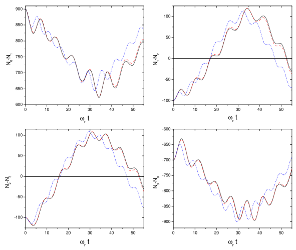
Figure 7: (Color online) Particle number differences between neighboring sites for $N_{c}=4$ and the initial condition $N_{0}-M=600$, $N_{1}-M=-300$, $N_{2}-M=-200$, and $N_{3}-M=-100$. The solid line corresponds to the GP simulation, while the dot-dashed (blue) and dashed (red) lines correspond to the MM and RMM models, with on-site interaction energy parameters $U=1.38\times 10^{-3}\,\hbar\omega_{r}$ and $U_{R}=1.08\times 10^{-3}\,\hbar\omega_{r}$, respectively.

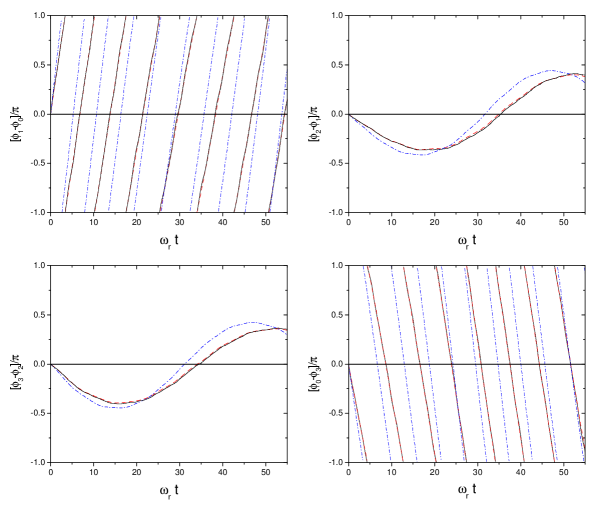
Figure 8: (Color online) Same as Fig. 7 for the phase differences between neighboring sites.

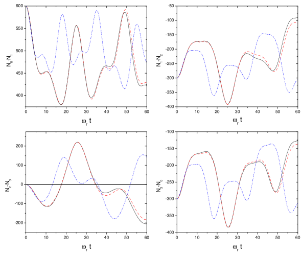
Figure 9: (Color online) Same as Fig. 7 for an initial condition $N_{0}-M=300$, $N_{1}-M=-300$, $N_{k}-M=0$ ($k=2,3$).

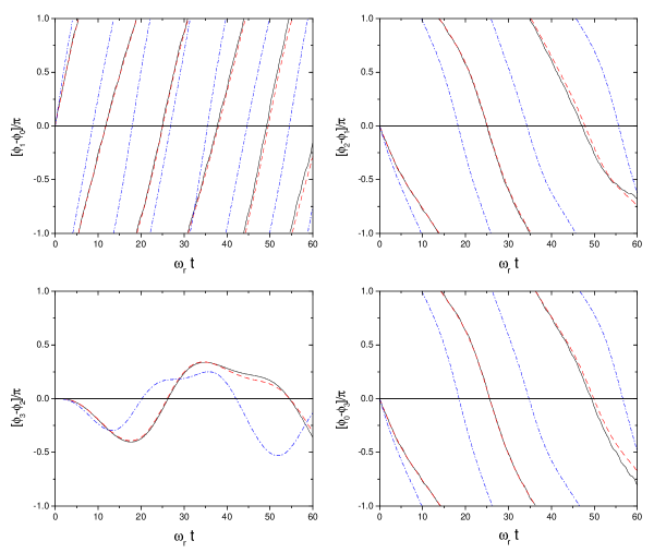
Figure 10: (Color online) Same as Fig. 9 for the phase differences between neighboring sites.

V.2 Eight-well ring lattice

To conclude we will explore a ring lattice consisting of a larger number of wells, $N_{c}=8$. The corresponding MM parameters are as follows, $U=2.918\times 10^{-3}\,\hbar\omega_{r}$, $J=-1.898\times 10^{-3}\,\hbar\omega_{r}$, and $J^{\prime}=2.118\times 10^{-7}\,\hbar\omega_{r}$. In Fig. 11, we have depicted the population of the site $k=0$ and the phase difference between the $k=1$ and $k=0$ sites, for three different initial conditions.

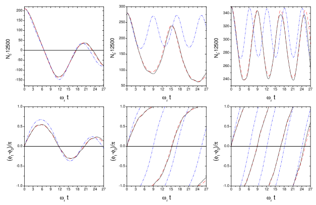
Figure 11: (Color online) Population of the $k=0$ well (upper panels) and phase difference between the $k=1$ and $k=0$ wells (lower panels) for $N_{c}=8$ and the initial conditions: $N_{0}-M=210$, $N_{k}-M=-30$ ($1\leq k\leq 7$) (left panels); $N_{0}-M=280$, $N_{k}-M=-40$ ($1\leq k\leq 7$) (central panels) and $N_{0}-M=350$, $N_{k}-M=-50$ ($1\leq k\leq 7$) (right panels). The solid line corresponds to the GP simulation, while the dot-dashed (blue) and dashed (red) lines correspond to the MM and RMM models, with on-site interaction energy parameters $U=2.918\times 10^{-3}\,\hbar\omega_{r}$ and $U_{R}=2.2\times 10^{-3}\,\hbar\omega_{r}$, respectively.

Then, we may obtain as before a renormalized on-site energy parameter $U_{R}$ from the GP results of the ST regime depicted on the right panels of Fig. 11. In fact, replacing the ST period $T_{\rm GP}\simeq 8.4\,\,\omega_{r}^{-1}$ and the average difference $(\overline{N_{0}-N_{1}})_{\rm GP}\simeq 335$ in Eq. (39), we obtain a RMM model parameter $U_{R}=2.2\times 10^{-3}$, which yields a sizable improvement to the MM results, as seen in Fig. 11.

VI Calculation of the effective interaction energy parameter using the ground-state density

Recently it has been demonstrated Jezek et al. (2013); *cond that for a double-well system, the on-site interaction energy dependence on the imbalance should be taken into account in the two-mode model, in order to accurately describe the exact dynamics. There, using a Thomas-Fermi density, a linear dependence with the imbalance has been analytically encountered, and this has been shown to give rise to an effective interaction energy parameter in the two-mode equations of motion. Here we generalize, beyond the Thomas-Fermi approximation, that result to the case of multiple-well configurations. Following the procedure of Ref. Jezek et al. (2013); *cond adapted to $N_{c}$ wells and using numerically obtained densities, we have to evaluate the quotient

$$\frac{U_{k}}{U}\simeq\frac{\int d^{2}{\bf r}\,\,\rho_{N}({\bf r})\,\rho_{N+\Delta N}({\bf r})}{\int d^{2}{\bf r}\,\,\rho^{2}_{N}({\bf r})},$$ (40)

where we have further assumed in (40) that instead of localized on-site densities, we may use the ground-state densities $\rho_{N}({\bf r})$ and $\rho_{N+\Delta N}({\bf r})$ normalized to unity of systems with $N$ and $N+\Delta N$ particles, respectively, being $\Delta N=N_{c}\Delta N_{k}=N_{c}N_{k}-N$.

Numerical calculations of the r.h.s. of (40) are depicted in Fig. 12, where we may observe a linear behavior with $N_{c}\Delta N_{k}/N$ for different numbers of lattice sites.

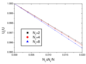
Figure 12: (Color online) Numerical calculation of the right-hand side of Eq. (40) versus $N_{c}\Delta N_{k}/N$ for three numbers of lattice sites. The (black) squares, (red) circles, and (blue) triangles correspond to $N_{c}=2$, 4, and 8, respectively, while each line corresponds to a linear fit.

Note that the apparent counterintuitive decrease of this function with the site population is related to the fact that the densities must be normalized to unity.

Taking into account this linear dependence of the on-site energy parameter we may write

$$\frac{U_{k}}{U}\simeq 1-\alpha\frac{N_{c}\Delta N_{k}}{N},$$ (41)

where the values of $\alpha$ in Table 1 correspond to the linear fits of the points in Fig. 12. To include this correction in the MM model we must evaluate Jezek et al. (2013); *cond,

$$\frac{U_{k-1}}{U}N_{k-1}-\frac{U_{k}}{U}N_{k}=\left(1-\alpha\frac{N_{c}\Delta N_{k-1}}{N}\right)\left(\Delta N_{k-1}+\frac{N}{N_{c}}\right)-\left(1-\alpha\frac{N_{c}\Delta N_{k}}{N}\right)\left(\Delta N_{k}+\frac{N}{N_{c}}\right)$$ (42)

which yields,

$$\frac{U_{k-1}}{U}N_{k-1}-\frac{U_{k}}{U}N_{k}=(1-\alpha)(N_{k-1}-N_{k})-\alpha(N_{k-1}-N_{k})[\frac{N_{c}(N_{k-1}+N_{k})}{N}-2].$$ (43)

And finally replace the last result in the first term of the r.h.s. of Eqs. (19) and (35). By analyzing the term

$$\alpha(N_{k-1}-N_{k})[\frac{N_{c}(N_{k-1}+N_{k})}{N}-2]=\alpha(N_{k-1}-N_{k})\frac{N_{c}(\Delta N_{k-1}+\Delta N_{k})}{N},$$ (44)

we first note that in the double well case it is identically zero, while for other studied cases $\frac{N_{c}(\Delta N_{k-1}+\Delta N_{k})}{N}<<1$ (cf. the range of $N_{c}\Delta N_{k}/N$ in Fig. 12). Thus, disregarding such a term, we in fact obtain a correction that can be regarded as a reduced effective interaction parameter $\tilde{U}=(1-\alpha)U$. Note that this result is in accordance with our previous analysis which yielded the renormalized parameter $U_{R}$ using characteristic times, while the corresponding quantitative agreement is shown in Table 1.

Table 1: Linear correction coefficient $\alpha$ of the on-site interaction energy parameter of the $k$-site (Eq. (41)), and effective $\tilde{U}$, renormalized $U_{R}$, and bare $U$ interaction energy parameters, for three numbers of wells $N_{c}$. The interaction energy parameters are given in units of $\hbar\omega_{r}$.

$N_{c}$	$\alpha$	$\tilde{U}$	$U_{R}$	$U$
2	$0.208$	$5.33\times 10^{-4}$	$5.28\times 10^{-4}$	$6.73\times 10^{-4}$
4	$0.214$	$1.09\times 10^{-3}$	$1.08\times 10^{-3}$	$1.38\times 10^{-3}$
8	$0.228$	$2.25\times 10^{-3}$	$2.22\times 10^{-3}$	$2.92\times 10^{-3}$

VII Summary and concluding remarks

We have investigated the dynamics of ring-shaped optical lattices with a high number of particles per site. To this aim, we have derived the equations of motion for population and phase differences between neighboring sites of a generalized multimode model that utilizes a localized on-site Wannier-like basis. We have shown that in case of a double-well system, this approach coincides with the latest improved two-mode model Ananikian and Bergeman (2006).

To test the quality of our model, we have numerically solved the time dependent GP equation for different numbers of wells, particularly $2$, $4$, and $8$. By realizing that the self-trapping time period turns out to be chiefly ruled by the on-site interaction energy parameter, and utilizing the output of a single GP simulation, we were able to renormalize such a parameter. The use of this renormalized parameter in the multimode equations strikingly led to a much better agreement with the GP results for all investigated initial conditions, of which only a few representative were included in this report. Finally, we have shown that the effective interaction energy parameter, which takes into account the deformation of the density during the time evolution, yields results that are in good agreement with the previously obtained for the renormalized parameter.

To conclude, we wish to emphasize that the two-mode model has predicted, even in its improved version Ananikian and Bergeman (2006), a sizable faster evolution than our GP simulation results, as discussed in Sec. IV.3. The same behavior is observed in previous experimental and theoretical works dealing with other type of double-well systems (see, e.g., Melé-Messeguer et al. (2011); Gati and Oberthaler (2007) and references therein). We believe that also in these systems as in our case, the TM model with an effective reduction of the on-site interaction energy parameter numerically calculated as here proposed, should provide a more accurate dynamics.