Production of minimally entangled typical thermal states
with the Krylov-space approach

Abstract

The minimally entangled typical thermal states algorithm is applied to fermionic systems using the Krylov-space approach to evolve the system in imaginary time. The convergence of local observables is studied in a tight-binding system with a site-dependent potential. The temperature dependence of the superconducting correlations of the attractive Hubbard model is analyzed on chains, showing an exponential decay with distance and exponents proportional to the temperature at low temperatures, as expected. In addition, the non-local parity correlator is calculated at finite temperature. Other possible applications of the minimally entangled typical thermal states algorithm to fermionic systems are also discussed.

I Introduction

Originally, the density matrix renormalization groupWhite (1992, 1993) (DMRG) algorithm dealt with zero temperature or ground-state properties. The development of the algorithm at finite temperature has been a topic of much interest,Verstraete et al. (2004); Zwolak and Vidal (2004); Feiguin and White (2005) because of the increased complexity associated with efficiently computing temperature-dependent properties.

Recently, White(White, 2009) proposed an efficient method—that he refers to as minimally entangled typical thermal states or METTS—to compute temperature-dependent observables with a complexity similar to ground state computations. An observable $\hat{A}$ of a quantum many body system at temperature $T=1/(k_{B}\beta)$ is expressed as $\langle A\rangle={\rm Tr}{[}\hat{\rho}\hat{A}{]}=1/\mathcal{Z}{\rm Tr}{[}{\rm e}^{-\beta\hat{H}}\hat{A}{]}$, the trace involving two kinds of integration: over quantum and thermal fluctuations. Performing this calculation directly is intractable, even more so than at zero temperature. One can, however, approximate the expectation value of $A$ by strategies based on sampling. The METTS algorithmWhite (2009) starts from classical product states, and then entanglement is brought about by the (imaginary) time evolution of those initial states.

In METTS, thermal fluctuations are sampled by randomly selecting quantum states. To understand how this is done let us first expand the trace in terms of an orthonormal basis $|i\rangle$, such that $\langle A\rangle=\frac{1}{\mathcal{Z}}\sum_{i}P(i)\langle\phi(i)|A|\phi(i)\rangle,$ where $|\phi(i)\rangle=P(i)^{-1/2}{\rm e}^{-\beta H/2}|i\rangle$ and $P(i)=\langle i|e^{-\beta H/2}|i\rangle$. A choice for the basis $|i\rangle$ is the set of classical product states (CPS); these are states with wavefunctions $|i\rangle=|i_{0}\rangle|i_{1}\rangle\cdots|i_{N-1}\rangle$, where the labels 0, 1, 2, …, refer to the sites of the lattice. The essence of the method lies in the way $\langle A\rangle$ is estimated by sampling the states $|\phi(i)\rangle$ with probability $P(i)/\mathcal{Z}$, and by averaging the expectation values $\langle\phi(i)|A|\phi(i)\rangle$ computed at each step. A proof that the ensemble $\{|\phi(i)\rangle\}$ so generated correctly reproduces all thermodynamic measurements is given in reference White, 2009, as well as a justification for referring to the set $\{|\phi(i)\rangle\}$ as METTS. In addition to the original reference,White (2009) a matrix-product-state formulation of the method can be found in references Stoudenmire and White, 2010; Schollwöck, 2010, as well as a viewpoint in Physics.(Schollwöck, 2009)

Quantum Monte Carlo methods can also simulate strongly correlated electron models at finite temperature. The use of finite-temperature DMRG has, however, advantages and disadvantages that make it an ideal complementary method. Finite-temperature DMRG is advantageous in the case of long chains, and even ladder geometries. Moreover, for those strongly correlated electron models where the sign problem hinders quantum Monte Carlo simulations, DMRG methods can come to the rescue. They might be the only unbiased technique applicable to models with, for example, spin flipping terms, which are known to present serious sign problems. This is exactly the case of iron-Kamihara et al. (2008) and selenide-basedGuo et al. (2005) superconductors, which include J termsDaghofer et al. (2008); Moreo et al. (2008) (as in the case of t-J models). Thus, the METTS algorithm might be particularly appropriate for these superconductors.

This paper explains in detail the production and use of METTS with the Krylov-space approach for DMRG time evolutionManmana et al. (2005); Schollwöeck and White (2006); Schollwöck (2005). Section II describes the implementation of the algorithm, including the “collapse” procedure, the ergodicity issues, and the computational complexity. Section III focuses on local observables in the case of a fermionic non-interacting system with a site-dependent potential. The attractive Hubbard model at quarter filling is then studied for a one-dimensional open geometry (chain), and superconducting correlations are compared to known results. The non-local parity correlator is then calculated at finite temperature. Finally, section IV presents an outlook for the further applicability of METTS.

II Algorithm

II.1 Production of METTS

Here the Krylov-space approach for time evolution is adapted to produce minimally entangled typical thermal states or METTS,White (2009); Stoudenmire and White (2010) that is, a “thermal” evolution is produced. The natural real-space basis of a model is defined as the set of states in its one-site Hilbert space. For example, the natural basis is composed of the states empty, up, down, and doubly occupied in the case of the one-orbital Hubbard model. The notation $\mathcal{N}{|x\rangle\equiv|x\rangle/|||x\rangle||}$ appears below to simplify the expressions.

The steps to obtain observables at any target inverse temperature $\beta_{\rm T}$ are as follows.

(1) Set the current inverse temperature $\beta_{\rm C}=0$. Do a standard “infinite DMRG,” and grow the $N-$site lattice, choosing a random real-space basis state per site to create a pure state. Target this pure state at each step, that is, include it in the reduced density matrix. Proceed in this way until all sites have been added and end up with a pure state over the whole lattice: $|\pi\rangle=|i_{0}\rangle|i_{1}\rangle...|i_{N-1}\rangle$.

(2) Obtain the states $|\phi(k)\rangle=\mathcal{N}{\exp(-\beta_{k}H/2)|\pi\rangle}$, $0\leq k<l$, using a Krylov-space approach for the time evolution;Manmana et al. (2005); Schollwöeck and White (2006); Schollwöck (2005) an implementation can be found in reference Alvarez et al., 2011. Here $\beta_{k}=k\tau/(l-1)$, $\tau=0.1$, $l=5$. Collapse (the collapse is described in section II.2) the last one, $|\phi(l-1)\rangle$, into a pure state $|\pi^{\prime}\rangle$. Target $|\phi(k)\rangle$ $0\leq k<l$, and $|\pi^{\prime}\rangle$.

(3) Move the center of orthogonality by one, as “finite” DMRG does. Wave-function transform $|\phi(k=0)\rangle$ (also denoted by $|\pi\rangle$) into ${\rm Wft}(|\phi(k=0)\rangle)$. Recompute $\exp(-\beta_{k}H/2){\rm Wft}(|\phi(k)\rangle)$ $\forall\,1\leq k<l$. Wave-function transform also the collapsed state $|\pi^{\prime}\rangle$. Proceed sweeping the lattice for a while, until, for example, an extreme is reached, or all sites have been visited at least once.

(4) If $\beta_{\rm C}<\beta_{\rm T}$ then advance in $\beta$: Set $|\phi(k=0)\rangle\equiv|\pi\rangle$ to $|\phi(k=l-1)\rangle$. Increase $\beta_{\rm C}$ by $\tau$. Go to step (2). If $\beta_{\rm C}=\beta_{\rm T}$ then perform a measurement (for production runs, instead of measuring in situ, save the METTS to measure post-processing) using the current wave-function transformed $|\phi(k=0)\rangle$. Set the state $|\phi(k=0)\rangle$ to the wave-function transformed collapsed $|\pi^{\prime}\rangle$. In other words, set $|\pi\rangle$ to $|\pi^{\prime}\rangle$. Set $\beta_{\rm C}=0$ and go to step (2).

II.2 Collapsing METTS

Let us consider first the collapse into the natural basis and then into a random basis.

If the collapse happens in the real-space basis then for a Hubbard model with only one orbital there are four states to collapse into: empty, up, down, and doubly occupied. If $|\phi(k)\rangle$ (or its wave-function transformed form) is centered on site $i$ then $|\phi(k)\rangle=\sum_{\alpha_{L},\alpha_{i},\alpha_{R}}A_{\alpha_{L},\alpha_{i},\alpha_{R}}|\alpha_{L}\rangle|\alpha_{i}\rangle|\alpha_{R}\rangle$, where $\alpha_{i}$ is a state of the natural real-space basis. This state is normalized, hence $\sum_{\alpha_{L},\alpha_{i},\alpha_{R}}|A_{\alpha_{L},\alpha_{i},\alpha_{R}}|^{2}=1$.

Let $|\pi(\alpha_{i})\rangle=\sum_{\alpha_{L},\alpha_{R}}A_{\alpha_{L},\alpha_{i},\alpha_{R}}|\alpha_{L}\rangle|\alpha_{i}\rangle|\alpha_{R}\rangle$, for each state $\alpha_{i}$ of the natural one-site basis at $i$. Let $p(\alpha_{i})=||\pi(\alpha_{i})\rangle||^{2}$. The condition $\sum_{\alpha_{i}}p(\alpha_{i})=1$ follows from the normalization of $|\phi(k)\rangle$. A state $\alpha_{i}$ is selected with probability $p(\alpha_{i})$ and the collapse occurs into the state $|\pi^{\prime}\rangle=\mathcal{N}|\pi(\alpha_{i})\rangle$, which is now to be used for step (2).

When the collapse happens in a random basis defined by $|\alpha_{i}\rangle=\sum_{\eta_{i}}M_{\alpha_{i},\eta_{i}}|\eta_{i}\rangle$ we proceed as follows. First we rewrite

$$|\phi(k)\rangle=\sum_{\alpha_{L},\alpha_{i},\alpha_{R}}A_{\alpha_{L},\alpha_{i},\alpha_{R}}\sum_{\eta_{i}}M_{\alpha_{i},\eta_{i}}|\alpha_{L}\rangle|\eta_{i}\rangle|\alpha_{R}\rangle.$$ (1)

Defining $|\bar{\pi}(\eta_{i})\rangle$ by $|\phi(k)\rangle=\sum_{\eta_{i}}|\bar{\pi}(\eta_{i})\rangle$, for each state $\eta_{i}$ of the random basis, yields

$$|\bar{\pi}(\eta_{i})\rangle=\sum_{\alpha_{L},\alpha_{i},\alpha^{\prime}_{i},\alpha_{R}}M^{-1}_{\eta_{i},\alpha^{\prime}_{i}}A_{\alpha_{L},\alpha_{i},\alpha_{R}}M_{\alpha_{i},\eta_{i}}|\alpha_{L}\rangle|\alpha^{\prime}_{i}\rangle|\alpha_{R}\rangle.$$ (2)

The new state $\mathcal{N}\bar{\pi}(\eta_{i})$ is collapsed with probability $p(\eta_{i})=||\bar{\pi}(\eta_{i})\rangle||^{2}$; these probabilities add up to 1 because of normalization.

One important practical consequence of these collapse equations is that they do not preserve local symmetries unless the collapse basis does, implying that simulations, in most cases, will have to be performed in the grand canonical ensemble. Indeed, all METTS simulations in this paper are done in the grand canonical ensemble, as we will see in the next sections.

II.3 Ergodicity

To illustrate ergodicity issues with this technique let us consider a tight-binding chain and a chemical potential term such that $H=\sum_{i,j}t_{ij}c^{\dagger}_{i}c_{j}+\mu\sum_{i}n_{i}$, where $t_{ij}=1$ if $i$ and $j$ are nearest neighbors and $0$ otherwise. As observables let us consider the total energy and density of the system at inverse temperature $\beta$. These observables depend on $\mu$, but if we use the natural basis for the collapse, the method will (incorrectly) yield values independent of $\mu$. To understand the reason for the second statement I would now like to show that, if we collapse only to the natural basis, METTS do not depend on $\mu$. Let us choose an initial CPS $|\pi\rangle$, and compute the corresponding METTS at $\beta$. Note that $|\pi\rangle$ is an eigenvector of $\mu\sum_{i}n_{i}$. The resulting METTS is $\exp(-\beta H_{0})|\pi\rangle/\langle\pi|\exp(-\beta H_{0})|\pi\rangle$, where $H_{0}=\sum_{i,j}t_{ij}c^{\dagger}_{i}c_{j}$ does not contain $\mu$, which canceled out due to normalization. If we now proceed to collapse this METTS into a CPS in the natural basis, we obtain the CPS $|\pi^{\prime}\rangle$. Evolving $|\pi^{\prime}\rangle$ does not involve $\mu$, as $|\pi^{\prime}\rangle$ is an eigenvector of $\mu\sum_{i}n_{i}$. Therefore, all the METTS thus obtained are independent of $\mu$ and, when measuring over them, we will (incorrectly) obtain values independent of $\mu$.

In this case the solution is simple: the collapse must be carried out into a random basis and not into the natural basis. Results are shown in figure 1. In general, the Hamiltonian can be decomposed as $H=\sum_{x}H_{x}$ where each term $H_{x}$ is either a connection $\sum_{i,j}t^{x}_{ij}A^{x}_{i}B^{x}_{j}$ or an on-site term $\sum_{i}C^{x}_{i}$. (This decomposition is unique up to a canonical transformation, which would change accordingly the collapse basis, and thus, the decomposition can be considered unique for our purposes.) Therefore, a condition necessary for ergodicity is that no Hamiltonian term be diagonal in the collapse basis.

Collapse bases can but do not have to be completely random: Bases that do not mix states with different particle number or bases with the spins quantized in a given direction are examples. It has also been suggestedStoudenmire and White (2010) that changing the collapse basis from iteration to iteration (instead of keeping it fixed as has been assumed so far) improves ergodicity.

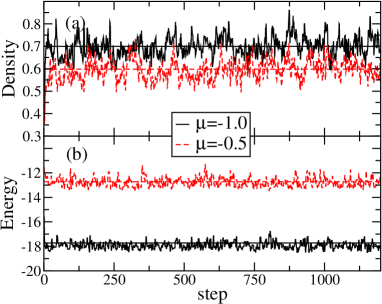
Figure 1: (Color online) (a) Density and (b) energy of electrons in a tight-binding chain with a chemical potential versus the step of the METTS algorithm. Here METTS are collapsed in a random basis, reducing ergodicity issues, and causing the observables’ average to tend to their exact values (horizontal lines).

II.4 Computational Complexity

The computational complexity of the Krylov-space approach for the time evolution was mentioned in reference Alvarez et al., 2011: The error dependence of the Krylov-space approach isManmana et al. (2005) proportional to $\exp(-(\rho dt)^{2}/(16n))(e\rho dt/(4n))^{n}$ with $n\geq\rho dt/2$ and $\rho$ the width of the spectrum, whereas in the Suzuki-Trotter approach the error is given by the Trotter error.Schollwöeck and White (2006) The Krylov-space method is independent of the form of the Hamiltonian; the Suzuki-Trotter depends on the Hamiltonian connections. The main disadvantage of the Krylov-space method is that it can be computationally more expensive compared to the Suzuki-Trotter due to the former requiring a tridiagonal decomposition of the Hamiltonian. For the production of METTS, however, there is no ground state computation, and there is a single tridiagonal decomposition needed per step. As noted in reference White, 2009, the computational complexity of the METTS algorithm is that of ground state DMRG multiplied by $\beta$ and by the number of measurements needed.

Parallelization was implemented in various places: in the Hamiltonian construction, in the construction of the density matrix, in the wave function transformations, in the computation of two-point correlations. Parallelization helps decrease the pre-factors in the CPU times, but does not affect the scaling in other ways. The CPU time required for long chains was about 12 hours for 100 METTS. These CPU times double if two-point correlations are needed. Also, sometimes multiple series of METTS need to be produced, as will be explained in the next section.

III Results

III.1 Site-dependent potential

Consider a one-orbital Hubbard model,

$$H=\sum_{i,j,\sigma}t_{ij}c^{\dagger}_{i\sigma}c_{j\sigma}+U\sum_{i}n_{i\uparrow}n_{i\downarrow}+\sum_{i,\sigma}V_{i}n_{i,\sigma},$$ (3)

where $t_{ij}$ corresponds to an open chain. First let us set $U=0$ to be able to compare with the exact result. For $N=8$ and a fixed potential profile, the energy and density were obtained by averaging over METTS. Numerical values and statistics are shown in table 1 as a function of the inverse temperature $\beta$. Higher temperatures yield larger standard deviations, but the differences with the exact results never exceed 8% for the density, and 3% for the energy. Longer runs can be performed to decrease these differences even further if necessary.

Figure 2(a) shows the resulting density profile, where only one spin sector is considered. The observable $n_{i}$ differs from the exact result more than global observables like the total energy. As mentioned, to decrease this difference longer runs could be performed, but it turns out to be better to produce multiple series of METTS started from different CPSs, and average them. The latter strategy has the advantage of completely smearing the dependence on the initial configuration, decreasing autocorrelation times faster. Figure 2(b) shows the density profile after averaging five series of METTS. On the right, the inset of figure 2 shows the maximum difference between the METTS result and the exact result at the highest temperature considered ($\beta=1.0$) as a function of the number of series of METTS used, confirming the effectiveness of this method even for a small number of series.

$\beta$	$\langle n\rangle$	Std. Dev.	Exact	$\langle E\rangle$	Std. Dev.	Exact
1.0	3.900	0.550	4.007	-7.1360	0.9715	-6.9774
2.0	4.278	0.362	4.027	-9.0594	0.5785	-9.3178
4.4	3.962	0.123	4.002	-10.4584	0.2169	-10.3515

Table 1: Mean values, standard deviations and exact results for both energy and density as a function of the inverse temperature $\beta$ for an eight-site open chain with $U=0$ and the potential profile shown in the inset of figure 2(a). Approximately 150 METTS were used.

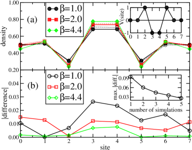
Figure 2: (Color online) (a) Density at each site of the same system as in table 1, with $\beta$ as indicated. Exact results are given by solid lines and filled symbols, METTS results by dashed lines and open symbols. Inset: potential profile for this system. (b) Unsigned difference between the density computed by the METTS algorithm and the exact one, at each site of the chain. Temperatures as before. An average over 5 series of METTS was performed. Inset: Maximum difference at $\beta=1.0$ as a function of the number of simulations, that is, the number of series of METTS used.

III.2 Attractive Hubbard Model

III.2.1 Pairing correlation

Let us now study Eq. (3) at quarter filling with $U<0$ and $V_{i}=\mu$ $\forall i$. The density ($\langle n\rangle=0.25$) is fixed on average only, and simulations are carried out in the grand canonical ensemble in order to collapse to completely random bases. A particle- (but not $S_{z}$-) conserving basis would be better here were it not for the ergodicity problems—which I have found to be too severe. The choice of model, the attractive Hubbard model, is based on the following considerations. The METTS algorithm has not been tested on fermionic systems before. The Hubbard model on a periodic chain has been solved exactly,Lieb and Wu (1968) albeit correlations are difficult to compute. The attractive Hubbard model superconducting correlations are known, and can be computed and extrapolated at moderate lattice sizes.

The s-wave pairing function (see, for example, reference Guerrero et al., 2000) $P_{s}(R)=\frac{1}{N}\sum_{i}\langle\Delta^{\dagger}_{s}(i+R)\Delta_{s}(i)\rangle$ measures superconducting correlations in this model; here $\Delta_{s}(i)=c_{i\downarrow}c_{i\uparrow}$. We are going to consider $P_{s}(R)$ as a function of temperature $T$ at quarter filling.

For $T=0$ and a periodic system $P_{s}(R)$ is knownKawakami and Yang (1991) to decay as a power law.

Studying this decay requires taking into account pairs of sites at distances as large as possible, while at the same time minimizing effects due to border sites. One possibility is to avoid some sites next to the left and right borders of the chain, and average over all other pairs at a given distance. Another possibility is to take into account all pairs of sites at distance $R$ but restrict $R$ to half the length of the chain, an approach that includes as many lattice sites as possible and avoids both sites in the pair being close to the borders for large distances. I have estimated and compared exponents of power laws following both approaches, and found small differences but no change in the trends of the exponents. Therefore, consistent with the second approach mentioned, distances $R>N/2$ were discarded in order to avoid boundary effects.

Results are shown in figure 3(a), and exponents $\bar{\beta}$ for the expression $P_{s}(R)\propto R^{-\bar{\beta}}$ in columns 2 to 4 of table 2, exponents that turn out to be comparable to those of Figure 8 of reference Kawakami and Yang, 1991 at quarter filling. (Although the standard notation for this exponent is $\beta$, the exponent is here denoted by $\bar{\beta}$ to avoid confusion with the inverse temperature.) Trying to fit these $T=0$ results to an exponential always gives larger errors than trying to fit them to a power law. For $T=0$ the power law exponents computed here with DMRG decrease with increasing $U$, as is the case in the exact thermodynamic limit results. A value of $m=200$ was used in this ground state DMRG calculation, where each site of the lattice was swept three times.

For $T>0$ $P_{s}(R)$ is knownKoma and Tasaki (1992); Tasaki (1998) to decay with exponential bounds.

Using the METTS algorithm to simulate finite temperature, a faster decay can be seen than that at $T=0$: Results for $T>0$ in figure 3(b) for $U=-2$ and figure 3(c) for $U=-4$ depart from the power law scaling (represented by a straight line in logarithmic scale), and approximate an exponential scaling $P_{s}(R)\propto\exp(-\gamma R)$. Exponents $\gamma$ for different values of $U$ are given in columns 5 to 7 of table 2. For large $\beta$, $\gamma$ must be proportional to $1/\beta$,Koma and Tasaki (1992); Tasaki (1998) and for $\beta\geq 4.4$ this relation indeed holds with 3% accuracy to 12% accuracy depending on $U$, as shown in the last column of table 2. Trying to fit METTS results (at $T>0$) to an exponential always gives smaller errors than trying to fit them to a power law. The exponential law exponents $\gamma$ decrease with $\beta$, as expected.Koma and Tasaki (1992); Tasaki (1998). At fixed $\beta$, the exponents first decrease from $U=-2$ to $U=-4$, and then they increase from $U=-4$ to $U=-8$.

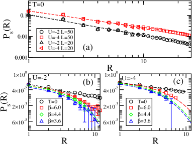
Figure 3: (Color online) (a) $P_{s}(R)$ versus $R$ for different $U$ values and for two lattice sizes $N=50$ and $N=20$, always at quarter filling, obtained from the ground state DMRG calculation. (b) $P_{s}(R)$ versus $R$ for $U=-2$ for a chain with $N=20$ sites as a function of $\beta$. The $T=0$ values scale as a power law. The $T>0$ values scale exponentially. Data points were deleted beyond a certain $R$; the text explains. (c) Same as (b) for $U=-4$. For the values of all exponents see table 2.

$U$	$20\times 1$	$50\times 1$	$d=1$	$\beta=6.0$	$\beta=4.4$	$\beta=3.6$
-2	1.055	0.991	0.80	0.57	0.69	0.72	12%
-4	0.867	0.784	0.70	0.48	0.68	0.72	3%
-8	0.808	0.725	0.65	0.94	1.21	1.34	6%

Table 2: Columns 2 and 3 show exponents $\bar{\beta}$ for the power law fit done at $T=0$ in figure 3(a). Values of $\bar{\beta}$ at the thermodynamic limit in one dimension are indicated by $d=1$, and obtained from Figure 8 of reference Kawakami and Yang, 1991 at quarter filling. The next three columns show exponents $\gamma$ for the exponential fit done at $T>0$ for $N=20$ in figures 3(b) and (c). The last column is $100\times|1-6.0\times\gamma(6.0)/(4.4\times\gamma(4.4)|$.

Several caveats regarding the way exponents were obtained need to be noted. In these METTS simulations $\mu$ had to be fixed to yield a density approximate to quarter filling. Actual densities obtained were in the range 0.2 to 0.3 instead of exactly at 0.25. $P_{s}(R)$ at finite and, in particular, large temperatures has large statistical errors. The first five METTS were discarded due to convergence reasons, similar to the case in figure 1. Approximately 10 to 20 METTS were used for measurements, and multiple METTS series run starting from different and random CPSs. Most results were computed with a fixed and random collapse basis. A few controls were performed with computational runs with the bases changed at each collapse; discrepancies between the two collapse procedures fell within the error bars. For the purposes of fitting to an exponential, values beyond a certain $R$ were discarded when either (i) behavior became non-monotonic, or (ii) $P_{s}(R)$ became slightly negative. These two effects are due to statistical errors: In most cases, discarded points had errors—shown by the error bars in figure 3(b,c)—larger than their average values.

III.2.2 Non-local correlation

Let us now consider the non-local parity correlator for charge

$$O_{P}^{(s)}(r)=\langle\exp(2i\pi\sum_{j=i}^{i+r}S^{z}_{j})\rangle,$$ (4)

with $S^{z}_{i}=\frac{1}{2}(n_{i\uparrow}-n_{i\downarrow})$, which is discussed in Montorsi and Roncaglia(͑2012), and references therein. Figure 4 shows $O_{P}^{(s)}(r)$ vs $r$ at $T=0$ and at $T>0$, for chains of 20 sites at half filling, and for two values of $U$, as indicated.

In the $U<0$ case considered here the Luther-Emery phase is characterized by nonzero $O_{P}^{(s)}(r)$,Montorsi and Roncaglia(͑2012) and the transition is known to be of Berezinskii-Kosterlitz-Thouless (BKT) type. The non-local order parameter $O_{P}^{(s)}(r)$ remains finite even at $T>0$, as seen in the figure.

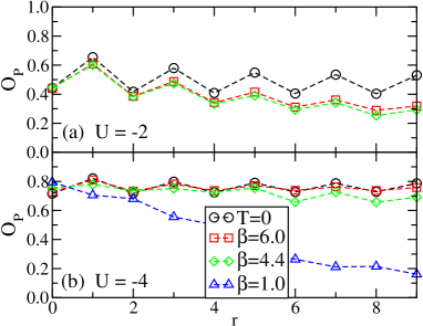
Figure 4: (Color online) $O_{P}^{(s)}(r)$ vs $r$ for chains of 20 sites at half filling and (a) $U=-2$ and (b) $U=-4$.

IV Summary and Outlook

A procedural description for the generation of METTS was presented, using the Krylov-space approach to perform the imaginary time evolution of the classical product states. The full open source code, input decks and additional computational details have been made available at https://web.ornl.gov/~gz1/papers/40/.Ince et al. (2012) By averaging over 100 to 200 METTS, global observables can be obtained with reasonable errors. Applied to local observables, in the example of the density in a site-dependent potential, the simulations converge to exact results as more series of METTS are added.

For an attractive Hubbard model on a chain, the application of the METTS algorithm verified the exponential decay of correlations—as opposed to the power law decay for the ground state. Or, conversely, the correct behavior of the exponents obtained with the METTS algorithm verified its feasibility. The exponents $\gamma$ are proportional to the temperature for low enough temperatures, as expected from rigorous bounds. A similar departure from power law at finite temperature has been observed for a spinless model with nearest and next-nearest neighbor interactions.Karrasch and Moore (2012)

These studies should set the stage for the further use of METTS in fermionic systems. We should envision using METTS to compute transition temperatures in models of pnictides superconductors, where, as mentioned before, spin flipping terms might preclude the use of quantum Monte Carlo methods due to the sign problem. One difficulty will be the vanishing of superconducting correlations in two dimensional systems,Mermin and Wagner (1966); Kosterlitz and Thouless(͑1973͒) ; Paiva et al. (2004) a difficulty that could be overcome by explicitly breaking symmetries with an anisotropic term.Gelfert and Nolting (2001) Multiple orbital models, as needed for pnictides superconductors, have larger Hilbert spaces, and would require longer runs. Let us not forget, however, that estimating exponents (as was done in this work) has high demands in terms of accuracy. But for multi-orbital superconductors, computing transition temperatures would be the main interest and motivation, and computing transition temperatures—assuming a true second order transition is present—could be achieved with less measurements than needed for estimating exponents.