The dipole model Monte Carlo generator Sartre 1

Abstract

We present the Monte Carlo generator Sartre  for simulating diffractive exclusive vector meson production and DVCS in electron-proton, electron-ion, and hadron-hadron collisions.

Program Summary

Program Title: Sartre 1.0

Authors: Tobias Toll, Thomas Ullrich

Licensing provisions: GPL version 2

Programming language: C/C++

Computer for which the program is designed and others on which it is operable: Any with standard C/C++ compiler. Tested on Linux and MacOS.

Separate documentation available via: https://code.google.com/p/sartre-mc/

Nature of physical problem: Simulate diffractive exclusive vector meson and deeply virtual Compton scattering (DVCS) production in electron-nucleus scattering where the exchanged virtual photon interacts coherently with a large region of the nucleus. To calculate the cross section correctly it has to be averaged over all possible configurations of nucleon positions within the nucleus.

Method of solution: To make an arithmetic average of the quantum mechanical amplitude over nucleon configurations numerically and store the result in look-up tables.

Implemented processes: The following processes can be simulated:

$$e+p\rightarrow e^{\prime}+V+p^{\prime}$$

$$e+A\rightarrow e^{\prime}+V+A^{\prime}$$

$$p+p\rightarrow p^{\prime}+V+p^{\prime}$$

$$p+A\rightarrow p^{\prime}+V+A^{\prime}$$

$$A+A\rightarrow A^{\prime}+V+A^{\prime}$$

where $V$ is a $J/\psi$, $\phi$, or $\rho$ vector meson, or a real photon (DVCS). All processes are mediated by a virtual photon and a pomeron.

The present version is applicable for these processes at future electron-hadron colliders, such as the EIC and the LHeC, as well as HERA, RHIC, and the LHC.

Restrictions to physics problem: The program is reliable for process at $x_{I\!\!P}<10^{-2}$, and large $\beta=x/x_{I\!\!P}$.

Other Programs used: ROOT and GSL for numeric algorithms and other various tasks throughout the program. BOOST for multi-threaded integration (optional), GEMINI++ for nuclear break-up and CUBA for multidimensional numerical integration (the latter two supplied with the program package). Uses cmake for building and installing.

Unusual feature: None

Running time: On a MacBook Pro with a 2.66 GHz Intel Core i7 processor, event generation takes $\sim 0.1$ ms/event without correction and nuclear breakup, $\sim 0.2$ ms/event with the recommended corrections switched on, and $\sim 6$ ms/event when running with corrections and nuclear breakup.

Download of the program: http://code.google.com/p/sartre-mc/

LONG WRITE-UP

1 Introduction

The dipole model has been very successful in describing exclusive diffraction at HERA, and is presently the most common approach at small $x$. It describes the interaction between the electron and the proton by letting the virtual photon split into a quark-anti-quark pair, which forms a color dipole. This dipole subsequently interacts with the proton in the proton’s rest frame. The dipole model in its present form was suggested by Golec-Biernat and Wüsthoff (GBW) [1, 2], who observed that a simple ansatz of the dipole model, integrated over impact parameter, was able to simultaneously describe the total inclusive and diffractive cross sections, the latter of which the collinear DGLAP formalism underestimates severely. The GBW model contains saturation in the small $x$ regime in a natural way. However, the GBW model fails at describing the high $Q^{2}$ scaling violation observed in the inclusive cross section measured at HERA, something the DGLAP formalism is able to describe perfectly. Bartels, Golec-Biernat, and Kowalski (BGBK) therefore included an explicit DGLAP gluon distribution into the dipole formalism [3], taken at a scale directly linked to the dipole size. The BGBK model replicates the GBW model where it is applicable and also manages to describe the $Q^{2}$ dependence of the cross sections. However, this approach still integrates out the impact parameter dependence of the interaction, without which the $t$-dependence of the cross section is undetermined. The impact parameter dependence was introduced in the dipole model by Kowalski and Teaney [16] and then modified to also include exclusive processes by Kowalski, Teaney, and Motyka [18]. This dipole model goes by the name bSat (or sometimes IPSat). Kowalski and Teaney also introduced a linearized version of bSat, called bNonSat, in order to separate and thus isolate non-linear effects to the cross sections [16].

In a recent paper we described in detail how the bSat and bNonSat models can be extended to also describe DIS with heavy nuclei [4]. We have implemented the bSat and bNonSat dipole models, for both protons and nuclei, into a Monte Carlo event generator named Sartre, which is the focus of this paper.

The main motivation for creating Sartre comes as a part of the effort to realize a future electron-ion collider (EIC) [5]. While the legacy of HERA is a plethora of physics generators describing all aspects of electron-hadron collisions (e.g. PYTHIA6 [6], HERWIG++ [7], LEPTO [8], PEPSI [9], RAPGAP [10], ARIADNE [11], CASCADE [12], SHERPA [13]), there is a dearth of such generators describing electron-ion collisions. The only exception known to us is DPMJET-III [14], which however is limited to photo-production ($Q^{2}=0$) and high-mass diffractive dissociation including multiple jet production. One of the key measurements at an EIC is that of the spatial distribution of gluons at small $x$, which has never been studied experimentally. To obtain the spatial gluon distribution, one measures the diffractive cross section, $d\sigma/dt$, at low-$x$ over a large range of $t$. A non-trivial Fourier transform from momentum space to coordinate space provides then the desired source distribution $F(b_{T})$. However, a direct measurement of $t=(\textbf{p}-\mathbf{p}^{\prime})^{2}$ is not possible in $eA$ collisions since the scattered ion ($\mathbf{p}^{\prime}$) is not sufficiently well separated from the beam. The only processes that allow access to $t$ with sufficiently high precision are exclusive diffractive processes, such as exclusive vector-meson production and deeply virtual Compton scattering (DVCS). Here $t$ can be calculated from the measured vector meson (or photon), the scattered electron, and the known beam energies. From an experimental standpoint this is rather challenging measurement that requires a carefully designed detector, making detailed simulations of the underlying physics an imperative.

There is presently one class of events at existing hadron collider experiments (RHIC and LHC) that can be described by Sartre: those of ultraperipheral collisions (UPC) between hadrons. In these events, the impact parameter between the colliding hadrons is so large that the long-range electro-magnetic force dominates over the short-ranged strong force. Therefore, these interactions are mediated by a virtual photon, and can thus potentially be described by the dipole model.

The program is named after the existentialist philosopher Jean-Paul Sartre. According to existentialism, existence comes before essence, but Sartre mentions the following important exception to that rule in a lecture held 1945 [15]:

If one considers an article of manufacture as, for example […] a paper-knife – one sees that it has been made by an artisan who had a conception of it; and he has paid attention, equally, to the conception of a paper-knife and to the pre-existent technique of production which is a part of that conception. […]Thus the paper-knife is at the same time an article producible in a certain manner and one which, on the other hand, […] serves a definite purpose, for one cannot suppose that a man would produce a paper-knife without knowing what it was for. Let us say, then, of the paperknife that its essence […] precedes its existence. […]Here, then, we are viewing the world from a technical standpoint, and we can say that production precedes existence.

The purpose of Sartre is to provide simulations of events at an electron-ion collider, not yet in existence. Therefore, one may say, Sartre provides the artisan’s pre-conception of the essence of an EIC, which is a necessary guidance for the construction of the machine and its detectors.

The paper is organized as follows: In section 2 we give a description of the dipole models implemented in Sartre. In section 3, the program is given an overview description. Finally, in section 4, we give an example of a user program running Sartre.

2 The dipole model in $ep$ and $e$A

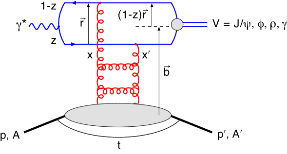
Figure 1: A schematic view of the dipole model and its variables. See text for details.

The amplitude for producing an exclusive vector meson or a real photon diffractively in an interaction between a virtual photon and a proton can be written as:

$$\mathcal{A}_{T,L}^{\gamma^{*}p}(x_{I\!\!P},Q,\Delta)=i\int{\rm d}r\int\frac{{\rm d}z}{4\pi}\int{\rm d}^{2}{\bf b}\left[\left(\Psi^{*}_{V}\Psi\right)(r,z)\right]2\pi rJ_{0}([1-z]r\Delta)e^{-i{\bf b}\cdot{\Delta}}\frac{{\rm d}\sigma_{q\bar{q}}^{(p)}}{{\rm d}^{2}{\bf b}}(x_{I\!\!P},r,{\bf b}),~{}~{}$$ (2)

where $r$ is the dipole’s size, ${\bf b}$ its impact parameter in relation to the proton’s mass center, and $z$ is the momentum fraction of the dipole taken by the quark. The variable $x_{I\!\!P}$ is the pomeron’s momentum fraction of the proton, $Q^{2}$ the virtuality of the photon, and $\Delta$ the virtuality of the . The virtual photon is either longitudinally or transversely polarized, denoted by $L$ and $T$, respectively. $J_{0}$ is a Bessel function and $\left(\Psi^{*}_{V}\Psi\right)(r,z)$ is the wave-function overlap between the incoming virtual photon and the outgoing vector-meson or real photon.

The proton dipole cross section is given by:

$$\frac{{\rm d}_{q\bar{q}}^{(p)}}{{\rm d}^{2}{\bf b}}(x_{I\!\!P},r,{\bf b})=2\mathcal{N}^{(p)}(x_{I\!\!P},r,{\bf b})=2\left[1-\Re(S)\right]$$ (3)

where $\mathcal{N}^{(p)}$ is the scattering amplitude of the proton. We only use the real part of the $S$-matrix. In the bSat model the scattering amplitude is:

$$\mathcal{N}^{(p)}=1-\exp\left(-\frac{\pi^{2}}{2N_{C}}r^{2}\alpha_{\rm S}(\mu^{2})x_{I\!\!P}g(x_{I\!\!P},\mu^{2})T(b)\right)$$ (4)

where $\mu^{2}=4/r^{2}+\mu_{0}^{2}$ and $\mu_{0}^{2}$ is a cut-off scale in the DGLAP evolution of the gluons $xg(x,\mu^{2})=A_{g}x^{-\lambda_{g}}(1-x)^{5.6}$. The impact parameter dependence is introduced through the proton’s profile function $T(b)=1/(2\pi B_{G})\exp(-b^{2}/(2B_{G}))$. All parameter values are determined through fits to HERA data [18], and are found to be $B_{G}=4~{}{\rm GeV}^{-2}$, $\mu_{0}^{2}=1.17$ GeV², $\lambda_{g}=0.02$, and $A_{g}=2.55$. Also, the four lightest quark masses are treated as parameters in the model, and are taken to be: $m_{u}=m_{d}=m_{s}=0.14$ GeV, $m_{c}=1.4$ GeV.

The nuclear scattering amplitude is constructed from that of the proton:

$$1-\mathcal{N}^{(A)}(x_{I\!\!P},{\bf r},{\bf b})=\prod_{i=1}^{A}\left(1-\mathcal{N}^{(p)}(x_{I\!\!P},{\bf r},|{\bf b}-{\bf b}_{i}|)\right)$$ (5)

where ${\bf b}_{i}$ is the position of each nucleon in the nucleus in the transverse plane. We distribute the nucleons according to the Woods-Saxon function projected onto the transverse plane. Combining equations (3), (4), and (5), the bSat dipole cross section for $\gamma^{*}$A becomes:

$$\frac{1}{2}\frac{{\rm d}\sigma_{q\bar{q}}^{(A)}}{{\rm d}^{2}{\bf b}}(x_{I\!\!P},r,{\bf b},\Omega_{j})=1-\exp\bigg{(}-\frac{\pi^{2}}{2N_{C}}r^{2}\alpha_{S}(\mu^{2})x_{I\!\!P}g(x_{I\!\!P},\mu^{2})\sum_{i=1}^{A}T(|{\bf b}-{\bf b}_{i}|)\bigg{)}$$ (6)

where $\Omega_{j}=\{{\bf b}_{1},{\bf b}_{2},\dots,{\bf b}_{A}\}$ represents a specific Woods-Saxon configuration of nucleons.

In $ep$ the diffractive cross section is given by the absolute square of the amplitude:

$$\frac{{\rm d}\sigma^{\gamma^{*}p}_{T,L}}{{\rm d}t}=\frac{1}{16\pi}\left|\mathcal{A}^{\gamma^{*}p}(x_{I\!\!P},Q^{2},t)\right|^{2}.$$ (7)

In $e$A one has to average the squared amplitude over all possible nucleon configurations $\Omega$:

$$\frac{{\rm d}\sigma^{\gamma^{*}A}_{T,L}}{{\rm d}t}=\frac{1}{16\pi}\left<\left|\mathcal{A}^{\gamma^{*}p}(x_{I\!\!P},Q^{2},t)\right|^{2}\right>_{\Omega}.$$ (8)

In $e$A there are two possible scenarios: either the interaction between the nucleus and the dipole is elastic, or it is inelastic, in which case the nucleus de-excites subsequent to the interaction by breaking up into color-neutral fragments. The first case is called coherent and the latter is called incoherent. According to the Good-Walker picture, the incoherent cross section is proportional to the variance of the amplitude:

$$\frac{{\rm d}\sigma_{\rm incoherent}}{{\rm d}t}=\frac{1}{16\pi}\bigg{(}\left<\left|\mathcal{A}(x_{I\!\!P},Q^{2},t,\Omega)\right|^{2}\right>_{\Omega}-\left|\left<\mathcal{A}(x_{I\!\!P},Q^{2},t,\Omega)\right>_{\Omega}\right|^{2}\bigg{)}$$ (9)

where the second term on the R.H.S. is the coherent part of the cross section. To calculate the diffractive cross sections for incoherent and coherent interaction therefore becomes a matter of calculating the second and first moments of the amplitude respectively.

For the first moment there is a closed expression for the average of the dipole cross section [16]:

$$\left<\frac{{\rm d}\sigma_{q\bar{q}}}{{\rm d}^{2}{\bf b}}\right>_{\Omega}=2\left[1-\left(1-\frac{T_{A}({\bf b})}{2}\sigma^{p}_{q\bar{q}}\right)^{A}\right]$$ (10)

where $\sigma^{p}_{q\bar{q}}$ is the $ep$ dipole cross section, eq. (3), integrated over the impact parameter, and $T_{A}$ is the spatial density profile of ions which is taken to be the Woods-Saxon potential in transverse space.

For the second moment of the amplitude, no analytical expression exists. We define the average of an observable $\mathcal{O}(\Omega)$ over nucleon configurations $\Omega_{i}$ by:

$$\left<\mathcal{O}\right>_{\Omega}=\frac{1}{C_{\rm max}}\sum_{i=1}^{C_{\rm max}}\mathcal{O}(\Omega_{i}).$$ (11)

For a large enough number of configurations $C_{\rm max}$ the sum on the R.H.S. will converge to the true average. For the total diffractive cross section one gets:

$$\frac{{\rm d}\sigma^{\gamma^{*}{\rm A}}}{{\rm d}t}(x_{I\!\!P},Q^{2},t)=\frac{1}{16\pi}\frac{1}{C_{\rm max}}\sum_{i=1}^{C_{\rm max}}\left|\mathcal{A}(x_{I\!\!P},Q^{2},t,\Omega_{i})\right|^{2}.~{}~{}~{}~{}$$ (12)

For large $|t|$, the variance of the amplitude is several orders of magnitude larger than the average. This means that the convergence of the sum in eq. (11) becomes extremely slow. For the first moment we therefore use eq. (10). For the second moment we have shown in [4] that 500 configurations give a good convergence.

2.1 The non-saturated dipole model

In order to separate saturation from other small-$x$ effects, a linearized version of the dipole model, called the bNonSat model [16], is implemented in Sartre. It is obtained by linearizing the dipole cross section of the bSat model. By doing so the gluon density becomes unsaturated for small $x$ and for large dipole sizes $r$.

In the proton case, the bNonSat dipole cross section is obtained by keeping the first term in the expansion of the exponent in the bSat dipole cross section [16]:

$$\frac{{\rm d}\sigma_{q\bar{q}}^{(p)}}{{\rm d}^{2}b}=\frac{\pi^{2}}{N_{C}}r^{2}\alpha_{s}(\mu^{2})x_{I\!\!P}g(x_{I\!\!P},\mu^{2})T(b)$$ (13)

In the case of a nucleus the dipole cross section becomes [4]:

$$\frac{{\rm d}\sigma_{q\bar{q}}^{(A)}}{{\rm d}^{2}b}=\frac{\pi^{2}}{N_{C}}r^{2}\alpha_{s}(\mu^{2})x_{I\!\!P}g(x_{I\!\!P},\mu^{2})\sum_{i=1}^{A}T(|{\bf b}-{\bf b}_{i}|)$$ (14)

and the coherent part of the bNonSat cross section can be obtained by the average [4]:

$$\left<\frac{{\rm d}\sigma_{q\bar{q}}^{(A)}}{{\rm d}^{2}b}\right>_{\Omega}=\frac{\pi^{2}}{N_{C}}r^{2}\alpha_{s}(\mu^{2})x_{I\!\!P}g(x_{I\!\!P},\mu^{2})AT_{A}(b)$$ (15)

while the second moment of the amplitude is averaged over nucleon configurations as above.

2.1.1 Corrections to the dipole cross section

In the derivation of the dipole amplitude only the real part of the $S$-matrix is taken into account. The imaginary part of the scattering amplitude can be included by multiplying the cross section by a factor $(1+B^{2})$, where $B$ is the ratio of the imaginary and real parts of the scattering amplitude. It is calculated using [18]:

$$B=\tan\left(\lambda\frac{\pi}{2}\right),~{}{\rm where}~{}\lambda\equiv\frac{\partial\ln\left(\mathcal{A}_{T,L}^{\gamma*p\rightarrow Vp}\right)}{\partial\ln(1/x)}.$$ (16)

In the derivation of the dipole amplitude, the gluons in the two-gluon exchange in the interaction are assumed to carry the same momentum fraction of the proton or nucleus. To account for the cases where they carry different momentum fractions, a so-called skewness correction is applied to the cross section by multiplying it by a factor $R_{g}(\lambda)$, defined by [18]:

$$R_{g}(\lambda)=\frac{2^{2\lambda+3}}{\sqrt{\pi}}\frac{\Gamma(\lambda+5/2)}{\Gamma(\lambda+4)}$$ (17)

where $\lambda$ is defined in eq. (16).

These corrections are important for describing HERA data. Where the models are valid the corrections are typically around 60% of the cross section, with approximately 45% attributable to the skewness correction. The corrections grow dramatically in the large-$x$ range outside the validity of the models, where $x_{I\!\!P}>10^{-2}$.

2.2 Calculating Cross sections

The total diffractive differential cross section is:

$$\frac{{\rm d}^{3}\sigma_{\rm total}}{{\rm d}Q^{2}{\rm d}W^{2}{\rm d}t}=\sum_{T,L}\frac{R_{g}^{2}(1+B^{2})}{16\pi}\frac{{\rm d}n_{T,L}^{\gamma}}{{\rm d}Q^{2}{\rm d}W^{2}}\left<|\mathcal{A}_{T,L}|^{2}\right>_{\Omega}~{}~{}$$ (18)

where ${\rm d}n_{T,L}^{\gamma}/{\rm d}Q^{2}{\rm d}W^{2}$ is the flux of transversely and longitudinally polarized virtual photons, and the average over configurations $\Omega$ is defined in eq. (11). The photon flux may be that from an electron, as in the case of $ep$ and $e$A collisions, but it may also emanate from protons or ions in the case of ultraperipheral collisions (UPC) in hadron colliders, as described in e.g. [19].

The coherent part of the cross section is:

$$\frac{{\rm d}^{3}\sigma_{\rm coherent}}{{\rm d}Q^{2}{\rm d}W^{2}{\rm d}t}=\sum_{T,L}\frac{R_{g}^{2}(1+B^{2})}{16\pi}\frac{{\rm d}n_{T,L}^{\gamma}}{{\rm d}Q^{2}{\rm d}W^{2}}\left|\left<\mathcal{A}_{T,L}\right>_{\Omega}\right|^{2}~{}~{}$$ (19)

while the incoherent part is the difference between the total and coherent cross sections. The incoherent part directly gives the probability for the nucleus breaking up.

For the the second moment of the amplitude, for each nucleon configuration $\Omega_{i}$, one needs to calculate the integral:

$$\mathcal{A}_{T,L}(Q^{2},\Delta,x_{I\!\!P},\Omega_{i})=\!\int r{\rm d}r\frac{{\rm d}z}{2}{\rm d}^{2}{\bf b}\left(\Psi^{*}_{V}\Psi\right)_{T,L}(Q^{2},r,z)J_{0}([1-z]r\Delta)e^{-i{\bf b}\cdot{\bf\Delta}}\frac{{\rm d}\sigma_{q\bar{q}}}{{\rm d}^{2}{\bf b}}(x_{I\!\!P},r,{\bf b},\Omega_{i})~{}~{}~{}~{}~{}$$ (20)

where the dipole cross section is defined in eq. (6) for bSat and in eq. (14) for bNonSat. For $e$A, there is no angular symmetry in ${\bf b}$ which makes this integral a complex number. We average over 500 nucleon configurations, giving 1000 such integrals for each point in phase-space (500 for each polarization).

For the first moment of the amplitude, the integral to calculate is:

$$\left<\mathcal{A}_{T,L}(Q^{2},\Delta,x_{I\!\!P})\right>_{\Omega}\!=\!\int\pi r{\rm d}r{\rm d}zb{\rm d}b\left(\Psi^{*}_{V}\Psi\right)_{T,L}(Q^{2},r,z)J_{0}([1-z]r\Delta)J_{0}(b\Delta)\left<\frac{{\rm d}\sigma_{q\bar{q}}}{{\rm d}^{2}{\bf b}}\right>_{\Omega}(x_{I\!\!P},r,b)$$ (21)

where the average in the last term is defined in eq. (10) for bSat and in eq. (15) for bNonSat.

The dipole models described here are only valid for small values of $x_{I\!\!P}<10^{-2}$ and not too small values of $\beta\equiv x/x_{I\!\!P}$. If $\beta$ becomes too small the $q\bar{q}$ dipole becomes unphysically large [20]. To rectify this one would need to include higher Fock state dipoles, such as $q\bar{q}g$. However, this growth has no effect on the actual production cross sections (eq. (18) and (19)) due to the implicit cut-off of the wave-overlap at already moderate radii as discussed in [4]. To nevertheless protect against this unphysical behavior, we introduce a cut-off in the dipole radius of $r<3$ fm for protons and $r<3R_{0}$ for nuclei, where $R_{0}$ is the nucleus’ radius given in the Woods-Saxon parametrization. We varied the cut-off in a wide range and did not observe any changes in the resulting cross sections.

3 Description of the program

Sartre is not a stand-alone program but consists of a set of C++ classes and C-functions that together form the Application Programming Interface (API). Although the classes are primarily designed to provide tools to generate events they also can be used to calculate cross sections or study model dependencies.

In this section we will give an overview of most of the classes in Sartre and how they can be used. We will give, by means of example programs, an overview on how to deploy them to generate amplitude look-up tables, cross sections, and events.

The master equation of Sartre is the total cross section described in eq. (18). This cross sections is used as a probability density function (PDF) from which a phase-space point $(Q^{2},W^{2},t)$ is drawn for each event. The phase-space point together with the given beam energies fully determines the final state, except for the azimuthal angle of the vector meson, which we distribute uniformly.

To determine the diffractive cross section in $e$A at a point in phase-space a complex 4-dimensional integral needs to be calculated for 500 nuclear configurations. The fact that 1000 (500 for each polarization) such 4-dimensional integrals have to be calculated at each point in phase-space makes efficient event generation essentially impossible. The only viable approach is to compute the first and second moments of the amplitudes separately and store the result in 3-dimensional lookup-tables in $Q^{2}$, $W^{2}$, and $t$. This has to be done for each nuclear species, each final-state vector meson and DVCS, each polarization, as well as for each dipole model (bSat or bNonSat). This requires a set of four look-up tables:

$$\left<\mathcal{A}_{T}\right>_{\Omega}(Q^{2},W^{2},t),~{}\left<\mathcal{A}_{L}\right>_{\Omega}(Q^{2},W^{2},t),~{}\left<|\mathcal{A}_{T}|^{2}\right>_{\Omega}(Q^{2},W^{2},t),~{}{\rm and}~{}\left<|\mathcal{A}_{L}|^{2}\right>_{\Omega}(Q^{2},W^{2},t)$$ (22)

where $L$ and $T$ denote longitudinal and transverse polarization of the photon, respectively. These look-up tables contains all the physics of the dipole-models described in section 2.

In addition we also provide tables for calculating the phenomenological corrections described in eqs. (16) and (17). They hold the values of $\lambda$ defined in eq. (16) for each $Q^{2}$, $W^{2}$ and $t$ bin matching those of the amplitude tables. We provide one table for each species of vector meson. However, we also put a fall back solution in place that derives $\lambda$ from the proton amplitude tables should the lambda table not be available.

Hence, the classes in Sartre have to accomplish two tasks. The first is the generation of the look-up tables for the first and second moments of the amplitude, the second is the actual generation of the events using the look-up tables to calculate a cross section from which the PDF is constructed. Without further features enabled (such as nuclear break-up), the event generation can simulate around a million events in a matter of 3 minutes on our laptop computers.

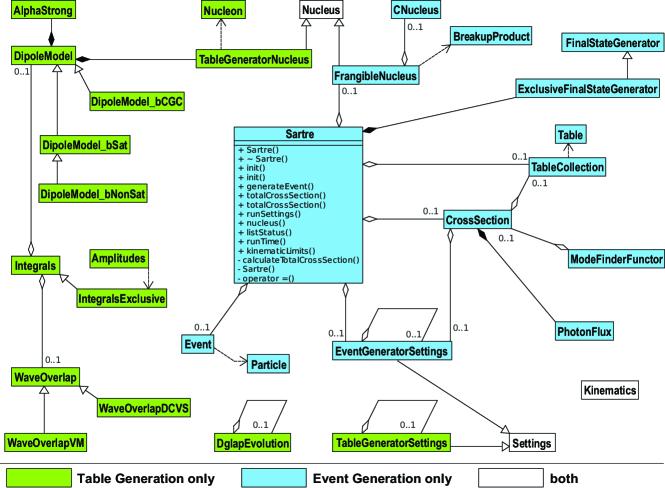
Figure 2: Class Diagram of the most important classes used in Sartre. Operations and attributes are omitted for clarity, except for class Sartre where all public operations are listed. Classes shown in green are used only for the table generation, classes in blue only for event generation. We use Unified Modeling Language.

To generate events the user has to provide a main program and optionally a runcard, i.e., a text file with instructions read by Sartre, that define various parameters such as beam energies, what dipole model to use, what vector meson species to generate, the number of events, and much more. The overall controlling class is Sartre while the defined parameters are managed by EventGeneratorSettings, a singleton class.

Figure 2 depicts the Unified Modeling Language (UML) diagram of the most important classes and their relations. Class Sartre is shown with all public operations listed while for all other classes they are omitted for clarity.

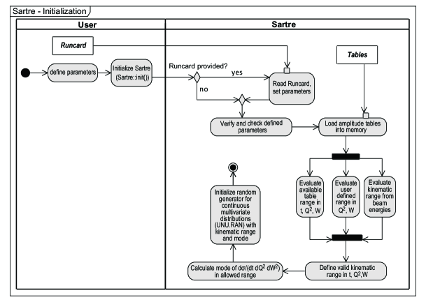
Figure 3: Activity diagram showing the process for initializing Sartre for event generation.

In the users main program the first step is to create an instance of Sartre and initialize all parameters. The user can provide all parameters either programatically or through a runcard. The UML activity diagram in Fig. 3 illustrates the initialization process. At the end, the following tasks are accomplished: (i) the amplitude look-up tables are read and stored in memory, (ii) the actual kinematic range in $Q^{2}$, $W$, and $t$ is determined from the table limits, the beam energies, and the user input, and (iii) the random number generator (UNU.RAN) is initialized using a functor that computes the cross section for a given $Q^{2}$, $W$, and $t$, using the stored amplitude tables. To initialize UNU.RAN the mode of the PDF has to be computed, which is numerically challenging since the mode typically lies at the border of the kinematically valid range. During the initialization the instance of Sartre prints the status and general information depending on the level of verbosity set by the user. Once initialized the user can only change parameters that are related to event processing; changing parameters that are related to kinematic range or physics processes will have no effect.

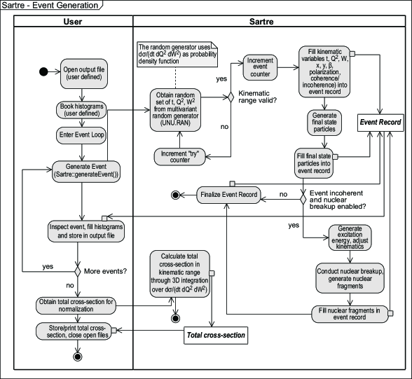
Figure 4: Activity diagram showing the process of event generation using Sartre.

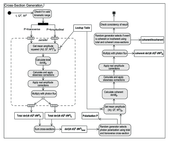
Figure 5: Activity diagram depicting the calculation of the cross section in a given kinematic range.

Once Sartre is initialized, the initialized instance can be used for generating events. Figure 4 shows the UML activity diagram of the overall process while Figure 5 depicts the actual process of deriving the cross section(s). From the PDF, the random generator (UNU.RAN) provides a phase-space point in $Q^{2}$, $W$, and $t$. However, UNU.RAN internally operates on rectangular borders exceeding in certain areas of the phase space the limits of the kinematic acceptance. Therefore additional kinematic checks have to be conducted. If the event is rejected, a new one is automatically generated. The difference between “tried” and generated events is typically small ($<1\%$). The values of $Q^{2}$, $W$, and $t$, together with the beam energies and masses of the incoming and outgoing particles fully define the final state which is calculated by the final state generator (class ExclusiveFinalStateGenerator), giving 4-momenta of all out-going particles. By comparing the incoherent and coherent cross sections in the event, it is then decided probabilistically whether the nucleus subsequently breaks up or not. If it does, the outgoing nucleus may then fragment by the GEMINI++ intra nuclear cascade [21]. GEMINI++ is a statistical model code which describes the nuclear de-excitation, providing the break-up products from neutrons up to the heaviest fragments. It needs as input the excitation energy $E^{*}$ of the nucleus, which is given by:

$$E^{*}=(M_{Y}-m_{n})\cdot A$$ (23)

We assume that the diffractive mass $M_{Y}$ is distributed according to:

$$\frac{{\rm d}N}{{\rm d}M_{Y}^{2}}\propto\frac{1}{M_{Y}^{2}}.$$ (24)

Note that $M_{Y}$ cannot be uniquely determined from kinematics alone.

Once the events have been generated one typically wants to calculate the total cross section for the kinematic range in question in order to allow the absolute normalization of the generated spectra. This can be done independently of the event generation. Sartre uses the Adaptive multi-dimensional algorithm in ROOT [22] and GSL [23] to integrate the cross section over a valid kinematic range. If that fails, the fall-back option is VEGAS.

What follows is a description of how to obtain Sartre, and of the different components of the program.

3.1 Installation

The source-code is available at: http://code.google.com/p/sartre-mc/ The complete source-code including the tables and documentation can be downloaded as a tar ball (recommended) or alternatively extracted form the subversion repository.

Unpack the downloaded tar ball: tar -xzvf sartre-$<$version$>$.tgz

The main directory (sartre) contains a INSTALL.HTML file with detailed instruction how to build and set up Sartre using the provided cmake files.

Sartre is by default installed in /usr/local/sartre containing the libraries (libs/), the include files (include/), the html documentation (docs/), the tables (tables/), GEMINI++ ( gemini/), a directory with various example programs (examples/), and a directory with binaries (bin/) that contains tools to query and browse the amplitude tables. The installation directory can be set by the user via cmake command line options.

Sartre requires two additional packages to be installed: ROOT and the GNU Scientific Library (GSL). ROOT must contain the Unuran and MathMore components.

3.2 Enumerations

Table 1 shows a list of the few enumerations that are used throughout in Sartre.

Enumeration	Values
DipoleModelType	bSat, bNonSat, bCGC
GammaPolarization	transverse, longitudinal
AmplitudeMoment	mean_A, mean_A2, lambda_A
DiffractiveMode	coherent, incoherent

Table 1: A list of enumerations used throughout Sartre to identify the dipole model in use, the polarization of the virtual photon, which moment of the amplitude is being used and whether the event is coherent or incoherent.

3.3 A description of classes

We here give a description of those classes of the Sartre API which we deem to be most relevant for the user.

3.3.1 Class Sartre

Sartre is the central class of the event generation. It provides methods to initialize, control and run the even generator. It can also calculate cross section in a kinematic range. At a minimum the user needs to invoke two methods:

1. bool Sartre::init(char* runcard_file)

2. Event* Sartre::generateEvent()

where runcard_file is the name of the text file containing the run parameters (the runcard), and Event is the class holding the event record.

3.3.2 Class Event

The class Event holds the complete event record. The user has the option to print the event record. The event record contains the 4-momenta of all particles involved in the event, as well as the event’s kinematic variables $Q^{2}$, $W$, $t$, $x$, $x_{I\!\!P}$, $B$, $s$, $y$, the polarization of the virtual photon, whether the event is coherent or incoherent and the number of the event. The event record also has information on parent and daughter particle relationships. If nuclear breakup is enabled it will also hold the nuclear fragments and their 4-momenta.

3.3.3 Class BreakupProduct

BreakupProduct holds information about the fragments created by nuclear breakup in incoherent $e$A collisions. It holds the results of GEMINI++, the Monte Carlo used to describe the nuclear breakup. Each fragment from GEMINI++ is stored as a BreakupProduct structure and kept in a vector that is later passed and stored in the event record if nuclear breakup is switched on (via a runcard or programmatically). The emission time of the fragment is in units of $10^{-21}$ seconds since the creation of the compound nucleus in the nucleus rest frame. This unit is common in nuclear physics and we left it as provided by GEMINI++. Note that the 4-momenta are already boosted into the Sartre lab frame and are not expressed per nucleon here as it is done in the main event record.

3.3.4 Class Nucleus

The Nucleus class contains the necessary information about the nucleus, such as name, radius, spin, mass as well as the referring Woods-Saxon distribution to describe its density as a function of impact parameter. This class is used in the generation of the amplitude look-up tables, while a derived class FrangibleNucleus is used for event generation in class Sartre. The user does not have to care about the class or its initialization since it is handled internally in Sartre. However, it is always available through a call of Sartre::nucleus().

At the moment this class is able to describe the following nuclei: proton (1), oxygen (16), aluminum (27), calcium (40), copper (63), cadmium (110), gold (197), and lead (208).

3.3.5 Class Kinematics

The Kinematics class contains functions that calculate kinematic variables out of other variables. It contains functions for calculating the variables $x$, $y$, $s$, $W^{2}$, $x_{I\!\!P}$. It also contains the static beam particle 4-vectors and functions that calculate the kinematically allowed limits of $Q^{2}$, $W^{2}$, and $t$. Kinematics also contains a method to conduct an overall thorough check of the event kinematics. This function is invoked in several places to guarantee the numeric integrity of the generated events.

3.3.6 Class Particle

The Particle class contains all information needed to describe any particle used in Sartre. The particles are stored in an internal list in the Event class. It is a lightweight class without any member functions and all data members are public. The data members hold information on the particle’s status (stable or decayed), 4-momentum, parent particle(s), and daughter particle(s). Each particle is uniquely identified by an index number.

Note that momentum and energy of nuclei are always expressed as per-nucleon.

3.3.7 Class EventGeneratorSettings

The main API for event generation is class Sartre. However, Sartre does not handle the setup parameters at all but defers that job to the “Settings” classes. These classes are not only simple containers for parameters but provide lots of functionality to load, print, and manage parameters and also provide particle parameter lookup features. The basic functionality is provided by the Settings class, inherited by the EventGeneratorSettings class. For creating the amplitude table a separate class needs to be used (TableGeneratorSettings). EventGeneratorSettings only handles parameters needed for generating events and for calculating cross sections.

EventGeneratorSettings is a singleton class, i.e., only one instance exists at any time. One can always obtain the actual instance using the static EventGeneratorSettings::instance() method.

EventGeneratorSettings (via Settings) also provides the ”runcard” mechanism, that is the possibility to store all parameters to run Sartre, in a text file (the runcard) and read them in.

Parameters managed by EventGeneratorSettings can be set and used via access functions. Each access function has an equivalent runcard name.

3.3.8 Class TableGeneratorSettings

Inherits from Settings. Handles the settings for running the generator of look-up tables. Provides information such as which dipole model to use, in which kinematical limits and how to bin the lookup tables.

3.3.9 Class ExclusiveFinalStateGenerator

Calculates the final state given the phase-space point $(t,Q^{2},W^{2})$ and beam energies. The final state is stored in the event record (class Event).

3.3.10 Class Amplitudes and Class Integrals

The Amplitudes class calculates the quantities $\left<\left|\mathcal{A}^{\gamma^{*}p}_{L,T}\right|^{2}\right>_{\Omega}(W^{2},Q^{2},t)$ and $\left<\mathcal{A}^{\gamma^{*}p}_{L,T}\right>_{\Omega}(W^{2},Q^{2},t)$ at a given point in phase space. In Sartre it is used by the table generator and the result is stored in look-up tables. The integrations are performed by the Integrals class. There is an option to calculate the integrals for different nuclear configurations on parallel threads, using the BOOST library [25]. The integrations are using the CUBA library.

3.3.11 Class Table

This is a class of functions for creating a new look-up table of the amplitude momenta, or to read information from an existing look-up table. How tables are stored and read is described in further detail in A.

We provide a program “tableInspector” to inspect and browse the tables. It can be used either for getting basic information about the table, such as binning and ranges, but also to get detailed information about the content in each bin.

We also provide a program called “tableMerger” which can merge some tables into one combined table. This is very useful when one creates parts of a table in parallel on different computing nodes and then merge them into one table. For tableMerger to work, the granularities of the tables have to match, as well as the ranges, in two out of the three dimensions.

There are also tables which stores the values of $\lambda$ described in eq. (16). These tables are used by Sartre to calculate the real part and skewness corrections to the cross sections.

3.3.12 Class TableCollection

Several look-up tables may exist for a certain process. These tables may cover different kinematic regions and have different binning. The tables may also overlap in some kinematic regions. Sartre calculates the cross sections from TableCollection rather than Table. When Sartre calls TableCollection, it chooses from which of these tables to extract the information.

4 Example programs and runcards

In this sections we provide examples of user programs making use of the classes in Sartre. To generate events with Sartre, one first need lookup tables. There is a collection of such tables included in the package. Here we provide an example of how to use the event generator in Sartre, as well as providing an example program for how to generate the lookup tables.

The normal user is not expected to do the latter. Before generating lookup tables, the user need to produce a file containing nuclear configurations, which is produced with the example program createBSatBDependenceTable, and put it in a directory as given in the runcard.

4.1 Runcard for event generation

The following is an example of a runcard “sartreRuncard.txt” for generating $J/\psi$ mesons in electron-gold collisions:

⬇

//===================================================================

//

// Example Runcard for Sartre Event Generator.

//

// Comments start with a # or //

// Name and value are separated by a "=": name = value

// (alternatively ":" can be used as well)

//===================================================================

#

# Define beams [GeV]

#

eBeamEnergy = 20

hBeamEnergy = 100

# Define atom number of nucleus

A = 197

# Number of events and printout frequency

numberOfEvents = 1000

timesToShow = 20

# Set verbosity

verbose = false

verboseLevel = 1

# Rootfile or alternative file to store the generated events

rootfile = example.root

# Model parameters (jpsi=443, phi=333, rho=113, DVCS=22)

vectorMesonId = 443

dipoleModel = bSat

# Kinematic range min > max means no limits (given by table range)

# Q2 in GeV2, W in GeV

Q2min = 1

Q2max = 10

Wmin = 10

Wmax = 60

# Corrections

correctForRealAmplitude = true

correctSkewedness = true

#maxLambdaUsedInCorrections = 0.6

# Ultra Peripheral Collisions

# Simulate UPC?

UPC = false

# Atom number of photon emitting nucleus:

UPCA = 197

# Use Gemini++ to evaporate nucleus in incoherent event?

enableNuclearBreakup = true

maxNuclearExcitationEnergy = 0.5

# Random generator seed (if not given current time is used)

#seed = 2011987

4.2 Generating events

The following is an example of a user program “sartreMain” for generating events with Sartre, using a runcard for user input:

⬇

#include <iostream>

#include <cmath>

#include "TTree.h"

#include "TFile.h"

#include "Sartre.h"

using namespace std;

struct rootSartreEvent {

double t;

double Q2;

double x;

double s;

double y;

double W;

double xpom;

int iEvent;

int pol; // 0=transverse or 1=longitudinal

int dmode; // 0=coherent, 1=Incoherent

};

rootSartreEvent myRootSartreEvent;

int main(int argc, char *argv[])

{

//

// Check command line arguments

//

if (! (argc == 2 || argc == 3) ) {

cout << "Usage: " << argv[0] << " runcard [rootfile]" << endl;

return 2;

}

string runcard = argv[1];

//

// Create the generator and initialize it.

// Once initialized you cannot (should not) change

// the settings w/o re-initialing sartre.

//

Sartre sartre;

bool ok = sartre.init(runcard);

if (!ok) {

cerr << "Initialization of sartre failed." << endl;

return 1;

}

EventGeneratorSettings* settings = sartre.runSettings();

settings->list();

//

// ROOT file

//

string rootfile;

if (argc == 3)

rootfile = argv[2];

else

rootfile = settings->rootfile();

TFile *hfile = 0;

if (rootfile.size()) {

hfile = new TFile(rootfile.c_str(),"RECREATE");

cout << "ROOT file is ’" << rootfile.c_str() << "’." << endl;

}

//

// Setup ROOT tree

//

TLorentzVector *eIn = new TLorentzVector;

TLorentzVector *pIn = new TLorentzVector;

TLorentzVector *vm = new TLorentzVector;

TLorentzVector *eOut = new TLorentzVector;

TLorentzVector *pOut = new TLorentzVector;

TLorentzVector *gamma = new TLorentzVector;

TTree tree("tree","sartre");

tree.Branch("event", &myRootSartreEvent.t,

"t/D:Q2/D:x/D:s/D:y/D:W/D:xpom/D:

iEvent/I:pol/I:dmode/I");

tree.Branch("eIn", "TLorentzVector", &eIn, 32000, 0);

tree.Branch("pIn", "TLorentzVector", &pIn, 32000, 0);

tree.Branch("vm", "TLorentzVector", &vm, 32000, 0);

tree.Branch("eOut", "TLorentzVector", &eOut, 32000, 0);

tree.Branch("pOut", "TLorentzVector", &pOut, 32000, 0);

tree.Branch("gamma","TLorentzVector", &gamma, 32000, 0);

//

// Event generation

//

int nPrint;

if (settings->timesToShow())

nPrint = settings->numberOfEvents()/settings->timesToShow();

else

nPrint = 0;

unsigned long maxEvents = settings->numberOfEvents();

cout << "Generating " << maxEvents << " events." << endl << endl;

for (unsigned long iEvent = 0; iEvent < maxEvents; iEvent++) {

//

// Generate one event

//

Event *event = sartre.generateEvent();

if (nPrint && iEvent%nPrint == 0 && iEvent != 0) {

cout << "processed " << iEvent << " events" << endl;

}

//

// Print out (here only for the first few events)

//

if (iEvent < 4) event->list();

//

// Fill ROOT tree

//

myRootSartreEvent.iEvent = event->eventNumber;

myRootSartreEvent.t = event->t;

myRootSartreEvent.Q2 = event->Q2;

myRootSartreEvent.x = event->x;

myRootSartreEvent.y = event->y;

myRootSartreEvent.s = event->s;

myRootSartreEvent.W = event->W;

myRootSartreEvent.xpom = event->xpom;

myRootSartreEvent.pol =

event->polarization == transverse ? 0 : 1;

myRootSartreEvent.dmode =

event->diffractiveMode == coherent ? 0 : 1;

eIn = &event->particles[0].p;

pIn = &event->particles[1].p;

eOut = &event->particles[2].p;

pOut = &event->particles[6].p;

vm = &event->particles[4].p;

gamma = &event->particles[3].p;

tree.Fill();

}

//

// That’s it, finish up

//

double runTime = sartre.runTime();

hfile->Write();

cout << rootfile.c_str() << " written." << endl;

cout << "Total cross-section: " << sartre.totalCrossSection()

<< " nb" << endl;

sartre.listStatus();

cout << "CPU Time/event: " << 1000*runTime/maxEvents

<< " msec/evt" << endl;

return 0;

}

4.3 Output and Result from Event Generation

The following is the output resulting from running the example program “sartreMain” described in section 4.2:

/========================================================================\
|                                                                        |
|  Sartre, Version 1.10                                                  |
|                                                                        |
|  An event generator for exclusive diffractive vector meson production  |
|  in ep and eA collisions based on the dipole model.                    |
|                                                                        |
|  Copyright (C) 2010-2013 Tobias Toll and Thomas Ullrich                |
|                                                                        |
|  This program is free software: you can redistribute it and/or modify  |
|  it under the terms of the GNU General Public License as published by  |
|  the Free Software Foundation, either version 3 of the License, or     |
|  any later version.                                                    |
|                                                                        |
|  Code compiled on Aug 15 2013 09:56:29                                 |
|  Run started at Wed Dec 11 15:58:28 2013                               |
\========================================================================/
Runcard is ’/Users/tollto/sartre/paper-program/version5/generatorRuncardExample.txt’.
Hadron beam species: Au (197)
Hadron beam:   0Ψ0Ψ99.9956Ψ100Ψ(0.93827)
Electron beam: 0Ψ0Ψ-20Ψ20Ψ(0.000510999)
Dipole model: bSat
Process is e + Au -> e’ + Au’ + J/psi
Random generator seed: 1386795508
Sartre is initialized.


Run Settings:
                     userIntΨ0
                  userDoubleΨ0
                  userStringΨ
                 eBeamEnergyΨ20
                 hBeamEnergyΨ100
                           AΨ197
              numberOfEventsΨ1000
                 timesToShowΨ20
               vectorMesonIdΨ443
                 dipoleModelΨbSat
                       Q2minΨ1
                       Q2maxΨ10
                        WminΨ10
                        WmaxΨ60
     correctForRealAmplitudeΨtrue
           correctSkewednessΨtrue
        enableNuclearBreakupΨtrue
  maxLambdaUsedInCorrectionsΨ0.65
  maxNuclearExcitationEnergyΨ0.5
             applyPhotonFluxΨtrue
                     verboseΨfalse
                verboseLevelΨ0
                         UPCΨfalse
                        UPCAΨ197
                    rootfileΨexample.root
                        seedΨ1386795508

ROOT file is ’example.root’.
Generating 1000 events.

evt = 0           Q2 = 1.573         x = 1.104e-03
                   W = 37.734        y = 0.178
                   t = -0.007     xpom = 7.841e-03
                 pol = T          diff = coherent

   #          id   name       status    parents     daughters        px       py       pz        E           m
   0          11   e-              4    -     -      2     3      0.000    0.000  -20.000   20.000   5.110e-04
   1  1000791970   Au(197)         4    -     -      6     -      0.000    0.000   99.996  100.000       0.938
   2          11   e-              1    0     -      -     -      0.861   -0.743  -16.419   16.458   5.110e-04
   3          22   gamma           2    0     -      4     5     -0.861    0.743   -3.581    3.542      -1.254
   4         443   J/psi           1    3     -      -     -     -0.826    0.669   -2.809    4.314       3.097
   5         990   pomeron         2    3     3      6     -     -0.034    0.073   -0.772   -0.772      -0.082
   6  1000791970   Au(197)         1    1     5      -     -     -0.034    0.073   99.223   99.228       0.938

evt = 1           Q2 = 3.684         x = 2.582e-03
                   W = 37.734        y = 0.178
                   t = -0.007     xpom = 9.309e-03
                 pol = L          diff = coherent

   #          id   name       status    parents     daughters        px       py       pz        E           m
   0          11   e-              4    -     -      2     3      0.000    0.000  -20.000   20.000   5.110e-04
   1  1000791970   Au(197)         4    -     -      6     -      0.000    0.000   99.996  100.000       0.938
   2          11   e-              1    0     -      -     -      1.679    0.455  -16.387   16.479   5.110e-04
   3          22   gamma           2    0     -      4     5     -1.679   -0.455   -3.613    3.521      -1.919
   4         443   J/psi           1    3     -      -     -     -1.604   -0.426   -2.701    4.432       3.097
   5         990   pomeron         2    3     3      6     -     -0.075   -0.029   -0.911   -0.911      -0.082
   6  1000791970   Au(197)         1    1     5      -     -     -0.075   -0.029   99.084   99.089       0.938

evt = 2           Q2 = 3.684         x = 3.342e-03
                   W = 33.156        y = 0.138
                   t = -0.007     xpom = 1.205e-02
                 pol = T          diff = coherent

   #          id   name       status    parents     daughters        px       py       pz        E           m
   0          11   e-              4    -     -      2     3      0.000    0.000  -20.000   20.000   5.110e-04
   1  1000791970   Au(197)         4    -     -      6     -      0.000    0.000   99.996  100.000       0.938
   2          11   e-              1    0     -      -     -     -1.634   -0.711  -17.199   17.291   5.110e-04
   3          22   gamma           2    0     -      4     5      1.634    0.711   -2.801    2.709      -1.919
   4         443   J/psi           1    3     -      -     -      1.563    0.749   -1.612    3.898       3.097
   5         990   pomeron         2    3     3      6     -      0.071   -0.038   -1.189   -1.189      -0.082
   6  1000791970   Au(197)         1    1     5      -     -      0.071   -0.038   98.807   98.811       0.938

evt = 3           Q2 = 2.712         x = 2.906e-03
                   W = 30.516        y = 0.117
                   t = -0.005     xpom = 1.319e-02
                 pol = T          diff = coherent

   #          id   name       status    parents     daughters        px       py       pz        E           m
   0          11   e-              4    -     -      2     3      0.000    0.000  -20.000   20.000   5.110e-04
   1  1000791970   Au(197)         4    -     -      6     -      0.000    0.000   99.996  100.000       0.938
   2          11   e-              1    0     -      -     -      1.173    1.009  -17.633   17.701   5.110e-04
   3          22   gamma           2    0     -      4     5     -1.173   -1.009   -2.367    2.299      -1.647
   4         443   J/psi           1    3     -      -     -     -1.244   -1.010   -1.029    3.636       3.097
   5         990   pomeron         2    3     3      6     -      0.071    0.001   -1.337   -1.337      -0.073
   6  1000791970   Au(197)         1    1     5      -     -      0.071    0.001   98.658   98.663       0.938

processed 50 events
processed 100 events
processed 150 events
processed 200 events
processed 250 events
processed 300 events
processed 350 events
processed 400 events
processed 450 events
processed 500 events
processed 550 events
processed 600 events
processed 650 events
processed 700 events
processed 750 events
processed 800 events
processed 850 events
processed 900 events
processed 950 events
processed 1000 events
All events processed

example.root written.
Total cross-section: 94.4 nb
Event summary: 1000 events generated, 1000 tried
Total time used: 0 min 15 sec
CPU Time/event: 15 msec/evt

The produced file “example.root” includes a ROOT tree, including the information of the each event, including event number, $Q^{2}$, $x$, $W$, $t$, etc. The tree also contains the four-vectors of each produced particle in the event, as well as the beam-particles. In Fig. 6 is shown the resulting $Q^{2}$ distribution from running the example program.

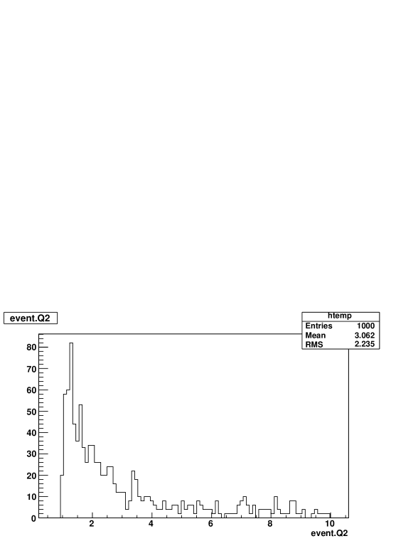
Figure 6: The resulting distribution of $Q^{2}$ from running the example program described in the text.

4.4 Runcard for look-up table generation

The following is showing an example runcard for the table generator, named “tableGeneratorRuncard.txt”:

⬇

//==============================================================

//

// Example Runcard for Sartre Table Generator.

//

// Comments start with a # or #

// Name and value are separated by a "=": name = value

// (alternatively ":" can be used as well)

//==============================================================

# Nucleus’ atomic number

A = 197

# Which moments of the amplitude to calculate:

# 0 <A> analytical, <A2> averaged over configurations (Default)

# 1 <A> only, analytical

# 2 <A2>, and <A> both averaged over configurations

modesToCalculate = 0

# Rootfile This is a prefix table type ("T", "L", "T2" or "L2"),

# as well as ".root" will be appended

rootfile = bintests

# Meson to generate (jpsi=443, phi=333, rho=113, DVCS=22)

vectorMesonId = 443

# Model, options are bSat, bNonSat, bCGC

dipoleModel = bSat

# Path for the b-dependence lookup table for bSat/bNonSat.

# Not used with bCGC.

bSatLookupPath = /usr/bin/sartre/bSatLookupTable/

numberOfConfigurations = 500

# Kinematic range, Q2 and t in Gev2, W in GeV

Q2min = 0.1

Q2max = 10.

Wmin = 60

Wmax = 110

tmin = -.5

tmax = -.0

# Number of bins in the tables:

Q2bins = 30

W2bins = 25

tbins = 40

# If a run fails, use the backup and continue:

# If in doubt use the tableInspector to make sure the rest

# of the runcard is as it should be.

useBackupFile = false

startingBinFromBackup=2

4.5 Generating look-up tables for amplitudes

The following is an example of a user program “tableGeneratorMain” for generating the first and second moments of the amplitude and store them in a look-up table:

⬇

#include <sstream>

#include <cstdlib>

#include <iostream>

#include "Amplitudes.h"

#include "TH1D.h"

#include "TFile.h"

#include "Constants.h"

#include "Table.h"

#include "TableGeneratorSettings.h"

#include "Enumerations.h"

int main(int argc, char *argv[]){

TH1::AddDirectory(false);

TableGeneratorSettings* settings = TableGeneratorSettings::instance();

//

// Check arguments

//

char* runcard;

if (argc != 4) {

cout<<"Usage: tableGeneratorMain runcard startBin endBin"<<endl;

return 1;

}

else{

runcard = argv[1];

settings->setStartBin(atoi(argv[2]));

settings->setEndBin(atoi(argv[3]));

}

settings->readSettingsFromFile(runcard);

settings->consolidateSettings();

int nBinQ2 = settings->Q2bins();

int nBinW2 = settings->W2bins();

int nBinT= settings->tbins();

double Q2min= settings->Q2min();

double Q2max= settings->Q2max();

double Wmin= settings->Wmin();

double Wmax= settings->Wmax();

double W2min=Wmin*Wmin;

double W2max=Wmax*Wmax;

double tmin= settings->tmin();

double tmax= settings->tmax();

unsigned int massA=settings->A();

int vmPDG = settings->vectorMesonId();

DipoleModelType model = settings->dipoleModel();

int startingBin=settings->startBin();

int endingBin=settings->endBin();

int modes=settings->modesToCalculate();

Table tableT;

Table tableL;

Table tableT2;

Table tableL2;

bool logQ2=true, logW2=false, logT=false, logC=true;

//set filenames for the tables:

string rootfile=settings->rootfile();

ostringstream filenameT, filenameL, filenameT2, filenameL2;

filenameT.str("");

filenameT<<rootfile<<"_bin"<<startingBin<<"_T.root";

filenameL.str("");

filenameL<<rootfile<<"_bin"<<startingBin<<"_L.root";

filenameT2.str("");

filenameT2<<rootfile<<"_bin"<<startingBin<<"_T2.root";

filenameL2.str("");

filenameL2<<rootfile<<"_bin"<<startingBin<<"_L2.root";

(void) tableT.create(nBinQ2, Q2min, Q2max,

nBinW2, W2min, W2max,

nBinT, tmin, tmax,

logQ2, logW2, logT, logC, // all bools

mean_A, transverse,

massA, vmPDG, model,

filenameT.str().c_str());

(void) tableL.create(nBinQ2, Q2min, Q2max,

nBinW2, W2min, W2max,

nBinT, tmin, tmax,

logQ2, logW2, logT, logC, // all bools

mean_A, longitudinal,

massA, vmPDG, model,

filenameL.str().c_str());

(void) tableT2.create(nBinQ2, Q2min, Q2max,

nBinW2, W2min, W2max,

nBinT, tmin, tmax,

logQ2, logW2, logT, logC, // all bools

mean_A2, transverse,

massA, vmPDG, model,

filenameT2.str().c_str());

(void) tableL2.create(nBinQ2, Q2min, Q2max,

nBinW2, W2min, W2max,

nBinT, tmin, tmax,

logQ2, logW2, logT, logC, // all bools

mean_A2, longitudinal,

massA, vmPDG, model,

filenameL2.str().c_str());

//Create and initialize the amplitudes calculator:

Amplitudes amps;

//Generate the the nucleon configurations:

amps.generateConfigurations();

// Print out settings:

cout<<"Tables will be generated for:"<<endl;

cout<<"Mode to calculate: "<<modes<<endl;

cout<<"Vector Meson Id: "<<vmPDG<<endl;

cout<<"Bins: "<<startingBin<<"-"<<endingBin<<endl;

cout<<"Q2 range: ["<<Q2min<<", "<<Q2max<<"], "<<nBinQ2

<<" bins."<<endl;

cout<<"W2 range: ["<<W2min<<", "<<W2max<<"], "<<nBinW2

<<" bins."<<endl;

cout<<" t range: ["<<tmin<<", "<<tmax<<"], "<<nBinT<<" bins."<<endl;

cout<<"Dipole Model: "<<model<<endl;

cout<<endl;

cout<<"Filling tables..."<<endl;

time_t tableFillStart = time(0);

for(int i=startingBin; i<endingBin; i++) {

double Q2, W2, t;

tableT.binCenter(i, Q2, W2, t);

//calculate contents and fill tables:

amps.calculate(t, Q2, W2);

double aT=amps.amplitudeT();

double aL=amps.amplitudeL();

if(massA>1){

tableT.fill(i, aT);

tableL.fill(i, aL);

}

if(modes!=1){

double aT2=amps.amplitudeT2();

double aL2=amps.amplitudeL2();

tableT2.fill(i, aT2);

tableL2.fill(i, aL2);

}

}

cout<<"CPU Time/Entry: " << double(time(0)-tableFillStart)/endingBin

<<" s/entry."<<endl;

cout<<"Total time: "<<double(time(0)-tableFillStart)/60./60.

<<" h"<<endl;

if(massA>1){

tableT.write();

tableL.write();

}

if(modes!=1){

tableT2.write();

tableL2.write();

}

return 0;

}

5 Acknowledgements

The authors would like to thank Henri Kowalski, Tuomas Lappi, Thomas Burton and Raju Venugopalan for their input and help, and the Open Science Grid consortium for providing resources and support. This work was supported by the U.S. Department of Energy under Grant No. DE-AC02-98CH10886.

Appendix A The tables

A table in Sartre is internally stored in a three-dimensional ROOT histogram. The Table class encapsulates the histogram and provides many methods to easily store and access information. The tables are stored in ROOT files. To create a table, one calls:

Table::create(int nbinsQ2, double Q2min, double Q2max,
              int nbinsW2, double W2min, double W2max,
              int nbinsT, double tmin, double tmax,
              bool logQ2, bool logW2, bool logt, bool logContent,
              AmplitudeMoment mom, GammaPolarization pol,
              unsigned int A, int vm,
              DipoleModelType model, const char* filename)

where the first nine arguments define the limits in $Q^{2}$, $W^{2}$, and $t$, as well as the granularity of the table, i.e. the number of bins in each directions. The booleans, e.g. logQ2, indicate whether the binning is linear in $Q^{2}$ or in $\log Q^{2}$, logContent indicates whether the content is stored linearly or logarithmically. Also, one needs to provide information on whether one calculates the first or second moment of the amplitude, with which polarization of the virtual photon (see table 1), with which atomic number of the nucleus and which dipole model is used. Table::create also requires a file-name to which the table can be saved. There is also a mechanism for making back-ups for tables during the generation process.

All of this information (except file name) is coded into a 64bit word that is also used as the histogram title. It is to be interpreted as an uitn64_t with the bits set as follow:

bit 0: content type: 0 for $\left<\mathcal{A}\right>$, 1 for $\left<|\mathcal{A}|^{2}\right>$
bit 1: polarization: $L$ for 0, $T$ for 1
bit 2: $t$ encoding: 0 for $|t|$, 1 for $\log(|t|)$
bit 3: $W^{2}$ encoding: 0 for linear, 1 for logarithmic
bit 4: $Q^{2}$ encoding: 0 for linear, 1 for logarithmic
bit 5-7: dipole model type
bit 8-15: mass number A
bit 16-31: vector meson ID (PDG)
bit 32: content encoding: 0 in linear, 1 in logarithmic
bit 33: content type is $\lambda$ (bit $0=0$ in this case)
bit 33-63: not used

When reading a value from a table, e.g. to calculate a cross section in a phase-space point, one calls the function Table::get(double Q2, double W2, double t). In general, the values of $Q^{2}$, $W^{2}$, and $t$ asked for will not correspond with a bin-center in the histogram, so the stored points are used to interpolate to the value asked for. For this interpolation to be accurate, the histogram has to be fine enough in its binning.

For the corrections, described in eq. (16) and eq. (17), special tables are generated containing $\lambda$ as described in eq. (16). If the range of the $\lambda$-table is smaller than for the amplitude table, the fall-back option is to calculate the derivative using the proton amplitude tables. If the range of these tables also are too small corrections will not be applied.

References

- [1] K. J. Golec-Biernat and M. Wusthoff, Phys. Rev. D 59, 014017 (1998).
- [2] K. J. Golec-Biernat and M. Wusthoff, Phys. Rev. D 60, 114023 (1999).
- [3] J. Bartels, K. J. Golec-Biernat and H. Kowalski, Phys. Rev. D 66, 014001 (2002).
- [4] T. Toll, T. Ullrich [arXiv:1211.3048 [hep-ph]].
- [5] A. Deshpande, Z. -E. Meziani, J. -W. Qiu, R. McKeown, S. Vigdor, E. C. Aschenauer, W. Brooks and M. Diehl et al., arXiv:1212.1701 [nucl-ex].
- [6] T. Sjostrand, P. Eden, C. Friberg, L. Lonnblad, G. Miu, S. Mrenna and E. Norrbin, Comput. Phys. Commun. 135, 238 (2001) [arXiv:hep-ph/0010017].
- [7] M. Bahr et al., Eur. Phys. J. C 58, 639 (2008) [arXiv:0803.0883 [hep-ph]].
- [8] G. Ingelman, A. Edin and J. Rathsman, Comput. Phys. Commun. 101, 108 (1997) [arXiv:hep-ph/9605286].
- [9] L. Mankiewicz, A. Schafer and M. Veltri, Comput. Phys. Commun. 71, 305 (1992).
- [10] H. Jung, Comput. Phys. Commun. 86, 147 (1995).
- [11] L. Lonnblad, Comput. Phys. Commun. 71, 15 (1992).
- [12] H. Jung, Comput. Phys. Commun. 143, 100 (2002) [arXiv:hep-ph/0109102].
- [13] T. Gleisberg, S. Hoeche, F. Krauss, M. Schonherr, S. Schumann, F. Siegert and J. Winter, JHEP 0902, 007 (2009) [arXiv:0811.4622 [hep-ph]].
- [14] S. Roesler, R. Engel and J. Ranft, arXiv:hep-ph/0012252.
- [15] Jean-Paul Sartre 1946, Existentialism Is a Humanism. Translated by Philip Mairet.
- [16] H. Kowalski and D. Teaney, Phys. Rev. D 68, 114005 (2003).
- [17] B. Z. Kopeliovich, J. Nemchik, A. Schafer and A. V. Tarasov, Phys. Rev. C 65, 035201 (2002).
- [18] H. Kowalski, L. Motyka, G. Watt, Phys. Rev. D74, 074016 (2006).
- [19] S. R. Klein and J. Nystrand, Phys. Rev. Lett. 84, 2330 (2000).
- [20] H. Kowalski, T. Lappi, C. Marquet and R. Venugopalan, Phys. Rev. C 78, 045201 (2008).
- [21] R. J. Charity, ”Advanced Workshop on Model Codes for Spallation Reactions” (Trieste, Italy: IAEA) p 139 report INDC(NDC)-0530.
- [22] R. Brun and F. Rademakers, Nucl. Instrum. Meth. A 389, 81 (1997).
- [23] M. Galassi et al, GNU Scientific Library Reference Manual (3rd Ed.), ISBN 0954612078.
- [24] T. Hahn, Nucl. Instrum. Meth. A 559, 273 (2006) [hep-ph/0509016].
- [25] BOOST C++ library, http://www.boost.org/
- [26] C. W. De Jager, H. De Vries and C. De Vries, Atom. Data Nucl. Data Tabl. 14, 479 (1974).