Optimising Spectroscopic and Photometric Galaxy Surveys: Efficient Target Selection and Survey Strategy

Abstract

The next generation of spectroscopic surveys will have a wealth of photometric data available for use in target selection. Selecting the best targets is likely to be one of the most important hurdles in making these spectroscopic campaigns as successful as possible Our ability to measure dark energy depends strongly o the types of targets that we are able to select with a given photometric data set We show in this paper that we will be able to successfully select the targets needed for the next generation of spectroscopic surveys. We also investigate the details of this selection, including optimisation of instrument design and survey strategy in orde to measure dark energy We use color-color selection as well as neural networks to select the best possible emission line galaxies and luminous red galaxies for a cosmological survey. Using the Fisher matrix formalism we forecast the efficiency each target selection scenarios. We show how the dark energy figures of merit change in each target selection regime as a function of target type, survey time survey density and other survey parameters We outline the optimal target selection scenarios and survey strategy choice which will be available to the next generation of spectroscopic surveys

accepted to MNRAS dec 2013

1 Introduction

One of the goals of the next decade of cosmological surveys is to understand what causes the accelerated expansion of the Universe. This involves understanding the nature and behaviour of dark energy and dark matter. To begin to answer these questions, several photometric and spectroscopic surveys are being planned to start over the next 10 years. The Dark Energy Survey, hereafter DES, is the first of a new generation of photometric surveys that focuses on dark matter and dark energy studies. DES will start observing on the fall of 2013. DES will be followed by the Euclid experiment whose launch is scheduled for 2020 and the Large Synoptic Survey Telescope (LSST) on a similar timescale. On the same timescale as DES, HypersuprimeCam will map around 2000 square degrees in the sky, to greater depth than DES, in similar optical bands.

In terms of spectroscopic surveys, the Sloan Digital Sky Survey (SDSS) and BOSS surveys have mapped, or are currently mapping, the large scale structure of our Universe. They have targeted Luminous Red Galaxies (LRGs) out to redshift $z\approx 0.7$. The next generation of surveys will survey deeper than SDSS and BOSS by also using the Emission Line Galaxies (ELGs). This strategy has already been used by the WiggleZ Dark Energy survey Drinkwater et al. (2010) which targetted ELGs in looking at their NUV flux with the Galaxy Evolution Explorer (GALEX) satellite (Martin et al. 2005). GALEX NUV has a detection limit of 22.8. This paper aims to investigate deeper targetting strategy in order to go up to i$\approx$23.5. We thus study observational strategies for future spectroscopic surveys using current and future photometric surveys such as DES, LSST, Euclid.

Abdalla et al. (2008) showed that we can predict emission lines from broadband photometry using Neural network (NN) algorithms. In general it would be possible to use such techniques in target selection studies. We present a target selection approach based on the use of NN and broad-band photometry. Despite the complex selection function that this strategy represents, it can efficiently recover a galaxy’s redshift based on spectra We assess in this paper to what extent several networks can help improve target selectio and survey strategy

We analyse different strategies of target selection using color-color or more complex techniques such as a neural network target selection. We use different surveys for the photometry depending on the type of galaxies we want to select: ELGs at high redshift; LRGs at lower redshift. Section 2 describes the goals of future cosmological spectroscopic surveys and photometric surveys that can be used for target selection. We make our comparisons using mock catalogues that we describe in section 3. In Section 4 we outline the neural network target selection we use in this work. In sections 5 and 6 we outline our possible strategies for selection of LRGs and ELGs. Finally, we investigate how the target selection affects the survey strategy and the Figures of Merit (FoM) for dark energy in section 7.

2 Current spectroscopic surveys and future plans

2.1 Cosmological spectroscopic surveys

In order to meet the goals of the current and next generation of cosmological spectroscopi surveys and improve on our knowledge of dark energy, we nee to acquire on the order of a thousend or more galaxy redshift per square degree up to redshifts of order unity and we need to do this ove several thousands of square degrees. In this sectio we outline the possible sources of photometry that can be used to defin an efficient target selection strategy Several proposals have been developped such a DESpec (Abdalla et al. 2012) which is a spectroscopic survey over the DE footprint and BigBOSS (Schlegel et al. 2011) Both of the above projects have recently been merged into one umbrella project i.e. the Mid Scale Dark Energy Spectrocopic Instrument (MS-DESI)

Concerning DE experiments, the main interests of spectroscopic surveys is to help at calibrating systematic errors of photometric surveys such as Intrinsic Alignements and photometric redshift uncertainty that affect the WL, cluster counts and BAO probes. The other main interest is the precise information they provide in the radial direction. The large scale photometric surveys will use photometric redshift to set the galaxy distances using several photometric bands. The number and width of the bands is not adapted to high accuracy photometric redshift such as the PAU survey (Gaztañaga et al. 2012). Spectroscopic redshifts allow us to access radial modes at high frequency due to the high precision redshift information. They are then used to study redshift space distortions (RSDs) which will help tightening DE constraints when combined with the other DE probes such as shown in the SDSS results of Reid et al. (2012) or the WiggleZ results of Blake et al. (2012).

BigBOSS was planning to study the Baryon Accoustic Oscillation using ELGs up to z$\sim$1.7 and quasars up to z$\sim$3 at the NOAO 4‑meter Mayall Telescope on Kitt Peak in Arizona. It will survey 14,000 square degrees on the northern hemisphere and 10,000 square degrees on the southern hemisphere. The DESpec survey was planning to cover at least the DES footprint of 5000 square degrees. The final strategy for DESI is not yet set on stone. The area may extend up to 15,000 square degrees by also using LSST photometry for spectroscopic target selection. The DES and LSST photometry (together with VISTA JHK photometry) yields not only fluxes and photometric redshifts but also galaxy image shapes and surface brightnesses. All of this information can be exploited in various ways to select a sample of galaxies that satisfy the joint requirements of large redshift range, adequate volume sampling, and control over any bias introduced due to sample selection or redshift failures. In practice, we expect to use galaxy flux, color (and photo-z), and surface-brightness to sculpt the redshift distribution of the survey.

In this paper, our spectroscopic targetting strategy is to target a mix of emission-line galaxies (ELGs)—which predominate at high redshift and which yield efficient redshift estimates to z$\sim$1.7 based on their prominent emission lines —and luminous red galaxies (LRGs), with brighter continuum spectra, which offer high redshift success rates at lower redshifts, up to z$\sim$1. The target selection will ultimately be chosen to optimize the science yield; at this stage, we present some examples of survey selection to demonstrate its feasibility.

2.2 Current and future surveys useful to target selection

The photometry from current and future surveys will be useful to the selection of targets in DESI and other spectroscopic surveys such as eBOSS , SUMIRE, 4MOST (de Jong et al. 2012). In order to test the different target selection strategies and their impact on DE science outputs, we simulated different surveys with mock catalogues that we describe in section 3.

We aim at covering a wide area on the sky with a wavelength range that will allow the study of galaxy population and large scale structure at high redshift. Past and current spectroscopic surveys are either large and relatively shallow such as BOSS and SDSS, which cover several thousands of square degrees up to z $\approx$0.7, or deep on a small field such as Wigglez, VVDS, zCOSMOS, and VIPERS. These deep surveys can go up to z$\approx$6 but rarely cover more than several hundreds of square degrees. We need to define a target selection based on large photometric surveys. To compare the impact of photometric depth in the target selection, we simulate the photometry of optical surveys such as the DES, the Palormar Transient Factory (PTF), and PanSTARRS (PS1). Between them these surveys represent the range of area/depth options currently under consideration. The photometry from these surveys allows for different target selections that form the basis of this paper.

To complement optical surveys, the DES footprint overlaps with the VISTA/VHS. This produces better photometric redshifts as studied in Banerji et al. (2008) and will help the target selection for galaxies at $z>1$. In the next sections, we will consider a target selection based on deep photometry using the DES+VISTA surveys.

We also simulated WISE photometry. Galaxies show a 1.6$\mu$ m bump restframe that will be used in the target selection of higher redshift galaxies with the w1 photometry. We detail the different target selection in the next sections depending on the type of galaxies we are targetting such as LRGs in section 5 and ELGs in section 6.

To give a quick overview of these surveys:

• DES will cover 5000 deg² in 5 photometric bands covering 0.4 to 1 $\mu$m to a depth of i-band 24 mag AB at 5$\sigma$ in the aim of studying the large scale structures from the cosmic shear and BAO signal, the supernovae and galaxy clusters. The first observations will start in november 2012 and last for 5 years. DES fields are located in the southern hemisphere and are visible during 4 months at the end of the year.

• PTF is an ongoing transient survey targeting 8000 deg²/yr in the 2 photometric bands R and g’ to study mainly supernovae, binaries and transiting planets. The survey will last 5 years and will do a full sky area.

• panSTARRS is an ongoing survey that will cover a full sky area in 5 photometric bands covering the same wavelength range as the DES survey. panSTARRS strategy is divided in 4 stages. Each stage will complete a full sky and increase the deth from the precedent stage. In this paper, we simulate the photometry of stage 1.

• VISTA/VHS will cover 19000 deg² in the southern hemisphere to study the Milky Way, discover nearby stars and low mass stars, study Dark Energy out to z$\approx$1 and high redshift quasars using NIR photometry.

• WISE will survey the entire sky in mid-IR photometry to study asteroids of our solar systems, nearby stars, the Milky Way, and AGN.

We give the depth at 5$\sigma$ of the different photometric bands of the surveys that we describe in this section in Table LABEL:tab:survey_depth. We concentrate on the bands that we are planning to use in the target selection. We show the bands wavelength coverage and 5 $\sigma$ depth for extended objects in Figure 1.

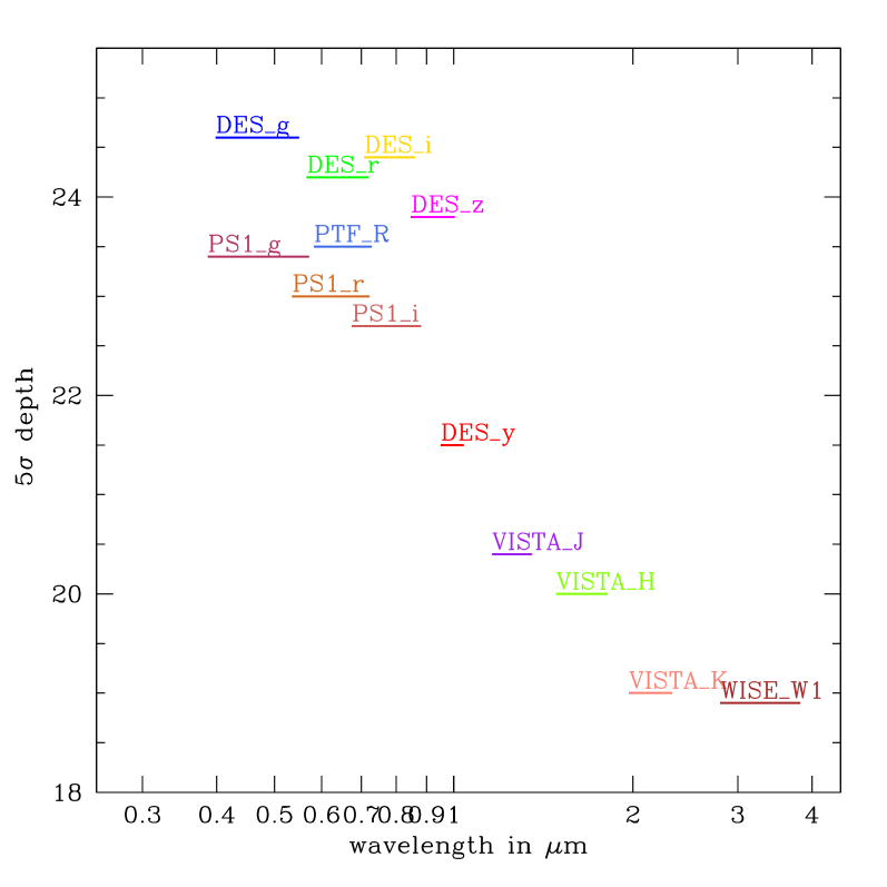
Figure 1: Band width in $\mu$m and 5$\sigma$ depth of extended sources for the DES survey, PanSTARRS 1 year survey, PTF R band and VISTA JHK bands.

Table 1: Photometry of surveys used in for the targets selection. The table shows the depth of extended sources at 5$\sigma$.

Survey	Band	AB mag(5$\sigma$)
DES	$g$	24.6
DES	$r$	24.2
DES	$i$	24.4
DES	$z$	23.8
DES	$y$	21.5
VISTA	$J$	20.4
VISTA	$H$	20.0
VISTA	$K$	19.0
PS1	$g$	23.4
PS1	$r$	23.0
PS1	$i$	22.7
PTF	$R$	23.5
WISE	3.6um	18.9

3 Spectro-photometric simulations

3.1 The COSMOS Mock Catalogue

To quantify the yield of a particular spectroscopic scheme, we use the COSMOS Mock Catalogue (CMC) Jouvel et al. (2009); Zoubian & Kneib (2013). The CMC is built from the COSMOS photometric-redshift catalogue Capak et al. (2008); Ilbert et al. (2009). We use the CMC to predict the target number density and to compute the spectroscopic instrument sensitivities. The COSMOS photometric-redshift catalog (Ilbert et al. 2009) was computed with 30 bands from GALEX for the UV bands, Subaru for the optical, CFHT, UKIRT and Spitzer for the NIR bands over 2 deg². The CMC is restricted to the area fully covered by HST/ACS imaging, 1.24 deg2 after removal of masked areas. There are a total of 538,000 simulated galaxies for $i<26.5$ leading to a density of roughly 120 gal/arcmin². The CMC includes AGN and star. COSMOS have high quality photo-z with an excellent accuracy and low catastrophic redshift rates from a careful calibration with the spectroscopic samples zCOSMOS and MIPS. To derive properties used in the simulations from each observed COSMOS galaxy, a photo-z and a best-fit template spectrum (including possible additional extinction) are associated with each galaxy of the COSMOS catalog. We first integrate the best-fit template through the instrument filter transmission curves to produce simulated magnitudes in the instrument filter set. We then apply random errors to the simulated magnitudes based on a simple magnitude-error relation in each filter. The simulated mix of galaxy populations is then, by construction, representative of a real galaxy survey, and additional quantities measured in COSMOS (such as galaxy size, UV luminosity, morphology, stellar masses, correlation in position) can be easily propagated to the simulated catalog. The COSMOS mock catalog is limited to the range of magnitude where the COSMOS imaging is complete ($i_{AB}\approx 26.2$ for a 5 $\sigma$ detection (Capak et al. 2007, 2008). We associate emission-line fluxes for each galaxy of the CMC. We model the emission-line fluxes of each galaxy using the Kennicutt (1998) calibration which links the star-formation rate (SFR) from the dust-corrected UV rest-frame luminosity already measured for each COSMOS galaxy. The SFR is then translated to an [OII] emission-line flux using another calibration from Kennicutt (1998). We model the Balmer lines (Ly, Hb, Hd, Hg, Ha), the oxygen lines (OII, OIIIa, OIIIb), the nitrogen line (NII) and the sulfur lines (SIIa, SIIb) from emission line ratios McCall et al. (1985); Moustakas et al. (2006); Mouhcine et al. (2005); Kennicutt (1998) and zCOSMOS spectroscopic data. The relation found between the [OII] fluxes and the UV luminosity is in good agreement with the VVDS data and still do not vary for different galaxy populations as shown in Jouvel et al. (2009). Jouvel et al. (2009) validates the CMC and show that it reproduces the counts and color distributions from the optical to NIR bands in comparing to the GOODS (Giavalisco et al. 2004) and UDF (Coe et al. 2006) surveys. The CMC also provides an excellent match to the redshift-magnitude and redshift-color distributions for I$<$24 galaxies in the VVDS spectroscopic redshift survey (Le Fèvre et al. 2005).

3.2 Sensitivities and signal-to-noise for spectroscopic surveys

We choose here one spectrograph configuration which corresponds to a DESpec-like survey but stress that the optimisation procedure in further section remain applicable to any target selection study. We simulate the spectroscopic instrument throughput, sensitivities, exposure time, and success rate using the simulated galaxy spectra produced by the COSMOS Mock Catalogue (CMC, Jouvel et al. (2009)) and from the DES galaxy catalogue simulations (R. Wechsler & M. Busha). Both model galaxy physics such as emission lines, dust extinction, at redshift ranges and magnitudes appropriate to our spectroscopic survey.

The DES catalog simulations provide galaxy spectra based on the template models generated by the Kcorrect package Blanton & Roweis (2007), while as just described the CMC provides spectra based on the COSMOS data, providing in particular detailed distributions of line fluxes for emission-line galaxies. We then fold in the various contributions to the overall system throughput, specifically the transmission vs. wavelength for the atmosphere, the telescope and spectrograph optics, and the fibers, plus the quantum efficiency of the CCD detectors.

In this study we have assumed a 50% throughput efficiency for the spectrograph plus fibers and used the size distribution of our galaxies to obtain the correct amount of light gathered. We have used standard cross correlation techniques to obtain the spectroscopic efficiency of our instrument once noise has been added to the simulations. We have assumed 2-arcsec-diameter fibers and a resolution of $R=3500$ at 900nm for these calculations. For the detailed calculations for the sensititvies of the fidutial spectrograph we refere the reader to (Abdalla et al. 2012).

4 Target selection: NN and color-color

Several surveys used color-color selection to sculpt the redshift distribution in order to study specific redshift ranges of the galaxy population such as DEEP2, VIPERS. DEEP2 select galaxies between 0.75$<$z$<$1.4 with photometry in BRI bands, VIPERS select galaxies from 0.5$<$z$<$1.4 with photometry u⁢gri bands. The resulting surveys show that it is possible to select galaxy targets based on color-color selections which work well to realise a broad redshift selection.

In the future, during the next five years, the DES and VISTA surveys in the south, and in the next ten years LSST and Euclid over the whole sky, will provide rich photometric data on wide wavelength ranges from optical to NIR. In this paper, we present a way of utilising DES and VISTA broadband photometry in order to do an optimized galaxy target selection. We show a new technique based on NN fed with the photometry from surveys such as those mentioned above. A NN technique is similar to a multi-dimensional color-color selection. It assumes multi-color informations for 4 or more bands. The network captures emission line features from ELG colors using the extra color information provided by the multi-band surveys.

Throughough the paper, we use ANNz (Collister & Lahav 2004). Abdalla et al. (2008) shows that one can predict emission line strength from galaxy colors. As we briefly explained in section 3, the CMC simulation predicts emission lines fluxes and include them in the galaxy magnitudes derived. Using the CMC multi-color information from the DES+VHS surveys, we teach the neural network to recognise ELGs using a representative training sample of 10000 galaxies.

Figure 2 is a schematic representation of the NN target selection. The left bubble represents a training sample for which the blue dots symbolise strong emission line galaxies that we want to target, and the black dots other types of galaxies. To realise the selection, we assume a telescope model using the sensitivity curves described in section 3.2. We train the NN using a target/not-a-target selection and test it on a sample equally representative of the training and validation sample. The NN outputs a number which can be associated with a probability of the galaxy being of the type you trained the NN to recognise. We then trade off between galaxy number density and purity of the sample in choosing a probability value that defines whether the galaxy is a target.

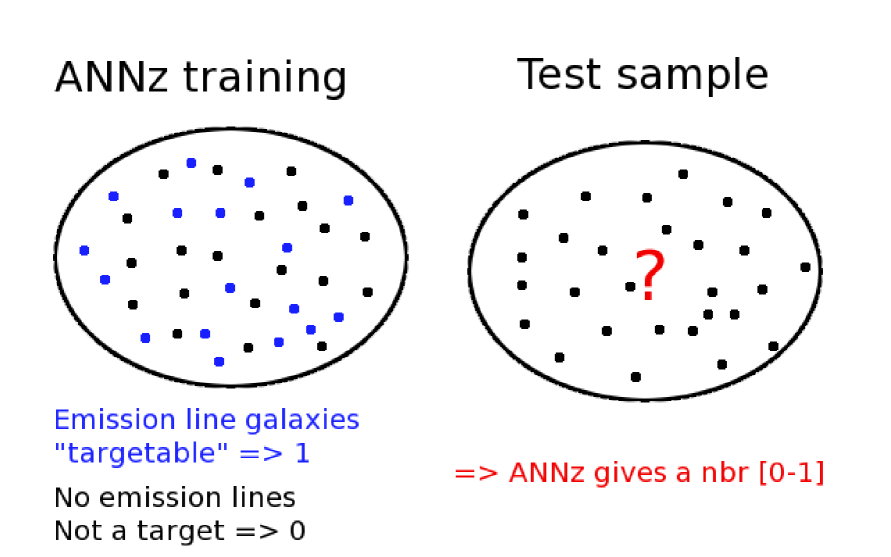
Figure 2: Schematic representation of the targetting strategy using Neural Network. The blue dotted points correspond to the galaxies with strong emission lines for which we will be able to measure a redshift using our spectroscopic sensitivities. The black dot correspond to the galaxies with weak or none emission lines galaxies.

We use the NN target selection to select ELGs and LRGs following the procedure we describe in this section. We also realise 2 more traditional color-color selections to compare results. We detail below the 3 target selection methods we study in this paper.

• Shallow color-color target selection: photometry from panSTARRS, PTF and WISE

• Deep color-color target selection: photometry from DES+VHS

• NN target selection: photometry from DES+VHS

We further compare the different targetting strategies for LRGs and ELGs in section 5 and section 6.

5 Targetting strategy for LRGs

5.1 Strategy and plans for LRGs

In order to measure the BAO signal to redshift z$\approx$1 we need of order $\approx$300 luminous red galaxies per sq. deg. Results from SDSS and BOSS indicate that LRG targets in this redshift range should have a high rate of redshift success. For galaxy clustering measurements, LRGs are convenient because they occupy dense regions and are thus strongly biased relative to the dark matter, b$\approx$2 as quoted in Dawson et al. (2013). With our simulations we have estimated the completeness rate for objects in the CMC catalogue. We also plot in Figure 3 a preliminary example of a redshift completeness for LRGs, showing the magnitude, as a function of redshift, where the redshift success rate is expected to be 90%, based on the above simulations and assumptions. Also shown on the plot is the apparent magnitude vs. redshift relation for an LRG, taken to be a 3L* galaxy (Eisenstein et al. 2001), showing that we will be 90% complete for LRG redshift measurement out to z = 1.3 in a 30 minute exposure. Given that the redshifts of these galaxies are attainable by our spectroscopic instrument out to redshifts just higher than one with a 30 min exposure time we aim to obtain a target selection from the photometric data.

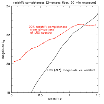
Figure 3: The red points and curve indicate the $i_{AB}$ magnitude vs. redshift where the redshift success rate for an LRG spectrum is 90%, based on our spectroscopic simulations. Also plotted in black is the magnitude vs. redshift relation for an LRG, taken as a 3L* galaxy (Eisenstein et al. 2001), showing that we will be 90% successful for LRG redshift measurements out to $z=1.3$ in a 30 minute exposure.

5.2 LRGs target selection using deep optical-NIR photometry

Using DES+VHS imaging, we can target the LRGs with z-mag less than the depth of DES and yielding a relative flat redshift distribution over the range 0.5$<$z$<$1. We use selection cuts in r-z vs. z-H color space in addition to a magnitude selection of $z_{DES}$. We show the colour diagrams in Figure 4. These cuts supply more than the needed density of LRG targets, so they can be randomly sampled. This r-z cut

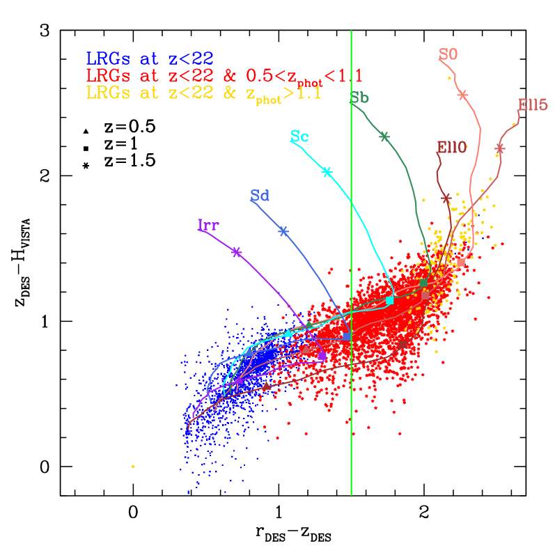
Figure 4: LRGs target selection using DES+VHS photometry. Example of the targeting efficiency of color-color cuts for galaxies at magnitude z$<$22, in blue for a redshift z$<$0.5, green for 0.5$<$z$<$1.1, and gold for z$>$1.1.

5.3 Target selection using shallow optical-IR photometry

As a comparison, we use the CMC simulation of the PTF, panSTARRS and WISE photometry and reproduce the target selection of the BigBOSS surveys. Figure 5 shows R-i from the PTF and panSTARRS surveys versus R-W1 color from the PTF and WISE surveys. The LRGs selection consist in targetting all the galaxies that are above the black line. In black we show all galaxies for which W1$<$18.9. In magenta and blue we show galaxies at $z>0.55$ for which respectively W1$<$18.9 and W1$<$19.9. The PTF+WISE selection is aiming to select bright LRGs based on the 1.6um bump for galaxies at $z>0.5$. This selection allow to select a sample of galaxies whose mean redshift will be around $z\approx 1$.

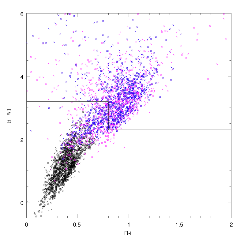
Figure 5: LRGs target selection using PTF+WISE photometry. This figure shows R-i as a function of W1-R colors in black for all galaxies for which W1$<$18.9. We also show galaxies at z$>$0.55 for which W1$<$18.9 in magenta and W1$<$19.9 in blue.

5.4 LRGs target selection using NN

We use DES and VHS photometry and train the NN to select elliptical galaxies at i brighter than 23 AB magnitude without redshift restriction. The CMC is built from the best-fit template and photometric redshift of the COSMOS survey. Using the COSMOS galaxy types of the CMC we are able to select elliptical galaxies from DES+VHS colors using NN such as explained in section 4. Figure 6 shows the cumulative distribution of ANNz probability distribution values for galaxies brighter than i $\approx$ 23, 23.5, and 24 in respectively small-dashed, dotted and solid lines. The blue lines are the cumulative number of LRGs selected by the NN while the black lines are other types of galaxies. The green lines give the number density of galaxies selected using the color-color cut with DES+VHS photometry in solid lines and the density of LRGs inside the color-color cut in long-dashed lines. In a same way, the cyan lines represent the number density of galaxies and LRGs selected using the PTF+WISE photometry cut.

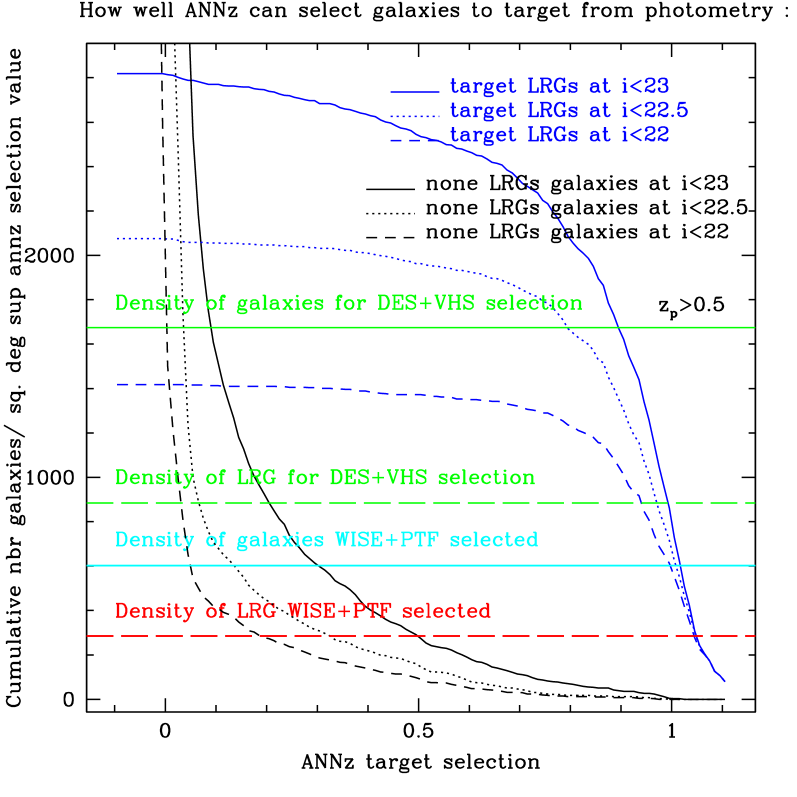
Figure 6: Cumulative number of galaxies as fct of ANNz target selection for LRG. Overplotted the number density for the color-color selections

5.5 Redshift distribution of color and NN selection for LRGs

Here we compare the redshift distribution of the different targetting strategies. Figure 7 shows the redshift distribution of the 2 color-color section PTF+WISE, DES+VHS and the NN selection in respectively black solid, long dashed-dotted green and small dashed-dotted blue lines. For the NN selection, we add a photometric redshift cut at $z_{p}>0.5$ since we are interested mostly in the high-redshift LRGs at $0.5<z<1$ as explained in the survey definition section 2.

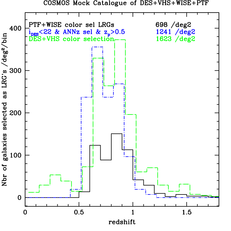
Figure 7: Redshift distribution for the color-color selection PTF+WISE and DES+VHS and the NN selection in respectively black solid, long dashed-dotted green and small dashed-dotted blue lines. We realise a cut in the NN selection at $i_{DES}<22$ with a photometric redshift at $z_{p}>0.5$.

The DES+VHS color-color selection yields the highest number of LRGs with a density of 1623gal/deg² compared to 1241gal/deg² for the NN selection and 698gal/deg² for the PTF+WISE selection. However the color-color targetting strategy has a broader range of galaxy types as you can see in Figure 8. Figure 8 shows the distribution of galaxy types for each of the targetting strategy: color-color using DES+VHS in green long dashed-dotted lines, color-color using PTF+WISE in black solid line, the NN and photometric redshift selection in blue small dashed-dotted lines at $i_{DES}<22$ and in red dashed lines for $i_{DES}<22.5$.

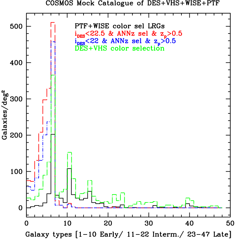
Figure 8: Histogram of types for the color-color PTF+WISE and DES+VHS and NN selection strategy in respectively black solid, long dashed-dotted green and small dashed-dotted blue lines. We realise a cut in the NN selection at $i_{DES}<22$ with a photometric redshift at $z_{p}>0.5$.

The types corresponds to the library templates used to derive the photometric redshift of the COSMOS survey. There is 8 ellipticals, 11 spirals and 12 starbursts from Bruzual & Charlot (2003) and Polletta et al. (2007) calibrated using the zCOSMOS and MIPS spectroscopic redshift surveys as explained in section 3. In this figure, the early type galaxies ranges from 1 to 10, followed by intermediate types from 11 to 22 and late types from 23 to 31. This figure shows that both color-color selection targets some intermediate and late types galaxies in their LRGs sample. The LRG targetting strategy relies on a redshift measurement based on the spectrum of the continuum. The intermediate and late types are less reliably determined from their continuum. This will likely lower the efficiency of the target selection. The PTF+WISE CC selection is shallower and have less contamination from the intermediate and late types. However in proportion, it is as affected as the DES+VHS CC selection. The NN selection works well at selecting the early-types galaxies from DES+VHS photometry and is not contaminated by intermediate and late types. The spectroscopic success rate will be higher in a NN selection than a CC selection. However, an NN+photoz selection is more complexe than a CC selection in terms of selection function. For clustering and galaxy evolution studies, you need to determine the completness of the galaxy sample. A NN+photoz selection will give more work on the understanding of the selection function.

5.6 Spectroscopic success rates of LRG target selection

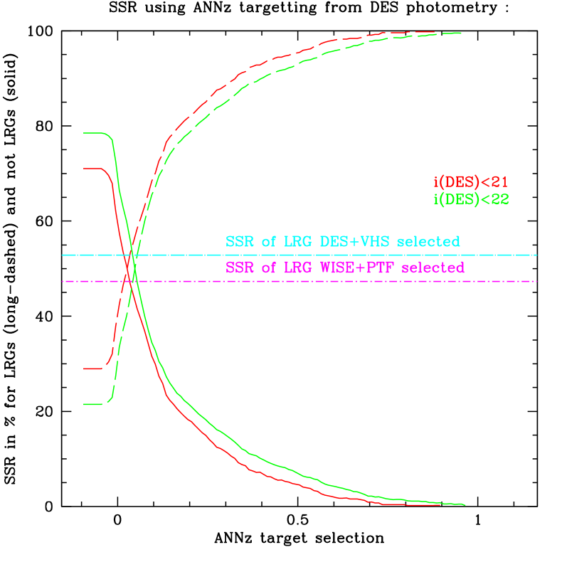
Figure 9: Spectroscopic Success Rate as a function of ANN selection values for the LRGs selected using DES+VHS photometry in long-dashed lines and for other types of galaxies in solid lines. The red and green lines select galaxies at respectively i brighter than 21 and 22. The long-dashed and small-dashed dotted lines are respectively the success rate of DES+VHS and PTF+WISE LRG color selection.

Figure 9 show the Spectroscopic Success Rate of the LRGs selection with ANNz in long-dashed lines at i brighter than 21 and 22 in respectively red and green lines. The other types of galaxies are shown in solid lines. A selection cut at 0.8 gives very high success rate with a NN selection. For i brighter than 21, there is no contamination by other types of galaxies and a very small percentage for i brighter than 22. As a comparison, we show the PTF+WISE and DES+VHS color selection in respectively small-dashed dotted magenta line and long-dashed dotted cyan line. Both color selections show similar success rates with respectively 48% and 53% for WISE+PTF and DES+VHS color selection of LRGs. Color selections allow a secure redshift measurement for about half of the galaxies targetted while the NN selection allows close to 98% redshift measurement. However, this study relies on several strong assumptions such as: 1. a perfect knowledge of galaxy populations 2. a non-biased photometry in the photon noise regime 3. a representative training sample. In a real survey, to perform this strategy, a few nights of spectroscopic data would be needed to train the NN response to this selection.

Figure 7 show that the NN selection reaches a number of galaxies close to the one reached using a color selection with the same photometry, DES+VHS in this figure. The NN gives a success rate close to 100%. However, we know that all the assumptions we made are unrealistic which will lower down the success rate of the NN and possibly the color selection as well. We will need to test both methods on more developped simulations of the instrument and on real data for a definite validation.

6 Targetting stragety for ELGs

In this section, we describe simulations to investigate selection criteria for a survey targeting emission-line galaxies at redshifts higher than accessible with luminous red galaxies for BAO and RSD studies. Using the CMC (Jouvel et al. 2009), we assume that the survey would reach the line sensitivities described earlier, namely a signal-to-noise ratio of around 5 for fluxes larger than 3e-17 erg/s/cm2 from wavelengths 600 to 1000 nm. This is reached for a 30 min exposure, which we take as the baseline.

We compare color target selection and NN selection for ELGs at $z>1$ in the same way we did in section 5.

6.1 Target selection using color cuts in the optical

DEEP2, VIPERS, Wigglez and other surveys used color selection in order to select emission line galaxies at some redshit ranges. The BigBOSS survey is planning to use PTF and panSTARRS photometry to realise the target selection. In this section, we reproduce the PTF-panSTARRS target selection using mock photometry of these surveys simulated using the CMC, see section 3.

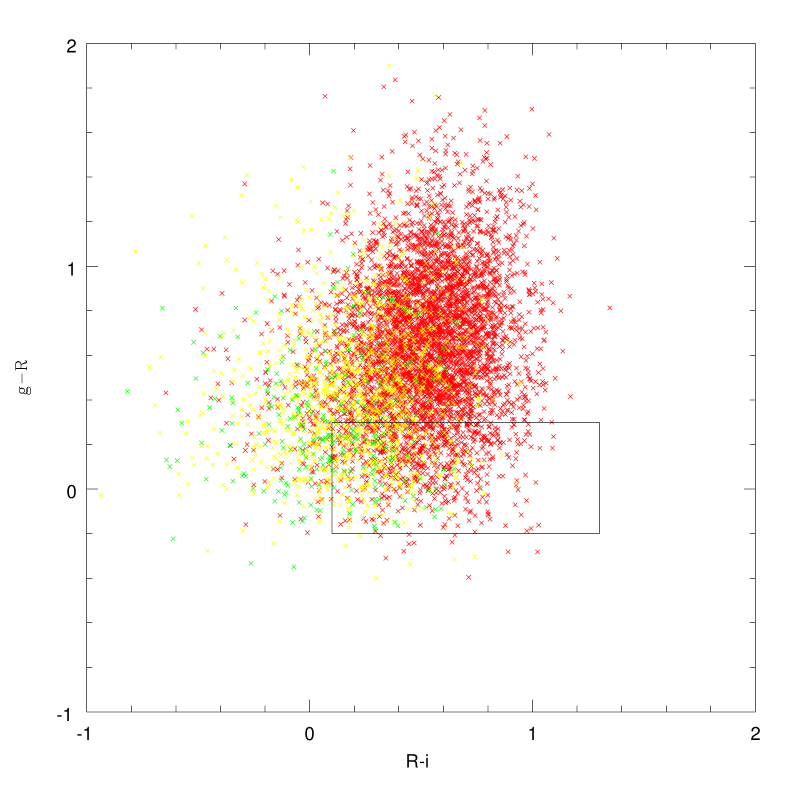
Figure 10: Color-color selection of ELG galaxies. The x-axis shows R-i of panSTARRS i band and PTF R band as a function of g-R of panSTARRS g band and PTF R band. The black box represent the color-color cut we apply to selec bright ELG galaxies at 0.7$<$z$<$2.

Figure 10 show R-i of panSTARRS i and PTF R band as a function of g-R of panSTARRS g and PTF R band. The black box represents the color cuts we apply to select bright ELG galaxies at 0.7$<$z$<$1.7. The green, yellow, and red points are galaxies at respectively 0.7$<$z$<$1.2, 1.2$<$z$<$1.6, and 1.6$<$z$<$2.

6.2 Target selection using NN techniques

We can use photometric redshifts to select for high-redshift galaxies. Figure 11 shows the redshift distribution of emission-line galaxies that our spectroscopic instrument would be able to target with a photometric redshift cut between $1<z_{phot}<2$. (This color-color selection, which in fact will be similar to the one that was done for the DEEP2 redshift survey of ELGs over the redshift range 0.7-1.4, gives a similar result but is instead based on the photo-z calculation alone, especially for template-fitting code whose results are based on a chi-squared fitting procedure.) Figure 11 also shows the distribution from a redshift measurement based on a S/N=5 detection of the OII line in blue, H$\alpha$ in red, OIIIa in magenta, OIIIb in brown, H$\beta$ in gold. Exercises such as this give a first indication of the spectroscopic success rates, redshift distribution, and numbers of galaxies that would result from such a survey. We have assumed a 5 sigma detection limit from the OII as well as other lines. A wavelength range 600$-$1000 nm allows H$\alpha$ to be detected up to z=0.52 and [OII] to be detected at z$>$0.6; the upper limit in redshift for [OII] is z=1.7. We reach a total number of 2500 galaxies/deg2 between redshift 1 and 1.7 for galaxies with i$<$23. Additional redshift measurements will come from lines other than [OII], totaling 300 gal/deg2.

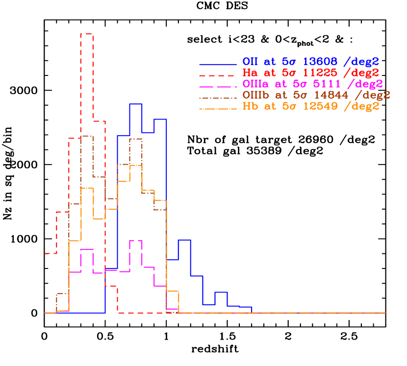
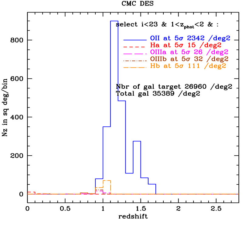
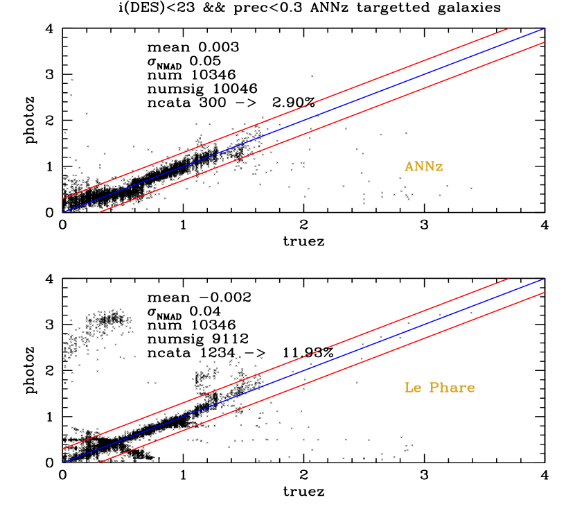
Figure 11: Example of the yield of a particular target-selection scheme based on the COSMOS Mock Catalogue (CMC) simulations. Here galaxies brighter than i=23 are selected that have photometric redshifts between 1 and 2 (left) and the full available number of targets is plotted in the middle panel, with photometric redshifts between 0 and 3. The left panel compares the photoz of ANNz and Le Phare.

Figure 11 shows that selection of high-redshift sources via photometric redshift is effective, and it shows that, as expected, [OII] is the principal spectroscopic feature in this range of redshifts. Furthermore all redshifts can be accessible with other lines including H$\alpha$, H$\beta$ and OIII. In Figure 11 we show the photometric redshifts plots for the same sample of galaxies. This should allow us to estimate the redshifts we miss due to the photo-z selection. For galaxies selected between redshifts 1 and 2 4.5% of galaxies are missed by this selection. i.e. 4.5% of galaxies will be outside the desired redshifts range. If we choose instead to select a low redshift emission line sample, the blunder rate with photo-z selection will be 12% of the galaxies.

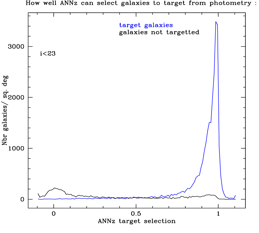
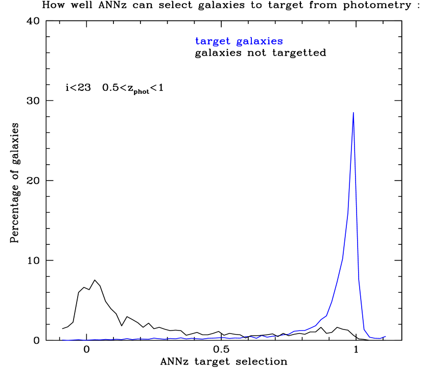
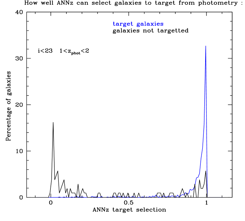
Figure 12: Histograms of ANNz target selection values for i$<$23 by deg2 with different photometric redshift selection. The middle and right figures are the same as the left figures with 0.5$<z_{phot}<$1 and 1$<z_{phot}<$2 for respectively the middle and right panels.

The blue line corresponds to the galaxies for which we will be able to measure a redshift, the “target galaxies”; they have at least one emission line detected at 5 sigma and we assign them a value of 1. The black line corresponds to the galaxies that do not have a strong emission line detectable, we assign them a value of 0. Using 10000 galaxies as a training sample, we derive ANNz target selection values.

If photo-z selection is applied we can select galaxies at high redshift with 95.5% of success and galaxies at intermediate redshifts (between 0.5 and 1) with 88% of success rate. DES photometry complemented with VHS photometry are assumed.

To define a selection criterion from the ANNz values, we draw the cumulative number of galaxies by deg2 as shown in Figure 13. A criterion of 0.8 select most of emission line galaxies and have a small contamination of weak or no emission line galaxies.

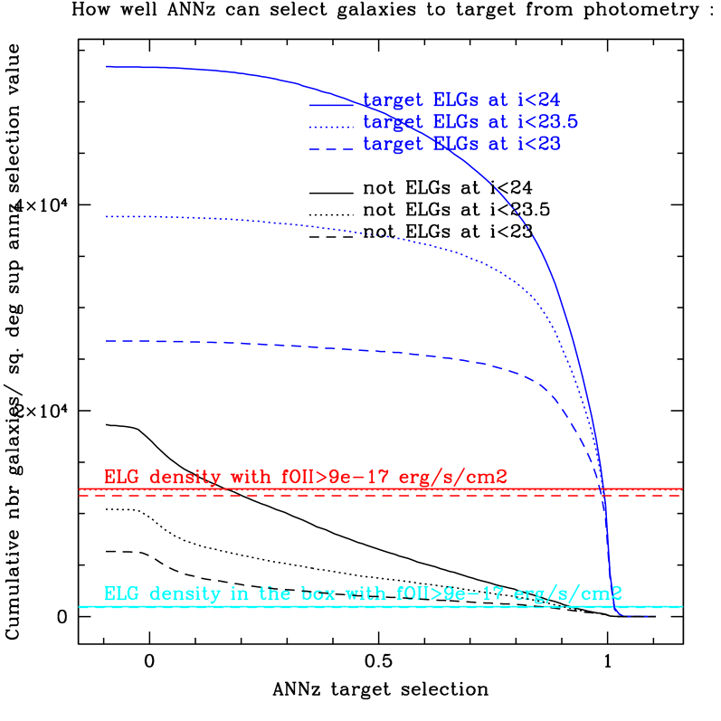
Figure 13: Cumulative number of galaxies/deg2 as a function of the ANNz target selection for ELGs. Using a ANNz target criterion of 0.8, we are able to reach a SSR of 95% at i$<$23 AB mag targeting close to 75% of all the galaxies at i$<$23. We will have a yield of 24000 galaxies/deg2.

6.3 Redshift distribution of color and NN selection for ELGs

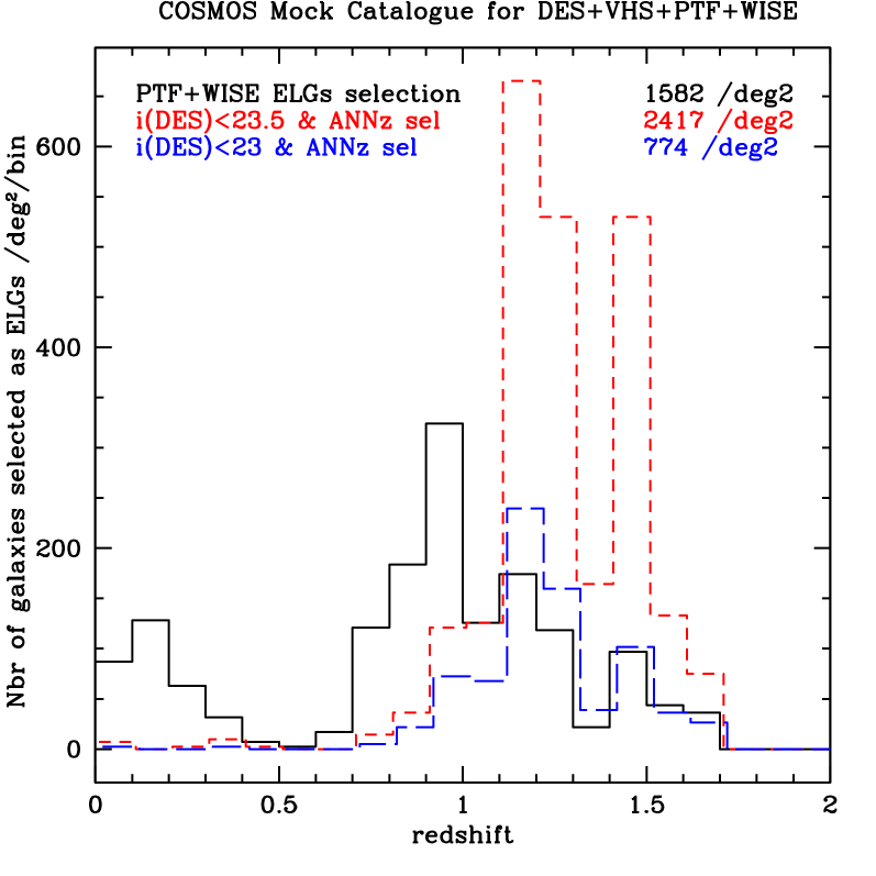
Figure 14: Redshift distribution for the color-color selection defined in Figure Figure 10. We add a selection function based on the photometric redshift in order to select galaxies at redshift higher than 0.5.

Figure 14 show ELGs redshifts distributions of the PTF+WISE color selection, and the DES+VHS NN selection at i brighter than 23 and 23.5 in respectively black solid, long-dashed blue and small-dashed red lines. The PTF+WISE curve include all the galaxies that are inside the box regardless of their type. The DES+VHS NN selection shows all the galaxies that have a NN value $>0.8$ and a selection function based on the photoz. We shape the redshift distribution in order to select all the high-redshift galaxies and have a smaller efficiency for the galaxies at lower redshift. We aim at to have a redshift distribution as flat as possible. Percival et al. shows that a flat redshift distribution gives the highest dark energy constraints.

In order to not be shot-noise limited, the target selection needs to yield 80gal/deg² by 0.1 bin in redshift. With the photoz selection function and the NN target selection, we will be able to study BAO up to z$\approx$ 1.7 without being shot-noise limited.

6.4 Spectroscopic Success Rate of color and NN selection for ELGs

We then derive the Spectroscopic Success Rate of ELGs for which we will be able to measure a redshift as shown in Figure 15. The dotted lines represent the SSR for different magnitude cut while the solid lines represent the percentage of galaxies compared to the total number of galaxies at the magnitude cut.

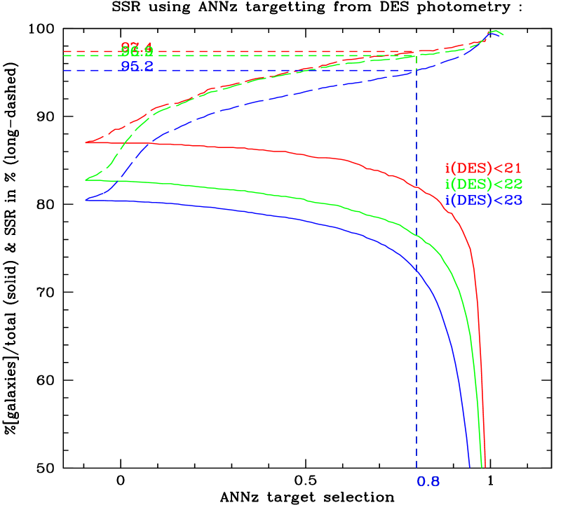
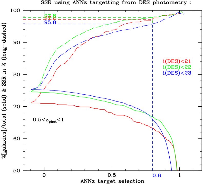
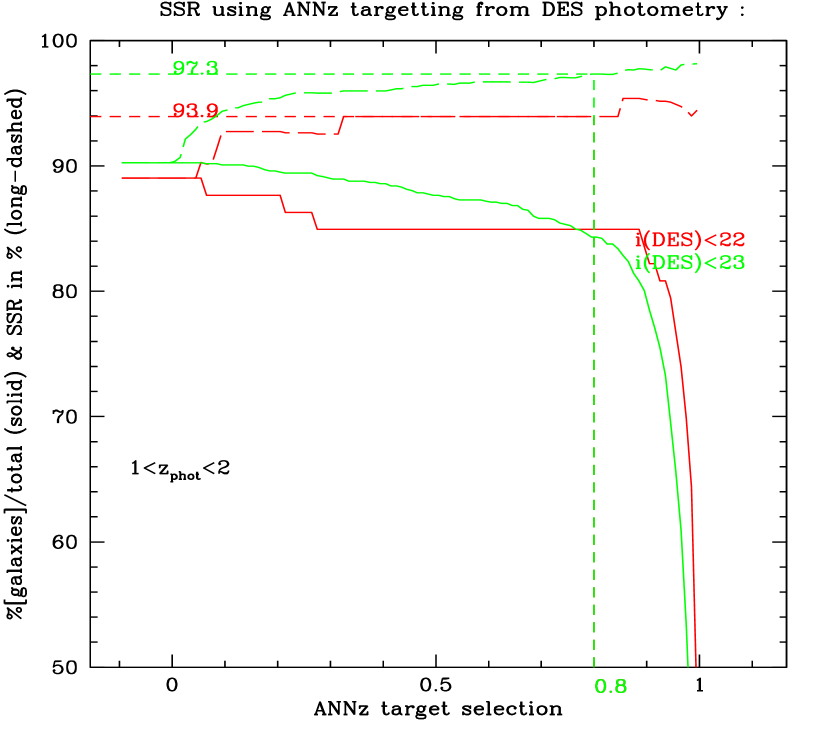
Figure 15: Spectroscopic Success Rate (dashed lines) and cumulative number of galaxies (solid lines) as a function of ANNz target selection values for a magnitude i$<$23 in blue, i$<$22 in green, and i$<$21 in red. The middle and right figures are the same as the left figures with 0.5$<z_{phot}<$1 and 1$<z_{phot}<$2 for respectively the middle and right panels.

7 Forecasts for Different Survey Strategy Assumptions

In this section and the next we present forecasts for our spectroscopic survey for a range of survey strategy and target selection options. Forecasts are made using the Fisher matrix formalism, described in section 7.1, then our choices for fiducial survey scenarios are outlined in section 7.1.1. Results are presented in section 8.

In this paper we concentrate on the effect of survey strategy on DE FoM (Albrecht et al. 2006), for a more detailed investigation of cosmological, astrophysical and systematic effects please see our companion paper Kirk et al. (2013).

7.1 Fisher formalism background

The forecasts in this section are calculated using the Fisher Matrix (FM) formalism (Kendall & Stuart 1977; Tegmark 1997). The FM is calculated as

$$F_{\alpha\beta}=\sum^{l_{max}}_{l=l_{min}}\sum_{(i,j),(m,n)}\frac{\partial D_{ij}(l)}{\partial p_{\alpha}}{\rm Cov}^{-1}\left[D_{ij}(l),D_{mn}(l)\right]\frac{\partial D_{mn}(l)}{\partial p_{\beta}}.$$ (1)

where $D_{ij}$ is the data vector for the observables under consideration, $\frac{\partial D_{mn}(l)}{\partial p_{\beta}}$ are the derivatives of this data vector with respect to the cosmological parameters, ${\rm Cov}\left[D_{ij}(l),D_{mn}(l)\right]$ is the covariance matrix of the data vector, calculated according to eqn. 39 of Joachimi & Bridle (2009).

For these forecasts we use projected angular power spectra, $C_{ij}(l)$s, as our observables. Each survey we consider is broken into a number of tomographic redshift bins and the auto-/cross-correlations of each of these bins is considered. The subscript $ij$ labels a tomographic bin-pair.

We consider forecasts for a galaxy survey with spectroscopic quality redshifts. In this case the data vector is simply the galaxy-galaxy $C(l)$s, i.e. $D_{ij}(l)=C^{nn}_{ij}(l)$. We also consider forecasts for a DES-like WGL survey with photometric quality redshifts. In this case the data vector is shear-shear power spectrum, i.e. $D_{ij}(l)=C^{\epsilon\epsilon}_{ij}(l)$. We consider combinations of these two surveys when there is no common overlap and when the two surveys fully overlap. In the no-overlap case the observables are independent and the separate FMs can simply be summed together. In the case of overlapping surveys we need to consider cross-correlations between the galaxy and shear observables. We calculate a single FM with data vector $D_{ij}(l)=\{C^{\epsilon\epsilon}_{ij}(l)C^{n\epsilon}_{ij}(l)C^{nn}_{ij}(l)\}$, where $C^{n\epsilon}_{ij}(l)$ are the galaxy-shear cross-correlations.

A general $C(l)$ is the projection of two window functions

$$C_{\alpha\beta}^{i,j}(l)=4\pi\int\Delta^{2}(k)W_{\alpha}^{i}(k)W_{\beta}^{j}(k)\frac{dk}{k}.$$ (2)

$W^{i}_{\alpha}(k)$ is the window function for tomographic bin $i$ and observable $\alpha$. In this document we consider three different $C(l)$ observables: $C_{nn}^{ij}(l)$, the galaxy-galaxy correlation (elsewhere called galaxy clustering), $C_{\epsilon\epsilon}^{ij}(l)$, the shear-shear correlation from WGL and $C_{n\epsilon}^{ij}(l)$, the galaxy-shear cross-correlation.

The weight function for galaxies is

$$\begin{split}W_{n}^{i}(l,k)&=\beta\int n(z(\chi))\Bigl{[}\frac{(2l^{2}+2l-1)}{(2l+3)(2l-1)}j_{l}(k\chi)-\\ &\frac{l(l-1)}{(2l-1)(2l+1)}j_{l-2}(k\chi)-\frac{(l+1)(l+2)}{(2l+1)(2l+3)}j_{l+2}(k\chi)\Bigr{]}d\chi,\end{split}$$ (3)

where $n^{i}(z)$ is the galaxy redshift distribution of tomographic bin $i$, $j_{l}(kz)$ is a bessel function and this expression includes the RSD formalism of Padmanabhan et al. (2005); Fisher et al. (1994).

For cosmic shear the weight function is

$$W_{\epsilon}^{i}(l,k)=\int\frac{3H_{0}^{2}\Omega_{m}}{2c^{2}}\frac{\chi}{a(\chi)}\int_{\chi_{hor}}^{\chi}p^{(i)}(\chi^{\prime})\frac{\chi^{\prime}-\chi}{\chi^{\prime}}d\chi^{\prime}j_{l}(k,\chi)d\chi.$$ (4)

We constrain the set of cosmological parameters $\left\{\Omega_{m},w_{0},w_{a},h,\sigma_{8},\Omega_{b},n_{s}\right\}$ which take the values $\Omega_{m}=0.25$, $w_{0}=-1$, $w_{a}=0$, $h=0.7$, $\sigma_{8}=0.8$, $\Omega_{b}=0.05$, $n_{s}=1$. All results assume a flat $\Lambda$CDM cosmology.

7.1.1 Survey Scenario Assumptions

For the purpose of these forecasts we describe two types of survey: a photometric WGL survey with photo-z quality redshifts and a spectroscopic survey with spec-z quality redshifts. For the spec-z survey we vary a number of properties to assess the impact of survey strategy and target selection. These choices are detailed below. We consider the properties of the photo-z survey to be fixed at the DES-reference values because we are primarily interested in the effect of choices in spec-z survey strategy on the combined photo-z + spec-z constraints.

The photometric survey is assumed to cover 5,000deg² with a galaxy number density of 10 arcmin^-2 ($\sim$ 300 million galaxies in total) and a redshift distribution given by the Smail-type $n(z)$,

$$n(z)=z^{\alpha}\exp{\left(-\left(\frac{z}{z_{0}}\right)^{\beta}\right)}$$ (5)

with $\alpha=2$, $\beta=1.5$, $z_{0}=0.9/\sqrt{2}$, divided into 5 tomographic bins with equal number density out to redshift 3 and normalised so that $\int n(z)dz=1$. A Gaussian photometric redshift error of $\sigma_{z}=0.07(1+z)$ was applied with no catastrophic outliers in redshift.

The photo-z survey has an area of 5,000deg² targetting $\sim$100 million galaxies (though both of these are varied, see below). The galaxy redshift distribution depends on choices of survey strategy and target selection described below but is assumed to cover redshifts from 0.4 to 1.7 and is split into 20 tomographic bins of equal z-range. We marginalise over our standard 7 cosmological parameters plus a galaxy bias model, $b_{g}(k,z)=A_{b_{g}}Q(k,z)$, which allows a variable overall amplitude term and a scale/redshift dependent grid parameterised with $2\times 2$ nodes in k/z. The fiducial values of the amplitude and scale/redshift nodes is unity. Our fiducial bias model is therefore also unity but our variable amplitude and grid nodes allow us to explore a range of flexible z- and k-dependent bias forms. These z/k-dependent biases are not tied to any specific models based on physical arguments or simulations, we are aiming in this case for maximum generality as a stringent test of our constraining power.

In section 8 we present forecasts for our spectroscopic survey alone and in combination with our photometric survey. Each spectroscopic forecast assumes a particular exposure time (from 20min to 50min) which, in turn, determines the total number of targets available in the telescope field of view, assumed to be 3deg². A longer exposure time allows fainter targets to be resolved hence a longer target list. Possible LRG and ELG targets are calculated independently. The spectrograph is assumed to have 3000 fibres covering the field of view allowing a maximum number of 1333 targets per square degree to be captured per exposure. If the number of available targets is less than this we assume the target list is saturated. If the number of possible targets is greater than the number of available fibres then a sub-set of 1333 galaxies are assumed to be captured at some specified ratio of LRG/ELG targets. Finally, for each forecast we assumed a total survey area (5000deg² - 15000deg²) and the number of times the area is tiled i.e. is each square degree of survey subject to a single exposure or does the telescope revisit multiple times. These multiple visits are useful when there are more available targets than fibres, allowing the excess to be captured on return visits. The combination of survey area, exposure time and number of tilings determines the total survey time in nights, assuming 8 hours observing per night. We assume a 90% success rate for spectral acquisition.

To summarise, the variables we consider in forecasting our spectroscopic survey are: i) exposure time, ii) LRG/ELG ratio, iii) number of tilings and iv) survey area.

8 Results

Here we present the results of our forecasts for a spec-z survey as a function of survey strategy and target selection choices. Throughout this section we will quote values for the Dark Energy Figure of Merit (DE FoM), based on the Dark Energy Task Force (Albrecht et al. 2006) definition

$$\textrm{FoM}_{\textrm{DE}}=\frac{1}{4\sqrt{\textrm{det}(F^{-1})_{\textrm{DE}}}},$$ (6)

where the subscript DE denotes the $2\times 2$ sub-matrix of the inverse FM that corresponds to the entries for the equation of state of DE parameters, $w_{0}$ and $w_{a}$. Note that different prefactors to this equation exist in the literature. We use the factor of $1/4$ for consistency with related papers (Bridle & King 2007; Joachimi & Bridle 2009).

This sort of FoM-based optimisation of surveys has been carried out numerous times including the examples of Bassett et al. (2005); Parkinson et al. (2007); Yamamoto et al. (2007); Parkinson et al. (2010); Paykari & Jaffe (2013); Kirk et al. (2011a); Amara & Réfrégier (2007).

8.1 FoM as a function of LRG/ELG ratio

Figure 16 shows the effect of selecting different ratios of LRG/ELG targets for a range of exposure times. Survey area is assumed fixed at 5000deg² and each forecast assumes one tiling of that area i.e. number density of galaxies is nowhere greater than 1333deg^-2.

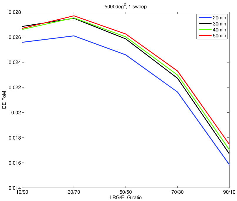
Figure 16: DE FoM as a function of LRG/ELG ratio for a range of exposure times. 5000deg² survey is assumed at all times and the area is tiled once. 7 cosmological parameters are marginalised over plus 5 galaxy bias parameters. Standard k-cuts assumed. *Possibly add survey time to legend*

It is clear that the trend with LRG/ELG ratio is robust across exposure times. The shortest exposure time, 20min, performs significantly worse than the others because such a short exposure with one tiling fails to saturate the number of available fibres with targets, resulting in significantly lower number densities. Even so the trend with target type is the same.

There is a clear peak at 30% LRG/ 70% LRG, while a strategy that focuses primarily on LRGs is clearly sub-optimal. ELGs predominate at high redshift so sacrificing them limits the volume of the survey. The inclusion of 30% LRGs seems sufficient to maintain good coverage across the z-range. Note we have not assumed each population to have a different galaxy bias. In practice ELGs are thought to be more strongly biased than LRGs. If biasing is equally well understood then more strongly biased populations are a more powerful probe of cosmology due to their larger signal to noise. This effect would enhance the trend seen on our results.

8.2 Area versus depth for fixed survey time

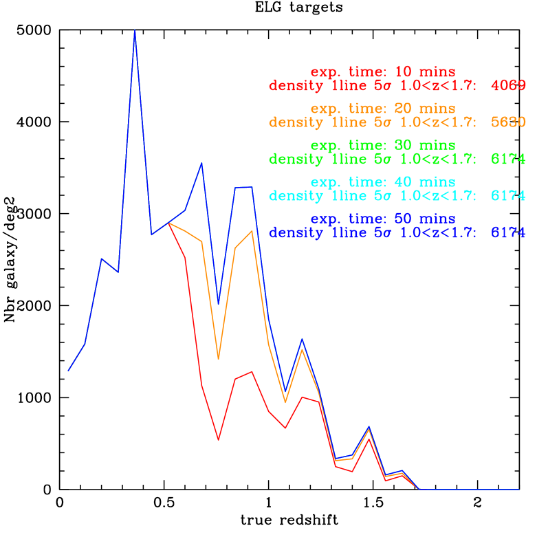
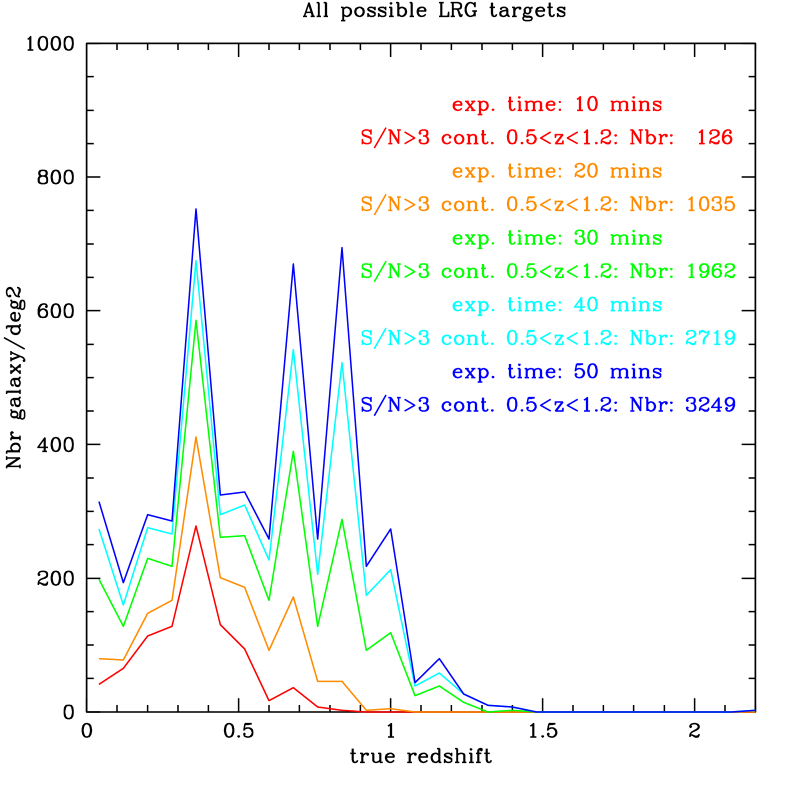
Figure 17: (Top panel) Redshift histograms for ELGs brighter than i $\sim$ 23.5. The different lines corresponds to successful redshifts obtained for different observation times. We note that the curves saturates after 30mins exposure as our photometric target selection is such that most emission lines are obtained.(Bottom panel) Redshifts histograms for LRGS brighter than i$\sim$ 22.

Figure 18 shows DE FoM as a function of survey area for a range of exposure times. The total survey time in nights is noted in the legend. To keep total survey time constant for each exposure time we trade off area and number of tilings. We assume 3 tilings for each 5000deg² forecast, 2 tilings for the 7,500deg² forecasts and a single tiling for the 15,000deg² forecasts. Some forecasts will be limited by the number of available fibres, 1,333deg^-2 per tiling, where this is less than the number of available targets. We do not forecast a 20min exposure time survey over 5000deg² with 3 tilings because the available target list is already saturated with 2 tilings so an additional pass would add nothing to a survey design.

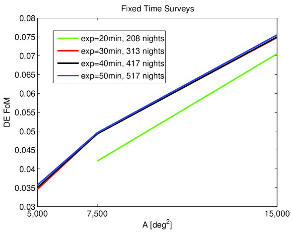
Figure 18: DE FoM as a function of exposure time for a 5000deg² survey where the area is tiled once. Where there are more targets than fibres an ELG/LRG ratio of 30/70 is assumed, otherwise the available target list is saturated. Total survey time in nights is noted beside each forecast point. Seven cosmological parameters are marginalised over plus 5 galaxy bias parameters. Standard k-cuts assumed.

More area is clearly beneficial, even at the cost of number density. This agrees with the findings of Amara & Réfrégier (2007) and Kirk et al. (2011b). 20min exposure times perform significantly worse due to their low number density. Above this level exposure time has little effect on the results because number density is limited by available fibres, changes in galaxy redshift distribution have a small effect, sub-dominant compared to the impact of number density/area.

8.3 Fixed Area, single survey sweep

In this section we forecast DE FoM for a 5000deg² survey as a function of exposure time, assuming the whole area is tiled once. Note that this means that, for exposure times of 20min and above, our acquired targets are limited by the 1,333 fibres per deg² available in our presumed instrument design.

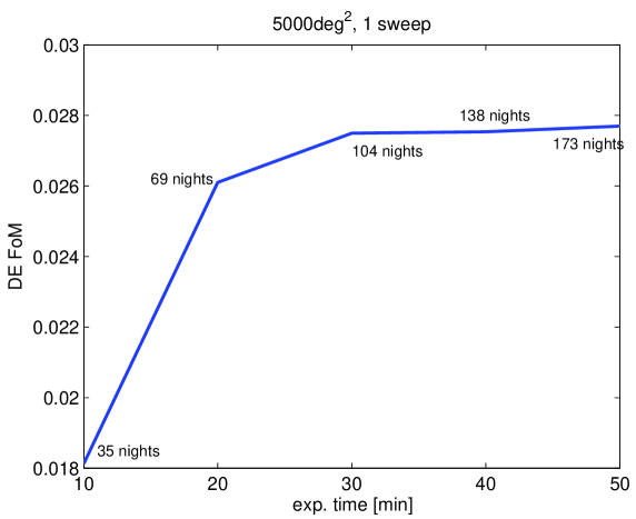
Figure 19: DE FoM as a function of exposure time. We assume a 5000deg² survey area which is tiled once. Total survey time in nights is noted next to each forecast. Where there are more targets than fibres an ELG/LRG ratio of 30/70 is assumed, otherwise the available target list is saturated. Seven cosmological parameters are marginalised over plus 5 galaxy bias parameters. Standard k-cuts assumed.

While DE FoM improves with increased exposure time, the majority of the available information is obtained by 20min exposure, with almost everything captured by 30min. This is due to the fact that number density, limited by number of fibres, is constant for 20min and above, any remaining benefit comes from the more even redshift distribution afforded by longer exposure times.

8.4 Fixed Area, full target list

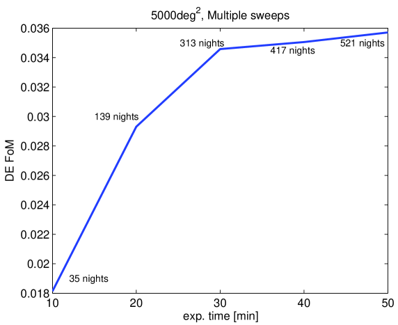
Figure 20: DE FoM as a function of exposure time. We assume a 5000deg² survey area which is tiled as many times as necessary to saturate the target list. This corresponds to 1 tiling for 20min exposures, 2 tilings for 20min and 30min exposures and 3 tilings for 40min and 50min exposures. Total survey time in nights is noted next to each forecast. Seven cosmological parameters are marginalised over plus 5 galaxy bias parameters. Standard k-cuts assumed.

When we fix our survey area to 5000deg² and allow enough tilings to saturate the target list for each exposure time we forecast the DE FoMs shown in Figure 20. Increased exposure time here leads to drastically increased total survey time as, not only does each individual pointing take more time, but entire 5000deg² tilings must be added if the number of available targets is greater than the number of available fibres. in practice we need 1 tiling for 10min exposure time, 2 tilings for 20min & 30min and 3 tilings for 40min & 50min.

The increased number density provided by exposure times of over 30min adds negligibly to the constraining power of the survey. A survey of $\sim 300$ nights captures almost all the available information. Note that there is some redundancy here as an entire extra tiling may not be the most profitable use of telescope time to catch a small number of targets missed due to lack of fibres on the previous tiling.

8.5 FoM as a function of wavelength

In this subsection, we investigate how the FoM changes depending on the maximum wavelength of the spectrograph. We can clearly see from the target selection plots that at high redshift most if not all the targets are obtained via the OII lines. Therefore there is a one-to-one relation between the maximum redshift that is achieved by our expereiemnt and the OII line dropping out of the range available by the spectrograph. We made simulations for the redshift histograms that can are obtainned spectroscopically for different detector cut offs and plotted the resulting distributions in Figure 21.

There is a significant amount of cosmic volume available at these redshifts and hence this redshift cutoff can significantly reduce the FOMs for Dark Energy recovery. We have calculated these FOM removing all information that is present at such redshifts and plotted the results in Figure 22. For reference the OII line is present at 3727 $\AA$ so a spectrograph which cuts off at 8000 $\AA$ would be able to detect OII out to $z\sim 1.14$ and a cutoff of 1 micron would correspond to OII at redshift 1.68. We can see from Figure 22 that the FOMs can cange by a factor of four by including these extra galaxies at high redshifts.

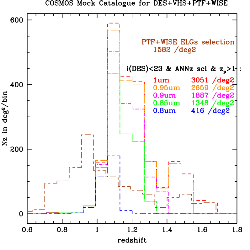
Figure 21: Nz of ELGs as a function of the spectrograph wavelength.

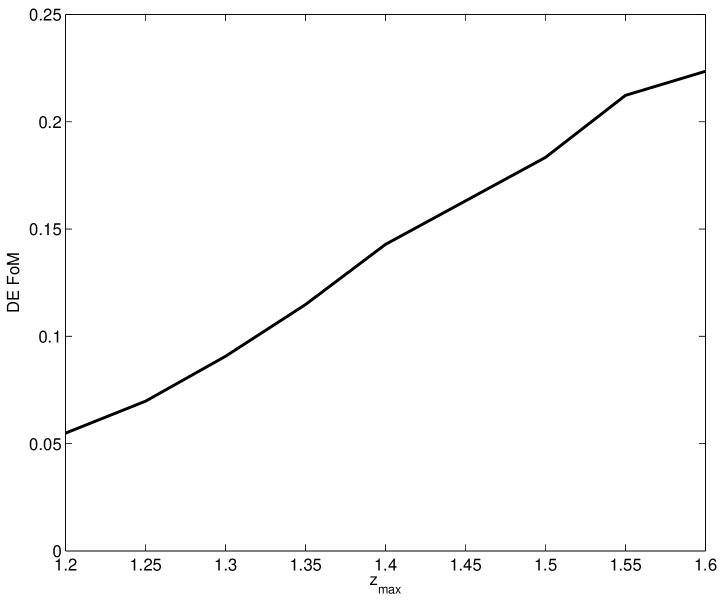
Figure 22: FoM as a function of the maximum redshift achievable by the spectroscopic instrument via the OII line.

9 Conclusion

In this paper we have produced a full forecast pipeline from realistic mock catalogues up to the DE FoM. With this pipeline we investigate several scenarios of spectroscopic survey design and seek to optimise that design in several ways. Using a spectroscopic instrument simulation similar to DESpec, BigBOSS or DESI, we first simulated a target selection strategy using shallow and deep photometry to cover the available range of current surveys such as DES, LSST, panSTARRS, PTF, WISE, VISTA. We have compared conservative color-color target selections and more complex ones based on neural network optimisation. We compare redshift distributions, success rate and completness of the target selections and find a very good results for the neural network selection.

We choose to target a mix of emission line galaxies and lyman red galaxies to cover the redshift range from 0.5 up to 1.7. For LRGs brighter than $i\sim 22$, we reach an SSR of 98% success for the neural network against 48 and 53% for color-color selections using respectively PTF-WISE and DES-VHS photometry. For the ELGs, we reach an SSR higher than 95% at magnitude i brighter than 23 for redshifts up to 1.3.

We thus show that having deep multicolor photometry for the target selection allows us to increase the number density of LRGs and ELGs targets by a factor of 2 to 3. It will also improve the efficiency and success rate of the target selection. Using the redshift distribution and target densities we find with the neural network selection, we give a first estimation of spectroscopic survey strategy. We look at tradeoff between ELG/LRG ratio survey area versus depth using FoM. The assumptions which go into the FoM calculation will be described in more detail in Kirk et al. (2013). We find a ratio of 30% LRG 70% ELG to be optimal when producing figures of merit for dark energy. Concerning the survey strategy, an exposure time shorter than 20mins is clearly sub-optimal and there is no significant benefit beyond 30mins. The optimal choice between these exposure times depends on survey strategy choices, area versus completness of the target list. The procedure presented in this paper is a general approach. We are able to use it to optimise the target selectio and survey strategy for any future spectroscopic and overlapping photometric surveys

10 Acknowledgements

The authors thank the DESpec collaboration for their useful discussions which help developping this work. Funding for this project was partially provided by the Spanish project AYA2009-13936, Consolider-Ingenio CSD2007- 00060, EC Marie Curie Initial Training Network CosmoComp (PITN-GA-2009-238356) and research project 2009- SGR-1398 from Generalitat de Catalunya. FBA thanks the Royal Society for support via an URF.

References

- Abdalla et al. (2012) Abdalla F., Annis J., Bacon D., Bridle S., Castander F., Colless M., DePoy D., Diehl H. T., Eriksen M., Flaugher B., Frieman J., Gaztanaga E. e. a., 2012, ArXiv e-prints
- Abdalla et al. (2008) Abdalla F. B., Amara A., Capak P., Cypriano E. S., Lahav O., Rhodes J., 2008, MNRAS, 387, 969
- Abdalla et al. (2008) Abdalla F. B., Mateus A., Santos W. A., Sodrè Jr. L., Ferreras I., Lahav O., 2008, MNRAS, 387, 945
- Albrecht et al. (2006) Albrecht A., Bernstein G., Cahn R., Freedman W. L., Hewitt J., Hu W., Huth J., Kamionkowski M., Kolb E. W., Knox L., Mather J. C., Staggs S., Suntzeff N. B., 2006, ArXiv Astrophysics e-prints
- Amara & Réfrégier (2007) Amara A., Réfrégier A., 2007, MNRAS, 381, 1018
- Banerji et al. (2008) Banerji M., Abdalla F. B., Lahav O., Lin H., 2008, MNRAS, 386, 1219
- Bassett et al. (2005) Bassett B. A., Parkinson D., Nichol R. C., 2005, ApJ, 626, L1
- Blake et al. (2012) Blake C., Brough S., Colless M., Contreras C., Couch W., Croom S., Croton D., Davis T. M., Drinkwater M. J., Forster K., Gilbank D. e. a., 2012, MNRAS, 425, 405
- Blanton & Roweis (2007) Blanton M. R., Roweis S., 2007, AJ, 133, 734
- Bridle & King (2007) Bridle S., King L., 2007, New Journal of Physics, 9, 444
- Bruzual & Charlot (2003) Bruzual G., Charlot S., 2003, MNRAS, 344, 1000
- Capak et al. (2007) Capak P., Aussel H., Ajiki M., McCracken H. J., Mobasher B., Scoville N., Shopbell P., Taniguchi Y. e. a., 2007, ApJS, 172, 99
- Capak et al. (2008) Capak P., Aussel H., Ajiki M., McCracken H. J., Mobasher B., Scoville N., Shopbell P., Taniguchi Y. e. a., 2008, VizieR Online Data Catalog, 2284, 0
- Coe et al. (2006) Coe D., Benítez N., Sánchez S. F., Jee M., Bouwens R., Ford H., 2006, AJ, 132, 926
- Collister & Lahav (2004) Collister A. A., Lahav O., 2004, PASP, 116, 345
- Dawson et al. (2013) Dawson K. S., Schlegel D. J., Ahn C. P., Anderson S. F., Aubourg É., Bailey S., Barkhouser R. H. e. a., 2013, AJ, 145, 10
- de Jong et al. (2012) de Jong R. S., Bellido-Tirado O., Chiappini C., Depagne É., Haynes R., Johl D., Schnurr O. e. a., 2012, in Society of Photo-Optical Instrumentation Engineers (SPIE) Conference Series Vol. 8446 of Society of Photo-Optical Instrumentation Engineers (SPIE) Conference Series, 4MOST: 4-metre multi-object spectroscopic telescope
- Drinkwater et al. (2010) Drinkwater M. J., Jurek R. J., Blake C., Woods D., Pimbblet K. A., Glazebrook K., Sharp R., Pracy M. B., Brough S., Colless M., Couch W. J., Croom S. M. e. a., 2010, MNRAS, 401, 1429
- Eisenstein et al. (2001) Eisenstein D. J., Annis J., Gunn J. E., Szalay A. S., Connolly A. J., Nichol R. C., Bahcall N. A. e. a., 2001, AJ, 122, 2267
- Fisher et al. (1994) Fisher K. B., Scharf C. A., Lahav O., 1994, MNRAS, 266, 219
- Gaztañaga et al. (2012) Gaztañaga E., Eriksen M., Crocce M., Castander F. J., Fosalba P., Marti P., Miquel R., Cabré A., 2012, MNRAS, 422, 2904
- Giavalisco et al. (2004) Giavalisco M., Ferguson H. C., Koekemoer A. M., Dickinson M., Alexander D. M., Bauer F. E. e. a., 2004, ApJ, 600, L93
- Ilbert et al. (2009) Ilbert O., Capak P., Salvato M., Aussel H., McCracken H. J., Sanders D. B., Scoville N. e. a., 2009, ApJ, 690, 1236
- Joachimi & Bridle (2009) Joachimi B., Bridle S. L., 2009, ArXiv e-prints
- Jouvel et al. (2009) Jouvel S., Kneib J.-P., Ilbert O., Bernstein G., Arnouts S., Dahlen T., Ealet A., Milliard B., Aussel H., Capak P., Koekemoer A., Le Brun V., McCracken H., Salvato M., Scoville N., 2009, A&A, 504, 359
- Kendall & Stuart (1977) Kendall M., Stuart A., 1977, The advanced theory of statistics. Vol.1: Distribution theory
- Kennicutt (1998) Kennicutt Jr. R. C., 1998, ARA&A, 36, 189
- Kirk et al. (2013) Kirk D., Lahav O., Bridle S., Jouvel S., Abdalla F. B., Frieman J. A., 2013, ArXiv e-prints
- Kirk et al. (2011a) Kirk D., Laszlo I., Bridle S., Bean R., 2011a, ArXiv e-prints
- Kirk et al. (2011b) Kirk D., Laszlo I., Bridle S., Bean R., 2011b, ArXiv e-prints
- Le Fèvre et al. (2005) Le Fèvre O., Vettolani G., Garilli B., Tresse L., Bottini D., Le Brun V., Maccagni D. e. a., 2005, A&A, 439, 845
- Martin et al. (2005) Martin D. C., Fanson J., Schiminovich D., Morrissey P., Friedman P. G., Barlow T. A. Conrow T., Grange R., Jelinsky P. N., Milliard B. e. a., 2005, ApJ, 619, L1
- McCall et al. (1985) McCall M. L., Rybski P. M., Shields G. A., 1985, ApJS, 57, 1
- Mouhcine et al. (2005) Mouhcine M., Lewis I., Jones B., Lamareille F., Maddox S. J., Contini T., 2005, MNRAS, 362, 1143
- Moustakas et al. (2006) Moustakas J., Kennicutt Jr. R. C., Tremonti C. A., 2006, ApJ, 642, 775
- Padmanabhan et al. (2005) Padmanabhan N., Budavári T., Schlegel D. J., Bridges T., Brinkmann J., Cannon R., Connolly A. J. e. a., 2005, MNRAS, 359, 237
- Parkinson et al. (2007) Parkinson D., Blake C., Kunz M., Bassett B. A., Nichol R. C., Glazebrook K., 2007, MNRAS, 377, 185
- Parkinson et al. (2010) Parkinson D., Kunz M., Liddle A. R., Bassett B. A., Nichol R. C., Vardanyan M., 2010, MNRAS, 401, 2169
- Paykari & Jaffe (2013) Paykari P., Jaffe A. H., 2013, MNRAS, 433, 3523
- Polletta et al. (2007) Polletta M., Tajer M., Maraschi L., Trinchieri G., Lonsdale C. J., Chiappetti L., Andreon S. e. a., 2007, ApJ, 663, 81
- Reid et al. (2012) Reid B. A., Samushia L., White M., Percival W. J., Manera M., Padmanabhan N., Ross A. J., Sánchez A. G., Bailey S., Bizyaev D., Bolton A. S., Brewington H. e. a., 2012, MNRAS, 426, 2719
- Schlegel et al. (2011) Schlegel D., Abdalla F., Abraham T., Ahn C., Allende Prieto C., Annis J., Aubourg E., Azzaro M. e. a., 2011, ArXiv e-prints
- Tegmark (1997) Tegmark M., 1997, Physical Review Letters, 79, 3806
- Yamamoto et al. (2007) Yamamoto K., Parkinson D., Hamana T., Nichol R. C., Suto Y., 2007, Phys. Rev. D, 76, 023504
- Zoubian & Kneib (2013) Zoubian J., Kneib J.-P. e. a., 2013