Statistical and other properties of Riemann zeros based on an explicit equation for the $n$-th zero on the critical line

Abstract

We show that there are an infinite number of Riemann zeros on the critical line, enumerated by the positive integers $n=1,2,\dotsc$, whose ordinates can be obtained as the solution of a new transcendental equation that depends only on $n$. Under weak assumptions, we show that the number of such zeros already saturates the counting formula for the numbers of zeros on the entire critical strip. These results thus constitute a concrete proposal toward verifying the Riemann hypothesis. We perform numerical analyses of the exact equation, and its asymptotic limit of large ordinate. The starting point is an explicit analytical formula for an approximate solution to the exact equation in terms of the Lambert $W$ function. In this way, we neither have to use Gram points or deal with violations of Gram’s law. Our numerical approach thus constitutes a novel method to compute the zeros. Employing these numerical solutions, we verify that solutions of the asymptotic version are accurate enough to confirm Montgomery’s and Odlyzko’s pair correlation conjectures and also to reconstruct the prime number counting function.

I Introduction

Riemann’s major contribution to number theory was an explicit formula for the arithmetic function $\pi(x)$, which counts the number of primes less than $x$, in terms of an infinite sum over the non-trivial zeros of the $\zeta(z)$ function, i.e. roots $\rho$ of the equation $\zeta(z)=0$ on the critical strip $0\leq\Re(z)\leq 1$ Edwards . It was later proven by Hadamard and de la Vallée Poussin that there are no zeros on the line $\Re(z)=1$, which in turn proved the Prime Number Theorem $\pi(x)\sim{\rm Li}(x)$. (See section VI for a review.) Hardy proved that there are an infinite number of zeros on the critical line $\Re(z)=\tfrac{1}{2}$. The Riemann hypothesis (RH) was his statement, in 1859, that all zeros on the critical strip have $\Re(\rho)=\tfrac{1}{2}$, although he was unable to prove it. Despite strong numerical evidence of its validity, it remains unproven to this day. Many important mathematical results were proven assuming the RH, so it is a cornerstone of fundamental mathematics. Some excellent introductions to the RH are Conrey ; Sarnak ; Bombieri .

Throughout this paper, the argument of the $\zeta(z)$ function will be the complex number $z=x+iy$, and zeros will be denoted as $\rho$. We need only consider the positive $y$-axis, since if $\rho$ is a zero so is its complex conjugate. The infinite zeros along the critical line can be numbered as one moves up the $y$-axis, $\rho_{n}=\tfrac{1}{2}+iy_{n}$. The first few are $y_{1}\simeq 14.1347$, $y_{2}\simeq 21.0220$ and $y_{3}\simeq 25.0108$. Although at first sight there doesn’t appear to be any regular pattern to these zeros, we will demonstrate in this paper that they have a universal description: there are in one-to-one correspondence with the zeros of the cosine function.

Riemann gave an estimate $N(T)$ for the average number of zeros on the entire critical strip with imaginary part between $0$ and $T$. If $T$ does not correspond to the ordinate of a zero, when $T\to\infty$ we have Edwards ; Titchmarsh

$$N(T)=\dfrac{T}{2\pi}\log\left(\dfrac{T}{2\pi e}\right)+\dfrac{7}{8}+O\left(\log T\right).$$ (1)

This formula was later proven by von Mangoldt, but has it never been proven to be valid on the critical line, as explicitly stated in Edward’s book Edwards . Denoting the zeros on the critical line by $N_{0}(T)$, Hardy and Littlewood showed that $N_{0}(T)>C\,T$ and Selberg improved this result stating that $N_{0}(T)>C\,T\log T$ for very small $C$. Then, Levinson Levinson demonstrated that $N_{0}(T)\geq CN(T)$ where $C=\tfrac{1}{3}$. The current most precise result is due to Conrey Conrey2 who improved the last result demonstrating that $C=\tfrac{2}{5}$. Obviously, if the RH is true then $N_{0}(T)=N(T)\sim\tfrac{T}{2\pi}\log\tfrac{T}{2\pi}-\tfrac{T}{2\pi}$. These statements are described in (Edwards, , Chapter 11) and (Titchmarsh, , Chapter X). The formula (1) can be seen as an asymptotic expansion of an exact formula due to Backlund, who proved the following result also on the critical strip (Edwards, , Chapter 6):

$$N(T)=\dfrac{1}{\pi}\vartheta(T)+1+S(T),$$ (2)

where we have the Riemann-Siegel $\vartheta$ function (introduced in section II.2) and $S(T)=\tfrac{1}{\pi}\arg\zeta(\tfrac{1}{2}+iT)$. Using the well known expansion $\vartheta(T)=\tfrac{T}{2}\log\left(\tfrac{T}{2\pi e}\right)-\tfrac{\pi}{8}+O\left(T^{-1}\right)$ one recovers (1) from (2).

Montgomery’s conjecture that the non-trivial zeros satisfy the statistics of the eigenvalues of random hermitian matrices Montgomery led Berry to propose that the zeros are eigenvalues of a chaotic hamiltonian Berry1 , along the lines of the original Hilbert-Polya idea. Further developments are in BerryKeating ; BerryKeating2 ; Sierra ; Sierra2 ; Bhaduri . These works focus on $N(T)$, and carry out the analysis on the critical line, i.e. they essentially assume the validity of the RH. A number of interesting analytic results were obtained, emphasizing the important role of the function $\arg\zeta\left(\tfrac{1}{2}+iT\right)$. In a related, but essentially different approach by Connes based on adeles, there exists an operator playing the role of the hamiltonian, which has a continuous spectrum, and the Riemann zeros correspond to missing spectral lines Connes . We mention these interesting works because of the role of $N(T)$ in them, however, we will not be pursuing these ideas in this work. For interesting connections of the RH to physics see Connes2 ; Schumayer (and references therein).

Riemann’s counting formula (1) counts zeros very accurately if one takes into account the term $\tfrac{1}{\pi}\arg\zeta\left(\tfrac{1}{2}+iT\right)$. Thus, it is not a smooth function but jumps by one at each zero on the critical line. This “fluctuating term” is discussed in some detail in Berry1 ; BerryKeating . If in some region of the critical strip one can show that the counting formula $N(T)$ correctly counts the zeros on the critical line, then this proves the RH in this region of the strip. Since it has been shown numerically that the first billion or so zeros all lie on the critical line deLune ; Gourdon , one approach to establishing the RH is to develop an asymptotic approximation and show that there are no zeros off of the critical line for sufficiently large $y$. Such an analysis was carried out in RHLeclair where the main outcome was an asymptotic equation for the $n$-th zero on the critical line, $\rho_{n}=\tfrac{1}{2}+iy_{n}$, where $y_{n}$ satisfies the transcendental equation (14) below. The way in which this equation is derived shows that these zeros are in one-to-one correspondence with the zeros of the cosine function; it is in this manner that the $n$-dependence arises. As will be shown in this paper, the numerical solutions to this equation unexpectedly accurately correspond to the already well known values for $y_{n}$ Odlyzko , even for the lowest zeros.

More importantly, since these equations for zeros on the critical line are enumerated by the integer $n$, one can use them to obtain the counting of such zeros, which we continue to denote as $N_{0}(T)$. Comparing with Riemann’s counting formula (1) for the number of zeros on the entire critical strip, we will argue that $N_{0}(T)=N(T)$, first asymptotically, then exactly, based on the exact equation (20).

Our work presents a novel method to compute the Riemann zeros. We first obtain an explicit formula as an approximate solution for $y_{n}$, in terms of the Lambert $W$ function. Starting from this approximation we obtain accurate numerical solutions of (14), which is the simplest approximation to (20). We show that these numerical solutions are accurate enough to verify Montgomery’s and Odlyzko’s pair correlation conjectures, and also to reconstruct the prime number counting formula. We emphasize that our numerical approach does not make use of Gram points nor the Riemann-Siegel $Z$ function, and we believe is actually simpler than the standard methods.

Let us anticipate a possible misunderstanding or criticism due to the resemblance between (14) and (1), and also between (20) and (2). We stress that our results were derived directly on the critical line, without assuming the RH. Furthermore, (14) and (20) are not counting formulas. Rather, they are equations that determine the imaginary parts $y_{n}$’s of the Riemann zeros. In other words, the $n$-th Riemann zero is the solution of these equations. Whereas the simple equation $\zeta(\rho)=0$ has an infinite number of solutions, equations (14) and (20) have a single solution for each $n$. We remind the reader that formulas (1) and (2) were derived on the entire critical strip, moreover, assuming that $T$ is not the ordinate of a zero. Thus, it is impossible to derive (14) from (1), nor (20) from (2). The equations (14) and (20) are new equations that are fundamentally different in meaning, and stronger, than the known counting formulas. We have been unable to find them in the literature.

We organize our work as follows. Section II contains our main results. More precisely, we derive an exact equation satisfied by each individual Riemann zero on the critical line. The asymptotic limit of this equation is the equation first proposed in RHLeclair , however we provide a more rigorous and thorough analysis. In section III we obtain an approximate solution for the ordinates of the zeros on the critical line, as an explicit formula. This provides the starting point to compute accurate numerical solutions, shown in section IV. In section V we verify the Montgomery-Odlyzko pair correlation conjecture, based on our numerical solutions of the asymptotic version. Also, in section VI we reconstruct the prime number counting function, again based on solutions of the asymptotic approximation of the exact equation. Section VII presents some numerical solutions to the exact equation, which proved to be much more robust under the numerical methods. Finally, in section VIII, we present our concluding remarks.

II An equation for the Riemann zeros on the critical line

In this section we derive the exact equation (20) for the $n$-th Riemann zero, which is our main result. In the first sub-section we present its asymptotic version (14), first proposed in RHLeclair , since it involves more familiar functions; this first sub-section should be viewed as following trivially from the second sub-section.

II.1 Asymptotic equation

Let us start by defining the function

$$\chi(z)\equiv\pi^{-z/2}\Gamma\left(z/2\right)\zeta(z).$$ (3)

In quantum statistical physics, this function is the free energy of a gas of massless bosonic particles in $d$ spatial dimensions when $z=d+1$, up to the overall power of the temperature $T^{d+1}$. Under a “modular” transformation that exchanges one spatial coordinate with Euclidean time, if one analytically continues $d$, physical arguments AL shows that it must have the symmetry

$$\chi\left(z\right)=\chi\left(1-z\right).$$ (4)

This is the fundamental, and amazing, functional equation satisfied by the $\zeta(z)$ function, which was proven by Riemann. For several different ways of proving (4) see Titchmarsh . Now consider Stirling’s approximation, $\Gamma(z)=\sqrt{2\pi}z^{z-1/2}e^{-z}\left(1+O\left(z^{-1}\right)\right)$, where $z=x+iy$, which is valid for large $y$. Under this condition we also have

$$z^{z}=\exp\left(i\left(y\log y+\dfrac{\pi x}{2}\right)+x\log y-\dfrac{\pi y}{2}+x+O\left(y^{-1}\right)\right).$$ (5)

Therefore, using the polar representation $\zeta=|\zeta|e^{i\arg\zeta}$ and the above expansions, we can write $\chi=A\,e^{i\theta}$ where

$$A(x,y) =\sqrt{2\pi}\,\pi^{-x/2}\left(\dfrac{y}{2}\right)^{(x-1)/2}e^{-\pi y/4}|\zeta(x+iy)|\left(1+O\left(z^{-1}\right)\right),$$ (6)

$$\theta(x,y) =\dfrac{y}{2}\log\left(\dfrac{y}{2\pi e}\right)+\dfrac{\pi}{4}(x-1)+\arg\zeta(x+iy)+O\left(y^{-1}\right).$$ (7)

The above approximation is very accurate. For $y$ as low as $100$, it evaluates $\chi\left(\tfrac{1}{2}+iy\right)$ correctly to one part in $10^{6}$.

Now let $\rho=x+iy$ be a Riemann zero. Then $\arg\zeta(\rho)$ can be well-defined by the limit

$$\arg\zeta\left(\rho\right)\equiv\lim_{\delta\to 0^{+}}\arg\zeta\left(x+\delta+iy\right).$$ (8)

Note that $0<\delta\ll 1$. This limit in general is not zero. For instance, for the first Riemann zero, $\arg\zeta\left(\tfrac{1}{2}+iy_{1}\right)\simeq 0.1578739$. On the critical line $z=\tfrac{1}{2}+it$, if $t$ does not correspond to the imaginary part of a zero, the well known function $S(t)=\tfrac{1}{\pi}\arg\zeta\left(\tfrac{1}{2}+it\right)$, already mentioned in connection with (1) and (2), is defined by continuous variation along the straight lines starting from $2$, then up to $2+it$ and finally to $\tfrac{1}{2}+it$, where $\arg\zeta(2)=0$. Assuming the RH, the current best bound is given by $|S(t)|\leq\left(\tfrac{1}{2}+o(1)\right)\tfrac{\log t}{\log\log t}$ for $t\to\infty$, proven by Goldston and Gonek Goldston . On a zero, the standard way to define this term is through the limit $S(\rho)=\tfrac{1}{2}\lim_{\epsilon\to 0}\left(S\left(\rho+i\epsilon\right)+S\left(\rho-i\epsilon\right)\right)$. We have checked numerically that for several zeros on the line, our definition (8) gives the same answer as this standard approach.

From (3) we have $\left(\chi(z)\right)^{*}=\chi\left(z^{*}\right)$, thus $A(x,-y)=A(x,y)$ and $\theta(x,-y)=-\theta(x,y)$. Denoting $\chi\left(1-z\right)\equiv A^{\prime}\,e^{-i\theta^{\prime}}$ this implies that

$$A^{\prime}(x,y)=A(1-x,y),\qquad\theta^{\prime}(x,y)=\theta(1-x,y).$$ (9)

From (4) we also have $|\chi(z)|=|\chi(1-z)|$, therefore $A(x,y)=A^{\prime}(x,y)$ for any $z$ on the critical strip.

Now let us consider what happens when we approach a zero $\rho=x+iy$ through a limit. From (3) it follows that $\zeta(z)$ and $\chi(z)$ have the same zeros on the critical strip, so it is enough to consider the zeros of $\chi(z)$. From (4) we see that if $\rho$ is a zero so is $1-\rho$. Then we clearly have

$$\lim_{\delta\to 0^{+}}\left[\chi(\rho+\delta)+\chi(1-\rho-\delta)\right]=\lim_{\delta\to 0^{+}}A(x+\delta,y)B(x+\delta,y)=0,$$ (10)

where

$$B(x,y)\equiv e^{i\theta(x,y)}+e^{-i\theta^{\prime}(x,y)}.$$ (11)

The second equality in (10) follows from $A=A^{\prime}$. Then, in the limit $\delta\to 0^{+}$, a zero corresponds to $A=0$, $B=0$ or both. They can simultaneously be zero since they are not independent. If $B=0$ then $A=0$, since $A\propto|\zeta(z)|$. However, the converse is not necessarily true.

Since there is more structure in $B$, let us consider $B=0$. The general solution of this equation is given by $\theta+\theta^{\prime}=(2n+1)\pi$, which are a family of curves $y(x)$. However, since $\chi(z)$ is an analytic function, we know that the zeros must be isolated points rather than curves, and this general solution must be restricted. Thus, let us choose the particular solution

$$\theta=\theta^{\prime},\qquad\lim_{\delta\to 0^{+}}\cos\theta=0.$$ (12)

On the critical line, the first equation (12) is already satisfied. Now, in the limit $\delta\to 0^{+}$, the second equation implies $\theta=\left(n+\tfrac{1}{2}\right)\pi$, for $n=0,\pm 1,\pm 2,\dotsc$, hence

$$n=\dfrac{y}{2\pi}\log\left(\dfrac{y}{2\pi e}\right)-\dfrac{5}{8}+\lim_{\delta\to 0^{+}}\dfrac{1}{\pi}\arg\zeta\left(\tfrac{1}{2}+iy+\delta\right).$$ (13)

A closer inspection shows that the right hand side of (13) has a minimum in the interval $(-2,-1)$, thus $n$ is bounded from below, i.e. $n\geq-1$. Establishing the convention that zeros are labeled by positive integers, $\rho_{n}=\tfrac{1}{2}+iy_{n}$ where $n=1,2,\dotsc$, we must replace $n\to n-2$ in (13). Therefore, the imaginary parts of these zeros are determined from the solution of the transcendental equation

$$\dfrac{y_{n}}{2\pi}\log\left(\dfrac{y_{n}}{2\pi e}\right)+\lim_{\delta\to 0^{+}}\dfrac{1}{\pi}\arg\zeta\left(\tfrac{1}{2}+\delta+iy_{n}\right)=n-\dfrac{11}{8}\qquad(n=1,2,\dotsc).$$ (14)

In short, we have shown that, asymptotically, there are an infinite number of zeros on the critical line whose ordinates can be determined by solving (14) for $y_{n}$.

Note that, by comparing with the counting function $N(T)$, the left hand side of (14) is a monotonic increasing function of $y$, and the leading term is a smooth function. Possible discontinuities can only come from $\tfrac{1}{\pi}\arg\zeta\left(\tfrac{1}{2}+iy\right)$, and in fact, it has a jump discontinuity by one whenever $y$ corresponds to a zero. However, if $\lim_{\delta\to 0^{+}}\arg\zeta\left(\tfrac{1}{2}+\delta+iy\right)$ is well defined, then the left hand side of equation (14) is well defined for any $y$ and there is a unique solution for every $n$. Under this assumption, the number of solutions of equation (14), up to height $T$, is given by

$$N_{0}(T)=\dfrac{T}{2\pi}\log\left(\dfrac{T}{2\pi e}\right)+\dfrac{7}{8}+\dfrac{1}{\pi}\arg\zeta\left(\tfrac{1}{2}+iT\right)+O\left(T^{-1}\right).$$ (15)

This is so because the zeros are already numbered in (14), but the left hand side jumps by one at each zero, with values $-1/2$ to the left and $+1/2$ to the right of the zero. Thus we can replace $n\to N_{0}+1/2$ and $y_{n}\to T$, such that the jumps correspond to integer values. In this way $T$ will not correspond to the ordinate of a zero and $\delta$ can be eliminated.

Let us now recall the Riemann-von Mangoldt formula (1) for the number of zeros on the critical strip. It is the same as the number of zeros on the critical line that we have just found (15), i.e. $N_{0}(T)=N(T)$. This means that our particular solution (12), leading to equation (14), already saturates the counting formula on the whole strip and there are no additional zeros from $A=0$ in (10) nor from the general solution $\theta+\theta^{\prime}=(2n+1)\pi$. This strongly suggests that (14) describes all the non-trivial zeros, which are all on the critical line.

II.2 Exact equation

Let us now reproduce the same analysis discussed previously but without an asymptotic expansion. The exact versions of (6) and (7) are

$$A(x,y) =\pi^{-x/2}|\Gamma\left(\tfrac{1}{2}(x+iy)\right)||\zeta(x+iy)|,$$ (16)

$$\theta(x,y) =\arg\Gamma\left(\tfrac{1}{2}(x+iy)\right)-\dfrac{y}{2}\log\pi+\arg\zeta(x+iy),$$ (17)

where again $\chi(z)=Ae^{i\theta}$ and $\chi(1-z)=A^{\prime}e^{-i\theta}$, with $A^{\prime}(x,y)=A(1-x,y)$ and $\theta^{\prime}(x,y)=\theta(1-x,y)$. The zeros on the critical line correspond to the particular solution $\theta=\theta^{\prime}$ and $\lim_{\delta\to 0^{+}}\cos\theta=0$. Thus $\lim_{\delta\to 0^{+}}\theta=\left(n+\tfrac{1}{2}\right)\pi$ and replacing $n\to n-2$, the imaginary parts of these zeros must satisfy the exact equation

$$\arg\Gamma\left(\tfrac{1}{4}+\tfrac{i}{2}y_{n}\right)-y_{n}\log\sqrt{\pi}+\lim_{\delta\to 0^{+}}\arg\zeta\left(\tfrac{1}{2}+iy_{n}\right)=\left(n-\tfrac{3}{2}\right)\pi.$$ (18)

The Riemann-Siegel $\vartheta$ function is defined by

$$\vartheta(t)\equiv\arg\Gamma\left(\tfrac{1}{4}+\tfrac{i}{2}t\right)-t\log\sqrt{\pi},$$ (19)

where the argument is defined such that this function is continuous and $\vartheta(0)=0$. Therefore, there are infinite zeros in the form $\rho_{n}=\tfrac{1}{2}+iy_{n}$, where $n=1,2,\dotsc$, whose imaginary parts exactly satisfy the following equation:

$$\vartheta(y_{n})+\lim_{\delta\to 0^{+}}\arg\zeta\left(\tfrac{1}{2}+\delta+iy_{n}\right)=\left(n-\tfrac{3}{2}\right)\pi\qquad(n=1,2,\dotsc).$$ (20)

Expanding the $\Gamma$-function in (19) through Stirling’s formula, one recovers the asymptotic equation (14).

We now argue that (20) has a unique solution for each $n$. Let $g(y)$ be the function defined by its left hand side (with $y_{n}\to y$). The function $g(y)$ is monotonically increasing, and the shift by $\delta$ makes $g(y)$ well-defined between the discontinuous jumps of the $\arg\zeta$ term. The reason that $\delta$ must be taken positive is the following. Near a zero $\rho_{n}$, $\zeta(z)\approx(z-\rho_{n})\zeta^{\prime}(\rho_{n})=(\delta+i(y-y_{n}))\zeta^{\prime}(\rho_{n})$. This gives $\arg\zeta(z)\approx\arctan((y-y_{n})/\delta)+{\rm const.}$. Thus, with $\delta>0$, as one passes through a zero from below, $S(y)$ increases by $1$ as it should based on its role in the counting function $N(T)$. Thus the equation $g(y)=(n-3/2)\pi$ should have a unique solution for every $n$. Under this condition it is valid to replace $y_{n}\to T$ and $n\to N_{0}+\tfrac{1}{2}$ into (20), yielding the number of zeros on the critical line

$$N_{0}(T)=\dfrac{1}{\pi}\vartheta(T)+\dfrac{1}{\pi}\arg\zeta\left(\tfrac{1}{2}+iT\right)+1.$$ (21)

Therefore, comparing with the exact counting formula on the whole strip (2), we have $N_{0}(T)=N(T)$ exactly. This indicates once again that our particular solution, leading to equation (20), captures all the zeros on the strip, showing that they should all be on the critical line. In summary, if (20) has a unique solution for each $n$, as we have argued, then this proves the RH.

II.3 Further remarks

Remark 1.

An important consequence of equation (20), or its asymptotic version (14), is that all of its zeros are simple. This follows from the fact that they are in one-to-one correspondence with the zeros of the cosine function (12), which are simple. If the zeros are simple, there is an easier way to see that the zeros correspond to $\cos\theta=0$. On the critical line $z=\tfrac{1}{2}+iy$, the functional equation (4) implies $\chi(z)$ is real, thus for $y$ not the ordinate of a zero, $\sin\theta=0$ and $\cos\theta=\pm 1$. Thus $\cos\theta$ is a discontinuous function. Now let $y_{\bullet}$ be the ordinate of a simple zero. Then close to such a zero we define

$$c(y)=\dfrac{\chi(\tfrac{1}{2}+iy)}{|\chi(\tfrac{1}{2}+iy)|}=\dfrac{y-y_{\bullet}}{|y-y_{\bullet}|}.$$ (22)

For $y>y_{\bullet}$ then $c(y)=1$, and for $y<y_{\bullet}$ then $c(y)=-1$, thus $c(y)$ is discontinuous precisely at a zero. In the above polar representation, formally $c(y)=\cos\theta(\tfrac{1}{2},y)$. Therefore, by identifying zeros as the solutions to $\cos\theta=0$, we are simply defining the function $c(y)$ at the discontinuity as $c(y_{\bullet})=0$. This is precisely what is displayed in FIG. 1, where the small $\delta$ smooths out the discontinuity.

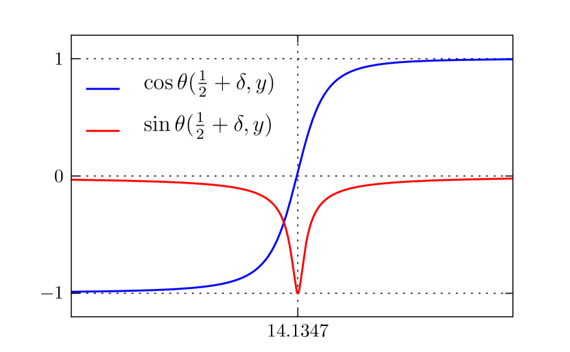
(a)

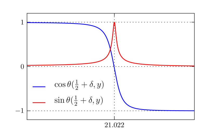
(b)

Figure 1: Exactly on a zero we have $\cos\theta=0$ and $\sin\theta=\pm 1$. This is illustrated for the first (a) and second (b) Riemann zeros, respectively. We plot $\cos\theta\left(\tfrac{1}{2}+\delta,y\right)$ and $\sin\theta\left(\tfrac{1}{2}+\delta,y\right)$ versus $y$, for $0<\delta\ll 1$.

Remark 2.

On the critical line, but not on a Riemann zero, $\theta=n\pi$ since $\chi=Ae^{i\theta}$ is real. Then $\cos\theta=\pm 1$ and $\sin\theta=0$. This shows that $\cos\theta$ alternates in sign around a zero, being a discontinuous function. The $\delta\to 0^{+}$ limit smooths out this discontinuity so we can define $\cos\theta=0$ exactly on a zero $z=\rho$, where we also have $\sin\theta=\pm 1$. This can be confirmed numerically as illustrated in FIG. 1 for the first two zeros.

Remark 3.

It is possible to introduce a new function $\zeta(z)\mapsto\widetilde{\zeta}(z)=f(z)\zeta(z)$ that also satisfies the functional equation (4), i.e. $\widetilde{\chi}(z)=\widetilde{\chi}(1-z)$, but has zeros off the critical line due to the zeros of $f(z)$. In such a case the corresponding functional equation will hold if and only if $f(z)=f(1-z)$ for any $z$, and this is a trivial condition on $f(z)$, which could have been canceled in the first place. Moreover, if $f(z)$ and $\zeta(z)$ have different zeros, the analog of equation (10) has a factor $f(z)$, i.e. $\widetilde{\chi}(\rho+\delta)+\widetilde{\chi}(1-\rho-\delta)=f(\rho+\delta)\left[\chi(\rho+\delta)+\chi(1-\rho-\delta)\right]=0$, implying (10) again where $\chi(z)$ is the original (3). Therefore, the previous analysis eliminates $f(z)$ automatically and only finds the zeros of $\chi(z)$. The analysis is non-trivial precisely because $\zeta(z)$ satisfies the functional equation but $\zeta(z)\neq\zeta(1-z)$. Furthermore, it is a well known theorem that the only function which satisfies the functional equation (4) and has the same characteristics of $\zeta(z)$, is $\zeta(z)$ itself. In other words, if $\widetilde{\zeta}(z)$ is required to have the same properties of $\zeta(z)$, then $\widetilde{\zeta}(z)=C\,\zeta(z)$, where $C$ is a constant (Titchmarsh, , pg. 31).

Remark 4.

Although equations (20) and (2) have an obvious resemblance, it is impossible to derive the former from the later, since the later is just a counting formula valid on the entire strip, and it is assumed that $T$ is not the ordinate of a zero. Moreover, this would require the assumption of the validity of the RH, contrary to our approach, where we derived equations (20) and (14) on the critical line, without assuming the RH. Despite our best efforts, we were not able to find formula (14) in the literature. The formula (15) has never been proven on the critical line Edwards . The current best estimate for the number of zeros on the critical line is given by $N_{0}(T)\geq\tfrac{2}{5}\,N(T)$ Conrey2 .

Remark 5.

One may object that our basic equation (14) involves $\zeta(z)$ itself and this is somehow circular. This is not a valid counter-argument. First of all, $\arg\zeta$ already appears in the counting function $N(T)$. Secondly, the equation (14) is a much more detailed equation than simply $\zeta(z)=0$, which has an infinite number of solutions, in contrast with (14) which for each $n$ has a unique solution corresponding to the $n$-th zero. Also, there are well-known ways to calculate the $\arg\zeta$ term, for example from an integral representation or a convergent series Borwein .

Remark 6.

The small shift by $\delta$ in (14) is essential since it smooths out $S(y)=\tfrac{1}{\pi}\arg\zeta\left(\tfrac{1}{2}+iy\right)$, which is known to jump discontinuously at each zero. As well known, $\arg\zeta\left(\tfrac{1}{2}+iy\right)$ is a piecewise continuous function, but rapidly oscillates around zero with discontinuous jumps, as shown in FIG. 2a. However, when this term is added to the smooth part of $N(T)$, one obtains an accurate staircase function, which jumps by one at each zero on the line; see FIG. 2b. In this form, the formula (15) counts the zeros on the critical line accurately, i.e. it does not miss any zero. Thus, as previously stated, since the Riemann-von Mangoldt function $N(T)$ has only been derived on the entire strip, and we have derived it for the zeros on the critical line, this indicates that all zeros are on the line.

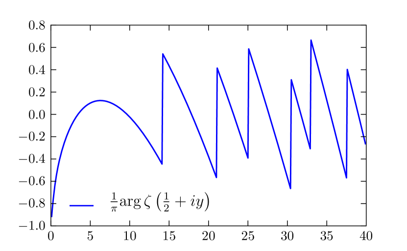
(a)

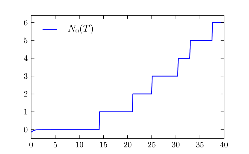
(b)

Figure 2: (a) A plot of $S(y)=\tfrac{1}{\pi}\arg\zeta\left(\tfrac{1}{2}+iy\right)$ as a function of $y$ showing its rapid oscillation. The jumps occur on a Riemann zero. (b) The function $N_{0}(T)$ in (15), which is indistinguishable from a manual counting of zeros.

III Approximate solution in terms of the Lambert function

III.1 Main formula

Let us now show that if one neglects the $\arg\zeta$ term, the equation (14) can be exactly solved. First, let us introduce the Lambert $W$ function Corless , which is defined for any complex number $z$ through the equation

$$W(z)e^{W(z)}=z.$$ (23)

The multi-valued $W$ function cannot be expressed in terms of other known elementary functions. If we restrict attention to real-valued $W(x)$ there are two branches. The principal branch occurs when $W(x)\geq-1$ and is denoted by $W_{0}$, or simply $W$ for short, and its domain is $x\geq-1/e$. The secondary branch, denoted by $W_{-1}$, satisfies $W_{-1}(x)\leq-1$ for $-e^{-1}\leq x<0$. Since we are interested in positive real-valued solutions of (14), we just need the principal branch where $W$ is single-valued.

Let us consider the leading order approximation of (14), or equivalently, its average since $\langle\arg\zeta\left(\tfrac{1}{2}+iy\right)\rangle=0$. Then we have the transcendental equation

$$\dfrac{\widetilde{y}_{n}}{2\pi}\log\left(\dfrac{\widetilde{y}_{n}}{2\pi e}\right)=n-\dfrac{11}{8}.$$ (24)

Through the transformation $\widetilde{y}_{n}=2\pi\left(n-\tfrac{11}{8}\right)x_{n}^{-1}$, this equation can be written as $x_{n}e^{x_{n}}=e^{-1}\left(n-\tfrac{11}{8}\right)$. Comparing with (23) its solution is given by $x_{n}=W\left[e^{-1}\left(n-\tfrac{11}{8}\right)\right]$, and thus we obtain

$$\widetilde{y}_{n}=\dfrac{2\pi\left(n-\tfrac{11}{8}\right)}{W\left[e^{-1}\left(n-\tfrac{11}{8}\right)\right]}.$$ (25)

Although the inversion from (24) to (25) is rather simple, it is very convenient since it is indeed an explicit formula depending only on $n$, and $W$ is included in most numerical packages. It gives an approximate solution for the ordinates of the Riemann zeros in closed form. The values computed from (25) are much closer to the Riemann zeros than Gram points, and one does not have to deal with violations of Gram’s law (see below).

III.2 Further remarks

Remark 7.

The estimates given by (25) can be calculated to high accuracy for arbitrarily large $n$, since $W$ is a standard elementary function. Of course, the $\widetilde{y}_{n}$ are not as accurate as the solutions $y_{n}$ including the $\arg\zeta$ term, as we will see in section IV. Nevertheless, it is indeed a good estimate, especially if one considers very high zeros, where traditional methods have not previously estimated such high values. For instance, formula (25) can easily estimate the zeros shown in TABLE 1, and much higher if desirable. The numbers in this table are accurate approximations to the $n$-th zero to the number of digits shown, which is approximately the number of digits in the integer part. For instance, the approximation to the $10^{100}$ zero is correct to $100$ digits. With Mathematica we easily calculated the first million digits of the $10^{10^{6}}$ zero.

$n$	$\widetilde{y}_{n}$
$10^{22}+1$	$1.370919909931995308226770\times 10^{21}$
$10^{50}$	$5.741532903784313725642221053588442131126693322343461\times 10^{48}$
$10^{100}$	$2.80690383842894069903195445838256400084548030162846045192360059224930$
	$922349073043060335653109252473234\times 10^{98}$
$10^{200}$	$1.38579222214678934084546680546715919012340245153870708183286835248393$
	$8909689796343076797639408172610028651791994879400728026863298840958091$
	$288304951600695814960962282888090054696215023267048447330585768\times 10^{198}$

Table 1: Formula (25) can easily estimate very high Riemann zeros. The results are expected to be correct up to the decimal point, i.e. to the number of digits in the integer part. The numbers are shown with three digits beyond the integer part.

Remark 8.

Using the asymptotic behaviour $W(x)\sim\log x$ for large $x$, the $n$-th zero is approximately $\widetilde{y}_{n}\approx 2\pi n/\log n$, as already known Titchmarsh . The distance between consecutive zeros is $2\pi/\log n$, which tends to zero when $n\to\infty$.

Remark 9.

The solutions $\widetilde{y}_{n}$ to the equation (24) are reminiscent of the so-called Gram points $g_{n}$, which are solutions to $\vartheta(g_{n})=n\pi$ where $\vartheta$ is given by (19). Gram’s law is the tendency for Riemann zeros to lie between consecutive Gram points, but it is known to fail for about $1/4$ of all Gram intervals. Our $\widetilde{y}_{n}$ are intrinsically different from Gram points, being an approximation to the ordinate of the $n$-th Riemann zero. In particular, the Gram point $g_{0}=17.8455$ is the closest to the first Riemann zero, whereas, $\widetilde{y}_{1}=14.52$ is much closer to the true zero which is $y_{1}\simeq 14.1347$. The traditional method to compute the zeros is based on the Riemann-Siegel formula, $\zeta\left(\tfrac{1}{2}+it\right)=Z(t)\left(\cos\vartheta(t)-i\sin\vartheta(t)\right)$, and the empirical observation that the real part of this equation is almost always positive, except when Gram’s law fails, and $Z(t)$ has the opposite sign of $\sin\vartheta$. Since $Z(t)$ and $\zeta\left(\tfrac{1}{2}+it\right)$ have the same zeros, one looks for the zeros of $Z(t)$ between two Gram points, as long as Gram’s law holds $(-1)^{n}Z\left(g_{n}\right)>0$. To verify the RH numerically, the counting formula (2) must also be used, to assure that the number of zeros on the critical line coincide with the number of zeros on the strip. The detailed procedure is throughly explained in Edwards ; Titchmarsh . Based on this method, amazingly accurate solutions and high zeros on the critical line were computed OdlyzkoSchonhage ; Odlyzko ; Odlyzko2 ; Gourdon . Nevertheless, our proposal is fundamentally different. We claim that (20), or its asymptotic approximation (14), is the equation that determines the Riemann zeros on the critical line. Then, one just needs to find its solution for a given $n$. We will compute the Riemann zeros in this way in the next section, just by solving the equation numerically, starting from the approximation given by the explicit formula (25), without using Gram points nor the Riemann-Siegel $Z$ function. Let us emphasize that our goal is not to provide a more efficient algorithm to compute the zeros OdlyzkoSchonhage , although the method described here may very well be, but to justify the validity of equations (14) and (20).

IV Numerical solutions

Instead of solving the exact equation (20) we will initially consider its first order approximation, which is equation (14). As we will see, this approximation already yields surprisingly accurate values for the Riemann zeros.

Let us first consider how the approximate solution given by (25) is modified by the presence of the $\arg\zeta$ term in (14). Numerically, we compute $\arg\zeta$ taking its principal value. As already discussed in Remark 6, the function $\arg\zeta\left(\tfrac{1}{2}+iy\right)$ oscillates around zero and changes sign in the vicinity of each Riemann zero, as shown in FIG. 2a. At a zero it can be well-defined by the limit (8), which is generally not zero. For example, for the first Riemann zero $y_{1}\simeq 14.1347$, $\lim_{\delta\to 0^{+}}\arg\zeta\left(\tfrac{1}{2}+\delta+iy_{1}\right)=0.1578739$. The $\arg\zeta$ term plays an important role and indeed improves the estimate of the $n$-th zero. This can be seen from FIG. 3a for a randomly chosen $n$. It practically cancels (24) around the zero, and exactly at the true zero we have a jump. The value predicted by (25) is then slightly changed. For a given $n$, the problem of finding the value $y_{n}$ where this jump occurs, yields the $n$-th Riemann zero as the numerical solution of (14).

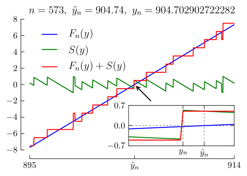
(a)

(b)

Figure 3: (a) Graph of the different terms present in equation (14). Here we have $F_{n}(y)=\tfrac{y}{2\pi}\log\left(\tfrac{y}{2\pi e}\right)-n+\tfrac{11}{8}$, equation (24), and $S(y)=\tfrac{1}{\pi}\arg\zeta\left(\tfrac{1}{2}+iy\right)$. $F_{n}(y)+S(y)$ is the complete equation (14). Note how $\widetilde{y}_{n}$ is dislocated by the $\arg\zeta$ term, yielding a much more precise result. (b) Comparison of the prediction of (25) (blue line) and (14) (red dots). The numerical solutions of (14) oscillate around the line predicted by (25) due to the fluctuating term $\arg\zeta$.

Since equation (14) alternates in sign around a zero, it is convenient to use Brent’s method BrentMethod to find its root. We applied this method, looking for a root in an appropriate interval, centered around the approximate solution $\widetilde{y}_{n}$ given by formula (25). Some of the solutions are presented in TABLE 2, and are accurate up to the number of decimal places shown. We used only Mathematica or some very simple algorithms to perform these numerical computations, taken from standard open source numerical libraries. We present the numbers accurate up to $9$ digits after the integer part.

$n$	$\widetilde{y}_{n}$	$y_{n}$
$1$	$14.52$	$14.134725142$
$10$	$50.23$	$49.773832478$
$10^{2}$	$235.99$	$236.524229666$
$10^{3}$	$1419.52$	$1419.422480946$
$10^{4}$	$9877.63$	$9877.782654006$
$10^{5}$	$74920.89$	$74920.827498994$
$10^{6}$	$600269.64$	$600269.677012445$
$10^{7}$	$4992381.11$	$4992381.014003180$
$10^{8}$	$42653549.77$	$42653549.760951554$
$10^{9}$	$371870204.05$	$371870203.837028053$
$10^{10}$	$3293531632.26$	$3293531632.397136704$

Table 2: Numerical solutions of equation (14). All numbers shown are accurate up to the $9$-th decimal place, in comparison with Odlyzko ; Oliveira .

$n$	$y_{n}$
$1$	$14.13472514173469379045725198356247$
$2$	$21.02203963877155499262847959389690$
$3$	$25.01085758014568876321379099256282$
$4$	$30.42487612585951321031189753058409$
$5$	$32.93506158773918969066236896407490$

Table 3: Numerical solutions to (14) for the lowest zeros. Although it was derived for high $y$, it provides accurate numbers even for the lower zeros. This numbers are correct up to the decimal place shown Odlyzko .

Although the formula for $y_{n}$ was derived for large $y$, it is surprisingly accurate even for the lower zeros, as shown in TABLE 3. It is actually easier to solve numerically for low zeros since $\arg\zeta$ is better behaved. These numbers are correct up to the number of digits shown, and the precision was improved simply by decreasing the error tolerance.

Riemann zeros have previously been calculated to high accuracy using sophisticated algorithms OdlyzkoSchonhage , which are not based on solving our equation (14). Nevertheless, we have verified that (14) is well satisfied to the degree of accuracy of these zeros. This can be seen in TABLE 4 where we show the absolute value of (14), replaced with our numerical solutions, and its value calculated with much more accurate Riemann zeros, up to the $150$-th decimal place, provided by Mathematica.

$n$	$|\mbox{\eqref{FinalTranscendence}}|$	$|\mbox{\eqref{FinalTranscendence}}|$
$1$	$0.082$	$0.00047$
$2$	$0.071$	$0.00032$
$3$	$0.046$	$0.00026$
$4$	$0.044$	$0.00022$
$5$	$0.081$	$0.00020$

$n$	$|\mbox{\eqref{FinalTranscendence}}|$	$|\mbox{\eqref{FinalTranscendence}}|$
$10^{5}-4$	$0.10$	$0.000000088$
$10^{5}-3$	$0.094$	$0.000000089$
$10^{5}-2$	$0.072$	$0.000000090$
$10^{5}-1$	$0.034$	$0.000000088$
$10^{5}$	$0.059$	$0.000000089$

Table 4: We substitute numerical solutions of $y_{n}$ into equation (14). The values $|(\ref{FinalTranscendence})|$ denote the absolute value of the difference between the RHS and LHS of the equation. We use $\delta=10^{-9}$. The second column is the value obtained with our solutions, accurate to 9 decimal places. The third column is the value obtained with solutions accurate up to 150 decimal places, computed through another algorithm, which is not based on solving (14). This shows that (14) is indeed satisfied for high accurate Riemann zeros.

V GUE Statistics

The link between the Riemann zeros and random matrix theory started with the pair correlation of zeros, proposed by Montgomery Montgomery , and the observation of F. Dyson that it is the same as the 2-point correlation function predicted by the gaussian unitary ensemble (GUE) for large random matrices Dyson .

The main purpose of this section is to test whether our approximation (14) to the zeros is accurate enough to reveal this statistics. Whereas formula (25) is a valid estimate of the zeros, it is not sufficiently accurate to reproduce the GUE statistics, since it does not have the oscillatory $\arg\zeta$ term. On the other hand, the solutions to equation (14) are accurate enough, which indicates the importance of the $\arg\zeta$.

Montgomery’s pair correlation conjecture can be stated as follows:

$$\dfrac{1}{N(T)}\sum_{\begin{subarray}{c}0\leq y,y^{\prime}\leq T\\[2.79996pt] \alpha<\tfrac{1}{2\pi}\log\left(\tfrac{T}{2\pi}\right)\left(y-y^{\prime}\right)\leq\beta\end{subarray}}1\quad\sim\quad\int_{\alpha}^{\beta}du\left(1-\dfrac{\sin^{2}\left(\pi u\right)}{\pi^{2}u^{2}}\right)$$ (26)

where $0<\alpha<\beta$, $N(T)\sim\tfrac{T}{2\pi}\log\left(\tfrac{T}{2\pi}\right)$ according to (15), and the statement is valid in the limit $T\to\infty$. The right hand side of (26) is the 2-point GUE correlation function. The average spacing between consecutive zeros is given by $\tfrac{T}{N}\sim 2\pi/\log\left(\tfrac{T}{2\pi}\right)\to 0$ as $T\to\infty$. This can also be seen from (25) for very large $n$, i.e. $\widetilde{y}_{n+1}-\widetilde{y}_{n}\to 0$ as $n\to\infty$. Thus the distance between zeros on the left hand side of (26), under the sum, is a normalized distance.

While (26) can be applied if we start from the first zero on the critical line, it is unable to provide a test if we are centered around a given high zero on the line. To deal with such a situation, Odlyzko Odlyzko2 proposed a stronger version of Montgomery’s conjecture, by taking into account the large density of zeros higher on the line. This is done by replacing the normalized distance in (26) by a sum of normalized distances over consecutive zeros in the form

$$\delta_{n}\equiv\dfrac{1}{2\pi}\log\left(\dfrac{y_{n}}{2\pi}\right)\left(y_{n+1}-y_{n}\right).$$ (27)

Thus (26) is replaced by

$$\dfrac{1}{\left(N-M\right)\left(\beta-\alpha\right)}\sum_{\begin{subarray}{c}M\leq m,n\leq N\\[2.79996pt] \alpha<\sum_{k=1}^{n}\delta_{m+k}\leq\beta\end{subarray}}1\quad=\quad\dfrac{1}{\beta-\alpha}\int_{\alpha}^{\beta}du\left(1-\dfrac{\sin^{2}\left(\pi u\right)}{\pi^{2}u^{2}}\right),$$ (28)

where $M$ is the label of a given zero on the line and $N>M$. In this sum it is assumed that $n>m$ also, and we included the correct normalization on both sides. The conjecture (28) is already well supported by extensive numerical analysis Odlyzko2 ; Gourdon .

Odlyzko’s conjecture (28) is a very strong constraint on the statistics of the zeros. Thus we submit the numerical solutions of equation (14), as discussed in the previous section, to this test. In FIG. 4a we can see the result for $M=1$ and $N=10^{5}$, with $\alpha$ ranging from $0\dotsc 3$ in steps of $s=0.05$, and $\beta=\alpha+s$ for each value of $\alpha$, i.e. $\alpha=[0.00,\,0.05,\,0.10,\dotsc,\,3.00]$ and $\beta=[0.05,\,0.10,\,\dotsc,\,3.05]$. We compute the left hand side of (28) for each pair $(\alpha,\beta)$ and plot the result against $x=\tfrac{1}{2}\left(\alpha+\beta\right)$. In FIG. 4b we do the same thing but with $M=10^{9}-10^{5}$ and $N=10^{9}$. Clearly, the numerical solutions of (14) reproduce the correct statistics. In fact, FIG. 4a is identical to the one in Odlyzko2 . The last zeros in these ranges are shown in TABLE 5.

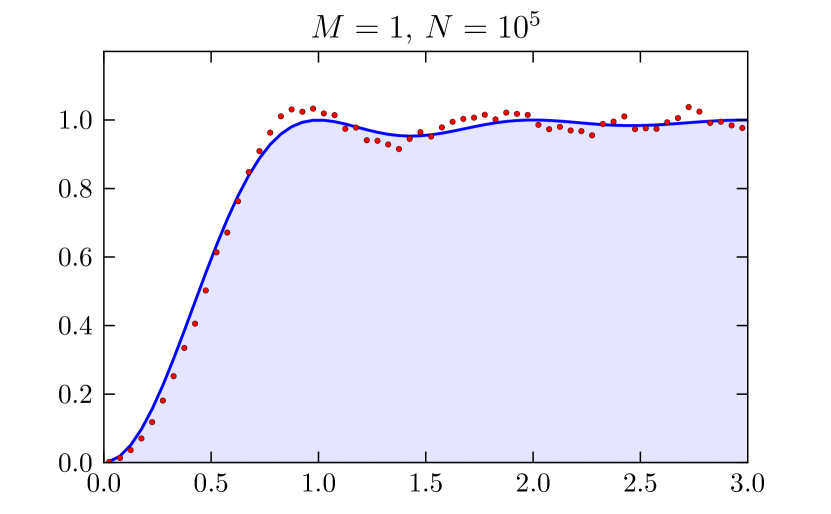
(a)

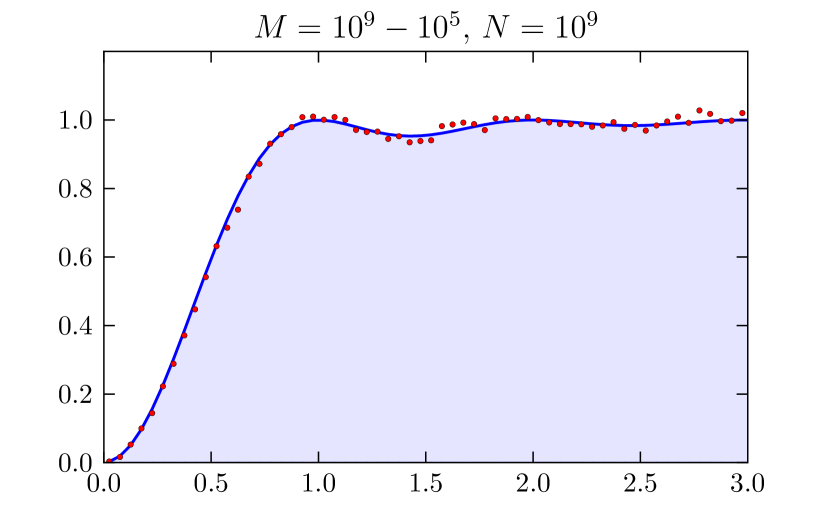
(b)

Figure 4: (a) The solid line represents the RHS of (28) and the dots represent its LHS, computed from the numerical solutions of equation (14). The parameters are $\beta=\alpha+0.05$, $\alpha=[0,\,0.05,\,\dotsc,\,3]$ and the $x$-axis is given by $x=\tfrac{1}{2}\left(\alpha+\beta\right)$. We use the first $10^{5}$ zeros. (b) The same parameters but using zeros in the middle of the critical line, i.e. $M=10^{9}-10^{5}$ and $N=10^{9}$.

$n$	$y_{n}$
$10^{5}-5$	$74917.719415828$
$10^{5}-4$	$74918.370580227$
$10^{5}-3$	$74918.691433454$
$10^{5}-2$	$74919.075161121$
$10^{5}-1$	$74920.259793259$
$10^{5}$	$74920.827498994$

$n$	$y_{n}$
$10^{9}-5$	$371870202.244870424$
$10^{9}-4$	$371870202.673284411$
$10^{9}-3$	$371870203.177729726$
$10^{9}-2$	$371870203.274345875$
$10^{9}-1$	$371870203.802552402$
$10^{9}$	$371870203.837028146$

Table 5: Last numerical solutions to (14) around $n=10^{5}$ and $n=10^{9}$. In the first table the solutions are accurate up to the $8$-th decimal place, while in the second table up to the $6$-th decimal place Odlyzko ; Oliveira .

VI Prime number counting function

In this section we explore whether our approximations to the Riemann zeros are accurate enough to reconstruct the prime number counting function. As usual, let $\pi(x)$ denote the number of primes less than $x$. Riemann obtained an explicit expression for $\pi(x)$ in terms of the non-trivial zeros of $\zeta(z)$. There are simpler but equivalent versions of the main result, based on the function $\psi(x)$ below. However, let us present the main formula for $\pi(x)$ itself, since it is historically more important.

The function $\pi(x)$ is related to another number-theoretic function $J(x)$, defined as

$$J(x)=\sum_{2\leq n\leq x}\dfrac{\Lambda(n)}{\log n}$$ (29)

where $\Lambda(n)$, the von Mangoldt function, is equal to $\log p$ if $n=p^{m}$ for some prime $p$ and an integer $m$, and zero otherwise. The two functions $\pi(x)$ and $J(x)$ are related by Möbius inversion:

$$\pi(x)=\sum_{n\geq 1}\dfrac{\mu(n)}{n}J(x^{1/n}).$$ (30)

Here, $\mu(n)$ is the Möbius function, equal to $1$ ($-1$) if $n$ is a product of an even (odd) number of distinct primes, and equal to zero if it has a multiple prime factor. The above expression is actually a finite sum, since for large enough $n$, $x^{1/n}<2$ and $J=0$.

The main result of Riemann is a formula for $J(x)$, expressed as an infinite sum over zeros $\rho$ of the $\zeta(z)$ function:

$$J(x)={\rm Li}(x)-\sum_{\rho}{\rm Li}\left(x^{\rho}\right)+\int_{x}^{\infty}\dfrac{dt}{\log t}~{}\dfrac{1}{t\left(t^{2}-1\right)}-\log 2,$$ (31)

where ${\rm Li}(x)=\int_{0}^{x}dt/\log t$ is the log-integral function . The above sum is real because the $\rho$’s come in conjugate pairs. If there are no zeros on the line $\Re(z)=1$, then the dominant term is the first one in the above equation, $J(x)\sim{\rm Li}(x)$, and this was used to prove the prime number theorem by Hadamard and de la Vallée Poussin.

The function $\psi(x)$ has the simpler form

$$\psi(x)=\sum_{n\leq x}\Lambda(n)=x-\sum_{\rho}\dfrac{x^{\rho}}{\rho}-\log(2\pi)-\dfrac{1}{2}\log\left(1-\dfrac{1}{x^{2}}\right).$$ (32)

In this formulation, the prime number theorem follows from the fact that the leading term is $\psi(x)\sim x$.

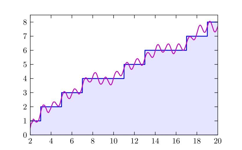
(a)

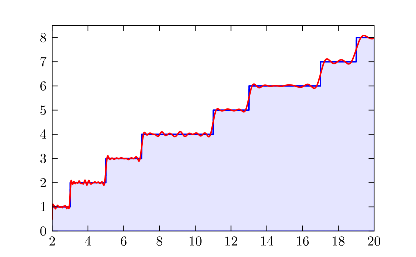
(b)

Figure 5: (a) The prime number counting function $\pi(x)$ with the first $50$ Riemann zeros approximated by the formula (25). (b) The same plot but with the first $50$ Riemann zeros approximated by numerical solutions to the equation (14).

In Figure FIG. 5a we plot $\pi(x)$ from equations (30) and (31), computed with the first $50$ zeros in the approximation $\rho_{n}=\tfrac{1}{2}+i\widetilde{y}_{n}$ given by (25). FIG. 5b shows the same plot with zeros obtained from the numerical solution of equation (14). Although with the approximation $\widetilde{y}_{n}$ the curve is trying to follow the steps in $\pi(x)$, once again, one clearly sees the importance of the $\arg\zeta$ term.

VII Numerical solutions to the exact equation

In the previous sections we have computed numerical solutions of (14) showing that, actually, this first order approximation to (20) is very good and already captures the interesting properties of the Riemann zeros, like the GUE statistics and ability to reproduce the prime number counting formula. Nevertheless, by simply solving (20) it is possible to obtain values for the zeros as accurately as desirable. The numerical procedure is performed as follows:

1. We solve (20) looking for the solution in a region centered around the number $\widetilde{y}_{n}$ provided by (25), with a not so small $\delta$, for instance $\delta\sim 10^{-5}$.

2. We solve (20) again but now centered around the solution obtained in step 1 above, and we decrease $\delta$, for instance $\delta\sim 10^{-8}$.

3. We repeat the procedure in step 2 above, decreasing $\delta$ again.

4. Through successive iterations, and decreasing $\delta$ each time, it is possible to obtain solutions as accurate as desirable. In carrying this out, it is important to not allow $\delta$ to be exactly zero.

The first few zeros are shown in TABLE 6. We simply applied the standard root finder in Mathematica . Through successive iterations it is possible achieve even much higher accuracy than shown in TABLE 6.

$n$	$y_{n}$
$1$	$14.1347251417346937904572519835624702707842571156992431756855$
$2$	$21.0220396387715549926284795938969027773343405249027817546295$
$3$	$25.0108575801456887632137909925628218186595496725579966724965$
$4$	$30.4248761258595132103118975305840913201815600237154401809621$
$5$	$32.9350615877391896906623689640749034888127156035170390092800$

Table 6: The first few numerical solutions to (20), accurate to $60$ digits ($58$ decimals). These solutions were obtained using the root finder function in Mathematica.

It is known that the first zero where Gram’s law fails is for $n=126$. Applying the same method, like for any other $n$, the solution of (20) starting with the approximation (25) does not present any difficulty. We easily found the following number:

$$279.229250927745189228409880451955359283492637405561293594727\qquad(n=126)$$

Just to illustrate, and to convince the reader, how the solutions of (20) can be made arbitrarily precise, we compute the zero $n=1000$ accurate up to $500$ decimal places, also using the same simple approach :

$$1419. 42248094599568646598903807991681923210060106416601630469081468460$$

$$8676417593010417911343291179209987480984232260560118741397447952650637$$

$$0672508342889831518454476882525931159442394251954846877081639462563323$$

$$8145779152841855934315118793290577642799801273605240944611733704181896$$

$$2494747459675690479839876840142804973590017354741319116293486589463954$$

$$5423132081056990198071939175430299848814901931936718231264204272763589$$

$$1148784832999646735616085843651542517182417956641495352443292193649483$$

$$857772253460088$$

Substituting precise Riemann zeros calculated by other means Odlyzko into (20) one can check that the equation is identically satisfied. These results corroborate that (20) is an exact equation for the Riemann zeros, which was derived on the critical line.

VIII Final remarks

Let us summarize our main results and arguments. Throughout this paper we did not assume the Riemann hypothesis. The main outcome was the demonstration that there are infinite zeros on the critical line, $\rho_{n}=\tfrac{1}{2}+iy_{n}$, where $y_{n}$ exactly satisfies the equation (20). Asymptotically this equation can be approximated by (14). Furthermore, we argued that these equations can be made continuous through the $\delta\to 0^{+}$ limit, and therefore, they should have a unique solution for every single $n$. Under this assumption, the number of solutions on the critical line already saturates the counting formula for the number of zeros on the entire critical strip. This is a strong indication that (20) captures all non-trivial zeros, which must therefore be all on the critical line. Although our approach cannot be considered as a rigorous proof, it is at the very least a clear strategy towards proving the Riemann hypothesis. It is important to note that (20) and (14) were derived on the critical line, while the counting formulas (2) and (1) can only be derived on the entire strip. Thus it is impossible to obtain the former from the latter without assuming the Riemann hypothesis.

We verified numerically that the simplest approximation to the exact equation (20), namely (14), is enough to capture the statistical properties of the Riemann zeros. We did so by testing the Montgomery-Odlyzko pair correlation conjecture, and by reconstructing the prime number counting function, employing the numerical solutions of equation (14). In solving such transcendental equation, we started from an approximate solution given by the explicit formula (25). Thus, we did not require the use of Gram points and we also did not have to deal with violations of Gram’s law. We also computed some numerical solutions of the exact equation (20), which proved to be much more stable under the numerical approach. This procedure constitutes a novel method to compute the zeros. Therefore, the numerical results strongly support the validity of our assertions, claiming that (20) is an exact equation, identically satisfied by the $n$-th Riemann zero on the critical line.

We also wish to mention that we have extended this work to two infinite classes of $L$-functions, those based on Dirichlet characters and modular forms Lfunctions .

References

- (1) H. M. Edwards, Riemann’s Zeta Function, Dover Publications Inc., 1974.
- (2) P. Sarnak, Problems of the Millennium: The Riemann hypothesis, Clay Mathematics Institute (2004).
- (3) E. Bombieri, Problems of the Millennium: The Riemann hypothesis, Clay Mathematics Institute (2000).
- (4) J. B. Conrey, The Riemann Hypothesis, Notices of the AMS 50 (2003) 342.
- (5) E. C. Titchmarsh, The Theory of the Riemann Zeta-Function, Oxford University Press, 1988.
- (6) N. Levinson, More than one third of the zeros of Riemann’s zeta-function are on , Advances in Math. 13 (1974) 383–436.
- (7) J. B. Conrey, More than two fifths of the zeros of the Riemann zeta function are on the critical line, J. reine angew. Math. 399 (1989) 1–26.
- (8) H. Montgomery, The pair correlation of zeros of the zeta function, Analytic number theory, Proc. Sympos. Pure Math. XXIV, Providence, R.I.: AMS, pp. 181D193, 1973.
- (9) M. V. Berry, Riemann’s Zeta Function: A Model for Quantum Chaos?, Quantum Chaos and Statistical Nuclear Physics, Eds. T. H. Seligman and H. Nishioka, Lecture Notes in Physics, 263 Springer Verlag, New York, 1986.
- (10) M. V. Berry and J. P. Keating, The Riemann zeros and eigenvalue asymptotics, SIAM Review 41 (1999) 236.
- (11) M. V. Berry and J. P. Keating, and the Riemann zeros, in Supersymmetry and Trace Formulae: Chaos and Disorder, Kluwer 1999.
- (12) G. Sierra, The Riemann zeros and the cyclic Renormalization Group, J. Stat. Mech. 0512:P12006 (2005).
- (13) G. Sierra, A Quantum Mechanical model of the Riemann Zeros, New J. Phys. 10 (2008) 033016.
- (14) R. K. Baduri, A. Khare and J. Law, The Phase of the Riemann Zeta Function and the Inverted Harmonic Oscillator, Phys. Rev. E52 (1995) 486.
- (15) A. Connes, Trace formula in noncommutative geometry and the zeros of the Riemann zeta function, Sel. Math. New Ser. 5 (1999) 29–106.
- (16) J.-B. Bost and A. Connes Hecke algebras, type III factors and phase transitions with spontaneos symmetry breaking in number theory, Sel. Math. New Ser. 3 (1995) 411–457.
- (17) D. Schumayer and D. A. W. Hutchinson, Physics of the Riemann hypothesis, Rev. Mod. Phys. 83 (2011) 307–330.
- (18) J. van de Lune, H. J. J. te Riele and D. T. Winter, On the zeros of the Riemann zeta function in the critical strip. IV, Math. Comp. 46 (1986) 667–681.
- (19) X. Gourdon, The first zeros of the Riemann Zeta function, and zeros computation at very large height (2004).
- (20) A. LeClair, An electrostatic depiction of the validity of the Riemann Hypothesis and a formula for the -th zero at large , Int. J. Mod. Phys. A 28 (2013) 1350151, arXiv:1305.2613 [math-ph].
-
(21)
A. Odlyzko,
Tables of zeros of the Riemann zeta function,
www.dtc.umn.edu/ odlyzko/zeta-tables/. - (22) A. LeClair, Interacting Bose and Fermi gases in low dimensions and the Riemann Hypothesis, Int. J. Mod. Phys. A 23 (2008) 1371, arXiv:math-ph/0611043.
- (23) D. A. Goldston and S. M. Gonek, A note on and the zeros of the Riemann zeta-function, Bull. London Math. Soc. 39 (2007) 482–486.
- (24) J. M. Borwein, D. M. Bradley and R. E. Crandall, Computational strategies for the Riemann zeta function, J. Comp. and App. Math. 121 (200) 247–296.
- (25) R. M. Corless, G. H. Gonnet, D. E. G. Hare, D. J. Jeffrey, and D. E. Knuth, Adv. Comp. Math. 5 (1996) 329–359.
- (26) W. H. Press, S. A. Teukolsky, W. T. Vetterling and B. P. Flannery, Numerical Recipes in C, Cambridge University Press, 1992, pp. 359.
-
(27)
T. Oliveira e Silva,
Tables of zeros of the Riemann zeta function, (2010)
http://sage.math.washington.edu/home/kstueve/L_functions/RiemannZetaFunction/. - (28) A. M. Odlyzko and A. Schönhage, Fast algorithms for multiple evaluations of the Riemann zeta function, Trans. Amer. Math. Soc. 309 (2) (1988): 797D809.
- (29) F. Dyson, Correlations between eigenvalues of a random matrix, Comm. Math. Phys. 19 (1970) 235.
- (30) A. M. Odlyzko, On the Distribution of Spacings Between Zeros of the Zeta Function, Math. of Computation 177 (1987) 273.
- (31) G. França and A. LeClair, On the zeros of L-functions, arXiv:1309.7019 [math.NT].