It takes a village to raise a tide: nonlinear multiple-mode coupling and mode identification in KOI-54

Abstract

We explore the tidal excitation of stellar modes in binary systems using Kepler observations of the remarkable eccentric binary KOI-54 (HD 187091; KIC 8112039), which displays strong ellipsoidal variation as well as a variety of linear and nonlinear pulsations. We report the amplitude and phase of over 120 harmonic and anharmonic pulsations in the system. We use pulsation phases to determine that the two largest-amplitude pulsations, the 90th and 91st harmonics, most likely correspond to axisymmetric $m=0$ modes in both stars, and thus cannot be responsible for resonance locks as had been recently proposed. We find evidence that the amplitude of at least one of these two pulsations is decreasing with a characteristic timescale of $\sim 100\,$yr. We also use the pulsations’ phases to confirm the onset of the traveling wave regime for harmonic pulsations with frequencies $\lesssim 50\;\Omega_{\rm orb}$, in agreement with theoretical expectations. We present evidence that many pulsations that are not harmonics of the orbital frequency correspond to modes undergoing simultaneous nonlinear coupling to multiple linearly driven parent modes. Since coupling among multiple modes can lower the threshold for nonlinear interactions, nonlinear phenomena may be easier to observe in highly eccentric systems, where broader arrays of driving frequencies are available. This may help to explain why the observed amplitudes of the linear pulsations are much smaller than the theoretical threshold for decay via three-mode coupling.

1 Introduction

Stars and planets in eccentric orbits exchange energy and angular momentum through tidal interactions. The net tidal fluid response can be conceptually divided into two components. The equilibrium tide is the large-scale prolate distortion caused by nonresonantly excited stellar modes (Zahn, 1977). The dynamical tide, which is our focus in this work, corresponds to low-frequency internal waves (gravity and inertial) that are resonantly excited by the time-varying tidal potential. Such waves have much shorter damping times, and are expected to play an important role in the circularization of orbits and spin up of stars (e.g., Zahn, 1975; Goldreich & Nicholson, 1989; Witte & Savonije, 2002). Although most prior work on tides has been calculated in the linear regime, nonlinear effects may play an important role in redistributing energy and angular momentum in binary systems on much shorter timescales (e.g., Barker & Ogilvie, 2010; Weinberg et al., 2012).

In this work, we explore the role of linear and nonlinear dynamical tides in the recently discovered Kepler system KOI-54 (HD 187091; KIC 8112039; Welsh et al. 2011, hereafter W11). In particular, we aim to understand the nature of the largest-amplitude tidally excited pulsations to ascertain if they are responsible for resonance locks, a phenomenon that allows for efficient spin-orbit coupling in binary systems (Witte & Savonije, 2002). More generally, we explore the harmonic and anharmonic pulsations that we observe in this particular binary system, and address how their amplitudes and frequencies are determined by a complex set of nonlinear interactions amongst many different modes.

Recently, Burkart et al. (2012, hereafter B12) developed a quantitative framework for analyzing such pulsations, which they termed tidal asteroseismology (see also Fuller & Lai 2012). This work used theoretical stellar models to investigate the linear, nonadiabatic response of stars to linearly excited resonant oscillations. This analysis naturally explained many qualitative features of KOI-54’s harmonic pulsations. Nonetheless, several puzzles remained.

One unresolved question was the nature of the two most prominent pulsations in the system, which have frequencies that are the 90th & 91st harmonics of the orbital frequency. The amplitudes of the pulsations ($294\,\mu$mag and $228\,\mu$mag, or parts-per-million, respectively) are considerably larger than any of the other pulsations; indeed, B12 estimated that the probability of their occurrence through purely linear excitation to be only $\sim 1\%$. Both Fuller & Lai (2012) and B12 considered the possibility that the two pulsations could be occurring due to two $l=2$, $|m|=2$ g-modes responsible for resonance locks. Fuller & Lai (2012) showed that the frequencies of the 90th and 91st harmonics are within a few percent of the natural, a priori prediction of the most likely frequency at which resonance locks should occur, given KOI-54’s observed system parameters. However, B12 found that the maximum torque possible from likely modes was much too small to effect a resonance lock, and also pointed out that it is unlikely for two resonance locks to occur simultaneously.

B12 and Fuller & Lai (2012) also reported that the two largest anharmonic pulsations appear to be driven by the parametric instability of the $91$st harmonic. However, B12 found that the estimated amplitude for a mode to become overstable and drive the parametric instability is $\sim 100\times$ larger than the observed amplitude of the $91$st harmonic if it is an $m=0$ mode.

We address the nature of the harmonic pulsations by analyzing their amplitudes and frequencies together with their phases. B12 (see also Willems, van Hoolst & Smeyers, 2003) showed that the observed phase of the pulsations depends on the excited mode’s azimuthal order $m$, its damping rate $\gamma$, and the difference $\delta\omega$ between the eigenmode frequency and the driving frequency (see eq. 2).

In this work, we extend the work of W11 using additional publicly available Kepler data to determine all of the observable properties of the pulsations, in particular their phases, which were not originally reported. This allows us to determine more information about the modes responsible for the individual pulsations, in particular the azimuthal order $m$. Furthermore, with the addition of five more quarters of data, and consequently greater signal-to-noise ratios, we are able to search for pulsations with amplitudes lower than W11 were able to detect.

The structure of our paper is as follows. We describe Kepler photometry and our data reduction routine in § 2, and give an overview of the observed pulsations in § 3. In § 4, we analyze the tidally driven, linear oscillations of KOI-54. In § 5, we analyze the nonlinear oscillations. Finally, we summarize our results and discuss their implications in § 6.

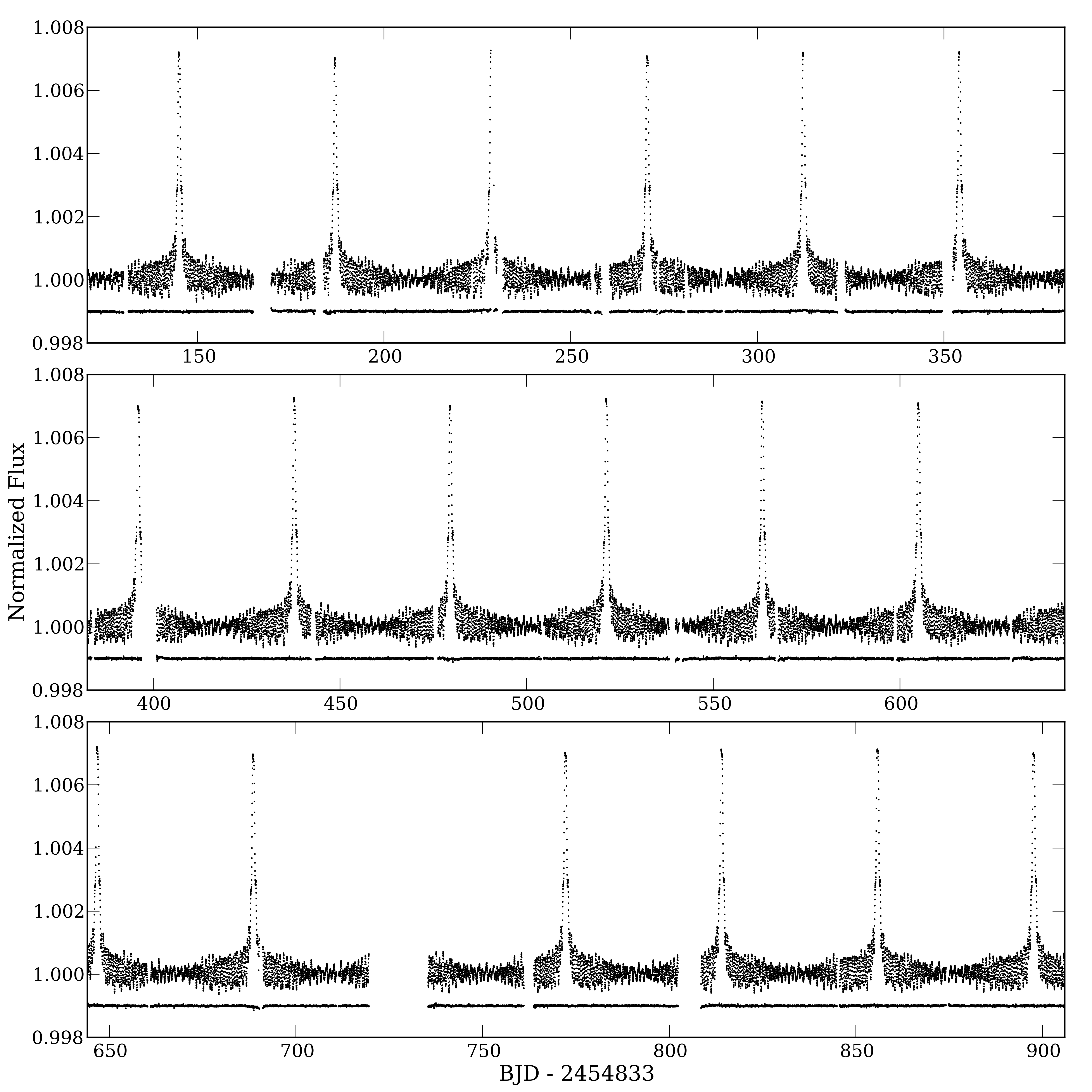
Figure 1: KOI-54 lightcurve. Plotted is the normalized flux of KOI-54 with the data detrended as in § 2. Below the lightcurve we show residuals from subtracting our ellipsoidal model and 182 of the best-fit sinusoidal pulsations.

2 Kepler photometry and detrending

We use 785.4 d of nearly continuous photometric observations of KOI-54 that have been publicly released by the Kepler mission (Borucki et al., 2010; Koch et al., 2010). During these observations, the satellite underwent multiple safe-mode shutdowns, as well as scheduled rollings that introduce large artifacts into the raw data. We detrend the data and remove these artifacts in the following way. We visually inspect the released raw data, and remove, by eye, obvious outliers due to cosmic rays. After inspection, we fit cubic polynomials (and lines) to each series of contiguous data simultaneously along with a photometric model for the periastron brightening events as well as 30 sinusoids for the largest-amplitude pulsations. We then remove all outliers that deviate from the remaining data by more than three standard deviations, and refit our models and detrending curves. After we detrend the data, we subsequently subtract the photometric model from the normalized lightcurve and remove low-frequency pulsations with a Hann window function of width $8\,$d.

W11 employed the proprietary ELC modeling code (Orosz & Hauschildt, 2000) to simultaneously fit the Kepler photometry together with complementary radial velocity observations of KOI-54. We instead use the much faster and simpler photometric model detailed in B12 (Appendix B), which is sufficient to determine the amplitudes, frequencies, and phases (and any variations) of the high-frequency ($f\gtrsim 20\Omega_{\rm orb}$) dynamical tide with minimal contamination from the equilibrium tide and stellar irradiation. This linear model decomposes the stellar flux perturbation induced by the equilibrium tide into spherical harmonics, making use of von Zeipel’s theorem (von Zeipel, 1924). The effects of irradiation of each star by its companion are also included, and are modeled as absorption and immediate reemission at the photosphere. We evaluate changes in luminosity due to the equilibrium tide and irradiation up to spherical harmonic degree $l=3$; higher-degree harmonics do not contribute significantly to the signal.

To model limb darkening, we use the four-coefficient nonlinear fit found in Howarth (2011) determined for the Kepler bandpass for an $8,800$ K star with a surface gravity $\log g=4$, consistent with best-fit parameters of both stars in W11. We then find the least-squares best fit for the orbital period, epoch of periastron, and bandpass correction coefficients $\beta_{1}$ & $\beta_{2}$. For the remaining parameters, we use the best-fit values in W11. In principle, it should be possible to determine $\beta_{1}$ and $\beta_{2}$ a priori, as was done in W11. We find that for the objectives of this paper, by fitting for $\beta_{1}$ and $\beta_{2}$ and subtracting the ellipsoidal variation and irradiation from the lightcurve, we do not introduce any significant errors in our assessment of the high-frequency pulsations. The parameters of KOI-54 used in this study are listed in Table 1.

Table 1: System parameters of KOI-54. From top to bottom are the derived properties of the binary from spectroscopic observations, best-fit system parameters from the photometric model of W11, best-fit parameters using our photometric model, and the tabulated coefficients used in the photometric model in this work.

	parameter	value	error	unit
Observations (W11)
	$T_{1}$	8500	200	K
	$T_{2}$	8800	200	K
	$L_{2}/L_{1}$	1.22	0.04
	$v_{\mathrm{rot},1}\sin{i_{1}}$	7.5	4.5	$\mathrm{km}/\mathrm{s}$
	$v_{\mathrm{rot},2}\sin{i_{2}}$	7.5	4.5	$\mathrm{km}/\mathrm{s}$
	$[\text{Fe}/\text{H}]_{1}$	0.4	0.2
	$[\text{Fe}/\text{H}]_{2}$	0.4	0.2
Lightcurve modeling (W11)
	$P_{\rm orb}$	41.8050	0.0003	days
	$T_{\rm p}$	2455103.5490	0.0010	BJD
	$e$	0.8335	0.0005
	$\omega$	36.70	0.90	degrees
	$i$	5.50	0.10	degrees
	$a$	0.3956	0.008	AU
	$M_{2}/M_{1}$	1.024	0.013
	$R_{1}$	2.20	0.03	${\rm R}_{\odot}$
	$R_{2}$	2.33	0.03	${\rm R}_{\odot}$
Lightcurve modeling (this work)
	$P_{\rm orb}$	41.8050	0.0001	days
	$T_{\rm p}$	2455061.73814	0.006	BJD
	$\beta(T_{1})$	0.489
	$\beta(T_{2})$	0.818
Limb darkening coefficients (Howarth 2011)
	$b_{0}$	1.0000
	$b_{1}$	0.7076
	$b_{2}$	0.3230
	$b_{3}$	0.0596
	$c_{0}$	0.0000
	$c_{1}$	1.4152
	$c_{2}$	1.9380
	$c_{3}$	0.7154

 

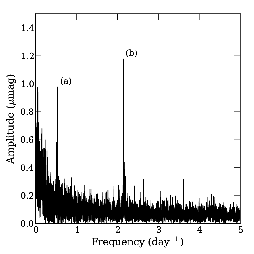
Figure 2: Frequency spectrum of residual data after removing the ellipsoidal variation as well as 182 of the largest-amplitude pulsations (see § 3.1). No pulsations have amplitude $\gtrsim 1.2\mu$mag. In the figure we have marked two of the largest-amplitude pulsations that we did not include in our global fits, as they have frequencies that are too close to other frequencies to be independently resolved in the data. The frequency marked (a) is close to F5, the largest-amplitude anharmonic pulsation. The peak marked (b) is close to F1, the largest-amplitude harmonic pulsation $f=90\Omega_{\rm orb}$.

Compared to W11, who detrended the data by completely masking the brightening events and then similarly fitting cubic polynomials, our method gives smaller residuals near the brightening events and smaller formal errors in the derived properties of the pulsations.

3 Sinusoidal pulsations in KOI-54

3.1 Observed frequencies, amplitudes, and phases

We systematically search for the $200$ largest-amplitude pulsations in the lightcurve by removing our best-fit ellipsoidal variation model and then iteratively removing the largest-amplitude pulsation found in the power spectrum of the residual data. Between steps, we simultaneously refit the data for the frequency, phase, and amplitude of all known pulsations. In practice, the process of refitting the data via least-squares can cause the frequencies of two or more initially distinct pulsations to converge. As a result, we remove 18 cases where the frequency spacing between two pulsations is less than the reciprocal of the total duration of observations (i.e., pairs that have not undergone one full beat in the window of observations), and simultaneously refit all the remaining $182$ pulsations.

In Table It takes a village to raise a tide: nonlinear multiple-mode coupling and mode identification in KOI-54, we present the $70$ largest-amplitude harmonic pulsations with frequency $f>20\Omega_{\rm orb}$ and $|f-k\Omega_{\rm orb}|<0.02\Omega_{\rm orb}$, where $k$ is an integer, along with their measured phase (from 0 to 1) with respect to the epoch of periastron as well as BJD$-2454833$. In Table It takes a village to raise a tide: nonlinear multiple-mode coupling and mode identification in KOI-54, we similarly present the $59$ largest-amplitude anharmonic pulsations with $|f-k\Omega_{\rm orb}|\geq 0.02\Omega_{\rm orb}$. The derived properties of low-frequency pulsations ($f<20\Omega_{\rm orb}$) have much greater uncertainties because of systematic trends in the raw data that we were unable to remove completely, so we do not report these pulsations in our results. After removing the $182$ largest-amplitude pulsations, we are left with no pulsations with amplitude $\gtrsim 1.2\,\mu$mag. To be consistent with W11 and much of the observing literature, we fit for the amplitude $A_{i}>0$, frequency $f_{i}$ and phase offset $\delta_{i}$, using the form $A_{i}\sin{2\pi(f_{i}t+\delta_{i})}$, where the time $t$ is measured relative to the epoch of periastron, $t_{p}$, as well as BJD-$2454833$. The variance in the residual lightcurve is $\approx 16\,\mu$mag, approximately 1.6 times larger than the photometric uncertainty of each observation. The frequency spectrum of the residuals is presented in Figure 2.

We estimate the formal uncertainties of our fits by a Monte Carlo method (for systematic uncertainties, see § 3.2). We create mock light curves using the best-fit parameters of the pulsations, using the same observing window as the real data. We then add Gaussian white noise to each point with an amplitude $10^{-5}$, consistent with the photometric uncertainty in each data point. Finally, we add $1/f$ noise to the data by passing it through the same high-pass Hann filter as the data, and then rescaling the amplitude of the $1/f$ noise so the final noise amplitude of the mock light curve equals the observed amplitude of the residuals. The power spectrum of the noise we generate matches both the amplitude and shape of the residual power spectrum much better than white noise alone, which is commonly used in other analyses. We refit each mock data set 100 times using the previously known best-fit parameters as our initial values, and report the variance of the best-fit parameters as the formal uncertainties in Tables It takes a village to raise a tide: nonlinear multiple-mode coupling and mode identification in KOI-54 & It takes a village to raise a tide: nonlinear multiple-mode coupling and mode identification in KOI-54.

For some pulsations that have similar frequencies, we find that fitting routine can be pathological, resulting in the two pulsations to be fit with the same frequency. Even when this happens in only one of the noise realizations, the reported formal uncertainty can be significantly larger than the intrinsic amplitude of the observed pulsation. In Tables It takes a village to raise a tide: nonlinear multiple-mode coupling and mode identification in KOI-54 & It takes a village to raise a tide: nonlinear multiple-mode coupling and mode identification in KOI-54 we report all observed pulsations with amplitudes larger than $\approx 0.7\mu$mag, which typically are $\approx 3\sigma$ local detections, and have not been corrected for searching over the entire parameter space. Some of these pulsations, especially the low-frequency anharmonic pulsations, may be noise. We choose to report all of these pulsations because any spurious pulsations do not contaminate our analysis.

3.2 Systematic uncertainties

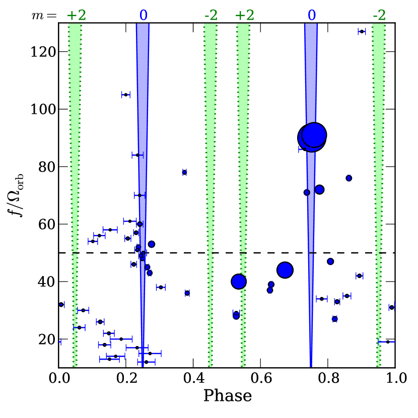
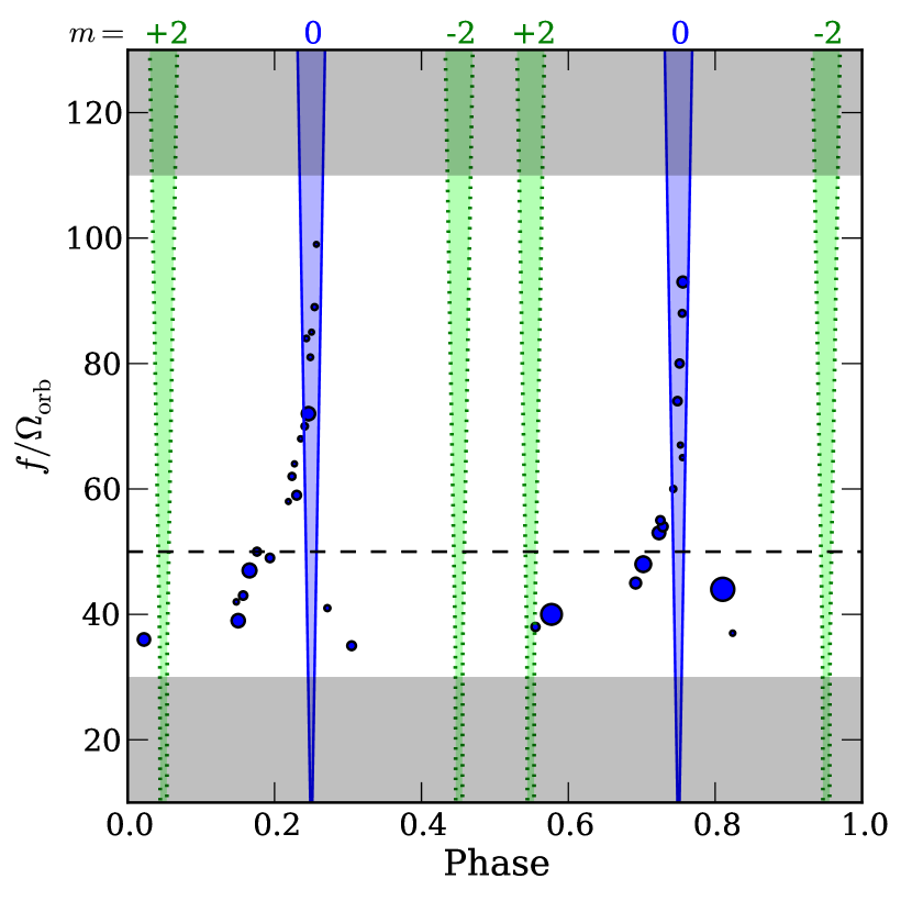
Figure 3: Phases of harmonic pulsations. Left: Plotted are phases of the near-perfect harmonics ($|f-k\Omega_{\rm orb}|<0.02\Omega_{\rm orb}$) of the orbital frequency relative to the best-fit epoch of periastron found by W11. The area of each circle corresponds to the amplitude of the pulsation. The vertical shaded cones correspond to the expected phase for $m=0$ (blue with solid lines) and $m=\pm 2$ (green with dotted lines) modes. The width of the cones result from the systematic uncertainties in the epoch of periastron as well as the argument of periastron. We conservatively assume that the systematic uncertainty in the epoch of periastron is $6\times$ larger than the quoted uncertainty in W11, consistent with our modeling. The actual system parameters, of course, correspond to only one line within each cone. For oscillations that are in a resonance lock, the phase of the pulsation can be nearly arbitrary. We see the 90th and 91st harmonics are consistent with being $m=0$ oscillations. For harmonics with $f/\Omega_{\rm orb}\lesssim 50$, the oscillations are expected to be traveling waves, and may have an arbitrary phase. We omit harmonics that have phase uncertainties greater than $0.015$. Right: The phase information of linearly driven oscillations in a theoretical binary system from B12, which is qualitatively similar to KOI-54. Only the response of $l=2$, $m=0$ oscillations are included in the calculation. We do not show results in the shaded regions where the linear response was not calculated. There is no uncertainty in the epoch of periastron in the theoretical model; the expected phases for low-amplitude $l=2$, $m=0$ pulsations should be offset from the center of the shaded cones.

Our work here, and work on similar systems, inevitably possesses important systematic errors. The greatest uncertainty in our calculations is the systematic uncertainty in fitting for the epoch of periastron, which impacts the derived phase offsets of the harmonic pulsations. Indeed, in W11, the authors’ best-fit epoch of periastron derived from radial velocity data alone is $6\sigma$ away from the epoch found using radial velocities together with photometry. Visually, the systematic errors in the fitting of the RV data appear more significant. The quoted uncertainties in the W11 RV data were also probably too low due to heterogeneity of the spectra (G. Marcy, private communication). For this reason, we exclusively use the photometrically determined epoch of periastron. In addition, fitting only $15$ of the largest-amplitude pulsations, as done in W11, is likely insufficient for determining the epoch of periastron. As we will show in § 4 (see Fig. 3), many of the low-amplitude pulsations are $m=0$ oscillations that reach their maximum near periastron and bias the fitting of the ellipsoidal variation and irradiation of the binary. Indeed we found that the peak amplitudes of the observed brightening events were $80\,\mu$mag larger than the best-fit model if the pulsations are not taken into consideration.

In W11, the authors compensated for the undetected pulsations by increasing the uncertainty of each data point by a factor of $10$, thereby obtaining a normalized $\chi^{2}$ less than unity. Nevertheless, systematic errors from the undetected pulsations may remain. We attempt to ascertain how the pulsations bias the epoch of periastron by refitting the detrended data simultaneously with 15 or 30 of the largest-amplitude pulsations. We find systematic changes in the epoch of periastron approximately three times larger than the uncertainty reported in W11. We conservatively estimate that the true uncertainty is six times larger than reported in W11 (Table 2).

Unfortunately, many of the low-frequency pulsations are systematic errors from our fitting routine using cubic polynomials. We therefore fit the pulsations by both including all low-frequency pulsations and compare this to the fit excluding pulsations with $f<20\Omega_{\rm orb}\approx 0.5\,$day^-1. We find that the difference in the fits of the high-frequency pulsations are less than the formal uncertainties listed in Tables It takes a village to raise a tide: nonlinear multiple-mode coupling and mode identification in KOI-54 & It takes a village to raise a tide: nonlinear multiple-mode coupling and mode identification in KOI-54. We also note that we do not include the impact of Doppler boosting in our light curve models. We find that including the impact of boosting does not change the amplitude of any pulsations by more than $0.5\,\mu$mag, although the Doppler boosting signal is important in other eccentric binaries reported by Kepler that show strong tidal distortions (Thompson et al., 2012; Hambleton et al., 2013).

Incompletely subtracting the ellipsoidal variation can also systematically contaminate our fits of the harmonic pulsations. Fortunately, the Fourier decomposition of the ellipsoidal variation is continuous with frequency. We estimate that the total contamination is $\lesssim 0.3\mu$mag by inspecting the limits we placed on the amplitude of undetected harmonic pulsations. A similar technique may be useful when constraining the contamination of lower harmonics in less eccentric binaries.

4 Linearly driven harmonic pulsations

Each star is expected to have tidally driven pulsations at perfect harmonics of the orbital frequency $\Omega_{\rm orb}$. In § 4.1 we briefly outline the general theory of dynamical tides and describe how the pulsations reveal detailed properties of the star (B12, Fuller & Lai 2012). In § 4.2 we analyze the phases of the harmonic pulsations relative to periastron in order to determine the azimuthal order, $m$, of the oscillations. In § 4.3, we search for time variability in the amplitudes, phases, and frequencies of KOI-54’s pulsations.

4.1 Introduction

For a nonrotating star, the time-varying tidal potential excites $l\geq 2$ mode spherical harmonics in the star. The oscillations within the star are observed as sinusoidal pulsations, which are averaged over the disk of the entire star. The steady-state, equilibrium solution is simply a sinusoidal pulsation with an observed frequency $k\Omega_{\rm orb}$ that is a harmonic of the orbital frequency, where $k$ is an integer. The amplitude and phase of the pulsation are determined by how well tuned the oscillator is relative to an eigenfrequency as measured by the detuning $\delta\omega=\omega_{nl}-k\Omega_{\rm orb}$, by the damping rate of the excited mode $\gamma_{nl}$, as well as by the spatial coupling between the driving force and the mode (Press & Teukolsky, 1977). By directly measuring the amplitude and phase of a harmonic pulsation, it is possible to determine the detuning-to-damping ratio $\delta\omega/\gamma_{nl}$, as well as the azimuthal order of the oscillation, $m$.

The phases of observed pulsations of a star are determined by disk averages of the flux perturbations on the stellar surface. In this work we measure the phase of the pulsation from the light curve using the equation (see § 3.1)

$$A_{i}\sin{2\pi(f_{i}t+\delta_{i})},$$ (1)

where $A_{i}>0$, and $t$ is measured relative to the epoch of periastron, $t_{p}$. The observed phase of the pulsation directly depends on the order of the harmonic, $m$. B12 derived the observed pulsation phase relative to the epoch of periastron to be

$$\delta=\left(\frac{1}{4}+\Psi_{nlmk}+m\phi_{0}\right)\mod\frac{1}{2},$$ (2)

where $\phi_{0}=1/4-\omega_{p}/(2\pi)\mod 1$, $\omega_{p}$ is the argument of periastron of the orbit,

$$\Psi_{nlmk}=-\frac{1}{2\pi}\arctan{\left(\frac{\omega_{nl}^{2}-\sigma_{km}^{2}}{2\gamma_{nl}\sigma_{km}}\right)}\mod\frac{1}{2},$$ (3)

and $\sigma_{km}=k\Omega_{\rm orb}-m\Omega_{*}$ is the driving frequency of the tide in the corotating frame of the star with rotation frequency $\Omega_{*}$. We expect that most excited oscillations are poorly tuned, i.e., $|\delta\omega|\gg\gamma_{nl}$, since the frequency spacing of the eigenmodes is much larger than the damping rate of high-frequency g-modes. In this limit, equations 2 & 3 reduce to

$$\delta=\left(\frac{1}{4}+m\phi_{0}\right)\mod\frac{1}{2}.$$ (4)

Since $\phi_{0}$ is a quantity derived from modeling the equilibrium tide as well as the radial velocity data, we can directly determine the order of an oscillation $m$ in this limit.

In this work, we report the absolute phases of the pulsations $\in[0,1)$ relative to the epoch of periastron using the sine function to be consistent with the observing literature (see § 3.1). A pulsation is observed at its maximum at the epoch of periastron when $\delta=1/4$. For $m=0$ modes, based on equation 4 we would expect the pulsation to be near maximum ($\delta\approx 1/4$) or near minimum ($\delta\approx 3/4$) at the epoch of periastron. B12 show that if the largest-amplitude harmonics of KOI-54 are $m=0$ modes, then their detuning-to-damping ratio is $|\delta\omega|/\gamma_{nl}\sim 20$ and so should be offset from $1/4$ or $3/4$ by no more than a few percent. Given the face-on orientation of KOI-54, most observable pulsations should be $m=0$, $l=2$ modes. Large amplitude $m=2$, $l=2$ pulsations may also be present, but the amplitudes of these pulsations are suppressed by a factor of $\sin^{|m|}{i}\approx 1/200$.

There are two other regimes where equation 4 does not apply. First, when oscillations are no longer standing waves but are instead in the traveling regime, the phases begin to deviate from equation 4, which we discuss in more detail in § 4.2.2. Second, when an excited mode is in a resonance lock, it is possible that $\delta\omega/\gamma_{nl}\sim 1$, allowing for a potentially arbitrary phase. Such a resonance lock can only occur when $m\neq 0$. For stars similar to KOI-54, each star is expected to be in a resonance lock only $\sim 10\,$percent of the time, and as discussed in B12, it is much rarer for both stars to be in a simultaneous lock.

As we have discussed, for most of the large-amplitude pulsations, only one eigenmode of a single star will contribute to the corresponding pulsations. However, Kepler photometry is so precise that we are able to detect pulsations with amplitudes comparable to $1\,\mu$mag. A fraction of these low-amplitude pulsations will have contributions from both stars or from multiple modes in a single star.

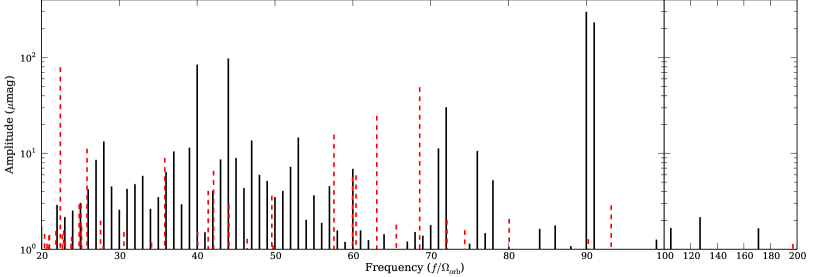
Figure 4: Distribution of pulsation amplitudes down to $1\,\mu$mag. The pulsations with frequencies consistent with perfect harmonics of the orbital frequency ($|f-k\Omega_{\rm orb}|<0.02$) are shown with black lines. The anharmonic pulsations are shown with red dashed lines. Note: the frequency scale changes at $f/\Omega_{\rm orb}=100$.

4.2 Harmonic pulsation phases

4.2.1 Standing waves

In Figure 3, we plot the phases of the harmonic pulsations as well as the phases in a theoretical model from B12. The model was derived to qualitatively match the amplitudes and frequencies of observed pulsations in KOI-54. In both plots, the area of each point is in proportion to the observed amplitude of the pulsation, the error bars show the uncertainties in the phase, and the filled vertical regions of the plot show the phases expected for $m=0$ and $m=\pm 2$ modes (§ 4.1, equation 4). For standing waves, with $k\equiv f/\Omega_{\rm orb}\gtrsim 50$ (see § 4.2.2 for traveling waves), we expect the $m=0$ oscillations to have phases near $1/4$ and $3/4$ (§ 4.1). Many of the observed pulsations are consistent with this result (e.g., F1, F2, F7, F11, and F16 among others). In particular we find that the phases of the largest-amplitude 90th and 91st harmonics, $.752\pm.0001\,$(statistical)$\,\pm 0.013\,$(systematic) and $.759\pm.0001\,$(statistical)$\,\pm 0.013\,$(systematic) are consistent with being $m=0$ modes. If either of these pulsations were in a resonance lock, its phase could be arbitrary (when $\delta\omega/\gamma_{nl}\sim 1$; § 4.1).

There are a number of pulsations that appear to be $m\neq 0$ modes, e.g., F18, F32, F67, & F68. Not shown in the figure is the pulsation with $k=171$ (F68) which has a phase near $0.5$. This is consistent with what we expect for a typical $m=2$ oscillation, especially given its low observed amplitude, which excludes it as originating from a resonance lock. The phase of the 105th harmonic (F67) is closer to the phase expected for an $|m|=3$ oscillation. The phase of the 76th (F18) and 127th (F57) harmonics are consistent with $m=1$ modes.

There are at least four possible explanations for why some pulsations do not have phases that correspond to $m=0$ modes in Figure 3. 1) The oscillation is an $m\neq 0$, $l\geq 2$ mode. 2) Given the large number of excited pulsations, we might expect a few of the pulsations from each star to interfere. This causes the observed phase to shift between the intrinsic phase of each star when $\delta_{A}\neq\delta_{B}$. The observed phase of the pulsation, $\delta_{AB}$, is

$$\delta_{AB}=\frac{1}{2\pi}\cos^{-1}{\left(\frac{A_{A}\cos{2\pi\delta_{A}}+A_{B}\cos{2\pi\delta_{B}}}{A_{AB}}\right)}$$ (5)

where the amplitude of the resulting pulsation is

$$A_{AB}=\sqrt{A_{A}^{2}+A_{B}^{2}+2A_{A}A_{B}\cos{2\pi(\delta_{A}-\delta_{B}})}.$$ (6)

3) If the oscillation is primarily driven by nonlinear terms via three or higher mode coupling its phase will no longer reflect the expected linear offset (see § 5). 4) Lastly, if it is an $m\neq 0$ oscillation that was shifted from the traveling wave regime because of the star’s rotation, then it could also have an arbitrary phase. For our outliers, this is possible only if $\Omega_{*}\gtrsim 13\Omega_{\rm orb}$, which is satisfied by the expected rotation rate of the star (B12).

It is unlikely that 90th and 91st harmonic pulsations originate in the same star. For $k\sim 90$, the typical frequency spacing between the eigenfrequencies of $m=0$, $l=2$ g-modes is significantly larger than $\Delta k\sim 1$. Indeed, the g-mode eigenfrequencies of a star are expected to behave asymptotically as (Christensen-Dalsgaard, 2003)

$$\omega_{ln}\approx\omega_{0}\frac{l+1/2}{(n+\alpha)\pi},$$ (7)

where we assume that $l=2$ and $n\gg 1$. Assuming that $m=0$ for both the $k=90$ and $k=91$ pulsations, we can estimate where other large amplitude $m=0$ fluctuations should exist using stellar models or by tuning equation 7. Just as importantly, when a pulsation appears with the frequency between two consecutive eigenmodes, we can conclude $|m|>0$, since it must have been shifted from stellar rotation by $m\Omega_{*}$. We can calibrate equation 7 by finding the eigenfrequencies of stellar models with parameters near the best-fit found by W11. We use an untuned MESA stellar model (Paxton et al., 2011) for a star similar to those in KOI-54 to calibrate equation 7 at $n\approx 10$–$20$. We find the best-fit parameters are $\alpha\approx 1.07$ and $\omega_{0}=40.5\,$d^-1.

Assuming that $n=14$ for $k=90$, we roughly estimate that the next few eigenfrequencies are near $83.5$, $79$, $74.5$, $70.6$, $63.8$, $60.8$, $58.1\Omega_{\rm orb}$, where the uncertainty is of order $\Delta k\approx 1$. Interestingly there are two large-amplitude pulsations in KOI-54 with $k=71$ and $k=72$, both with phases consistent with $m=0$, which may correspond to the $n=18$ modes of each star. There are no pulsations with amplitudes $\gtrsim 1.7\,\mu$mag between where we expect the $n=14$ and $n=15$ pulsations. Identifying the eigenfrequencies of the stars in this manner can greatly reduce the large computational overhead of finding stellar models that reproduce the properties of the two stars. The frequency spacing between the high-frequency pulsations, with $f\gtrsim 100\Omega_{\rm orb}$, is also consistent with the MESA models of B12.

Figure 3 shows how the phases of the pulsations are a powerful tool to determine the nature of the pulsations (e.g., the azimuthal order, $m$, or whether a mode is in a resonance) as well as to verify the epoch of periastron and $\phi_{0}$.

4.2.2 Traveling waves

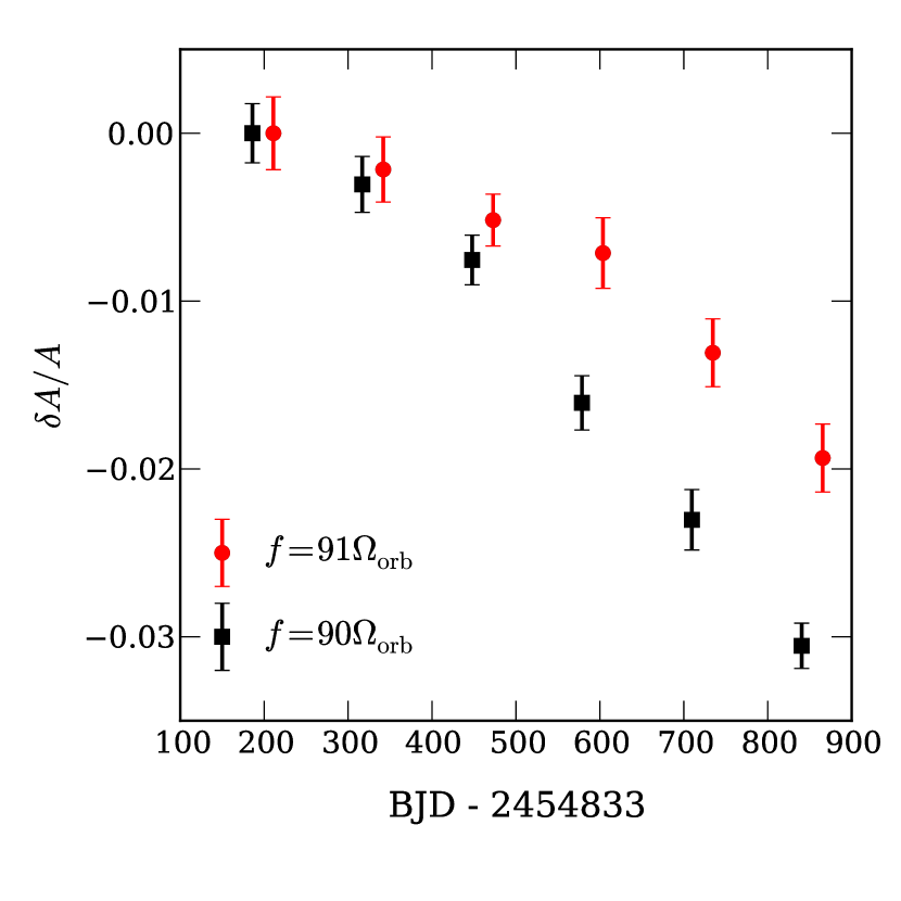
Figure 5: Fractional amplitude change ($\delta A/A$) of the $k=90$ and $k=91$ pulsations over time. The error bars show the estimated standard deviation of the fits for each individual time bin. The $k=91$ data points are offset from the center of the bin in order to increase legibility.

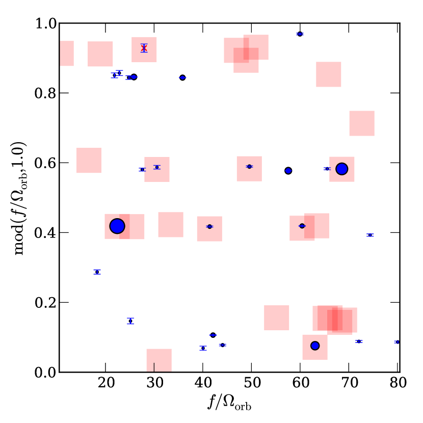
Figure 6: Distribution of anharmonic pulsation frequencies. Plotted is the fractional part of $f/\Omega_{\rm orb}$ as a function of $f/\Omega_{\rm orb}$ for the anharmonic pulsations of KOI-54. The area of each circle corresponds to the amplitude of the pulsation. Assuming that the nonlinear coupling is with the 91st harmonic, the complementary daughter modes to the anharmonic pulsations are shown as pink squares, where $f_{\rm complement}\equiv 91\Omega_{\rm orb}-f$. Four pairs of the observed anharmonic pulsations add to $91\Omega_{\rm orb}$ within their uncertainties: F5 & F6, F8 & F100, F25 & 76, and F39 & F42. The other pulsations either have complementary pairs that are not visible, or are the daughter modes of other pulsations. This figure only shows the pulsations that have frequencies $f/\Omega_{\rm orb}>20$ and amplitudes $>1.0\,\mu$mag.

At lower frequencies, the group travel timescale of the wave becomes comparable to the damping timescale near the surface at the outer turning point of the mode. This results in a phase offset of the wave of order $\sim\sqrt{t_{\rm group}/t_{\rm damp}}$. As such, pulsation phases need not obey the relation in equation 2. B12 estimated that this should occur for $k\lesssim 50$ for stars similar to KOI-54 when $m=0$. These estimates were made under the approximation of solid-body rotation. For differentially rotating bodies, the shear between layers could dramatically impact the onset of the traveling wave regime, resulting in much larger phase offsets for frequencies $\omega\lesssim 2\Omega_{*}$ (Goldreich & Nicholson, 1989). Only rapidly rotating stars, with much faster spins than expected for KOI-54 (B12), would impact the phases for frequencies much larger than $50\Omega_{\rm orb}$.

The horizontal dashed line in Figure 3 marks where $k=50$, approximately when the onset of the traveling regime is expected (B12). We see that below this frequency there are more observed pulsations with phases that are not consistent with $m=0$ standing waves. The phases of the two large-amplitude harmonics, $k=44$ (F3) and $k=40$ (F4), in particular, are significantly offset from the phases of the $k=90$ and $k=91$ pulsations. The phase offsets of traveling waves in KOI-54 appear comparable to the phase offsets in the best-fit semi-quantitative model of B12 (right panel of Fig. 3). For modes with $m\neq 0$, the traveling wave regime is determined by the frequency of the tide in the corotating frame, which is Doppler shifted from the observers frame by $k\Omega_{\rm orb}-m\Omega_{*}$. For $m>0$, modes with $k\gtrsim 50$ can still be in the traveling wave regime, especially when it is rotating rapidly. In principle, the rotation frequency of the star may be inferred by identifying where the $m>0$ modes enter the traveling wave regime.

We note again that as the pulsation amplitude decreases, it is more likely that modes from both stars will have comparable contributions to the pulsations. This can occur at any frequency, but is more likely at lower frequencies where the spacing between eigenfrequencies is smaller (eq. 7). When this happens, the observed phase will be determined by a combination of the pulsation amplitudes and phases.

4.3 Time variation of the pulsations

The estimated timescale for KOI-54 to circularize is very long, $\sim 10^{10}\,$yr, compared to the duration of the observations, so we do not expect variations in the orbital elements to be directly observable with the current data set. However, the amplitude and phases of the pulsations in KOI-54 can vary on much shorter timescales, especially if the pulsations are in a nonlinear limit cycle (Wu & Goldreich, 2001) or are close to resonance ($\delta\omega\sim\gamma$). We therefore search for time variation in the amplitudes, frequencies, and phases of the pulsations. To do so we split the data into 6 bins each with equal duration of $131\,$d, and refit each with the $60$ largest-amplitude pulsations. We omit 7 pulsations from these fits because their frequencies are spaced too closely together to resolve in the shorter duration of the observations. We measure the uncertainty in each fit in the same way as for the overall uncertainties: via a Monte Carlo method with a $1/f$ plus white noise spectrum (see § 3.1).

Figure 5 shows how the amplitudes of the 90th and 91st harmonic pulsations vary with time. We find that their amplitudes declined by $3$ and $2$ percent, respectively, over the duration of the observations. The characteristic timescales associated with the changes are $A/{\dot{A}}\approx 60$ and $90$ years for the 90th and 91st harmonics, respectively. If the entire change in amplitude was systematic, we would expect the change to be the same in both pulsations, but they are different at the 3$\sigma$ level. We find similar variations in the amplitude of the two pulsations when using only four or five bins, or when looking at individual quarters of the Kepler data.

To check that our estimated errors are correct, we compare the distribution of $\delta A/A$ to the estimated error for all of the observed pulsations. Excluding the outliers beyond four standard deviations, we find the estimated errors are only 25 percent smaller than the variance in $\delta A/A$. Finally, if the changes are indeed systematic, we would expect the brightening events at pericenter to show a similar evolution. A $3\,$percent error in the absolute calibration of the source would reduce the peak amplitude of the tidally induced static tide and irradiation by $\approx 240\,\mu$mag over the observed duration of the brightening events. We do not see signatures of this deviation in the residuals near the brightening events even if we only subtract the 20 brightest pulsations.

Such a large change in the amplitude of the pulsations is not expected. The timescale for the changes is comparable to the damping time for $n=14$ g-modes. Even if the oscillations are close to resonance, which we have already argued the $k=90$ and $k=91$ modes are likely not, the maximum change in amplitude expected is of order

$$\frac{\delta A}{A}\sim\frac{\Delta t}{t_{\rm tidal}}\frac{\omega_{nl}}{\gamma_{nl}},$$ (8)

where $\Delta t$ is the duration of the observations, $t_{\rm tidal}$ is the characteristic timescale for tides to change the orbital parameters, $\gamma_{nl}\approx 1(n)^{4}\,$Myr^-1, with $n=14$ for $k\approx 90$ in KOI-54 (W11, B12). Alternatively we can invert equation 8 to get $t_{\rm tidal}$, the timescale of the change in the orbital parameters. For $n=14$ and $\gamma\approx 4\times 10^{-2}\,$yr^-1, $\Delta t\approx 3\,$yr, we derive $t_{\rm tidal}\lesssim 10^{6}\,$yr. This is a strong upper limit, and is shorter than the expected synchronization timescale by a factor of $\sim 80$ (B12).

As we alluded to earlier, one possible explanation of our observations is that the modes in question are undergoing limit cycles as a result of parametric decay (§ 5). This is expected to occur when the frequency offsets of the daughter modes are less than their damping rates (Wu & Goldreich, 2001). The timescale associated with the limit cycle, which is $\sim\gamma^{-1}$, is comparable to the inferred timescale for the amplitude changes.

However, in § 5.2, we find no evidence to suggest that the $k=90$ pulsation is undergoing parametric decay. However, nonlinear second-order coupling between groups of oscillators can result in chaotic behavior in many circumstances. This can occur even when the oscillators have the same resonant frequency (e.g., Kuramoto & Battogtokh, 2002).

More data or a more sophisticated detrending routine that explicitly preserves long term trends may be able to determine whether some the variation of the pulsation amplitudes is systematic or if the variations are intrinsic to KOI-54. Systematic variations of approximately one percent have been observed in the transit depths of the Hot Jupiter HAT-P-7b (Van Eylen et al., 2013). The systematic effects were found to be seasonal, relating to the rotation of the Kepler spacecraft. However, Van Eylen et al. (2013) found no evidence of systematic trends when comparing data between the same season. We find that the amplitudes of the 90th and 91st harmonic pulsations decreased with time, even when compared to the same season of data. Finally, we note that nodal regression owing to a third body could change the amplitudes of $m\neq 0$ pulsations by altering the inclination of the system. This would additionally cause changes to the amplitude of the equilibrium tide, which we do not observe.

5 Nonlinearly excited tides

5.1 Introduction

If a mode achieves a large enough amplitude, the linearized fluid equations are no longer sufficient to describe its evolution. Instead, it may decay into daughter modes via the parametric instability. Traditionally, this has been calculated as a form of resonant three-mode coupling that minimizes the threshold for the instability to develop (e.g., Dziembowski 1982, Wu & Goldreich 2001, B12, Fuller & Lai 2012). These daughter modes increase the rate at which energy is damped in the star, potentially accelerating the impact of the tides. KOI-54 exhibits a variety of pulsations that have frequencies which are not integer harmonics of the orbital period. In §5.2, we will explore the distribution of anharmonic pulsations in KOI-54 in the context of isolated three-mode coupling. We will show in § 5.3 that these anharmonic pulsations are best explained as the nonlinearly excited daughter modes of several different parent modes.

Modes can efficiently couple to each other in the second order when they are near resonance, i.e., when

$$|\omega_{A}-(\omega_{a}+\omega_{b})|=|\delta\omega_{Aab}|\ll|\omega_{A}|,$$ (9)

where we denote the primary parent mode with the capital subscript $A$ and the the pair of daughter modes as lowercase $a$ and $b$. They must also satisfy certain selection rules:

$$m_{A}=m_{a}+m_{b},$$ (10)

$$\mod(l_{A}+l_{a}+l_{b},2)=0,$$ (11)

and

$$|l_{a}-l_{b}|\leq l_{A}<l_{a}+l_{b}.$$ (12)

Not only do the intrinsic frequencies of the excited oscillations sum to the parent frequency, but equation 10 also implies that the frequencies of the observed daughter pulsations also sum to the parent frequency:

$$f_{a}+f_{b}=f_{A}$$ (13)

For sufficiently small-amplitude oscillations, the daughter modes do not grow, and the instability is suppressed. The daughter modes will only grow in amplitude when the parent mode is sufficiently excited for the parametric instability to develop (see, e.g., B12).

All modes with $l_{a}=l_{b}$ have nonzero coupling coefficients. However, for KOI-54 the coupling becomes much less efficient when $l_{a,b}\gg 2$ (B12), so we restrict our attention to $l_{a,b}\leq 3$. For parent modes with $m_{A}=0$, equation 10 implies $m_{a}=-m_{b}$. Although the onset of parametric decay occurs at relatively large amplitudes, the complete triplet of modes should not necessarily be visible in the Kepler observations. In many cases the parent mode or one of the daughter modes can have an amplitude that is much smaller than any of the other oscillations (see, e.g, B12). Additionally, because KOI-54 is nearly face on, the visibility of $m\neq 0$ oscillations is suppressed by $\sin^{|m|}{i}\approx(1/10)^{|m|}$.

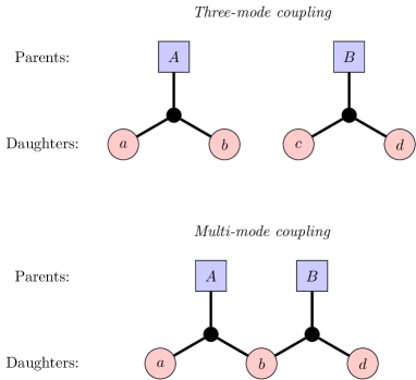
Figure 7: Diagram of traditional, isolated three-mode coupling versus multiple-mode coupling. The top panel shows two sets of three coupled modes. In previous nonlinear analyses, these sets are treated independently of the other. The bottom panel shows a coupled system of five modes. It is the same as the top panel—both are coupled at second-order—except the two parent modes share the coupled daughter mode $b$. KOI-54 shows evidence for at least three parent modes coupled to each daughter mode. Because the coupling still occurs at second-order, the selection rules for strong coupling still apply to multiple-mode coupling. Namely, for the bottom panel, $f_{a}+f_{b}=f_{A}$, $m_{a}+m_{b}=m_{A}$, and additionally $f_{b}+f_{d}=f_{B}$ and $m_{b}+m_{d}=m_{B}$.

5.2 Three-mode coupling and the observed distribution of daughter pairs

The anharmonic pulsations in KOI-54 are best explained as daughter modes that are nonlinearly excited by higher-frequency tidally driven oscillations. As expected from equation 13, many of the anharmonic pulsations have frequencies that, when summed, equal the frequencies of some of the largest-amplitude harmonic pulsations within the formal precision of the measurements. The two most prominent are the F5 ($f_{5}=22.419\Omega_{\rm orb}$) and F6 ($f_{6}=68.582\Omega_{\rm orb}$) pulsations, which appear to be daughter modes of the 91st harmonic of the orbital period. These were the only two anharmonic pulsations reported in W11 that were consistent with being a complete daughter mode pair of the $91$st harmonic (B12, Fuller & Lai 2012). Here we report a total of four pairs of anharmonic pulsations which have frequencies that all add to $91\Omega_{\rm orb}$. We additionally find that the frequencies of many anharmonic pulsations sum to other harmonic parents, specifically $f_{7}=72\Omega_{\rm orb}$ and $f_{11}=53\Omega_{\rm orb}$. These three parent modes in particular have frequencies that are equally spaced with $\Delta f/\Omega_{\rm orb}=\Delta k=19$. We address this in more detail in § 5.3.

In Figure 6, we plot the frequency ($f/\Omega_{\rm orb}$) and fractional part of the frequency ($f/\Omega_{\rm orb}\mod{1.0}$) for each anharmonic pulsation with measured amplitude $>1.2\,\mu$mag. The area of each circle is proportional to the amplitude of the pulsation. For each point in the graph, we also highlight the complementary “sister” frequency of the pulsation with a pink square, assuming that it is a daughter of the $k=91$ harmonic. In other words, the pink squares represent frequencies that satisfy $f_{\rm complement}\equiv 91\Omega_{\rm orb}-f$. There are eight points that are highlighted in pink, corresponding to four complete daughter pairs of the 91st harmonic. The vast majority of the observed anharmonic pulsations, however, do not have complementary pairs with amplitudes above $1.2\,\mu$mag. As discussed in § 5.1, this is consistent with theoretical expectations. No two observed anharmonic pulsations add to $k=90$.

There are two striking features of the distribution of frequencies plotted in Figure 6. First, many of the pulsations have regular frequency spacing. For all the completely observed daughter pulsation pairs, there are other observed anharmonic pulsations with frequencies separated by $\Delta f=\Delta k\Omega_{\rm orb}=19\Omega_{\rm orb}$. For example, $f_{5}+f_{6}=f_{1}=91\Omega_{\rm orb}$, but another complementary mode sums to the fifth largest-amplitude harmonic pulsation, $f_{5}+f_{42}=(91-19)\Omega_{\rm orb}=f_{7}=72\Omega_{\rm orb}$, and to the sixth largest-amplitude harmonic pulsation $f_{5}+f_{76}=f_{11}=(91-2\times 19)\Omega_{\rm orb}=53\Omega_{\rm orb}$. A similar pattern emerges for the daughter pair of F8 and F100: $f_{8}+f_{100}=f_{1}$, $f_{49}+f_{100}=f_{7}$ and $f_{47}+f_{100}=f_{11}$. Although it is possible that this is just a coincidence, we are compelled to suggest that all of these nonlinearly driven daughter pairs share multiple parent modes. In the case of KOI-54, three of most prominent parent modes are separated by $\Delta f=19\Omega_{\rm orb}$. This particular value of $19$ is probably set randomly by the eigenfrequency spacing unique to one of the stars. Additionally, each parent mode clearly has multiple daughter pairs. As we will discuss in § 5.3, the coupling between multiple parents and daughters is one possible explanation for why the amplitude of the 91st harmonic is so much lower than the threshold estimated using only isolated three-mode coupling (B12).

The second salient feature of the anharmonic pulsations is that many share common fractional (noninteger) parts in units of the orbital frequency, as was first noted by W11. There are eight pulsations that have frequencies with fractional parts near $0.42$ (F5, F25, F39, F80, F87, F110, F124, & F128) , and nine observed pulsations that have frequencies with their fraction part $0.58$ (F6, F9, F42, F61, F63, F76, F102, F123, & F130). That is, if you sum the frequencies of one pulsation from each group you will get a harmonic (integer) frequency. There are also six pulsations with the fractional part of their frequency near $0.08$ (F8, F47, F49, F58, F59, & F75). There are eight near $0.84$ (F17, F19, F48, F71, F72, F86, F108, & F125). What would cause all the pulsations to share similar fractional parts? Again, we are led to the situation where each daughter is being nonlinearly excited by multiple parents. We explore this further in § 5.3.

The anharmonic pulsations can also be susceptible to the parametric instability. In this scenario, the daughter modes will themselves couple to granddaughter modes, which must obey the same restrictions (eqs. 10-12). We do not find evidence for granddaughter modes in KOI-54. However, it would be more difficult to observe daughters of the already low-frequency anharmonic pulsations in KOI-54. The frequency of the largest-amplitude anharmonic pulsation is close to the frequency cutoff we have imposed in our search for pulsations ($\approx 20\Omega_{\rm orb}$). Only a pulsation with amplitude $\gtrsim 10\,\mu$mag would be observable above all the noise at low frequencies.

5.3 Multiple-mode coupling in KOI-54

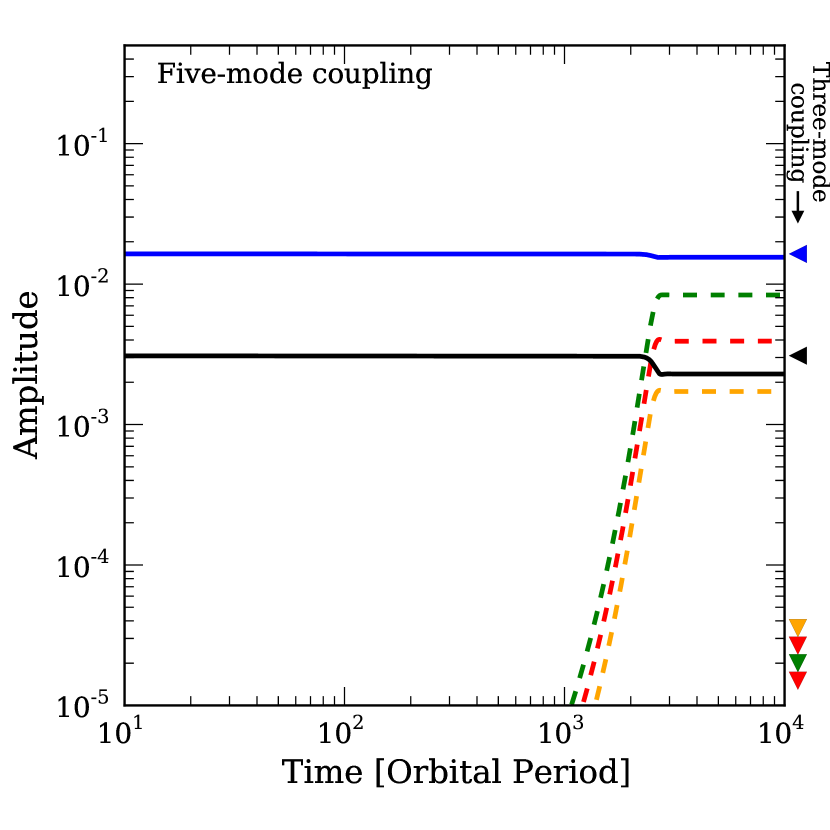
Figure 8: The onset of the parametric instability for a network of five oscillators coupled at second-order. In both panels the solid lines show the two parent modes, while the dashed lines show the three daughter modes for a system of five coupled oscillators. The triangles on the right show the final amplitude of the oscillations when we integrated the equations for two independent sets of three-mode coupling (as shown the top diagram of Fig. 7). The downward facing triangles indicate that the daughter modes did not grow in amplitude. In the left panel, the system undergoes the parametric instability only when treated as five coupled oscillators. The threshold for the onset of the parametric instability is decreased by approximately a factor of two compared to isolated three-mode coupling. The right panel shows how multiple mode coupling can redistribute the energy among the different excited modes. In this case, the largest amplitude parent mode is not the one that underwent parametric decay, but rather was powered by nonlinear interactions. We note that we did not account for the parametric instability of the daughter modes, and so these solutions are not complete, rather they are representative of the complex coupling in a network of oscillators in a tidally excited star.

As described in § 5.2, we find that the anharmonic pulsations have two features that are not explained in the traditional picture of three-mode coupling between individual overstable parent modes and their daughter modes. First, many anharmonic pulsations have frequency offsets from a perfect harmonic (residual fractions) that are nearly identical, and second, many observed pairs have common frequency differences of $\Delta f=19\Omega_{\rm orb}$. We propose that the distribution of frequencies in the anharmonic pulsations is naturally explained by coupling between groups of daughter pairs and parents. Figure 7 contrasts the case of isolated three-mode coupling, as we described in § 5.1, and multiple-mode coupling, as we describe further here. Throughout this section, we use the same terminology as B12.

A common simplifying assumption employed in deriving the nonlinear parametric instability is to consider coupling only within isolated mode triplets. We show this in the top diagram of Figure 7. By minimizing over all possible sets of three modes, constrained by equations 10 – 12, one can estimate when the parametric instability should develop (e.g., Dziembowski 1982, Wu & Goldreich 2001). Recently, Weinberg et al. (2012) extended the traditional isolated three-mode coupling calculations as described in § 5.1 to include the case of a single parent with $N$ distinct daughter pairs. The authors found this can reduce the threshold for the parent to become unstable by $\approx 1/N$. More generally, however, each eigenmode of the star can additionally couple to multiple parent modes in second-order perturbation theory, as we show in the bottom diagram of Figure 7. We explore this scenario by analyzing the system of equations for five coupled oscillators: two linearly driven parent modes and two daughter pairs that share a common eigenmode. We ask 1) does multiple-mode coupling result in the same quantitative peculiarities that we observed in § 5.2? and 2) does multiple-mode coupling lower the threshold for the parametric instability to develop?

Under the assumption of an equilibrium solution, i.e., that each eigenmode is a sinusoid with a fixed frequency $f_{i}$ and amplitude $A_{i}$, the observed frequencies will naturally reproduce the trends in the system. For a network of five oscillators coupled at second-order, the frequencies of the daughter pairs obey the relations $f_{a}+f_{b}=f_{A}$ and $f_{b}+f_{d}=f_{B}$ in order for the presumptive sinusoidal time dependence to cancel out. If the daughters are coupled to linearly driven parents, then both $f_{A}$ and $f_{B}$ will be harmonics of the orbital frequency, $k_{A,B}\Omega_{\rm orb}$. It then holds that $f_{a}-f_{d}=f_{B}-f_{A}$ must also be an integer multiple of $\Omega_{\rm orb}$. Thus, nonlinear multiple-mode coupling in eccentric binaries manifests itself with harmonic frequency differences between the anharmonic pulsations, just as we observe in KOI-54. This property is specific to dynamically excited tides in eccentric binaries. Parent oscillations that are driven by instabilities will not have integer spacing. As such, it becomes less likely that a daughter mode will couple to many parents.

Although it is a simple matter to derive the relationship between the frequencies of a network of five oscillators that are coupled to second-order, it is not clear if there is a closed-form analytic equilibrium solution for a network of five (or more) coupled oscillators, as the steady-state solution of three-mode coupling is already nontrivial. Instead, we integrate the coupled equations numerically to look at the consequences of multi-mode coupling on the steady state properties of the pulsations. In this calculation, we use realistic damping and driving rates as well as coupling coefficients computed in B12. The two parents are linearly driven by the tidal potential at $91\Omega_{\rm orb}$ and $72\Omega_{\rm orb}$. In this calculation, we use realistic damping and driving rates as well as coupling coefficients computed in B12. The two parents are linearly driven by the tidal potential at $91\Omega_{\rm orb}$ and $72\Omega_{\rm orb}$. Rather than trying to represent KOI-54 exactly, we arbitrarily choose the frequencies of the parents and daughter pairs to be close to resonance to demonstrate the impact of multi-mode coupling. We show the results of two calculations in Figure 8. In the two simulations, the intrinsic parent mode frequencies are ($91.295\Omega_{\rm orb}$, $72.044\Omega_{\rm orb}$) and ($90.615\Omega_{\rm orb}$, $71.996\Omega_{\rm orb}$). In one case, shown in the left panel, the system undergoes the parametric instability only when the set of five coupled oscillators are solved. When we treat the oscillators as two independent triplets, the parents are stable, and no daughter modes are excited. In the right panel, we show a case where the amplitude of the parent that undergoes the parametric instability actually ends up pumping energy into an initially low-amplitude linearly driven oscillation (which was stable in the isolated three-mode calculations).

To summarize, some consequences of nonlinear multi-mode coupling are: 1) the frequencies of many anharmonic pulsations have the same residual fraction in units of the orbital frequency; 2) many anharmonic pulsations may share the same frequency separation; 3) the largest-amplitude harmonic pulsation is not necessarily the pulsation undergoing decay (i.e., the energy can be transported via daughter pairs to another linearly driven parent.); 4) if one parent $l=2$, $m=0$ is overstable, then all $l=2$, $m=0$ oscillations have some growth from nonlinear interactions even if all of their amplitudes are below the threshold for parametric decay. Furthermore, networks of coupled oscillators are more likely to enter limit cycles, where the modes do not reach a steady state, but rather transfer energy back and forth, sometimes chaotically (see, e.g., Brink, Teukolsky & Wasserman, 2005).

Since the nonlinear coupling is constrained by equations 10-12, we can use the observed anharmonic frequencies to group the pulsations into their respective modes by degree $l$ and azimuthal order $m$. For example, we have identified the 91st harmonic as an $l=2,m=0$ oscillation (§ 4.2). Hence, the daughters pairs that couple to the 91st harmonic in KOI-54 must have $m_{a}=-m_{b}$, and most likely have $l_{a,b}\leq 3$. Those pulsations with frequencies that have noninteger parts near $0.42\Omega_{\rm orb}$ (e.g., F5) most likely have the same degree, and must have the opposite azimuthal order of those with noninteger parts near $0.58\Omega_{\rm orb}$ (such as F6) since they have similar observed amplitudes. The pulsations with noninteger parts near $0.08$ (F8) must belong to a different chain of non-linear interactions from F5. Because the F5 and F6 pulsations are so prominent, we can speculate that these two pulsations have the smallest degree, $l=1$ or $l=2$, as low degree pulsations are more easily observable. There are very few pulsations observed with noninteger parts near the “sister” pair to F8, F100. One possible reason is because they are $l=3$ pulsations, which have higher damping rates and have lower observed amplitudes since they are averaged out over the disk of the star.

The complicated nature of a network of coupled oscillators makes analyzing nonlinear systems such as KOI-54 challenging. In particular, if there was a mode creating a resonance lock, then it may only be visible through the nonlinear interactions it has with its daughter modes, because its observed amplitude may be reduced by projection effects (§ 4.1) and nonlinear interactions (§ 5.1). The two anharmonic pulsations with frequencies larger than $91\Omega_{\rm orb}$, F51 and F97, are likely further evidence of multiple mode-coupling. In isolated three-mode coupling the resonant parametric instability can only develop for daughter modes with frequencies less than the parent mode.

5.4 Additional nonlinear effects

In linear theory, the observed frequency of a tidally driven oscillation is always a perfect harmonic of the orbital period. However, nonlinear effects can cause the observed frequency of the oscillation to deviate from a perfect harmonic. Many of the pulsation frequencies in Tables It takes a village to raise a tide: nonlinear multiple-mode coupling and mode identification in KOI-54 & It takes a village to raise a tide: nonlinear multiple-mode coupling and mode identification in KOI-54 have uncertainties smaller than one part per million. Although we have not determined the orbital frequency with a comparable level of precision, we can still compare two harmonic pulsations to each other and assess whether their frequencies deviate from perfect harmonics. For the two largest-amplitude pulsations, we see that $f_{91}-91/90f_{90}\approx 3.31\pm 0.06\times 10^{-5}\,$day^-1. This means that they are inconsistent with both being perfect harmonics of the orbital frequency by $\sim 50\sigma$. Similarly, the 76th and 57th harmonics deviate from perfect harmonics with respect to the $90$th harmonic by $\sim 15\sigma$ ($10\,$ppm) and $3\sigma$ ($7\,$ppm) respectively. These deviations are further evidence of nonlinear interactions in KOI-54.

Multiple-mode coupling may also be an important factor in some of the observed amplitudes and phases of the harmonic pulsations. For example, at harmonics that lie between two eigenmodes, $|\delta\omega|$ is at a maximum, which means that the linear prediction for the amplitude of the corresponding tidally driven pulsation is small (see Fig 9. of B12). In this case, the second-order coupling between such an oscillation and other tidally driven oscillations (as well as nonlinearly driven oscillations) may be its dominant source of energy. That is, second-order effects are likely important for all oscillations with low intrinsic amplitudes. This not only impacts the observed amplitude of the pulsation, but also its phase.

In addition, if a parent mode undergoes a significant amount of nonlinear interaction, with a nonlinear amplitude threshold much less than the expected linear amplitude, then the observed phase of the pulsation may not reflect its intrinsic, linear phase (as we assumed in § 4.2). On the other hand, if we find that the phase offset is near the expected linear phase, as with the 90th and 91st harmonic pulsations, then it is likely that its dominant source of energy is the linear tide. We still cannot be certain that the 91st harmonic is the dominant parent that is driving all the nonlinear effects in KOI-54. It has the largest observed amplitude, but as we see in Figure 8, the mode that is undergoing parametric decay can have an intrinsic amplitude less than the other pulsations in the system, especially for large $m$ or $l$ oscillations.

Finally, even higher-order nonlinear effects may be present in KOI-54. As we saw in the introduction of this section, the second-order coupling between three modes is restricted. In § 5.3, we saw how these selection rules combined with nonlinear multiple-mode couplings naturally led to the frequency spacing of the anharmonic pulsations. Likewise, third-order coupling between four or more modes may also impact the observed frequencies of the anharmonic pulsations. For example, there are linear combinations of three pulsations which add to harmonic pulsations, $f_{17}+f_{6}-f_{5}=f_{7}$ ($25.846+68.582-22.419=72.009$), as well as many anharmonic pairs that have frequencies that add to half harmonics. Theoretical analysis of higher-order nonlinear mode coupling may provide deeper insight into these relations. Furthermore, future observations of other similar eccentric binaries (e.g., Thompson et al., 2012; Hambleton et al., 2013) may show similar features.

6 Summary and discussion

In this paper we have explored the nature and origin of the harmonic and anharmonic pulsations of the eccentric binary KOI-54. We used 785 days of nearly continuous Kepler observations of KOI-54 to find and report over 120 sinusoidal pulsations with frequencies $f\geq 20\Omega_{\rm orb}$ and amplitudes as small as $\sim 1\,\mu$mag. We then used the phase offset of each harmonic pulsation with respect to the epoch of periastron to identify the azimuthal order, $m$, of the the corresponding modes of oscillation. We also explored the properties of the anharmonic pulsations; in particular, we focused on the unique distribution of the pulsation frequencies in KOI-54.

One open question regarding KOI-54 was the nature of the two most prominent pulsations that have frequencies that are the 90th and 91st harmonics of the orbital period. It had been suggested that the large amplitudes of these two pulsations may be explained if they were responsible for a resonance lock between the stars’ spins and their orbital motion (Fuller & Lai 2012; B12). In § 4.2, we used the phase offset of these pulsations relative to the epoch of periastron to show that they are most likely $m=0$ modes. Such oscillations are axisymmetric and thus cannot be responsible for a resonance lock. Furthermore, we found that most of the high frequency $f\gtrsim 50\,\Omega_{\rm orb}$ harmonic pulsations in KOI-54 are $m=0$ oscillations. This is consistent with the prior theoretical expectation that, since KOI-54 is nearly face-on, only the largest-amplitude $m=\pm 2$ oscillations are observable.

Oscillations with frequencies $f\lesssim 50\,\Omega_{\rm orb}$ have characteristic damping timescales comparable to their group travel time. They are thus expected to be traveling waves rather than standing waves (B12). In § 4.2.2, we compared the phase offset of the low-frequency pulsations in KOI-54 to a theoretical model derived in B12. We indeed found that the observed phase offsets were consistent with the pulsations being traveling waves, precisely where B12 predicted the oscillations to transition to the traveling wave regime. Because differential rotation can dramatically impact on the onset of the traveling wave regime, we conclude that the approximation of solid-body rotation made in B12 was correct.

In § 4.3 we systematically searched for time variations in the pulsations’ amplitudes and frequencies. We found that the amplitudes of the 90th and 91st harmonics have decreased by $3\,\%$ and $2\,\%$, respectively, over the duration of the observations, corresponding to timescales of $\approx 60$ and $90$ yr, respectively. This is a much larger change than is expected from linear tidal theory alone. The 91st harmonic is clearly nonlinearly coupled to many daughter modes (§ 5), and may be in a limit cycle (Wu & Goldreich, 2001), which can cause such rapid variation. However, the 90th harmonic shows no evidence for nonlinear coupling.

KOI-54 has a rich population of anharmonic pulsations, which are naturally explained as being driven by the nonlinear parametric instability. Whenever a parent mode exceeds the amplitude threshold for the parametric instability to develop, it excites daughter mode pairs, which have frequencies that sum to the parent mode frequency. Indeed, we observed four complete daughter pairs of the 91st harmonic and several more for the 72nd and 53rd harmonics (§ 5.2). However, there are no two anharmonic pulsations with frequencies that sum to the 90th harmonic. This is consistent with the 90th and 91st harmonic pulsations as originating in different stars in the binary, and only one star undergoing the parametric instability, although it is unclear why this would be true since they have similar observed amplitudes.

Although it was expected that nonlinear interactions can result in multiple sets of daughter modes, we found strong evidence that the daughter modes simultaneously couple to multiple parent modes at second order (§ 5.3). Many of the anharmonic pulsation frequencies are spaced by harmonics of the orbital frequency. We showed that a network of oscillators coupled at the second-order naturally reproduce the characteristic distribution of frequencies we observe in KOI-54.

Furthermore, we found through numerical experiments that coupling among multiple modes can lower the threshold for the onset of nonlinear interactions, and thereby accelerate the impact of tides, similar to what happens when a single parent couples to multiple daughters (see Weinberg et al., 2012). Because tidally driven oscillations are naturally spaced as perfect harmonics of the orbital frequency, we expect multiple-mode coupling to be more common and more important in highly eccentric systems, such as KOI-54.

Nonlinear effects in eccentric binaries are expected to play an important role in redistributing the energy and angular momentum between the orbit and stars (Kumar & Goodman, 1996; Goodman & Dickson, 1998; Barker & Ogilvie, 2010; Weinberg et al., 2012). Since we have identified the 90th and 91st harmonic pulsations in KOI-54 as $m=0$ modes, we would like to estimate how much energy they dissipate compared to the anharmonic pulsations in the system. Unfortunately, we do not know the azimuthal order of the anharmonic pulsations, and so we only know their minimum, projected amplitude, which is $\propto\sin^{|m|}i\approx(1/10)^{|m|}$. Even with this uncertainty, we can compare the relative damping rates of the modes if we use the scaling relation that $\gamma\propto\omega^{-4}$ (confirmed for adiabatic modes in B12), and we also assume that the observed pulsation amplitude is a constant times the intrinsic amplitude of the oscillation. Using the units of B12, the energy dissipation rate in each mode is $\propto A^{2}\gamma\propto A^{2}\omega^{-4}$. With these rather uncertain assumptions, the largest nonlinear mode may dissipate $(A_{5}/A_{1})^{2}(f_{5}/f_{1})^{-4}\sim 20$ times as much energy as the largest amplitude linearly excited mode. Even if the asymptotic relationship for the damping rate of the modes was much shallower, e.g., $\gamma\propto\omega^{-2}$, the two modes would have dissipation rates that were comparable.

We have explored the nature of the observed pulsations in KOI-54 without using well tuned stellar models of the stars themselves. Instead we focused on using qualitatively similar stellar models first developed in B12, and the asymptotic relations of high-order g-modes in order to understand the eigenmodes of KOI-54. We have identified many to be $m=0$ modes of the system using the phase information of the pulsations. We have also been able to determine that the two largest amplitude pulsations at the $91$st and $90$th harmonic of the orbital frequency come from different stars. In particular we have identified eight individual anharmonic pulsations that belongs to the star with the large-amplitude $m=0$ mode at the 91st harmonic of the orbital frequency. Most, if not all, of the other anharmonic pulsations belong to this star as well. In future work, it may be possible to perform much more precise modeling of KOI-54 using these constraints, as well as in other identified systems (Thompson et al., 2012; Hambleton et al., 2013) with similar analyses.

Table 2: 70 largest-amplitude harmonic pulsations with $f/\Omega_{\rm orb}>20$. We use the same IDs for F1 - F30 as W11. Note that we do not observe F23, which appears to be indistinguishable from F8. The phases of the pulsations are measured relative to BJD-$2454833$ ($t=0$), the best-fit epoch of periastron found in this work (BF) and the best-fit epoch of periastron found by W11 (W11)

ID	Frequency	$f/\Omega_{\rm orb}$	Amplitude	Phase	Phase	Phase
	(day-1)		($\mu$mag)	$(t=0)$	(BF)	(W11)
F1	2.152855 $\pm$ 0.000000	90.000	294.2 $\pm$ 0.2	0.2865 $\pm$ 0.0001	0.739	0.752
F2	2.176809 $\pm$ 0.000001	91.002	227.7 $\pm$ 0.2	0.8139 $\pm$ 0.0001	0.747	0.759
F3	1.052508 $\pm$ 0.000002	44.000	95.8 $\pm$ 0.2	0.9116 $\pm$ 0.0004	0.667	0.673
F4	0.956821 $\pm$ 0.000002	40.000	82.6 $\pm$ 0.2	0.6626 $\pm$ 0.0004	0.530	0.536
F7	1.722280 $\pm$ 0.000006	72.000	29.7 $\pm$ 0.2	0.8036 $\pm$ 0.0010	0.765	0.775
F10	0.669746 $\pm$ 0.000021	27.999	13.0 $\pm$ 0.7	0.3235 $\pm$ 0.0040	0.523	0.528
F11	1.267786 $\pm$ 0.000009	53.000	14.4 $\pm$ 0.2	0.2699 $\pm$ 0.0023	0.268	0.276
F12	1.124283 $\pm$ 0.000011	47.001	13.4 $\pm$ 0.2	0.6279 $\pm$ 0.0029	0.802	0.808
F13	0.932899 $\pm$ 0.000013	39.000	11.2 $\pm$ 0.2	0.2310 $\pm$ 0.0033	0.626	0.632
F14	1.435250 $\pm$ 0.000051	60.001	6.8 $\pm$ 0.5	0.9278 $\pm$ 0.0100	0.233	0.241
F15	0.885050 $\pm$ 0.000016	37.000	10.3 $\pm$ 0.3	0.1727 $\pm$ 0.0038	0.622	0.628
F16	1.698372 $\pm$ 0.000010	71.000	11.0 $\pm$ 0.2	0.2348 $\pm$ 0.0026	0.728	0.738
F18	1.817787 $\pm$ 0.000012	75.993	10.4 $\pm$ 0.2	0.0435 $\pm$ 0.0027	0.844	0.863
F20	0.645881 $\pm$ 0.000021	27.001	8.4 $\pm$ 0.3	0.0754 $\pm$ 0.0056	0.818	0.821
F21	1.028584 $\pm$ 0.000018	43.000	8.5 $\pm$ 0.2	0.9820 $\pm$ 0.0041	0.264	0.271
F22	1.076414 $\pm$ 0.000019	45.000	8.8 $\pm$ 0.2	0.0337 $\pm$ 0.0046	0.257	0.264
F24	0.861143 $\pm$ 0.000028	36.000	6.3 $\pm$ 0.3	0.3958 $\pm$ 0.0061	0.377	0.382
F26	1.243886 $\pm$ 0.000021	52.001	7.1 $\pm$ 0.2	0.6981 $\pm$ 0.0042	0.230	0.237
F28	0.789395 $\pm$ 0.000032	33.001	5.7 $\pm$ 0.3	0.2535 $\pm$ 0.0078	0.824	0.828
F29	0.693810 $\pm$ 0.000047	29.005	4.4 $\pm$ 0.3	0.8189 $\pm$ 0.0098	0.528	0.528
F30	1.148197 $\pm$ 0.000024	48.000	5.9 $\pm$ 0.2	0.5982 $\pm$ 0.0060	0.242	0.248
F32	1.865862 $\pm$ 0.000028	78.002	5.1 $\pm$ 0.2	0.5579 $\pm$ 0.0051	0.365	0.374
F33	1.172065 $\pm$ 0.000029	48.998	5.1 $\pm$ 0.2	0.1353 $\pm$ 0.0072	0.236	0.245
F34	0.765372 $\pm$ 0.000042	31.996	4.7 $\pm$ 0.3	0.9288 $\pm$ 0.0094	0.999	0.008
F35	1.363385 $\pm$ 0.000030	56.996	4.5 $\pm$ 0.2	0.3559 $\pm$ 0.0075	0.218	0.230
F36	1.100361 $\pm$ 0.000036	46.001	4.3 $\pm$ 0.2	0.5158 $\pm$ 0.0085	0.217	0.224
F37	0.741512 $\pm$ 0.000046	30.999	4.2 $\pm$ 0.3	0.3690 $\pm$ 0.0083	0.984	0.990
F38	0.621861 $\pm$ 0.000056	25.997	4.1 $\pm$ 0.3	0.8731 $\pm$ 0.0117	0.117	0.124
F40	1.004723 $\pm$ 0.000046	42.002	4.0 $\pm$ 0.3	0.0634 $\pm$ 0.0105	0.890	0.894
F41	1.219930 $\pm$ 0.000035	50.999	4.0 $\pm$ 0.2	0.1753 $\pm$ 0.0085	0.226	0.234
F43	1.315663 $\pm$ 0.000042	55.001	3.6 $\pm$ 0.2	0.2478 $\pm$ 0.0092	0.199	0.206
F44	0.837307 $\pm$ 0.000054	35.004	3.4 $\pm$ 0.3	0.3227 $\pm$ 0.0119	0.855	0.857
F45	1.195970 $\pm$ 0.000040	49.998	3.4 $\pm$ 0.2	0.6736 $\pm$ 0.0096	0.242	0.252
F46	0.598074 $\pm$ 0.000238	25.003	3.0 $\pm$ 5.1	0.2808 $\pm$ 0.0617	0.089	0.090
F50	0.908896 $\pm$ 0.000050	37.996	2.9 $\pm$ 0.3	0.3940 $\pm$ 0.0134	0.295	0.304
F52	0.526192 $\pm$ 0.000079	21.997	2.8 $\pm$ 0.3	0.7832 $\pm$ 0.0162	0.144	0.150
F53	0.813166 $\pm$ 0.000066	33.994	2.6 $\pm$ 0.3	0.7702 $\pm$ 0.0164	0.771	0.782
F54	0.717522 $\pm$ 0.000073	29.996	2.5 $\pm$ 0.3	0.9400 $\pm$ 0.0167	0.065	0.073
F55	0.574141 $\pm$ 0.000100	24.002	2.5 $\pm$ 0.3	0.7270 $\pm$ 0.0173	0.060	0.062
F56	0.549848 $\pm$ 0.000227	22.986	2.1 $\pm$ 2.2	0.4992 $\pm$ 0.0426	0.260	0.277
F57	3.037914 $\pm$ 0.000040	127.000	2.1 $\pm$ 0.2	0.9778 $\pm$ 0.0108	0.882	0.901
F60	1.291750 $\pm$ 0.000069	54.002	2.0 $\pm$ 0.2	0.6138 $\pm$ 0.0141	0.096	0.102
F62	1.339562 $\pm$ 0.000082	56.000	1.9 $\pm$ 0.2	0.6962 $\pm$ 0.0173	0.113	0.121
F64	1.674427 $\pm$ 0.000078	69.999	1.8 $\pm$ 0.2	0.2154 $\pm$ 0.0159	0.230	0.241
F65	2.057235 $\pm$ 0.000077	86.003	1.7 $\pm$ 0.2	0.1383 $\pm$ 0.0179	0.721	0.731
F67	2.511686 $\pm$ 0.000069	105.001	1.6 $\pm$ 0.2	0.6513 $\pm$ 0.0126	0.185	0.200
F68	4.090343 $\pm$ 0.000054	170.997	1.6 $\pm$ 0.1	0.8614 $\pm$ 0.0129	0.500	0.528
F69	2.009328 $\pm$ 0.000078	84.000	1.6 $\pm$ 0.2	0.6009 $\pm$ 0.0167	0.223	0.235
F73	1.459136 $\pm$ 0.000091	60.999	1.5 $\pm$ 0.2	0.4344 $\pm$ 0.0188	0.202	0.212
F74	1.387403 $\pm$ 0.000089	58.000	1.5 $\pm$ 0.2	0.7848 $\pm$ 0.0212	0.145	0.153
F77	1.626530 $\pm$ 0.000101	67.997	1.5 $\pm$ 0.2	0.1719 $\pm$ 0.0215	0.228	0.241
F78	0.980710 $\pm$ 0.000106	40.999	1.5 $\pm$ 0.2	0.2836 $\pm$ 0.0251	0.614	0.621
F79	1.842045 $\pm$ 0.000083	77.007	1.4 $\pm$ 0.2	0.3939 $\pm$ 0.0234	0.757	0.762
F82	0.502794 $\pm$ 0.000304	21.019	1.4 $\pm$ 0.3	0.9188 $\pm$ 0.0429	0.949	0.933
F83	1.530989 $\pm$ 0.000096	64.003	1.4 $\pm$ 0.2	0.8901 $\pm$ 0.0213	0.098	0.104
F85	1.650321 $\pm$ 0.000098	68.992	1.4 $\pm$ 0.2	0.7356 $\pm$ 0.0198	0.228	0.247
F89	2.368300 $\pm$ 0.000088	99.007	1.2 $\pm$ 0.2	0.9339 $\pm$ 0.0219	0.675	0.683
F90	1.483000 $\pm$ 0.000120	61.997	1.2 $\pm$ 0.2	0.9956 $\pm$ 0.0257	0.220	0.232
F92	1.602687 $\pm$ 0.000136	67.000	1.2 $\pm$ 0.2	0.4568 $\pm$ 0.0327	0.062	0.072
F93	1.411296 $\pm$ 0.000130	58.999	1.2 $\pm$ 0.2	0.3565 $\pm$ 0.0305	0.181	0.191

Table 3: continued

Table 4: 59 largest-amplitude anharmonic pulsations with $f/\Omega_{\rm orb}>20$. We use the same IDs for F1 - F30 as W11. The phases of the pulsations are measured relative to BJD-$2454833$ ($t=0$), the best-fit epoch of periastron found in this work (BF) and the best-fit epoch of periastron found by W11 (W11)

References

- Barker & Ogilvie (2010) Barker A. J., Ogilvie G. I., 2010, MNRAS, 404, 1849
- Borucki et al. (2010) Borucki W. J. et al., 2010, Science, 327, 977
- Brink, Teukolsky & Wasserman (2005) Brink J., Teukolsky S. A., Wasserman I., 2005, PhRvD, 71, 064029
- Burkart et al. (2012) Burkart J., Quataert E., Arras P., Weinberg N. N., 2012, MNRAS, 421, 983
- Christensen-Dalsgaard (2003) Christensen-Dalsgaard J., 2003, Lecture Notes on Stellar Oscillation, 3rd edn. http://users-phys.au.dk/jcd/oscilnotes/
- Dziembowski (1982) Dziembowski W., 1982, Acta Astronomica, 32, 147
- Fuller & Lai (2012) Fuller J., Lai D., 2012, MNRAS, 420, 3126
- Goldreich & Nicholson (1989) Goldreich P., Nicholson P. D., 1989, ApJ, 342, 1079
- Goodman & Dickson (1998) Goodman J., Dickson E. S., 1998, ApJ, 507, 938
- Hambleton et al. (2013) Hambleton K. M. et al., 2013, ArXiv e-prints
- Howarth (2011) Howarth I. D., 2011, MNRAS, 413, 1515
- Koch et al. (2010) Koch D. G. et al., 2010, ApJ, 713, L79
- Kumar & Goodman (1996) Kumar P., Goodman J., 1996, ApJ, 466, 946
- Kuramoto & Battogtokh (2002) Kuramoto Y., Battogtokh D., 2002, Nonlinear Phenomena in Complex Systems, 4, 380
- Lomb (1976) Lomb N. R., 1976, Astrophysics and Space Science, 39, 447
- Orosz & Hauschildt (2000) Orosz J. A., Hauschildt P. H., 2000, A&A, 364, 265
- Paxton et al. (2011) Paxton B., Bildsten L., Dotter A., Herwig F., Lesaffre P., Timmes F., 2011, ApJS, 192, 3
- Press & Rybicki (1989) Press W. H., Rybicki G. B., 1989, ApJ, 338, 277
- Press & Teukolsky (1977) Press W. H., Teukolsky S. A., 1977, ApJ, 213, 183
- Scargle (1982) Scargle J. D., 1982, ApJ, 263, 835
- Thompson et al. (2012) Thompson S. E. et al., 2012, ApJ, 753, 86
- Van Eylen et al. (2013) Van Eylen V., Lindholm Nielsen M., Hinrup B., Tingley B., Kjeldsen H., 2013, ArXiv e-prints
- von Zeipel (1924) von Zeipel H., 1924, MNRAS, 84, 665
- Weinberg et al. (2012) Weinberg N. N., Arras P., Quataert E., Burkart J., 2012, ApJ, 751, 136
- Welsh et al. (2011) Welsh W. F. et al., 2011, ApJS, 197, 4
- Willems, van Hoolst & Smeyers (2003) Willems B., van Hoolst T., Smeyers P., 2003, A&A, 397, 973
- Witte & Savonije (2002) Witte M. G., Savonije G. J., 2002, A&A, 386, 222
- Wu & Goldreich (2001) Wu Y., Goldreich P., 2001, ApJ, 546, 469
- Zahn (1975) Zahn J.-P., 1975, A&A, 41, 329
- Zahn (1977) —, 1977, A&A, 57, 383