Intrabeam Scattering Studies at the Cornell Electron-positron Storage Ring Test Accelerator

Abstract

Intrabeam scattering (IBS) limits the emittance and single-bunch current that can be achieved in electron or positron storage ring colliders, damping rings, and light sources. Much theoretical work on IBS exists, and while the theories have been validated in hadron and ion machines, the presence of strong damping makes IBS in lepton machines a different phenomenon. We present the results of measurements at CesrTA of IBS dominated beams, and compare the data with theory. The beams we study have parameters typical of those specified for the next generation of wiggler dominated storage rings: low emittance, small bunch length, and an energy of a few GeV. Our measurements are in good agreement with IBS theory, provided a tail-cut procedure is applied.

I Introduction

Next-generation lepton storage rings are presently being designed for light sources, damping rings, and other applications Barish et al. (2013); Papaphilippou (2012); Cai et al. (2012); Litvinenko et al. (2012). These designs are intended to reach new records for high stored currents and low emittances. This will require new accelerators to operate with higher charge per bunch, more bunches per beam, and smaller bunch dimensions. Intrabeam scattering (IBS) is a single-bunch, collective effect that limits the density of particle beams Kubo et al. (2005) which will likely be one of the mechanisms that limit the performance of future rings. The consequences of IBS can be interpreted as either a per-bunch current limit or a lower bound on the emittance of a bunch with a given charge. These limits depend on the optics, beam energy, radiation damping time, etc.

Intrabeam scattering has been studied in detail at $p$ and $\bar{p}$ Lebedev (2005); Martini (1984); Piwinski (1988), and heavy ion colliding beam machines Fedotov et al. (2006). In such machines, IBS slowly dilutes the emittance of the beam and imposes a luminosity lifetime. Good agreement was found between IBS theory and experiment at the Relativistic Heavy Ion Collider (RHIC) at Brookhaven National Lab Fedotov et al. (2006). Lattices which reduce IBS growth by minimizing the dispersion invariant ${\cal H}_{a}=\gamma_{a}\eta_{a}^{2}+2\alpha_{a}\eta_{a}\eta^{\prime}_{a}+\beta_{a}\eta^{\prime 2}_{a}$ have been implemented at RHIC and are used regularly for colliding-beam experiments Fedotov et al. (2008). For beams of protons and anti-protons, good agreement between theory and measurements was found at the Tevatron Lebedev (2005).

Electron and positron beams in rings reach equilibrium much more rapidly than hadron beams, hence IBS in lepton rings manifests itself differently. Lepton machines have strong radiation damping, and the equilibrium emittance is determined by a balance between radiation damping and quantum excitation. Typical damping times are on the order of tens of milliseconds. The quantized nature of IBS contributes a random motion to the scattered particles, which tends to increase the phase space volume of the bunch. The random excitation due to IBS equilibrates with radiation damping to determine the beam size. The result is a current-dependent emittance.

Large-angle scattering events that kick particles outside the core of the bunch and contribute to particle loss and beam halo are relatively rare. Small-angle scattering events are more common. The former are commonly referred to as Touschek scattering, and the latter as intrabeam scattering. The emphasis in this paper is on intrabeam scattering.

IBS in electron beams has been studied at the Accelerator Test Facility (ATF) at KEK Bane et al. (2002), where detailed measurements of the current dependence of the bunch energy spread and length are in good agreement with theory. Measurements of the transverse dimensions at ATF, however, are not as complete.

CesrTA is a re-purposing of the Cornell Electron Storage Ring (CESR) as a test accelerator for future low-emittance storage rings designs Palmer et al. (2009). CesrTA is a wiggler-dominated storage ring, with 90% of the synchrotron radiation produced by twelve $1.9$ T superconducting damping wigglers. Some parameters for CesrTA are given in Table 1. Design and analysis of CesrTA is done using the Bmad relativistic charged beam simulation library Sagan (2006). Measured $a$-mode (horizontal-like), single particle geometric emittance $\epsilon_{a}$ is $3.4$ nm-rad. The minimum measured $b$-mode (vertical-like) emittance at the time of these measurements is $\epsilon_{b}\approx 20$ pm-rad, and arises from sources such as magnet alignment, field errors, and quality of beam-based optics corrections. Subsequent machine studies have reduced the $b$-mode emittance by another 50%, at which point the $b$-mode emittance is dominated by sources unaffected by optics correction Shanks et al. (2013). The flexibility of the CesrTA optics allows precise control of $b$-mode emittance above that minimum. We are able to vary $b$-mode emittance by using closed coupling bumps to introduce a localized vertical dispersion in the damping wigglers. In this way, vertical emittance can be increased by an order of magnitude without affecting the global optics. The bunch length is determined by the RF accelerating voltage. With a voltage of $6$ MV, the bunch length is about $10.5$ mm. Measurements were made with bunch charges ranging from $1.6\times 10^{9}$ to $1.6\times 10^{11}$ particles/bunch ($0.1$ mA to $10$ mA).

Table 1: Machine parameters for IBS measurements.

Beam Energy (GeV)	$2.085$
Circumference (m)	$768$
RF Frequency (MHz)	$499.765$
Horizontal Tune ($Q_{x}$)	$14.624$
Vertical Tune ($Q_{y}$)	$9.590$
Synchrotron Tune ($Q_{z}$)	$-0.065$
Transverse Damping Time (ms)	$56.6$

CesrTA is instrumented for precision bunch size measurements in all three dimensions. Vertical beam size measurements are made using an x-ray beam size monitor (xBSM), which images x-rays from a hard bend magnet through a pinhole onto a vertical diode detector array Alexander and Peterson (2013); Rider et al. (2012). The instrument images the beam turn-by-turn, allowing bunch position and size measurement on each bunch passage. These turn-by-turn images can be analyzed collectively to reveal beam motion and beam size fluctuations. The images can also be summed over all turns to improve average beam size accuracy at low current, after correcting for beam motion. Horizontal beam size measurements are made with a visible-light interferometer Wang et al. (2013). The interferometer is used to image visible synchrotron radiation on a charge-coupled device (CCD) that is exposed for about $400$ turns at high current or about $40000$ turns at low current. Bunch length measurements are done with a streak camera using visible light from a bending magnet Holtzapple et al. (2000). The horizontal, vertical, and longitudinal data plotted in this paper are the binned average over measurements within a current range. The error bars are the statistical uncertainty of the measurements within the bin.

Validation of the beam size instrumentation includes checking for intensity dependent systematics using filters, and size systematics by varying source-point betatron-functions. The horizontal beam size monitor also undergoes direct calibration with a source of known size Wang et al. (2013).

One of the goals of the CesrTA IBS investigation is to improve on the ATF results by including detailed measurements of the bunch charge dependence of the transverse beam sizes. In addition to robust instrumentation, CesrTA has independently powered quadrupoles and the capability to store larger single-bunch charges. This flexibility allows for measurements at CesrTA in a greater variety of conditions.

We use the IBS formalism developed by Kubo and Oide Kubo and Oide (2001) to describe the data. The formalism is a generalization of the Bjorken-Mtingwa description Bjorken and Mtingwa (1983) and uses an eigen-decomposition of the beam $\mathbf{\Sigma}$-matrix rather than the traditional Twiss parameters. This formalism naturally handles arbitrary coupling among the three beam dimensions.

In this paper, we describe the CesrTA IBS experiments, and compare the results to both analytic theory and Monte Carlo simulations. Some of the results shown here were first presented at the 2012 International Particle Accelerator Conference Ehrlichman et al. (2012). The present paper provides a more complete description and theoretical framework for the results. Further details can be found in Ehrlichman (2013).

II Theory

The IBS formalism outlined here is described succinctly by Kubo Kubo (1999) and in detail by Kubo and Oide Kubo and Oide (2001). It is based on changes to the second-order moments of the $\mathbf{\Sigma}$-matrix of the beam distribution in the frame of the bunch

$$\Delta\left<\bar{p}_{i}\bar{p}_{j}\right>=c_{I}\mathbf{R}\left<\mathbf{\delta w}^{2}\right>\mathbf{R}^{T},$$ (1)

where $\mathbf{R}$ is a matrix of eigenvectors defined below, $c_{I}$ is proportional to the bunch charge, and

$$\left<\mathbf{\delta w}^{2}\right>=\begin{pmatrix}\left<\delta w_{1}^{2}\right>&0&0\\ 0&\left<\delta w_{2}^{2}\right>&0\\ 0&0&\left<\delta w_{3}^{2}\right>\end{pmatrix},$$ (2)

$\left<\delta w_{1}^{2}\right>$, $\left<\delta w_{2}^{2}\right>$, and $\left<\delta w_{3}^{2}\right>$ are the rates of change of the normal mode 2nd order moments.

IBS refers to scattering among nearby particles. The 2nd order moments of the $\mathbf{\Sigma}$-matrix describe the momentum spread of the entire bunch. What is needed is the “local” momentum spread, or the spread in the momentum of particles inside a small spatial element of the bunch. The difference between the $\mathbf{\Sigma}$-matrix 2nd order moments and the “local” moments is depicted in Fig. 1.

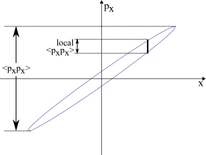
Figure 1: The local momentum $\mathbf{\Sigma}$-matrix describes the distribution of momentum in a small spatial element of the bunch.

The local momentum spread is obtained via

$$\mathbf{\Sigma}_{lpp}\equiv\left<\bar{p}_{li}\bar{p}_{lj}\right>=\mathbf{\Sigma}_{pp}-\mathbf{\Sigma}_{xp}^{T}\mathbf{\Sigma}_{xx}^{-1}\mathbf{\Sigma}_{xp}\textrm{,}$$ (3)

where $\mathbf{\Sigma}_{pp}\equiv\left<\bar{p}_{i}\bar{p}_{j}\right>$, $\mathbf{\Sigma}_{xx}\equiv\left<\bar{x}_{i}\bar{x}_{j}\right>$, and $\mathbf{\Sigma}_{xp}\equiv\left<\bar{x}_{i}\bar{p}_{j}\right>$.

$\mathbf{\Sigma}_{lpp}$ is symmetric and positive-definite and can be decomposed as

$$\mathbf{\Sigma}_{lpp}=\mathbf{R}\mathbf{G}\mathbf{R}^{T}\textrm{,}$$ (4)

where $\mathbf{G}$ is a diagonal matrix of the eigenvalues of $\mathbf{\Sigma}_{lpp}$ and the columns of $\mathbf{R}$ are the eigenvectors. The eigenvalues are denoted $u_{1}$, $u_{2}$, $u_{3}$. Note that $\mathbf{R}^{T}=\mathbf{R}^{-1}$.

$\left<\mathbf{\delta w}^{2}\right>$ is obtained from

$$\left<\delta w_{1}^{2}\right> = g_{2}+g_{3}-2g_{1}\textrm{,}$$ (5)

$$\left<\delta w_{2}^{2}\right> = g_{1}+g_{3}-2g_{2}\textrm{,}$$ (6)

$$\left<\delta w_{3}^{2}\right> = g_{1}+g_{2}-2g_{3}\textrm{,}$$ (7)

where

$$g_{1} = g\left(u_{1},u_{2},u_{3}\right)\textrm{,}$$ (8)

$$g_{2} = g\left(u_{2},u_{1},u_{3}\right)\textrm{,}$$ (9)

$$g_{3} = g\left(u_{3},u_{1},u_{2}\right)\textrm{,}$$ (10)

and

$$g\left(a,b,c\right)=\\ \int_{0}^{\pi/2}\frac{2a\sin^{2}s\cos s}{\sqrt{\left(\sin^{2}s+\frac{a}{b}\cos^{2}s\right)\left(\sin^{2}s+\frac{a}{c}\cos^{2}s\right)}}ds\textrm{.}$$ (11)

$g_{1}$, $g_{2}$, and $g_{3}$ are analogous to the temperatures of the three normal modes of the bunch.

$c_{I}$ is defined as

$$c_{I}=\frac{r_{e}^{2}N_{e}\Delta s}{4\pi\gamma^{4}\epsilon_{a}\epsilon_{b}\epsilon_{c}}C_{\Lambda}\textrm{,}$$ (12)

where $\epsilon_{a}$, $\epsilon_{b}$, and $\epsilon_{c}$ are the normal mode emittances of the beam, and the Coulomb logarithm $C_{\Lambda}$ will be defined in the next section. $N_{e}$ is the number of particles in the bunch, $r_{e}$ is the classical electron radius, $\gamma$ is the relativistic factor, and $\Delta s$ is the length of the region over which particles interact.

II.1 Coulomb logarithm

The Coulomb log, $C_{\Lambda}$, appears in the integration of the Rutherford scattering cross-section over all scattering angles. The integral diverges for small scattering angles, which correspond to large impact parameters. This requires the introduction of a largest impact parameter cutoff. We follow the prescription by Kubo and Oide Kubo and Oide (2001) and use the smaller of the mean inter-particle distance and the smallest beam dimension as the maximum impact parameter,

$$b_{max}=\min\left(n^{-1/3},\sigma_{x},\sigma_{y},\gamma\sigma_{z}\right),$$ (13)

where $n$ is the particle density in the bunch frame,

$$n=\frac{N_{e}}{\left(4\pi\right)^{3/2}\sigma_{x}\sigma_{y}\gamma\sigma_{z}}.$$ (14)

As for the largest scattering angle (smallest impact parameter), both Piwinski and Bjorken-Mtingwa assume that $\theta_{max}=\pi/2$. It was suggested in Raubenheimer (1994) that scattering events which occur less frequently than once per particle per radiation damping time should be excluded from the calculation of the IBS rise time. This is because such events do not occur frequently enough for the central limit theorem to apply and therefore do not contribute to the Gaussian core of the beam. Such infrequent events will generate non-Gaussian tails. It is the size of the Gaussian core that we can measure, so for comparison with the data, we exclude contributions to the tails.

The canonical momentum of a particle in an electron/positron storage ring is the sum over a history of momentum kicks that occur whenever the particle radiates a photon. The photon carries away some transverse momentum, but the emission event can also increase the transverse momentum of the particle if the photon is emitted in a region of finite dispersion. The overall effect of the emission event on the particle’s momentum depends on the action, angle, and local optics where a photon is emitted. Because photon emission is stochastic and occurs at random points along the particle’s trajectory, the kicks are also stochastic. According to the central limit theorem, the momenta of particles in a bunch will be normally distributed in the absence of IBS. In the presence of IBS, the distribution consists of a core which is close to Gaussian, along with non-Gaussian tails.

The amount of transverse momentum taken away by the radiated photon tends to be larger for particles with a larger transverse momentum. This leads to damping and results in an equilibrium distribution of momenta, rather than unbounded momentum diffusion. Perturbations to particle motion damp exponentially with a characteristic radiation damping time. Within one damping time, a large number of stochastic photon emission events occur. For CesrTA, about $20\times 10^{6}$ photons are emitted per particle per damping time.

Similarly, there are a large number of small-angle intrabeam scattering events that likewise excite oscillations. These IBS events increase the width of the momentum distribution. However, very few large-angle scattering events occur per damping time.

A particle with velocity $v$, traveling through a gas with density $\rho$, and an interaction cross-section $\sigma$, will undergo scattering events at a rate $1/\tau=\rho v\sigma$. Writing $\sigma=\pi b^{2}$, where $b$ is the effective impact parameter yields

$$\frac{1}{\tau}=\pi\rho vb^{2}\textrm{.}$$ (15)

For non-relativistic Coulomb scattering, the impact parameter is related to the scattering angle $\psi$ by

$$b=\frac{r_{e}}{2\bar{\beta}^{2}}\cot\frac{\psi}{2}$$ (16)

where $\bar{\beta}c$ is the velocity of the particles in their center-of-momentum frame. Substituting Equation (16) into (15) gives the rate in the lab frame at which particles are scattered into angles less than or equal to $\psi$:

$$\frac{1}{\tau}=\frac{1}{\gamma}\frac{\pi\rho cr_{e}^{2}}{4\gamma^{3}\left(\epsilon\gamma_{a}\right)^{\frac{3}{2}}}\cot^{2}\frac{\psi}{2}$$ (17)

where $\gamma\sqrt{\epsilon\gamma_{a}}$ has been used for $\bar{\beta}$, $\epsilon$ is the geometric emittance, and $\gamma_{a}$ is the $a$-mode Twiss $\gamma$. The relevant beam parameters for CesrTA are shown in Table 2.

Table 2: Nominal conditions for a bunch with $6.4\times 10^{10}$ particles.

Beam Energy $\gamma$	$4080$
Average Density $\rho$	$4.2\times 10^{21}$ part/m3
Twiss $\gamma_{x}$	$0.51$ m-1
Emittance $\epsilon_{a}$	$3.0$ nm-rad

The rate of scattering events, $\Gamma_{s}$, in units of radiation damping time, $\Gamma_{r}$, as a function of maximum scattering angle is shown in Fig. 2a. The tail-cut excludes those events which occur less than once per radiation damping period. A measure of the sensitivity to the cutoff is illustrated in Fig. 2b. The calculated equilibrium beam size is shown for a range of two orders of magnitude of the cutoff. The data shown is the same as plotted in Fig. 9a.

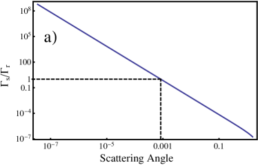
(a)

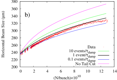
(b)

Figure 2: LABEL:sub@fig:tail-cut-rates:a Events which occur less than once per damping time are excluded from the calculated growth rate. LABEL:sub@fig:tail-cut-rates:b Equilibrium beam size calculations assuming different cut-offs.

The tail-cut consists of restricting the calculation of the IBS growth rate to include only those events which occur at least once per particle per damping period. Events which occur less frequently than once per damping period generate lightly populated non-Gaussian tails that do not contribute to the Gaussian core. It is the Gaussian core that we can measure and that is important when determining the brightness of a light source or luminosity in a collision experiment.

The tail-cut is applied by setting the minimum impact parameter as

$$b_{min}=\sqrt{\frac{1}{n\pi\tau_{b}\nu}},$$ (18)

where $\tau_{b}$ is the longest damping time in the bunch frame and $\nu$ is the average particle velocity in the bunch frame. If $\epsilon_{a}$ is greater than $\epsilon_{b}$ and $\frac{\sigma_{p}\sigma_{z}}{\gamma^{2}}$, then $\nu\approx c\gamma\sqrt{\frac{\epsilon_{a}}{\beta_{a}}}$.

The computed IBS growth rate is directly proportional to the Coulomb log and is expressed as the logarithm of the maximum impact parameter over the minimum,

$$C_{\Lambda}=\log\frac{b_{max}}{b_{min}}.$$ (19)

In hadron and ion machines, such as the Tevatron and RHIC, the damping time is very long and there are enough of even the very large-angle scatters to populate a Gaussian distribution. A tail-cut does not significantly affect the calculated IBS distributions for those machines. However, for machines with strong damping, such as lepton storage rings, very few large-angle scattering events occur per damping time, and applying the tail-cut is essential to reliably computing the equilibrium distribution of the Gaussian core of the bunch. In CesrTA, applying the tail-cut significantly changes the calculated growth rate. With the tail-cut, the average Coulomb log in CesrTA at $1.6\times 10^{10}$ particles/bunch is $9.4$. Without the tail-cut, that is, if we assume that the maximum scattering angle is $90^{\circ}$, the average Coulomb log is $17.6$.

II.2 Monte Carlo IBS Simulations

In addition to the analytic IBS calculations discussed above, we have developed a Monte Carlo simulation based on Takizuka and Abe’s plasma collision model Takizuka and Abe (1977). An ensemble of $2000$ particles representing the bunch distribution is tracked element-by-element using the Bmad standard tracking methods Sagan (2006). We use an analytic model of the damping wiggler field, which is based on a fit to a finite element calculation Sagan et al. (2003a). Tracking through wigglers is by symplectic integration.

At each element, the ensemble is converted from canonical to spatial coordinates and boosted into its center of momentum frame where the particles are non-relativistic. Then Takizuka and Abe’s collision model is applied:

1. The bunch is divided into cells. This enforces locality.

2. Particles in each cell are paired off. Each particle undergoes only one collision.

3. The change in the momentum of the pair is calculated, taking into account their relative velocities and the density of particles in the cell.

The ensemble is then boosted back to the lab frame and transformed back into canonical coordinates.

Note that this is not a Monte Carlo simulation of individual scattering events. Such a simulation would require the calculation of $\frac{N!}{2}$ scattering events per element and is not computationally feasible. Takizuka and Abe’s formalism calculates the expectation value of the change in the momentum of a test particle traveling through a “wind” of nearby particles. The relative velocity of the paired particles determines the velocity vector of the wind. The rate of change of the particle momentum due to scattering events is assumed to be constant through the length of the element.

A log term corresponding to the Coulomb log appears in Takizuka and Abe’s formalism. The calculation of the expectation value of the change in the momentum of the particles assumes many small-angle scattering events. This method of Monte Carlo simulation is subject to the central limit theorem and tail-cut in the same way as the analytic calculations.

II.3 Potential Well Distortion (PWD)

The bunch interacts with structures in the vacuum system, resulting in wake fields that act back on the bunch. One consequence of this is a voltage gradient along the length of the bunch. Particles at the head of the bunch lose energy to the vacuum system. Part of this energy is reflected back to the tail of the bunch, effectively transferring energy from the head of the bunch to the tail. In machines that operate above transition, particles with less energy move ahead relative to the reference particle, and those with more energy move back. The result is bunch lengthening. The amount of lengthening is sensitive to the total bunch charge, but not to the transverse dimensions of the bunch.

Energy that is reflected back into the bunch does not change the total energy of the bunch and is referred to as the inductive ($L$) or capacitive ($C$) part of the impedance. Energy absorbed by the vacuum system does change the total energy of the bunch and is referred to as the resistive part of the impedance ($R$).

In the general case, the impedance is frequency dependent. Here, the effect of potential well distortion is approximated as a current-dependent RF voltage. The effective RF voltage is Billing (1980)

$$V\left(\tau\right)=V_{rf}\cos\left(\omega\tau+\phi\right)+RI_{b}\left(\tau\right)+L\frac{dI_{b}\left(\tau\right)}{d\tau},$$ (20)

where $\tau$ is relative to the bunch center. The resistive impedance $R$ tends to shift the synchronous phase but does not contribute to lengthening. The inductive part $L$ changes the Gaussian profile of the bunch, leading to real bunch lengthening.

In principle, there is also a capacitive part to the impedance. Its effect is to shorten the bunch. In CesrTA, only bunch lengthening is observed. This is because the inductive term in the overall impedance is much larger than the capacitive. Hence, the reactive part of the impedance is modeled as entirely inductive. In theory, the inductive, capacitive, and resistive parts of the impedance could each be determined from the shape of the longitudinal profile of the bunch. However, our measurements are not detailed enough to determine if a capacitive part of the impedance is counteracting the inductive part.

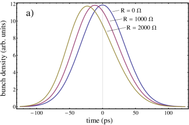
(a)

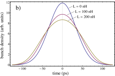
(b)

Figure 3: Effect of LABEL:sub@fig:rl-pwd:L inductive and LABEL:sub@fig:rl-pwd:R resistive parts of the longitudinal impedance on the longitudinal profile of the bunch.

A derivation of PWD based on Vlassov theory results in a differential equation for the longitudinal profile of the bunch Billing (1980),

$$\frac{\partial\psi}{\partial\tau}=-\frac{eE_{0}\psi}{\sigma_{E}^{2}\alpha T_{0}}\left(\frac{V_{rf}\cos\left(\omega\tau+\phi\right)+QR\psi-U_{0}}{1+\frac{eE_{0}QL\psi}{\sigma_{E}^{2}\alpha T_{0}}}\right),$$ (21)

where $E_{0}$ is the beam energy, $\sigma_{E}$ is energy spread, $\alpha$ is momentum compaction, $T_{0}$ is the period of the ring, $V_{rf}$ is the total RF cavity voltage, $\omega$ is the RF frequency, $\phi$ is the phase of the reference particle with respect to the RF, $Q$ is the bunch charge, $U_{0}$ is the energy lost per particle per turn, $R$ is the resistive part of the longitudinal impedance, and $L$ is the inductive part of the longitudinal impedance. $\psi\left(\tau\right)$ is the longitudinal profile of the bunch. Equation (21) is used to compute the effect of various resistive and inductive impedances on the longitudinal profile of the bunch. The results are shown in Fig. 3.

We have incorporated the effect of PWD in our analytic model of IBS. Equation (21) is used to compute bunch length, including the energy spread resulting from intrabeam scattering. Comparing the measured bunch length versus current data to the simulation result, $L$ is determined to be $25.9^{+18.7}_{-17.2}$ nH for positrons and $21.1^{+15.3}_{-14.5}$ nH for electrons. Our bunch length predictions are largely insensitive to $R$, and we use the published value of $1523$ $\Omega$ given by Holtzapple et al. Holtzapple et al. (2000). At the time of this writing, PWD has not been implemented in the Monte Carlo simulation.

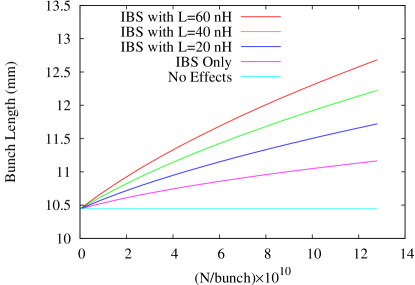
Figure 4: Simulated effect on bunch length of PWD in combination with IBS.

As shown in Fig. 3, resistive impedance has a negligible effect on the length of the longitudinal profile, whereas the inductive impedance $L$ distorts the Gaussian profile and generates bunch lengthening. Figure 4 shows the contribution of the potential well distortion to the bunch length assuming various values for the inductive impedance.

The current-dependent energy spread in CesrTA is determined by measuring the dependence of the horizontal beam size on the horizontal dispersion at the instrument source point. The dispersion is varied with the help of a closed dispersion bump around the source-point. The horizontal beam size is measured under two sets of conditions as the number of particles in a single bunch decays from $1.3\times 10^{11}$ down to $2.4\times 10^{10}$. Horizontal dispersion is $2.28$ cm in the first set of conditions, and $22.1$ cm in the second. The measured energy spread is $\sigma_{E}/E=\left(8.505\pm 0.314\right)\times 10^{-4}$ and is independent of current within the measurement uncertainty. The design value of the fractional energy spread as determined using the standard radiation integrals is $8.129\times 10^{-4}$. There is no evidence of a microwave instability, which would appear as an energy spread that increases with current above some threshold current.

II.4 Projected Beam Sizes

Beam sizes from the simulations are obtained from the $\left<xx\right>$, $\left<yy\right>$, and $\left<zz\right>$ elements of the $6\times 6$ beam envelope matrix. These are evaluated at the instrumentation source-points. The beam sizes obtained by this method are the projections of the beam into the horizontal, vertical, and longitudinal dimensions and are the bunch profiles actually seen by the instrumentation. This method naturally takes into account arbitrary coupling among the 6 normal mode phase-space coordinates of the bunch.

II.5 Method Comparison

In addition to Kubo and Oide’s method, two other commonly used methods for calculating IBS growth rates are one by Bjorken and Mtingwa Bjorken and Mtingwa (1983) and a version of Piwinski’s original derivation that includes derivatives of the lattice optics Piwinski (1974). Figure 5 shows the equilibrium beam sizes versus current calculated using each of the three methods.

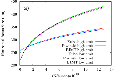
(a)

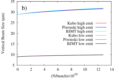
(b)

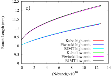
(c)

Figure 5: Comparing LABEL:sub@fig:Method-Comp-horiz Horizontal, LABEL:sub@fig:Method-Comp-vert vertical, and LABEL:sub@fig:Method-Comp-long longitudinal beam size versus current for Kubo’s, Piwinski’s, and the Bjorken-Mtingwa (BJMT) IBS formalisms. The high emittance lattice has $\epsilon_{x0}=4.6$ nm$\cdot$rad, $\epsilon_{y0}=14.3$ pm$\cdot$rad, and $\sigma_{z0}=10.0$ mm. The low emittance lattice has $\epsilon_{x0}=2.8$ nm$\cdot$rad, $\epsilon_{y0}=1.5$ pm$\cdot$rad, and $\sigma_{z0}=10.3$ mm.

We treat the Coulomb log the same way in each method and apply the tail-cut. Applying the tail-cut to Piwinski’s original method requires modifying the derivation so that the minimum and maximum scattering angles can be set as parameters.

Bjorken and Mtingwa’s and Piwinski’s methods are based on Twiss parameters. We use normal mode Twiss parameters in place of horizontal, vertical, and longitudinal Twiss parameters when evaluating either formalism. The growth rates given by the formulas are applied to the normal mode emittances.

These calculations suggest that, provided the Coulomb log is treated the same, the three most general IBS formalisms predict similar equilibrium beam sizes. For the studies shown here, transverse coupling is not strong enough to significantly impact the IBS growth rates.

III Current-Dependent Tune Shift

A current-dependent shift of the coherent tune is observed in CesrTA. At $2.1$ GeV, the vertical shift was measured to be $-0.505\pm 0.006$ kHz/mA. The horizontal shift was measured to be $-0.072\pm 0.006$ kHz/mA. ($1$ kHz corresponds to a change in fractional tune of $0.0026$.) The synchrotron tune has been measured versus current, and no shift was observed. These tune shifts are relevant to IBS studies because the beam size will in general depend on proximity of the coherent tune to resonance lines in the tune plane. Preparation for IBS studies includes identifying a region of the tune plane where the effect of resonance lines is minimized for the range of currents to be explored. The tune plane is scanned with direct measurement as well as tracking simulation. The experimental tune scans are performed by recording the beam sizes as the tune is varied by adjusting quadrupole strengths.

Figure 6 shows the measured dependence of vertical and horizontal coherent tunes on bunch current. The betatron frequencies are measured via a pair of spectrum analyzers connected to beam position monitor (BPM) buttons.

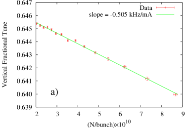
(a)

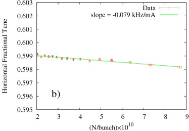
(b)

Figure 6: Fractional coherent tune versus current for LABEL:sub@fig:68-Tune-Data:v the vertical and LABEL:sub@fig:68-Tune-Data:h the horizontal plane. The resolution of the measurement is $10^{-4}$. The revolution frequency is $390.1$ kHz.

Figure 7 shows a simulated tune scan. The color scale shows the rms value of the vertical-like normal mode action $J_{b}$ of a particle tracked for $2000$ turns, normalized by its initial value $J_{b0}$. The thin lines are analytic calculations of the form $rQ_{x}+sQ_{y}+tQ_{z}=n$. The labels are of the form $\left(r,s,t,n\right)$. Amplitude-dependent tune-shift causes the resonance lines in the simulation to be offset from the analytic calculations. The initial action $J_{b0}$ of the tracked particle is set to be about ten times the equilibrium emittance. The yellow line shows the range of coherent tune spanned as a bunch decays from $1.3\times 10^{11}$ particles to $1.6\times 10^{9}$ particles. The upper right hand point is the zero current tune.

The simulated and experimental tune scans are generally only in approximate agreement. The lower order resonances, such as $\left(1,-1,-1,0\right)$, tend to be much broader in the experimental tune scan. The higher order resonances seen in the simulated scan do not appear in the experimental scan. The working points for the IBS measurements are chosen with consideration of both the simulated and measured tune scans; further adjustments are often needed based on machine behavior.

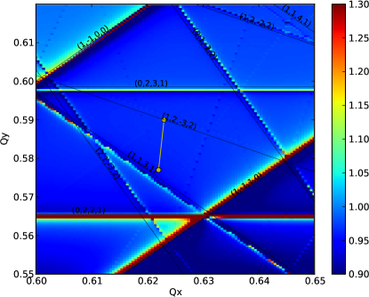
Figure 7: Simulated tune scan based on a lattice model that includes magnet misalignments and corrector magnet settings determined according to our emittance tuning procedure. The yellow line shows how the coherent tunes increase as a bunch decays from $1.3\times 10^{11}$ down to to $1.6\times 10^{9}$ particles.

IV Simulation Lattices

An element-by-element description of CesrTA is used for the analytic and tracking calculations shown here. This description includes quadrupoles, sextupoles, bends, steerings, skew quadrupole correctors, wigglers, and RF cavities. Systematic multipoles are included for those sextupoles which have skew quadrupole or vertical steering windings. We use an analytic model of the damping wiggler field, which is based on a fit to a finite element calculation Sagan et al. (2003b). Tracking through wigglers is by symplectic integration.

The vertical IBS rise time depends on the dispersion. However, vertical dispersion is zero for an ideal flat ring. Vertical dispersion is included in our analytic IBS calculations by introducing $yz$ coupling into the 1-turn transfer matrix. This is done at each element by augmenting the 1-turn transfer matrix before utilizing it in the analytic IBS calculation. The transfer matrix $\mathbf{T}$ is replaced with with $\mathbf{\tilde{T}}$, where $\mathbf{\tilde{T}}=\mathbf{T}\mathbf{W}$, and

$$\mathbf{W}=\begin{pmatrix}1&0&0&0&0&0\\ 0&1&0&0&0&0\\ 0&0&1&0&0&-\tilde{\eta}_{y}\\ 0&0&0&1&0&-\tilde{\eta}^{\prime}_{y}\\ 0&0&\tilde{\eta}_{y}^{\prime}&-\tilde{\eta}_{y}&1&0\\ 0&0&0&0&0&1\end{pmatrix}.$$ (22)

This transformation preserves the symplecticity of the transfer matrix. $\tilde{\eta}_{y}$ and $\tilde{\eta}^{\prime}_{y}$ are dispersion-like quantities. An ideal lattice modified according to the above prescription with $\tilde{\eta}_{y}=0.01$ m and $\tilde{\eta}^{\prime}_{y}=0.002$ has an rms vertical dispersion of $10.9$ mm and a vertical IBS risetime similar to that of a lattice with an rms vertical dispersion of $10$ mm.

The vertical dispersion in CesrTA is measured to be less than $15$ mm. The upper bound is limited by the resolution of our measurement technique. The coupling is determined by direct measurement to be $\bar{C}_{12}<0.003$, using an extended Edwards-Teng formalism Sagan and Rubin (1999). This amount of coupling is negligible, and the simulation assumes no transverse coupling.

The analytic simulation takes the measured low current horizontal and vertical beam sizes and bunch length as input parameters and computes the current dependence. The horizontal emittance used in the calculation is chosen to match the measured near zero current emittance. The vertical emittance is also set to agree with the measurement extrapolated to zero current. (The vertical emittance of the design simulation lattice is zero.) The energy spread and bunch length used in the simulation are obtained by evaluating the standard radiation integrals.

The Monte Carlo simulation includes photon emission and so requires a realistic vertical dispersion function. This is generated by applying a distribution of misalignments to the ideal lattice, then correcting the phase advance, coupling, orbit, and vertical dispersion according to the same procedure that is applied to CesrTA low-emittance tuning Shanks (2011). The magnitude of the misalignments is set such that the zero current vertical emittance is roughly $15$ pm-rad.

V Experiment

For measurements of intrabeam scattering, we load a specific lattice configuration into the storage ring, which includes beam energy, working point, and RF voltage. The orbit, betatron phase, transverse coupling, and dispersion are measured at each of the $100$ beam position monitors around the ring and then corrected to match the design. The phase and coupling data is derived from turn by turn position measurements at each of the beam position monitors for a resonantly excited beam Sagan et al. (2000). The measurement of betatron phase and coupling takes $10$ seconds, with phase reproducibility of order $0.05$ deg and $\bar{C}_{12}$ reproducibility of $0.002$. The dispersion is determined by directly measuring the dependence of closed orbit on beam energy (RF frequency). The machine model is fit to the measured phase, coupling and dispersion by varying all $100$ quadrupoles, $25$ skew quadrupole, and $55$ vertical steering correctors. The machine optics are forced to match the design by loading the fitted magnet changes with opposite sign. The procedure typically converges in a few iterations. An example measurement of the optical functions after correction and just prior to an IBS run is shown in Fig. 8. The machine is tuned for minimum vertical emittance according to the algorithm given in Shanks (2011). For experiments requiring a larger beam size, the vertical emittance is increased by adjusting a closed coupling and vertical dispersion bump that propagates vertical dispersion through the wigglers.

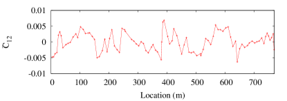
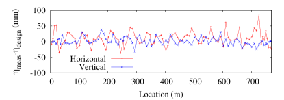
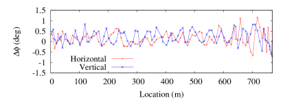
Figure 8: Top: Measured transverse coupling at each beam position monitor after correction. $\bar{C}_{12}$ is the ratio of the normalized amplitude of vertical to horizontal motion when the beam is driven at the $a$-mode (horizontal) tune. Middle: Measured dispersion error with respect to design $\left(\eta_{measured}-\eta_{design}\right)$. Bottom: The residual betatron phase error $\left(\phi^{h,v}_{measured}-\phi^{h,v}_{design}\right)$. A $1^{\circ}$ rms phase error corresponds to a $\sim 2$% $\beta$ error.

A single bunch of about $1.6\times 10^{11}$ particles ($10$ mA) is allowed to decay. The measurements include horizontal and vertical beam sizes, streak camera measurements of the longitudinal profile, and tunes in all three dimensions. The beam current decays from $10$ mA to $1$ mA in about $20$ minutes. The short beam lifetime is due to Touschek scattering; below $1$ mA, where the charge density is considerably smaller, the beam lifetime improves significantly. In the interest of time, a large-amplitude pulsed orbit bump is used to scrape particles out of the beam in $0.25$ mA decrements. The discontinuities in the data at bunch charge $<2\times 10^{10}$ particles correspond to the regime where beam is scraped out.

IBS measurements are taken during dedicated periods of CesrTA operation. The IBS measurements in 2011 led us through iterative improvements in our understanding of how to operate the accelerator and how to measure IBS effects. Improvements on the accelerator side included a better understanding of the tunes and the selection of the working point (tunes as determined by lattice optics), a better understanding of the coupling and its impact on the measurements, and the development of more exact procedures for establishing the desired machine configuration. Improvements to the instrumentation included the implementation of beam size measurements for both electrons and positrons and the development of more accurate and robust analysis software. The data presented here were taken during the April 2012 CesrTA run. The measurements in December 2012 and April 2013 corroborate and expand on the April 2012 run and have been published in Ehrlichman et al. (2013a) and Ehrlichman et al. (2013b).

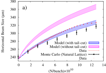
(a)

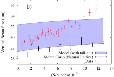
(b)

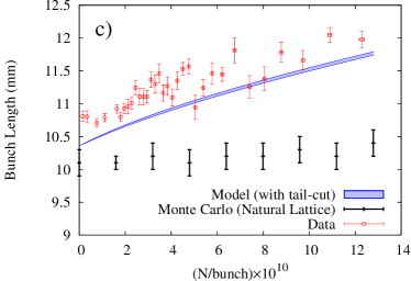
(c)

Figure 9: LABEL:sub@fig:4B-Methods-horiz Horizontal, LABEL:sub@fig:4B-Methods-vert vertical, and LABEL:sub@fig:4B-Methods-long longitudinal beam size versus current for $e^{+}$ bunch in conditions tuned for minimum vertical emittance.

Figure 9 shows the data from a positron bunch in conditions tuned for minimum vertical emittance. Analytic results from the $\mathbf{\Sigma}$-matrix formalism described in Sec. II and the Monte Carlo simulation described in Sec. II.2 are shown along with the data. Some of the error bars in Fig. 9 are below the resolution of the plot. The approximate statistical uncertainties at high current are shown in Table 3.

Table 3: Approximate statistical uncertainties at high current.

Measurement	Uncertainty
Current (horiz. binning)	$0.3$%
Current (bunch length binning)	$0.9$%
Horizontal Size	$0.2$%
Bunch Length	$1.0$%
Vertical Size	$0.2$%

The systematic uncertainty in the measured horizontal beam size is about $2$%, and is due to vibration of optical elements and horizontal beam motion. The systematic uncertainty in the vertical measurement is about $\pm 2$ $\mu$m and is dominated by our understanding of the x-ray optics and detector.

The accuracy of the simulation is limited by the ambiguity of the Coulomb log and limited knowledge of the zero current vertical beam size of the machine. The simulation result shown here follows the usual convention for the tail-cut of $1$ event/damping time as the cutoff.

The $\mathbf{\Sigma}$-matrix IBS simulation is run twice, once with a zero current vertical emittance that extends to the bottom range of the measurement systematic uncertainty, and once that extends to the upper range of the measurement systematic uncertainty. The shaded region is the area between those two results. This serves two purposes. First, it reflects the systematic uncertainty in the vertical beam size measurements. Second, it gives the reader an idea of how the horizontal simulation result depends upon particle density as determined by the vertical beam size.

The zero current vertical emittances that bound the data in Fig. 9b are $17.9$ pm and $25.1$ pm. The shaded regions of 9a and 9c show how the horizontal and vertical simulation results change as the zero current vertical emittance is varied from the lower bound to the upper bound.

The measured zero current horizontal emittance, which is an input parameter to the simulation, is $3.8$ nm-rad. For the bunch length and energy spread, we use the values calculated from the radiation integrals.

The simulation uses a perfectly aligned CesrTA lattice. Vertical dispersion is included by modifying the 1-turn transfer matrix with $\mathbf{W}$ before passing it to the IBS rise-time calculation. $\tilde{\eta}$ is set to $10$ mm.

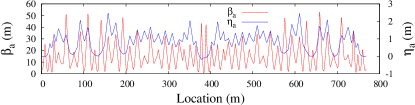
Figure 10: CesrTA design $a$-mode (horizontal-like) $\beta$ and dispersion $\eta$.

The horizontal emittance increases from $3.8$ nm-rad at low current ($<1.5\times 10^{9}$ particles/bunch) to $10.4$ nm-rad at $1.3\times 10^{11}$ particles/bunch. The reason for the relatively large horizontal blow-up is the large horizontal dispersion in CesrTA. The lattice functions $\beta_{a}$ and $\eta_{a}$ are shown in Fig. 10. The rms horizontal dispersion, $\eta_{a}$, is $1.0$ m and peaks at $2.5$ m. For comparison, the rms vertical dispersion is less than $15$ mm.

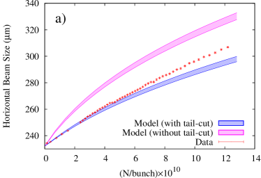
(a)

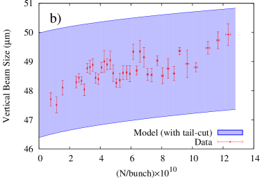
(b)

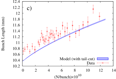
(c)

Figure 11: LABEL:sub@fig:53-Data-horiz Horizontal, LABEL:sub@fig:53-Data-vert vertical, and LABEL:sub@fig:53-Data-long longitudinal beam size versus current for $e^{+}$ bunch with increased zero current vertical emittance.

In Fig. 11 the zero current vertical emittance of the bunch was increased by propagating vertical dispersion through the damping wigglers with the help of a closed coupling and dispersion bump. The larger vertical beam size decreases the particle density, which in turn reduces the amount by which IBS blows up the horizontal beam size. The zero current horizontal emittance is $3.7$ nm-rad. The zero current vertical emittances that bound the data are $51.6$ pm and $59.9$ pm.

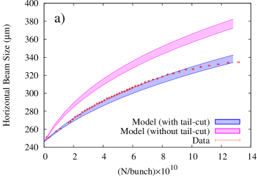
(a)

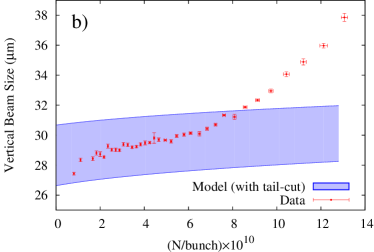
(b)

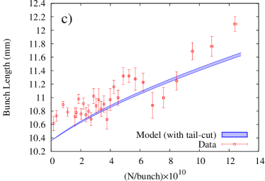
(c)

Figure 12: LABEL:sub@fig:68-Data-horiz Horizontal, LABEL:sub@fig:68-Data-vert vertical, and LABEL:sub@fig:68-Data-long longitudinal beam size versus current for $e^{-}$ bunch in conditions tuned for minimum vertical emittance.

IBS theory is species-independent. Measurements of both $e^{-}$ and $e^{+}$ can help identify machine and instrumentation systematics and distinguish IBS from species-dependent beam physics such as electron cloud and ion effects. Figure 12 shows data from an electron bunch in conditions tuned for minimum vertical emittance. The measured horizontal emittance is $4.3$ nm-rad at zero current and $8.2$ nm-rad at $4.8\times 10^{10}$ particles/bunch. The zero current vertical emittances that bound the data are $16.9$ pm and $22.4$ pm.

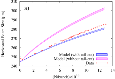
(a)

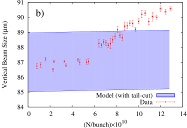
(b)

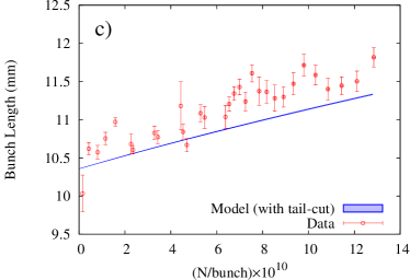
(c)

Figure 13: LABEL:sub@fig:6B-Data-horiz Horizontal, LABEL:sub@fig:6B-Data-vert vertical, and LABEL:sub@fig:6B-Data-long longitudinal beam size versus current for $e^{-}$ bunch with increased zero current vertical emittance.

Data from an e^- run where the vertical emittance was increased are shown in Fig. 13. The horizontal emittance is $4.2$ nm-rad at zero current and $5.5$ nm-rad at $4.8\times 10^{10}$ particles/bunch. The vertical emittances that bound the data are $172$ pm and $188$ pm.

Figure 14 shows the combined data from the two $e^{-}$ and two $e^{+}$ data sets.

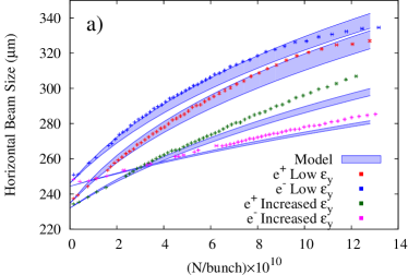
(a)

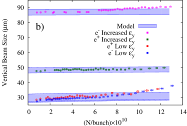
(b)

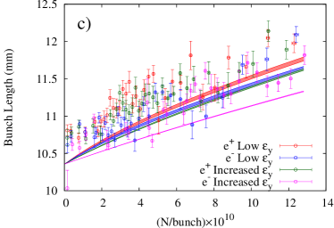
(c)

Figure 14: Aggregated LABEL:sub@fig:agg-Data-h Horizontal, LABEL:sub@fig:agg-Data-v vertical, and LABEL:sub@fig:agg-Data-l longitudinal data comparing $e^{+}$ and $e^{-}$ in minimum emittance conditions and conditions where the zero current vertical emittance was blown up using closed coupling and dispersion bumps.

VI Discussion

VI.1 Data

IBS effects are most evident in the horizontal dimension, where large horizontal dispersion leads to significant blow-up. In comparison, IBS is not a strong effect in the vertical. This is because the vertical dispersion is so small. The direct transfer of momentum from the horizontal to the vertical by IBS is small at high energy.

The amount of the blow-up can be controlled by varying the vertical emittance, and thus the particle density. The simulations show bunch lengthening due to IBS, but we are unable to distinguish IBS lengthening from potential well distortion in our measurements.

An interesting anomaly we have encountered is the behavior of the vertical beam size at high currents. The effect is seen in Figs. 9b and 12b above $8\times 10^{10}$ particles/bunch. We observe that vertical beam size plotted versus current increases with positive curvature. Much more severe cases of this blow-up have been observed during the machine studies. We find that adjusting betatron and synchrotron tunes during experiments affects the blow-up, but in a somewhat unpredictable way. The blow-up is observed in both electron and positron beams.

The observed blow-up in the vertical does not appear to be an instrumentation effect because when the vertical size blows up, the horizontal size drops. This is because the blow-up in the vertical reduces the particle density, which reduces the IBS effect in the horizontal.

At high current, the vertical beam centroid position over $32768$ turns was recorded using the xBSM. A fast Fourier transform of this data does not show a clear signal above background, so we cannot attribute the anomalous growth in vertical size to an instability. Adjustments to the corrected chromaticity did not impact the blow-up.

Measurements of coupling $\bar{C}_{12}$ at different bunch currents are shown in Fig. 15. There is no evidence of significant current-dependent transverse coupling.

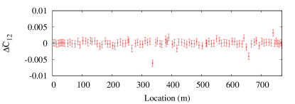
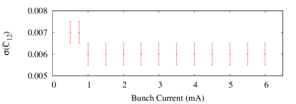
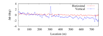
Figure 15: Top: Difference in transverse coupling at $6$ mA vs $0.8$ mA single bunch current measured at each BPM. Middle: Current dependence of rms $\left(\sigma\right)$ of residual coupling of all $N$ BPMs where $\sigma^{2}=\frac{1}{N}\sum_{i=1}^{N=100}\left(\bar{C_{i}}_{12}\right)^{2}$. Bottom: Difference in betatron phase at $6$ mA vs. $0.8$ mA single bunch current. The downward trend in the vertical corresponds to the current dependent tune shift. $\beta$ is related to the phase advance from one BPM to the next. The fractional change in $\beta$ from $6$ mA to $0.8$ mA is less than $1$%.

The measured bunch length shown here is consistently about $0.5$ mm longer than the predicted value. Measurement results from December 2012 do not show this discrepancy. Between April and December 2012 the streak camera was realigned and the analysis software was improved. However, the evidence does not point to any particular instrumentation systematic.

VI.2 Theory

The presence of the Coulomb log is a well-known ambiguity in IBS theory as it requires the introduction of loosely defined cutoffs in the minimum and maximum scattering angle. The choice of one event per damping time as the boundary between multiple-event and single-event scattering is somewhat arbitrary. That said, the data shown here are in reasonable agreement with theory, suggesting that with implementation of the tail cut, the IBS theory is a reasonable model of performance for electron and positron machines. Furthermore, as shown in Fig. 2b, the theory gives a good description of the data even when the large angle cutoff used in the calculation is varied by more than an order of magnitude.

The theory used here is Kubo and Oide’s $\mathbf{\Sigma}$-matrix based IBS formalism. This model is a generalization of Bjorken and Mtingwa’s formalism that can handle arbitrary coupling of the horizontal, vertical, and longitudinal motion. It includes the tail-cut. Coupling in CesrTA for the experiments shown here was not large enough to noticeably impact the IBS growth rates. If coupling were significantly larger, then the predictions from Kubo and Oide’s method may diverge from those of Bjorken and Mtingwa’s method. Additional IBS studies with more strongly coupled beams are planned to investigate this regime.

VII Conclusion

We have presented data on intrabeam scattering in a high-intensity, wiggler-dominated, $e^{-}$/$e^{+}$ storage ring. Additional current-dependent effects, such as tune shift and potential well distortion, have been observed in the beams. An anomalous blow-up in the vertical dimension is seen at high current and requires further study.

This data has been compared to a generalized version of the Bjorken-Mtingwa formalism for calculating IBS effects. The results presented here suggest that, provided the tail-cut procedure is applied, existing IBS theory is an accurate predictor of machine performance in $e^{+}$/$e^{-}$ machines.

Further IBS studies at CesrTA include adjusting wiggler parameters to observe how the equilibrium emittance of an IBS-dominated beam depends on the damping time, measurements at $1.8$, $2.3$, and $2.5$ GeV, and measurements with different RF voltages. There are also plans to explore IBS in strongly coupled beams. Some of these studies have been completed and are documented in Ehrlichman et al. (2012) and Ehrlichman (2013).