Phase transitions in 3D loop models and the $CP^{n-1}$ sigma model

Abstract

We consider the statistical mechanics of a class of models involving close-packed loops with fugacity $n$ on three-dimensional lattices. The models exhibit phases of two types as a coupling constant is varied: in one, all loops are finite, and in the other, some loops are infinitely extended. We show that the loop models are discretisations of $CP^{n-1}$ $\sigma$ models. The finite and infinite loop phases represent, respectively, disordered and ordered phases of the $\sigma$ model, and we discuss the relationship between loop properties and $\sigma$ model correlators. On large scales, loops are Brownian in an ordered phase and have a non-trivial fractal dimension at a critical point. We simulate the models, finding continuous transitions between the two phases for $n=1,2,3$ and first order transitions for $n\geq 4$. We also give a renormalisation group treatment of the $CP^{n-1}$ model that shows how a continuous transition can survive for values of $n$ larger than (but close to) two, despite the presence of a cubic invariant in the Landau-Ginzburg description. The results we obtain are of broader relevance to a variety of problems, including $SU(n)$ quantum magnets in (2+1) dimensions, Anderson localisation in symmetry class C, and the statistics of random curves in three dimensions.

I Introduction

This paper is concerned with the statistical physics of a family of three-dimensional (3D) lattice models for completely-packed loops that have transitions between phases of two types: one in which there are only short loops, and another in which some loops are extended. These models and phase transitions are interesting from several perspectives, since loops play an important role in a variety of problems from classical statistical mechanics and are also central to simulations of quantum systems. Our aim is to identify continuum field theories that describe long-distance properties of the models, to pin down the relation to quantum problems, and to study the phase transitions using large-scale Monte Carlo simulations. We have previously described some of this work in outline.prl Here we present a full account as well as additional results.

The models we discuss are characterised by a loop fugacity $n$, which can be interpreted as the number of possible colourings for each loop, and by a coupling constant $p$, which controls the distribution of loop lengths; full definitions are given in Sec. II. A defining feature of loop models, in contrast to spin systems, is that the basic degrees of freedom are extended objects. We show in Sec. III, however, that the partition functions can be re-written in terms of local degrees of freedom living on the complex projective space $CP^{n-1}$ and in this way we identify the loop models as discretisations of $CP^{n-1}$ $\sigma$ models. In addition, a dictionary can be established, expressing correlation functions of the $\sigma$ models in terms of those of the loop models: most importantly, the two-point correlation function of the $\sigma$ model is related to the probability that two links of the lattice lie on the same loop. The short-loop phase therefore represents the disordered phase of the $\sigma$ model, while infinite loops encode long range order of the $\sigma$ model. The relationship between correlation functions carries implications for the geometry of loops: in particular, the physics of Goldstone fluctuations implies that loops in the ordered phase are Brownian at large distances, while at a critical point loops have a fractal dimension related to the correlation exponent $\eta$ of the $\sigma$ model.

Depending on the value of the loop fugacity, the loop models can be mapped to various problems in critical phenomena. Setting $n=1$, they represent an important class of classical phase transitions which (like percolation) are geometrical rather than thermodynamic in nature, in the sense that they are visible only in geometrical observables. In this correspondence, the loops represent line defects in an environment with quenched disorder. Examples include the zero lines of a random complex field, tricolour percolation cosmic strings, cosmic strings or optical vortices. dennis The loop models at $n=1$ also arise via exact mappings from network models for certain Anderson metal-insulator transitions. glr ; beamond cardy chalker At this value of $n$, the field theory must either be construed as a replica limit, or augmented with fermionic degrees of freedom and supersymmetry. The properties of such $\sigma$ models and their connection with loop models have been discussed recently for two-dimensional (2D) systems read saleur ; candu et al while in previous work we have studied 3D loop models at $n=1$ ortuno somoza chalker and their general relation to geometrical phase transitions. vortex paper

Remarkably, when $n$ is greater than one, the same 3D loop models can be mapped to quantum $SU(n)$ antiferromagnets in $(2+1)$ dimensions by considering an appropriate transfer matrix. The phase with long loops is then the Neel phase, and one with only short loops is a valence bond liquid in which spins dimerise without breaking lattice symmetries. Indeed, the models we discuss here are closely related to loop algorithms that have been developed for Monte Carlo simulation of quantum spin systems.QMCreviews ; troyer ; alet A feature specific to our three-dimensional lattice model is that, since the ‘time-like’ axis is microscopically equivalent to the two ‘space-like’ ones, at a continuous quantum phase transition the dynamical exponent value $z=1$ is guaranteed, rather than a matter for calculation. Loop models with ‘deconfined’ transitions to valence bond solid phases may also be constructed by introducing extra couplings, and will be discussed in a separate paper.interacting

Besides their appearance in computational algorithms for quantum antiferromagnets, loop models with $n>1$ have been examined previously in a variety of other contexts. The 2D $CP^{n-1}$ sigma model has been simulated both by using the connection between $SU(n)$ magnets in $(1+1)$ dimensions and classical $\sigma$ models in $2$ dimensions,wiese05 and by means of a loop representation different from the one we describe here.wolff strong coupling Separately, there have been detailed studies of the properties of loops that arise in the description of some frustrated classical antiferromagnets,jaubert ; sondhi and of cycles that occur in statistical problems involving random permutations.schramm ; ueltschi

Loop models can be studied efficiently using Monte Carlo techniques, and we use simulations both as a check on our identification of them with $\sigma$ models and to investigate the phase transitions: results are presented in Sec. V. As a test we examine critical phenomena at $n=2$: the $CP^{1}$ model is known to be equivalent to the ${O}(3)$ (or classical Heisenberg) model, and our results are consistent with previous high precision investigationsO(3) numerics of that universality class. Moving beyond this check, an important basic question concerns the nature of the transition for general $n$. For $n>2$, Landau theory allows a cubic invariant, implying discontinuous ordering. We show, however, in Sec. IV, using an expansion around $n=2$ and dimension $d=4$, that fluctuations lead to a continuous transition for $n<n_{c}$, with $n_{c}>2$ if $d<4$. At $n=3$ in 3D we find behaviour consistent with a continuous transition, and obtain the exponent values $\nu=0.536(13)$ and $\gamma=0.97(2)$. If this is indeed a new critical point, it implies the possibility of similar behaviour in two-dimensional quantum $SU(3)$ magnets. Recent results kaul-su(n)bilayer for a bilayer $SU(3)$ magnet are consistent with this. Large loop fugacity favours the disordered phase of loop models, which occupies a growing portion of the phase diagram with increasing $n$. More detailed features vary with the choice of lattice: for one (termed the K-lattice below) we find a first-order transition at $n\geq 4$ between ordered and disordered phases; another (the three-dimensional L-lattice) supports only disordered phases at $n\geq 5$. First order transitions have also been reportedduane green ; kataoka from Monte Carlo simulations of other lattice discretisations of the $CP^{n-1}$ model at $n=4$, and from an analytical treatment of the large-$n$ limit.kunz

II Models

The models we study are defined as follows. We start with a directed lattice of coordination number four that has two links entering each node and two links leaving. A close-packed loop configuration is constructed by selecting for every node one of the two possible pairings of incoming with outgoing links. The statistical weight of such a configuration has two contributions. First, for each node a probability $p$ is associated with one pairing of links, and $1-p$ with the other. Second, each loop carries a fugacity $n$. Consider a configuration $\cal C$ in which the numbers of nodes with each type of pairing are $N_{p}$ and $N_{1-p}$ respectively, and there are $|{\cal C}|$ loops, and let the partition function be $Z_{\rm loops}$. Then the probability of this configuration is

$$Z_{\rm loops}^{-1}\,p^{N_{p}}(1-p)^{N_{1-p}}n^{|{\cal C}|}$$ (1)

and

$$Z_{\rm loops}=\sum_{\cal C}p^{N_{p}}(1-p)^{N_{1-p}}n^{|{\cal C}|}\,.$$ (2)

The loop fugacity can be generated by allowing each loop independently to have one of $n$ colours, and summing over loop colours as well as node pairings. Making an obvious analogy with a Boltzmann weight, we refer to

$$E \equiv -N_{p}\ln p-N_{1-p}\ln(1-p)$$ (3)

as the energy of a configuration.

A model is fully specified by the choices of lattice and link directions, and of which pairing attracts which weight at each node. We study two models on three-dimensional directed lattices proposed by Cardy.cardy class C review They are analogues of the two-dimensional L-lattice and Manhattan lattice and we refer to them as the three-dimensional L-lattice and the K-lattice, respectively. The loop model on the three-dimensional L-lattice is symmetric under $p\to 1-p$. At $p=0$ and $p=1$ it has only loops of minimal length (six steps), but an extended phase occurs near $p=1/2$ provided $n$ is not too large ($n\leq n^{*}$, with $4<n^{*}<5$). The loop model on the K-lattice is not symmetric under $p\to 1-p$; instead, it is designed to ensure that both localised and extended phases occur as $p$ is varied. At $p=0$ it has only loops of minimal length, but at $p=1$ all trajectories are extended. It has a transition for all $n$ from a localised phase at small $p$ to an extended phase near $p=1$. Phase diagrams for loop models on both lattices are illustrated in Fig. 1.

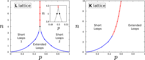
Figure 1: (colour online) Phase diagrams for the L and K lattices. Continuous transitions are indicated by blue dots and a single line and first order transitions by red dots and a double line. For the L lattice, the point $p=1/2,\,n=4$ lies in the extended phase, as shown in the inset.

Both lattices are defined on a graph $\cal G$ that has cubic symmetry; they differ in their link orientations. To construct the graph $\cal G$, take two interpenetrating cubic lattices $C_{1}\equiv{(2\mathbf{Z})}^{3}$ and $C_{2}\equiv(2{\mathbf{Z}}+1)^{3}$ as illustrated in Fig. 2. The edges (or links) of $\cal G$ are formed by the intersections of the faces of $C_{1}$ with the faces of $C_{2}$. The nodes of $\cal G$ lie on the midpoints of the edges of $C_{1}$ or of $C_{2}$ (although these edges do not themselves belong to $\cal G$), and the four links that meet at a node lie on two orthogonal axes.

Figure 2: (color online) Left: a cube of $C_{1}$, with the lines of intersection with $C_{2}$ marked in red. These lines form the links of the $L$ and $K$ lattices. Right: with the orientations corresponding to the $L$ lattice added. The nodes lie on two sublattices, marked in yellow and black.

The L-lattice, illustrated in Fig. 3, has the property that both incoming links at a node lie on the same axis, and both outgoing links lie on the other axis (Fig. 4). This is sufficient to fix the orientation of all links on the lattice up to a global two-fold choice, which is arbitrary. The K-lattice has the alternative property that all links lying on a given axis are directed in the same sense (Fig. 5). In addition, links on nearest neighbour parallel axes are oppositely directed.

To specify in a more formal way the assignment of weights $p$ and $1-p$ in each case, we describe the unique configuration of loops contributing to $Z_{\rm loops}$ at $p=0$. For both lattices this consists solely of non-planar loops of six links. Each such loop can be defined by giving the coordinates of an initial site and the orientations of the first three steps from this site, since the remaining three steps have opposite orientations in the same order. The unit cell of the three-dimensional L-lattice contains four such loops, and that of the K-lattice contains two loops, as set out in Table 1.

We take links to have unit length. In simulations we use cubic samples of linear size $L$ with periodic boundary conditions. The number of nodes is then $N=3L^{3}/4$ for both lattices.

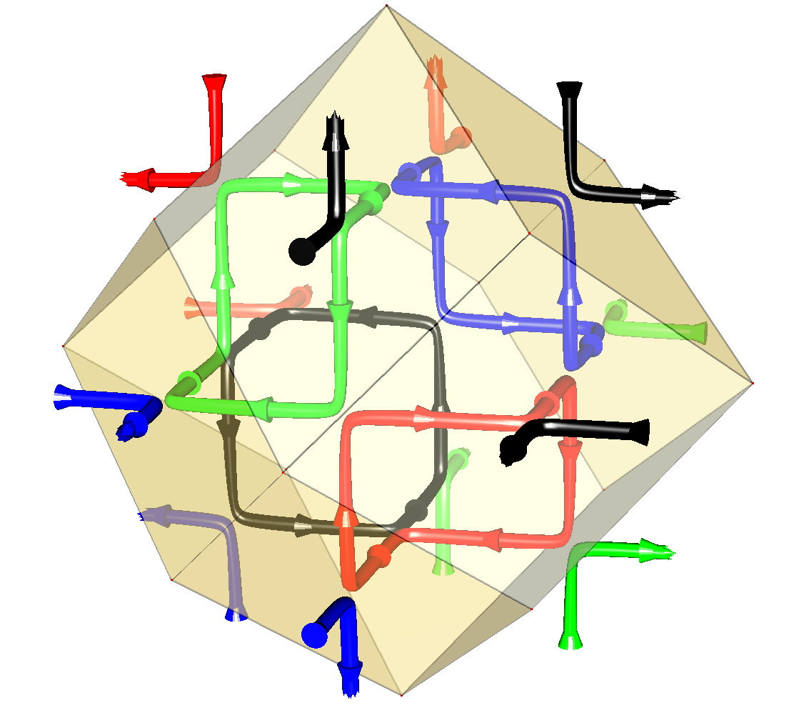
Figure 3: (color online) Loops on the 3D L lattice at $p=0$. The bounding planes of the Wigner Seitz unit cell are shaded and each of the four loops of Table 1 has a different colour.

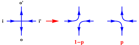
Figure 4: (color online) A node on the L lattice, together with the labelling of links used in Eq. (7).

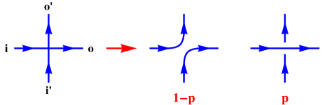
Figure 5: (color online) A node on the K lattice, together with the labelling of links used in Eq. (7).

L-Lattice
$(0,1,0)$	$\hat{\bf x}$	$\hat{\bf y}$	$\hat{\bf z}$
$(1,0,1)$	$\hat{\bf x}$	$\hat{\bf y}$	$-\hat{\bf z}$
$(0,1,2)$	$\hat{\bf x}$	$-\hat{\bf y}$	$-\hat{\bf z}$
$(1,2,1)$	$\hat{\bf x}$	$-\hat{\bf y}$	$\hat{\bf z}$

K-Lattice
$(0,0,0)$	$\hat{\bf x}$	$\hat{\bf y}$	$\hat{\bf z}$
$(1,0,0)$	$\hat{\bf x}$	$-\hat{\bf z}$	$-\hat{\bf y}$

Table 1: Initial position and first three steps of the hexagons forming the L- and K-lattices.

III Field theory description

In this section we give a simple way to connect the loop models to field theory (Sections III.1 and III.2). We also discuss (Sec. III.3) the relationship between loop observables and correlation functions of the field theory, and the use of a replica-like limit or supersymmetry (SUSY) to extend the range of correlation functions expressible in that field theory. A compact account of these ideas appeared in Ref. prl, ; see also the related discussion in Ref. vortex paper, . We discuss the relation to quantum problems described by the same field theories in Sec. III.4.

III.1 Introduction of local degrees of freedom

The loop models may be related to lattice ‘magnets’ for spins located on the links $l$ of the lattice. Neglecting for now complications associated with replicas or supersymmetry (and taking $n$ to be a positive integer), these spins are $n$-component complex vectors ${\bf z}_{l}$ with

$${\bf z}_{l} =(z^{1}_{l},\ldots,z^{n}_{l}) {\rm and}\qquad{\bf z}_{l}^{\dagger}{\bf z}_{l} =n.$$ (4)

The action for these degrees of freedom will be chosen so that a graphical expansion generates the sum over loop configurations defining $Z_{\text{loops}}$. This leads to a $U(1)$ gauge symmetry,

$${\bf z}_{l}\sim e^{i\phi_{l}}{\bf z}_{l},$$ (5)

implying that the spins live on $CP^{n-1}$ — the manifold of fixed-length complex vectors modulo the equivalence (5).

The required action may be written as a sum of contributions from nodes. Letting the trace ‘$\operatorname{Tr}$’ stand for an integral over the fixed-length vectors ${\bf z}$, normalised so $\operatorname{Tr}1=1$, we write

$$Z=\operatorname{Tr}\exp\bigg{(}-\sum_{\text{nodes}}S_{\text{node}}\bigg{)}.$$ (6)

To define $S_{\text{node}}$ label the links at a node as in Figs. 4 and 5, with the weight $p$ pairing being $i\rightarrow o$, $i^{\prime}\rightarrow o^{\prime}$ and the weight $1-p$ pairing being $i\rightarrow o^{\prime}$, $i^{\prime}\rightarrow o$. Then

$$\exp\left(-S_{\text{node}}\right)=p\,({\bf z}_{o}^{\dagger}{\bf z}_{i})({\bf z}_{o^{\prime}}^{\dagger}{\bf z}_{i^{\prime}})+(1-p)\,({\bf z}_{o}^{\dagger}{\bf z}_{i^{\prime}})({\bf z}_{o^{\prime}}^{\dagger}{\bf z}_{i}).$$ (7)

The total action is invariant under the gauge transformation (5), as the phase $\phi_{l}$ cancels between the terms for the two nodes adjacent to link $l$.

The two terms in $e^{-S_{\text{node}}}$ are in correspondence with the two node configurations in the loop model. This leads to a simple expression for the partition function in terms of loop configurations $\mathcal{C}$, of the form

$$\operatorname{Tr}\prod_{\text{nodes}}\exp\left(-S_{\text{node}}\right)=\sum_{\mathcal{C}}\,W_{\mathcal{C}}\prod_{\text{loops in }\mathcal{C}}\operatorname{Tr}\,({\bf z}_{1}^{\dagger}{\bf z}^{\phantom{{\dagger}}}_{2})\ldots({\bf z}_{\ell}^{\dagger}{\bf z}^{\phantom{{\dagger}}}_{1}).$$ (8)

Here we have used the labels $1,\ldots,\ell$ for the links lying on a loop of length $\ell$ and $W_{\mathcal{C}}=p^{N_{p}}(1-p)^{N_{1-p}}$ is the weight associated with the nodes. Next, perform the integrals over the ${\bf z}$s using $\operatorname{Tr}z_{l}^{\alpha}\bar{z}_{l}^{\beta}=\delta^{\alpha\beta}$ (repeated indices are summed throughout) to obtain

$$\operatorname{Tr}\,({\bf z}_{1}^{\dagger}{\bf z}^{\phantom{{\dagger}}}_{2})\ldots({\bf z}_{\ell}^{\dagger}{\bf z}^{\phantom{{\dagger}}}_{1}) =\operatorname{Tr}\,(\bar{z}_{1}^{\alpha_{1}}z_{2}^{\alpha_{1}})(\bar{z}_{2}^{\alpha_{2}}z_{3}^{\alpha_{2}})\ldots(\bar{z}_{\ell}^{\alpha_{\ell}}z_{1}^{\alpha_{\ell}})$$

$$=\delta^{\alpha_{1}\alpha_{2}}\delta^{\alpha_{2}\alpha_{3}}\ldots\delta^{\alpha_{\ell}\alpha_{1}}.$$ (9)

The Kronecker deltas force the spin indices $\alpha_{i}$ to be equal for all the links $i$ on a given loop. The remaining free index gives the desired sum over $n$ colours for each loop, so that

$$Z=\sum_{\mathcal{C}}\sum_{\begin{subarray}{c}\text{loop}\\ \text{colours}\end{subarray}}W_{\mathcal{C}}=Z_{\text{loops}}.$$ (10)

This establishes the correspondence between the loop models and models with local ‘magnetic’ degrees of freedom. Its utility is that we may now make the simplest conjectures for the models’ continuum descriptions, taking account of the $SU(n)$ global and $U(1)$ gauge symmetries of the lattice action appearing in Eq. (6).

Note that this lattice action is complex-valued. When coarse-graining is considered carefully, the naive real action resulting from a derivative expansion has to be supplemented with imaginary terms associated with hedgehog defects,interacting but for the transitions considered in this paper the consequence of these terms is only to renormalise the parameters in the effective Lagrangian, and not to change the naive result.

III.2 Continuum limit

Let us exchange the vector ${\bf z}$, which is a redundant parametrisation of $CP^{n-1}$, for the gauge-invariant matrix $Q$, defined by

$$Q^{\alpha\beta}=z^{\alpha}\bar{z}^{\beta}-\delta^{\alpha\beta}.$$ (11)

$Q$ is Hermitian and traceless, and obeys the nonlinear constraint $(Q+1)^{2}=n\,(Q+1)$.

In the continuum we may either retain this constraint, giving the $CP^{n-1}$ $\sigma$ model

$$\mathcal{L}_{\text{$\sigma$}} =\frac{1}{2g}\operatorname{tr}\,(\nabla Q)^{2} (\text{and constraint on $Q$}),$$ (12)

or we may use a formulation in which $Q$ is an arbitrary traceless Hermitian matrix, giving the soft spin model

$$\mathcal{L}_{\text{soft}}=\operatorname{tr}\left(\nabla Q\right)^{2}+t\operatorname{tr}Q^{2}+g\operatorname{tr}Q^{3}+\lambda\operatorname{tr}Q^{4}+\lambda^{\prime}(\operatorname{tr}Q^{2})^{2}.$$ (13)

The existence of hedgehog defects (possible because of the nontrivial second homotopy group $\pi_{2}(CP^{n-1})=\mathbb{Z}$) means that the second formulation is arguably more natural in three dimensions. Hedgehogs are known to play an important role in the vicinity of the critical point, and they proliferate in disordered phase; they are of course irrelevant in the ordered phase.Kamal Murthy ; Motrunich Vishwanath ; senthil et al dcp ; quantum criticality beyond ; Read Sachdev spin peierls ; Haldane O(3) sigma model In order to accommodate them in the sigma model, the constraint must be relaxed in the defect core, and the regularisation-dependent physics in the core then determines a finite fugacity for defects — the condensed formulation (12), with only the single parameter $g$, is therefore slightly misleading.

The manifold $CP^{1}$ is simply the sphere, so at the special value $n=2$ the above field theories reduce to the $\sigma$ model and soft spin incarnations of the $O(3)$ model. At this value of $n$, the cubic term in $\mathcal{L}_{\text{soft}}$ vanishes, and there is only one quartic term. The $O(3)$ spin $S$ is related to $Q$ via the Pauli matrices. Setting $Q=\frac{1}{\sqrt{2}}\sigma^{i}S^{i}$ in $\mathcal{L}_{\text{soft}}$ gives

$$\mathcal{L}_{\text{soft}}=(\nabla S)^{2}+t\,S^{2}+u\,(S^{2})^{2}$$ (14)

with $u=\lambda^{\prime}+\lambda/2$.

This description leads us to expect continuous transitions in the $O(3)$ universality class for the $n=2$ models. Continuous transitions are also expected for $n<2$. For $n>2$, the naive expectation is a first order transition, as a result of the cubic term in $\mathcal{L}_{\text{soft}}$. However, as we will see in Sec. IV, fluctuations can invalidate this mean field prediction when the spatial dimension is less than four, and so numerical work is required to determine what happens in 3D.

III.2.1 Aside: compact and non-compact $CP^{n-1}$ models

The field theories described above should be distinguished from the related ‘non-compact’ $CP^{n-1}$ models, in which ${\bf z}$ is coupled to a non-compact $U(1)$ gauge field $A$:

$$\mathcal{L}_{\text{NCCP}^{n-1}}=\frac{1}{2}|(\nabla-iA){\bf z}|^{2}+\kappa(\nabla\times A)^{2}+\mu|{\bf z}|^{2}+\lambda|{\bf z}|^{4}.$$

The universal behaviour of the ‘compact’ $CP^{n-1}$ models (those discussed in this paper) may also be captured by gauge theories similar to the above, but with a compact $U(1)$ gauge symmetry. This distinction is discussed in Refs. senthil et al dcp, , quantum criticality beyond, and Motrunich Vishwanath, . In the compact case, configurations of the gauge field $A$ are allowed that contain Dirac monopoles. This leads to confinement of ${\bf z}$ quanta, so that at long distances only the neutral degrees of freedom in $Q$ play a role, and we return to the field theories already discussed.

In our microscopic models, the gauge symmetry is compact: the parameter $\phi_{l}$ in (5) is defined only modulo $2\pi$. A subtlety is that in some cases senthil et al dcp ; quantum criticality beyond critical points in models with compact gauge symmetry may be described by emergent non-compact gauge theories in the continuum. This occurs as a result of the suppression of Dirac monopoles — or, as it turns out equivalently, of hedgehog configurations in $Q$.

III.3 Correlation functions

The graphical expansion of the lattice field theory (6) generates a sum over loop configurations in which each loop carries a colour index $\alpha=1,\ldots,n$. This leads straightforwardly to expressions for correlation functions of $Q$ in terms of the probabilities of geometrically-defined events. These relationships are those one would expect from viewing the loops as worldlines of ${\bf z}$ quanta, with one of the spatial directions taken as the imaginary time direction for a quantum problem. These worldlines come in $n$ colours, one for each component of ${\bf z}$, and since $z^{\alpha}$ is a complex field they carry an orientation distinguishing particles from antiparticles.

In particular, the operator $Q_{l}^{\mu\nu}=z_{l}^{\mu}\bar{z}_{l}^{\nu}$ with $\mu\neq\nu$ absorbs an incoming strand/worldline of colour $\mu$ and emits an outgoing one of colour $\nu$. More precisely, the effect of this operator on the graphical expansion is to force the loop passing through link $l$ to change colour from $\mu$ to $\nu$ there. This follows from the fact that the presence of the operator changes the single link integral appearing in Eq. 9 from $\operatorname{Tr}z_{l}^{\alpha}\bar{z}_{l}^{\alpha^{\prime}}=\delta^{\alpha\alpha^{\prime}}$ to $\operatorname{Tr}z_{l}^{\alpha}\bar{z}_{l}^{\alpha^{\prime}}Q_{l}^{\mu\nu}=A\,\delta^{\alpha\nu}\delta^{\alpha^{\prime}\mu}$ (for $\mu\neq\nu$), with $A=n/(n+1)$.

We can use $Q$ to represent the probability $G(l,l^{\prime})$ that two links lie on the same loop, since the correlator $\left\langle Q^{12}_{l}Q^{21}_{l^{\prime}}\right\rangle$ receives contributions only from configurations in which $l$ and $l^{\prime}$ are joined (by a loop with one arm of colour $1$ and one arm of colour $2$) and

$$G(l,l^{\prime})=\frac{n}{A^{2}}\big{\langle}Q^{12}_{l}Q^{21}_{l^{\prime}}\big{\rangle}.$$ (15)

In this expression the factor of $n$ compensates for the fact that there is no sum over colour indices for the loop passing through $l_{1}$ and $l_{2}$. In the terminology of loop models, $Q^{\alpha\beta}$ is a ‘two-leg’ operator.

For convenience, we here use the off-diagonal elements of $Q$ to write geometrical correlators, but all $Q$ correlators can be expressed in terms of loops; for example $\left\langle\operatorname{tr}Q_{l}Q_{l^{\prime}}\right\rangle=(n-1)A\,G(l,l^{\prime})$. We may think of the diagonal components, e.g. $Q^{11}_{l}$, as operators which measure the colour of a link.

The two-leg correlator $G(l,l^{\prime})$ generalises to $2k$-leg correlators $G_{2k}$, which give the probability that two regions are joined by $2k$ strands. For example, on the lattice we can define $G_{4}$ as the probability that four separate strands connect two nodes. In the continuum, such correlators may be written

$$G_{2k}(x,y)\propto\left\langle[Q^{12}(x)]^{k}[Q^{21}(y)]^{k}\right\rangle,$$ (16)

where $Q(x)$ is the continuum field.

So far, the correlators we have considered involve only two distinct spin indices $\alpha=1,2$. They can therefore be written down so long as the spin ${\bf z}$ has at least two components ($n\geq 2$). More complex correlation functions may require the use of more indices. For example, if $n\geq k$ we can express the probability that a single loop passes through all the links $l_{1},\ldots,l_{k}$, in that order as

$$G(l_{1},\ldots,l_{k})=\frac{n}{A^{k}}\left\langle Q^{12}_{l_{1}}Q^{23}_{l_{2}}\ldots Q^{k1}_{l_{k}}\right\rangle.$$ (17)

III.3.1 Replicas / SUSY

These formulas highlight a potential problem. The complexity of the geometrical correlation functions we can represent is limited by the number $n$ of spin components at our disposal, which in turn is set by the loop fugacity. The problem is most acute at $n=1$, when we cannot represent any correlation functions at all.

The simplest way to get around this is to calculate the desired correlation function assuming that $n$ is sufficiently large, and subsequently analytically continue to the required value of $n$. This is a standard idea in the study of geometrical problems such as loop models and percolation, and is analogous to the replica trick in disordered systems. For simplicity, we will use this replica-like limiting procedure in this paper. However it should be noted that there is also a more rigorous alternative, which is to augment the field theory with additional fermionic degrees of freedom in such a way that the resulting field theory has a global supersymmetry. For our purposes in this paper, replicas and SUSY are equivalent and it is easy to translate between them.

The supersymmetric construction is described in Refs. candu et al, ; read saleur, ; prl, and vortex paper, , and leads to the so-called $CP^{n+k-1|k}$ model, in which ${\bf z}$ is replaced by a supervector ${\bf\psi}$ with $n+k$ bosonic components $z^{\alpha}$ and $k$ fermionic ones $\chi^{\alpha}$, so that

$$\psi=(z^{1},\ldots,z^{n+k},\chi^{1},\ldots,\chi^{k}).$$ (18)

The supersymmetry ensures that the value of $k$ does not affect the partition function or its expansion in loop configurations. However, increasing $k$ yields more operators.

III.3.2 Phases of the $CP^{n-1}$ model

When the $CP^{n-1}$ spins are disordered, correlators such as $G(x,y)$ decay exponentially, indicating that long loops are exponentially suppressed. At a critical point, the anomalous dimension $\eta$ of the spin $Q$ determines the decay of $G(x,y)$,

$$G(x,y)\sim|x-y|^{-(1+\eta)},$$ (19)

the fractal dimension of a loop duplantier saleur percolation ; scaling relations

$$d_{f}=\frac{5-\eta}{2},$$ (20)

and the probability $P(l)$ that the loop passing though a given link is of length $l$:

$$P(l) \sim l^{1-\tau}, \tau =\frac{11-\eta}{5-\eta}.$$ (21)

If the mean field estimate $\eta=0$ is a good approximation, the loops have a fractal dimension close to $5/2$.

When the spins are ordered, $G(x,y)$ is long-ranged, indicating the appearance of extended loops. The nature of these extended loops in a large, finite sample of linear size $L$ depends on whether curves are allowed to terminate at the boundary or whether all loops are closed. In the former case the extended loops have length $O(L^{2})$, since the loops in this phase have fractal dimension two. In the latter case they have a length $O(L^{3})$: although the fractal dimension of a segment of radius $\lesssim L$ is still two, the number of times a given extended loop crosses the sample is of order $L$. We now focus on the case with only closed loops, which pertains to our simulations with periodic boundary conditions.

The magnitude of order parameter in this phase is proportional to the fraction of links lying on extended loops. To demonstrate this, consider applying a magnetic field $h\sim{\cal O}(L^{-2})$ that couples to $Q$ via a term in the action $\delta S=-h\sum_{l}Q^{11}_{l}$. In the spin language, the field fixes the direction of symmetry breaking to ${\bf z}\sim(1,0,\ldots,0)$ and the order parameter is simply the average $\langle Q^{11}_{l}\rangle$ calculated in the presence of the weak field $h$. In the graphical expansion, $\delta S$ endows loops of colour $\alpha=1$ with a small additional length fugacity: finite strands are insensitive to $h$ but extended strands are forced to be of colour $\alpha=1$, so that they alone contribute to $\langle Q^{11}_{l}\rangle$.

In the extended phase, contributions to the $2k$-leg correlation functions $G_{2k}$ may be split up according to how many of the strands are finite and how many are infinite, and the power law decay of the geometrical correlation function depends only on the former. Let $\widetilde{G}_{m}$ be the probability that $m$ finite strands connect $x$ and $y$, irrespective of the number of infinite strands. Then we find

$$\widetilde{G}_{m}(x,y)\sim|x-y|^{-m}.$$ (22)

These exponents are also independent of how many of the finite strands are oriented from $x$ to $y$ (rather than the reverse) and whether the strands join together form a single loop or many loops. The exponent values indicate that within the extended phase a single walk is Brownian on long scales, having for example a fractal dimension of two.

To arrive at this result, consider again the effect of a weak symmetry breaking field, with $\delta S=-h\sum_{l}Q^{11}_{l}$. We can then regard the operators $z^{\alpha}$ and $\bar{z}^{\alpha}$ for $\alpha>1$ as absorbing/emitting strands which must be finite, while $z^{1}$ and $\bar{z}^{1}$ absorb/emit strands that may be extended. At large separations, the dominant contribution to any correlator is given by setting $z^{1}$ equal to a constant (determined by the strength of long range order) while contributions from components with $\alpha>1$ are proportional to Goldstone mode correlators, with two-point functions that decay inversely with separation. For example the correlator $\left\langle(z^{1}\bar{z}^{2})^{m}(x)(\bar{z}^{1}z^{2})^{m}(y)\right\rangle$, which forces $m$ finite strands to propagate from $x$ to $y$, decays as $|x-y|^{-m}$. This argument is readily generalised to give Eq. (22).

III.4 Transfer matrices and quantum magnets

The link colours provide a convenient basis for the transfer matrix, which acts between ‘time’ slices formed by planes of the lattice and which defines an associated quantum Hamiltonian. We briefly review a standard simple example,afflecknew then describe the qualitative features of the Hamiltonians corresponding to the 3D loop models.

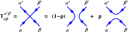
Figure 6: (color online) Graphical representation of the transfer matrix for a single node. The indices $\alpha,\beta,\alpha^{\prime},\beta^{\prime}$ denote link colours. Imaginary time increases in the vertical direction, with the lower links being at time $\tau$ and the upper links at time $\tau+\Delta\tau$.

Consider first of all the transfer matrix $T$ for a single node of the type shown in Fig. 6. In component form this is $T^{\alpha^{\prime}\beta^{\prime}}_{\alpha\beta}$, where the upper indices are the colours of the links at time $\tau+\Delta\tau$, and the lower indices those at time $\tau$. This matrix has two terms

$$T^{\alpha^{\prime}\beta^{\prime}}_{\alpha\beta}=(1-p)\delta^{\alpha^{\prime}}_{\alpha}\delta^{\beta^{\prime}}_{\beta}+p\,\delta^{\alpha^{\prime}\beta^{\prime}}\delta_{\alpha\beta}$$ (23)

corresponding to the two node configurations. The partition function $\operatorname{tr}T^{N}$ defines a quasi-one-dimensional loop model with $N$ nodes. The transfer matrix is also the imaginary time evolution operator for a two-site quantum problem with Hamiltonian $H$, related via

$$T=e^{-\Delta\tau H}.$$ (24)

Each site (we label them $A$ and $B$) has an $n$-dimensional Hilbert space, spanned by kets $\left|\alpha\right\rangle_{A}$ and $\left|\alpha\right\rangle_{B}$ respectively. In terms of these

$$T =(1-p)\mathbb{1}+p\sum_{\alpha\beta}\left|\alpha\right\rangle_{A}\left|\alpha\right\rangle_{B}\left\langle\beta\right|_{A}\left\langle\beta\right|_{B}$$ (25)

$$=(1-p)\mathbb{1}+p\,n\,\mathcal{P}_{AB}.$$ (26)

In the second line $\mathcal{P}_{AB}$ is the projector onto the state $\frac{1}{\sqrt{n}}\sum_{\alpha}\left|\alpha\right\rangle_{A}\left|\alpha\right\rangle_{B}$. This state is a singlet under $SU(n)$ transformations that act as

$$\left|\alpha\right\rangle_{A} \longrightarrow U_{\alpha\beta}\left|\beta\right\rangle_{A} {\rm and}\quad\left|\alpha\right\rangle_{B} \longrightarrow U^{*}_{\alpha\beta}\left|\beta\right\rangle_{B}.$$ (27)

The degrees of freedom at $A$ and $B$ are $SU(n)$ spins, transforming in the fundamental and antifundamental representation respectively.

At $n=2$ they are standard spin-1/2 degrees of freedom. In this case it is convenient to relabel the basis states as $S_{z}$ eigenstates for spin operators ${\bf S}_{A}$ and ${\bf S}_{B}$,

$$\left|1\right\rangle_{A} =\left|\uparrow\right\rangle_{A}, \left|{1}\right\rangle_{B} =\left|\downarrow\right\rangle_{B},$$

$$\left|2\right\rangle_{A} =\left|\downarrow\right\rangle_{A}, \left|{2}\right\rangle_{B} =-\left|\uparrow\right\rangle_{B}.$$ (28)

Both spins then transform in the same representation (this is possible at $n=2$ because the fundamental representation of $SU(2)$ is pseudoreal). The singlet takes the usual form $\frac{1}{\sqrt{2}}[\left|\uparrow\right\rangle_{A}\left|\downarrow\right\rangle_{B}-\left|\downarrow\right\rangle_{A}\left|\uparrow\right\rangle_{B}]$, and the projector onto it is $\mathcal{P}_{AB}=1/4-{\bf S}_{A}.{\bf S}_{B}$.

For the single node we can easily extract the form of the Hamiltonian. Dropping an additive constant, it is

$$H=J\,\mathcal{P}_{AB},$$ (29)

with $J=\Delta\tau^{-1}\ln[1+pn/(1-p)]$.

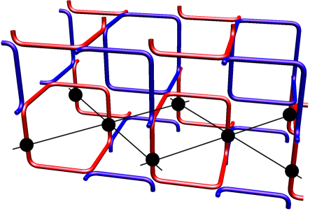
Figure 7: (color online) The K lattice at $p=0$: this short loop phase corresponds to a staggered dimer state. The square lattice for the associated quantum problem is formed by the links and filled circles in a time slice, shown in black.

For 2D or 3D loop models, the Hamiltonian will not generally take a simple explicit form. If we insist on one, we must take a continuum limit in imaginary time — this corresponds to making the node weights anisotropic in such a way that the transfer matrix becomes close to the identity. This procedure is standard for the loop model on the two-dimensional L lattice:afflecknew the resulting Hamiltonian describes a nearest-neighbour spin chain, and the node parameter in the loop model controls dimerisation in the strength of the exchange. For the 3D models we take the view that the precise form of $H$ is less important than the degrees of freedom, symmetries and phase structure of $H$.

For both the L and K lattice we take imaginary time to run parallel to the vertical axis of Fig. 2. The links intersecting a time slice (which is of thickness two link lengths in the K lattice and four in the L lattice) then form a square lattice with lattice spacing $\sqrt{2}$, as shown in Fig. 7. One sublattice consists of upgoing and the other of downgoing links; as in the single-node example, this leads to an $SU(n)$ magnet with spins in the fundamental representation on one sublattice and in the antifundamental representation on the other. The transfer matrix $T$ for a given lattice is a sum over configurations within the timeslice, in analogy to Eq. (23). The phase structure of the models is like that of nearest-neighbour $SU(n)$ magnets with dimerization in the strength of the exchange, $H=\sum_{\left\langle ij\right\rangle}J_{ij}\mathcal{P}_{ij}$; of course the actual Hamiltonian, given by the logarithm of $T$, would not take this simple form.

The extended phase in the loop models corresponds to the Néel phase, while the short-loop phase corresponds to a dimerised phase. The pattern of dimerisation in a short-loop phase can be seen from the representative configuration in which all loops have the minimal length of six. These loops connect the links within a timeslice in pairs; in the quantum problem singlets form between the paired sites. For the L lattice there are four packings of minimal-length loops, corresponding to the four columnar packings of singlets on the square lattice. When $p=1/2$ these packings are related by lattice symmetry, which is broken when $p\neq 1/2$. That is, varying $p$ away from $1/2$ imposes a specific dimerisation in the couplings in $H$. For the K lattice there is only a single packing of minimal-length loops, which corresponds to a staggered packing of singlets.

IV The $CP^{n-1}$ model near $n=2$ and $d=4$

At $n=2$, when the cubic term in $\mathcal{L}_{\text{soft}}$ vanishes, the upper critical dimension of the $CP^{n-1}$ model is four rather than six. This allows a double expansion in

$$\Delta=n-2\qquad\quad\text{and}\qquad\quad\epsilon=4-d.$$ (30)

This idea has been discussed previously for the $Q$-state Potts model, where the expansion is about the Ising limit.Newman Riedel Muto The conclusions below for the $CP^{n-1}$ model are qualitatively identical. In particular, a universal $n_{c}$ appears, which is greater than the mean field value two when $d<4$.

To begin with, recall the Wilson-Fisher Wilson Fisher renormalisation group (RG) equations for the $O(3)$ (or $CP^{1}$) model (14). To lowest nontrivial order these are, after rescaling $u\rightarrow u/22$,

$$\frac{\mathrm{d}u}{\mathrm{d}\ln L} =\epsilon u-u^{2}, \frac{\mathrm{d}t}{\mathrm{d}\ln L} =\left(2-\frac{5}{11}u\right)t.$$ (31)

Setting $t=0$, there are fixed points at $u=0$ and $u=\epsilon$. For $\epsilon>0$, the latter is stable in the $u$ direction, and describes the critical $CP^{1}$ model, while the former is unstable in the $u$ direction and describes the tricritical point.

We now consider a formal expansion of these equations in $\Delta$ (compare the approach to the $2+\epsilon$ dimensional $O(n)$ model in Ref. Cardy Hamber, ), deferring the field-theoretic interpretation until Sec. IV.0.1. The leading contribution is a modification to the RG equation for $u$:

$$\frac{\mathrm{d}u}{\mathrm{d}\ln L} =-a\Delta+\epsilon u-u^{2}.$$ (32)

The consistent scaling is to take $\Delta$ to be $O(\epsilon^{2})$, and $u$ to be $O(\epsilon)$ as at the Wilson Fisher fixed point. Here $a$ is an undetermined universal constant, assumed positive in order to give sensible RG flows.

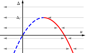
Figure 8: (color online) RG fixed points and flows in the $(u,\Delta)$ plane for $d<4$, showing critical (red full curve) and tricritical (blue dashed curve) fixed points merging at $\Delta_{c}$.

Fig. 8 shows the resulting RG fixed points in the $(u,\Delta)$ plane for fixed $\epsilon>0$. As $\Delta$ is increased from zero, the critical and tricritical fixed points approach each other, annihilating at a critical $n_{c}$ given to this order by

$$n_{c}\simeq 2+\frac{\epsilon^{2}}{4a}.$$ (33)

The thermal and leading irrelevant exponents at the critical point are

$$y_{t} \simeq 2-\frac{5}{22}\left(\epsilon+\sqrt{\epsilon^{2}-4a\Delta}\right), y_{\text{irr}} \simeq-\sqrt{\epsilon^{2}-4a\Delta}.$$

The anomalous dimension $\eta$ is $O(\epsilon^{2})$, as in the $O(N)$ model. Analogous formulas hold for the Potts model.Newman Riedel Muto

Precisely at $n_{c}$, the irrelevant exponent vanishes and there are logarithmic corrections to scaling. Above $n_{c}$, there are no fixed points: the RG flows go off to large negative $u$, which we interpret as a first order transition.

The size of discontinuities at this first order transition decrease rapidly as $n$ approaches $n_{c}$ from above. Integrating Eq. (32) from a microscopic scale at which $u$ is positive and of order one to the scale of the correlation length $\xi$, where $u$ is negative and of order one, gives

$$\xi\sim\exp\left(\frac{2\pi}{\epsilon}\sqrt{\frac{n_{c}-2}{n-n_{c}}}\right).$$ (34)

Similar forms hold for other quantities such as the latent heat.cardy nauenberg scalapino The asymptotic form $\xi\sim\exp\left(\text{const.}/\sqrt{n-n_{c}}\right)$ is in fact more general than the lowest-order expansion we consider here, since it depends only on the mechanism by which the critical point disappears at $n_{c}$.baxter latent heat ; cardy nauenberg scalapino ; Newman Riedel Muto

In Fig. 9 we show the RG fixed points in the $(d,u)$ plane for $n>2$ and $n<2$. Note that when $n<2$ the fixed points below four dimensions are smoothly connected to those above. This is in agreement with our belief that a $6-\epsilon$ expansion is possible in the model with $n=1$.vortex paper For $n>2$ a branch of fixed points appears above four dimensions. These fixed points, which are at negative $u$, are not expected to correspond to genuine critical points, as a result of unboundedness of the fixed point potential (this phenomenon is present even in the $O(N)$ model Wilson Fisher ).

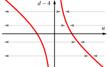
Figure 9: (color online) RG fixed points and flows in the $(u,d)$ plane. Left: for $n<2$. Right: for $n>2$.

IV.0.1 More concrete picture

Let us rewrite the soft spin $CP^{n-1}$ model as

$$\mathcal{L}_{\text{soft spin}}=\operatorname{tr}(\nabla Q)^{2}+t\operatorname{tr}Q^{2}+\frac{u}{22}\operatorname{tr}Q^{4}+V(Q)\,,$$ (35)

collecting the operators that vanish at $n=2$ into $V(Q)$. There is one of these at cubic and one at quartic order, and we allow for higher terms with

$$V(Q)=g_{1}\operatorname{tr}Q^{3}+g_{2}\left(\operatorname{tr}Q^{4}-\frac{1}{2}(\operatorname{tr}Q^{2})^{2}\right)+\ldots$$ (36)

The two operators shown explicitly vanish when $n=2$, by virtue of the tracelessness of $Q$.

The RG equations for $t$ and $u$ must of course be independent of the $g_{i}$ when $n=2$, so any term which depends on the latter must have a coefficient proportional to $\Delta$. This phenomenon also occurs in the Potts model.Newman Riedel Muto To the order that we require, the RG equations for $u$ and $g_{i}$ hence have the form

$$\frac{\mathrm{d}u}{\mathrm{d}\ln L} =\epsilon u-u^{2}-\Delta\,f(g_{1},g_{2},\ldots),$$

$$\frac{\mathrm{d}g_{i}}{\mathrm{d}\ln L} =\beta_{i}(g_{1},g_{2},\ldots),$$ (37)

and we have checked explicitly that the $f$ term is of order $\Delta$, not higher. The cubic coupling $g_{1}$ is strongly relevant at the four-dimensional Gaussian fixed point, which obstructs a perturbative calculation of $f$ and $\beta_{i}$. However to obtain Eq. (32) we need only assume that the $g_{i}$ flow to fixed point values $g_{i}^{*}$ under the RG equations (37), and expand around these with $g_{i}=g_{i}^{*}+\delta g_{i}$, obtaining

$$\frac{\mathrm{d}u}{\mathrm{d}\ln L} \simeq\epsilon u-u^{2}-\Delta f(g_{1}^{*},g_{2}^{*},\ldots), \frac{\mathrm{d}\delta g_{i}}{\mathrm{d}\ln L} \simeq-b_{ij}\delta g_{j}.$$

The first of these equations yields Eq. (32), with $a=f(g_{1}^{*},g_{2}^{*},\ldots)$. The second yields subleading (order one) irrelevant exponents associated with the operators in $V(Q)$.

IV.0.2 Two upper critical dimensions at $n=2$

In order to analytically continue in $n$ it is important to realise that it is the operators in $V(Q)$, and not their couplings, which vanish when $n=2$. We may consider higher-dimensional versions of the loop models discussed here, and this observation leads to the conclusion that for $n=2$ such models have two distinct upper critical dimensions.

For correlators that can be written down using only two spin indices, we do not need a replica limit or SUSY. We set $n=2$ directly, giving the $O(3)$ model with upper critical dimension four. At the critical point these correlators will thus have Gaussian behaviour for $d\geq 4$. However for correlators that require more than two indices, we are forced either to analytically continue in $n$ or to use SUSY. In either case, the cubic term reappears (in the SUSY formulation, the soft-spin $CP^{n+k-1|k}$ model, it is $\operatorname{str}Q^{3}$, where $\operatorname{str}$ is the supertrace), leading to a non-Gaussian theory below six dimensions. These correlators are thus expected to have nontrivial behaviour for $d<6$. This could be tested numerically by a simulation in four dimensions.

V Simulations

V.1 Monte Carlo procedure

To describe our Monte Carlo procedure, we explain in the following how configurations are labelled, how an initial state is constructed, and what Monte Carlo updates are used. Our approach is similar to ones used in loop algorithms for simulations of quantum spin systems.QMCreviews

We generate the fugacity $n$ from a sum on loop colours, and so a configuration of the model is specified by the pairing of incoming and outgoing links at each node and by a colour for each link, with the constraint that all links belonging to the same loop must have the same colour. This approach imposes the requirement that $n$ is integer: we have developed an alternative algorithm that works for any real positive $n$, but it is less efficient.

An initial state is constructed by choosing at random the configuration of each node with the specified probability. A colour is associated with each loop, chosen with equal probability from $n$ alternatives.

Subsequent states are generated using three kinds of Monte Carlo move. In the first, a node is chosen at random. If the two loop strands passing through the chosen node have different colours, the node configuration is not changed, but if they both have the same colour, it is changed according to the following rules. Denote the node configuration that has probability $1-p$ by $\alpha$ and the one with probability $p$ by $\beta$. For $p<1/2$ a node in configuration $\alpha$, is changed to $\beta$ with probability $p/(1-p)$, and one in configuration $\beta$ is always changed to $\alpha$. For $p>1/2$, a node in configuration $\alpha$ is always changed to $\beta$, and a node in configuration $\beta$ is changed to $\alpha$ with probability $(1-p)/p$. In the second type of Monte Carlo move, a link is chosen at random and the colour of all the links of the loop to which it belongs is changed to a different colour, chosen with uniform probability from the $n-1$ possibilities. The third type of move is to re-colour all loops in the system, with the new colours selected independently and at random for each loop. It is designed to ensure that the colours of short loops equilibrate efficiently.

The first two types of move are intercalated, with ten node updates followed by one colour change. For a sample with $N$ nodes we call $N/10$ such sequences a Monte Carlo sweep. Measurements are performed every two Monte Carlo sweeps and the third type of move is applied after each measurement sweep. The autocorrelation function of the energy is used to estimate a correlation time.

We consider loop models with an integer number of colours $1\leq n\leq 10$, and system sizes of up to $7.5\times 10^{5}$ links for $n\geq 2$, and $6\times 10^{9}$ for $n=1$. The minimum number of Monte Carlo sweeps used is $10^{5}$ for any $n$, $p$ and $L$, and increases with decreasing $L$.

V.2 Observables

We measure observables for the loop models that are related to those of the $CP^{n-1}$ model. In particular, we calculate quantities with the same scaling behaviour as the stiffness, susceptibility, order parameter and heat capacity of the sigma model, and we compute the Binder cumulant for the energy. We also evaluate the fractal dimension of loops. Detailed definitions and expected finite-size scaling behaviour are as follows.

V.2.1 Stiffness

As a quantity equivalent to the sigma model stiffness, we study the average number $n_{\rm w}(p,L)$ of curves winding around the sample in a given direction.stiffness More precisely, we pick a plane of the lattice and count for each configuration the number of sections of trajectory that leave this plane on a given side and wind around the sample to reach the same plane from the opposite side. It is a property of the models that for each such trajectory section winding in the given direction, there is another trajectory section winding in the opposite direction. For large sample size $n_{\rm w}(p,L)$ approaches zero in a phase with only short loops, and is proportional to $L$ in a phase with extended trajectories. If there is a continuous transition between these phases at a critical point $p_{\rm c}$ with correlation length exponent $\nu$, one expects the finite-size scaling behaviour

$$n_{\rm w}(p,L)=f_{\rm w}(L^{1/\nu}[p-p_{\rm c}])\;.$$ (38)

V.2.2 Susceptibility

The susceptibility of the sigma model can be expressed in the standard way as the spatial integral of the connected part of a two-point correlation function. With this as motivation, let $n(s)$ be the number of loops of length $s$ in a given configuration. Then the spatial integral of the two-point correlation function in Eq. (15) is proportional to $\langle{\sum}_{s}s^{2}n(s)\rangle$, where $\langle\ldots\rangle$ denotes an average over configurations. We split $n(s)$ into contributions $n_{\text{ext}}(s)$ and $n_{\text{loc}}(s)$ from extended and localised loops, with $n(s)=n_{\text{loc}}(s)+n_{\text{ext}}(s)$. Here we define extended loops to be those that contribute to $n_{\mathrm{w}}$. We then take as our definition of the susceptibility $\chi$

$$\chi L^{3} = \left\langle\sum_{s=0}^{L^{3}}s^{2}n(s)\right\rangle-\left\langle\sum_{s=0}^{L^{3}}s^{2}n_{\rm ext}(s)\right\rangle$$ (39)

$$= \left\langle\sum_{s=0}^{L^{3}}s^{2}n_{\rm loc}(s)\right\rangle\,.$$

On approaching a continuous transition, $\chi$ in an infinite system diverges with a critical exponent $\gamma$, while the expected scaling form in a finite system is

$$\chi=L^{\gamma/\nu}f_{\chi}(L^{1/\nu}[p-p_{c}])\;.$$ (40)

V.2.3 Order parameter

The value of the order parameter $\cal M$ can be extracted from the correlation function used to compute the susceptibility: the disconnected part – the second term on the right hand side of Eq. (39) – is proportional to ${\cal M}^{2}$. Hence we take

$${\cal M}L^{3}=\sqrt{\left\langle\sum_{s=0}^{L^{3}}s^{2}n_{\rm ext}(s)\right\rangle}\;.$$ (41)

At a continuous transition $\cal M$ varies with critical exponent $\beta$ and has the finite-size scaling behaviour

$${\cal M}=L^{-\beta/\nu}f_{\cal M}(L^{1/\nu}[p-p_{c}])\;.$$ (42)

V.2.4 Heat capacity

The heat capacity $C$ can be expressed in the usual way in terms of fluctuations in the energy. Absorbing a constant, we take from Eq. (3)

$$CL^{3}=\langle N_{p}^{2}\rangle-\langle N_{p}\rangle^{2}\,.$$ (43)

Introducing the critical exponent $\alpha$, we expect the finite-size scaling form

$$C=L^{-\alpha/\nu}f_{C}(L^{1/\nu}(p-p_{c}))\;.$$ (44)

V.2.5 Fractal dimension

To evaluate the fractal dimension $d_{f}$ of loops we measure the end-to-end distance $R(s)$ of portions of trajectories as a function of arc-length $s$. Evidently, while on average $R(s)$ increases with $s$ for small $s$, it must decrease to zero for each loop as $s$ approaches the loop length. To eliminate these finite-loop effects we retain only those contributions to $R(s)$ for which $s$ is less than one-third of the loop length. We then expect

$$\langle R(s)\rangle\propto s^{1/d_{f}}\,.$$ (45)

V.2.6 Binder cumulant

As a tool for distinguishing between first order and continuous transitions, we compute the Binder cumulant $V_{L}$ for the energy. This is defined by

$$V_{L}\equiv 1-\frac{1}{3}\frac{\left\langle n_{p}^{4}\right\rangle}{\left\langle n_{p}^{2}\right\rangle^{2}}\;.$$ (46)

V.3 Critical behaviour for $CP^{1}$

We use the loop model with $n=2$ as a test case, since there is a clear expectation that it should have a phase transition with critical behaviour in the same universality class as that of the $O(3)$ model in three dimensions, which in turn is known to high precision from previous simulations.O(3) numerics We study system sizes $32\leq L\leq 100$. We find similar results on both the K-lattice and the L-lattice. For conciseness we present data only in the former case.

The existence of a phase transition is evident from the behaviour of $n_{\rm w}(p,L)$ displayed in Fig. 10. The winding number is expected to decrease with increasing system size in a phase with only short loops, and to increase with system size in a phase with extended loops. In confirmation, curves of $n_{\rm w}(p,L)$ as a function of $p$ cross at a common point for different $L$. To illustrate this in detail, we show in the lower right inset to Fig. 10 the crossing point $p^{*}$ for curves at two successive system sizes $L_{1}$ and $L_{2}$ as a function of the inverse of the geometrical mean size $L=\sqrt{L_{1}L_{2}}$. We fit this to the form $p_{\rm c}+a/L^{b}$ (full line), obtaining $p_{\rm c}=0.38138(4)$ and $b=3.0(5)$. For a first approach to determining the exponent $\nu$, we plot in the upper left inset to Fig. 10 the gradient $dn_{\rm w}(p^{*})/dp$ as a function of $L$ on a double logarithmic scale. As expected from Eq. (38), the data fit well to a straight line. The inverse gradient of this line yields the estimate $\nu=0.68(3)$.

An alternative method for the determination of $\nu$ is to attempt a scaling collapse of all data. In this approach we construct the scaling function numerically, allowing for a non-linear dependence of the scaling variable on distance from the critical point and including corrections to scaling governed by a leading irrelevant exponent $y_{\rm irr}<0$. The quality of the fit and the number of fitting parameters supported by the data are judged by the value of $\chi^{2}$ compared to the number of degrees of freedom. We use for the scaling variable

$$x=L^{1/\nu}\left[(p-p_{\rm c})+A(p-p_{\rm c})^{2}\right]\,,$$ (47)

finding that inclusion of the term in $(p-p_{\rm c})^{2}$ is justified by the fit, while addition of a further term proportional to $(p-p_{\rm c})^{3}$ would not be. We construct a fitting function $f_{\rm splines}(x)$ using cubic B-splines with 16 points. We combine it with corrections to scaling, characterised by $y_{\rm irr}$ and an $m$th order polynomial $P_{m}(x)$, in two alternative ways: either as

$$f_{1}(x,L)=f_{\rm splines}(x)[1+P_{m}(x)L^{y_{\rm irr}}]$$ (48)

or as

$$f_{2}(x,L)=f_{\rm splines}(x)+P_{m}(x)L^{y_{\rm irr}}\,.$$ (49)

We achieve the best fit using the form $f_{1}(x,L)$ with $m=1$. It yields $\nu=0.706(8)$, $y_{\rm irr}=-1.0(3)$ and $p_{\rm c}=0.38141(5)$ with $\chi^{2}=300.5$ for 291 degrees of freedom. This scaling collapse is illustrated in Fig. 4 of Ref. prl, .

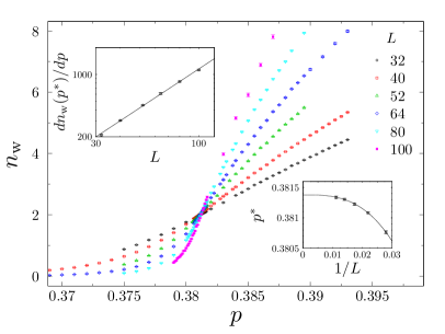
Figure 10: (color online) Winding number for $n=2$. Main panel: $n_{\rm w}(p,L)$ as a function of $p$ for different system sizes $L$. Left inset: ${\rm d}n_{\rm w}(p)/{\rm d}p$ at crossing points $p^{*}$ vs. $L$ on log-log scales. Right inset: $p^{*}$ vs $1/L$.

As a further demonstration that our results for $n=2$ are indeed compatible with the universality class of the $O(3)$ model, we attempt a scaling collapse using the best available exponent estimateO(3) numerics for that class, $\nu=0.7112$. We omit finite size corrections, leaving the value of $p_{\rm c}$ as the only fitting parameter. The fitted value of $p_{\rm c}$ is $0.38120(10)$. This procedure results in good overlap of data from different systems sizes, as illustrated in Fig. 11.

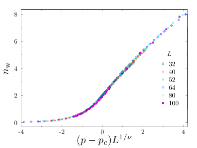
Figure 11: (color online) Scaling collapse at $n=2$ of $n_{\rm w}(p)$ as a function of $L^{1/\nu}(p-p_{\rm c})$ using the best estimate of $\nu$ for the $O(3)$ model, without allowing for corrections to scaling.

We analyse data for the susceptibility and for the order parameter by adapting the approach summarised for the winding number in Eqns. (47) - (49). Taking into account the fits for all three observables, our best exponent estimates are $\nu=0.708(5)$ and $\gamma=1.39(1)$.

As an alternative, we also attempt collapse of data for the susceptibility using the best exponent estimates for the $O(3)$ model. The outcome is shown in Fig. 12: we plot $\chi L^{-\gamma/\nu}/(1+AL^{y_{\rm irr}})$ as a function of $L^{1/\nu}(p-p_{\rm c})$, fixing the values O(3) numerics $\nu=0.7112$, $\gamma=1.3960$ and $y_{\rm irr}=-0.8$. This leaves the values of $p_{\rm c}$ and $A$ as the only fitting parameters: the fitted values are $p_{\rm c}=0.38145(15)$ and $A=1.58(20)$. Again we obtain good overlap of data from different system sizes. We note that the values of $p_{\rm c}$ obtained using different methods are consistent within statistical errors.

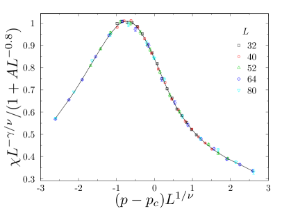
Figure 12: (color online) Scaling collapse of data for susceptibility $\chi$ as a function of $(p-p_{\rm c})L^{1/\nu}$ at $n=2$ using for the exponents the best estimates for the $O(3)$ model.

Measurement of the fractal dimension of loops at the critical point yields $d_{\rm f}=2.475(20)$, implying $\eta=0.05(4)$, which is consistent with the result $\eta=0.0375(5)$ from previous high-precision Monte Carlo studies.O(3) numerics

We have repeated the same procedure for data from the L-lattice with similar results. From an analysis of the winding number, the susceptibility and the order parameter on this lattice, we obtain for the critical exponents the values $\nu=0.708(4)$ and $\gamma=1.383(10)$. These values again agree within errors with the best estimates for the $O(3)$ model.O(3) numerics

V.4 Identifying the order of transitions

The phase transition in the loop model on the K-lattice may be continuous or first order, depending on the value of $n$, and in this subsection we set out our approaches to determining the order of the transition from Monte Carlo data. Indeed, as discussed in Sec. IV, while we expect a continuous transition at $n=2$ from the equivalence to the $O(3)$ model, a first order transition would be natural for larger $n$ since Landau theory admits a cubic invariant if $n\not=2$. Our results for the K-lattice are in fact consistent with a continuous transition at $n=3$ and with first order transitions for $n\geq 4$. Note that the loop model on the L-lattice at $n\geq 5$ has no extended phase but exhibits a first-order transition at $p=1/2$ between two symmetry-related short-loop phases (see Fig. 1).

Distinguishing the order of a transition using simulations is delicate in marginal cases because of finite size effects. We therefore begin by discussing simple limiting examples. For $n=2$ we take it as established by the results of Sec. V.3 that the transitions on both lattices are continuous. On the other hand, the transition for $n=4$ on the K lattice is first order. To demonstrate this, we show in Fig. 13 the distribution of $n_{+}=N_{p}/(N_{p}+N_{1-p})$ (essentially the energy distribution) for three different values of $p$ very close to the transition. The double-peaked form, characteristic of a first-order transition, is very clear.

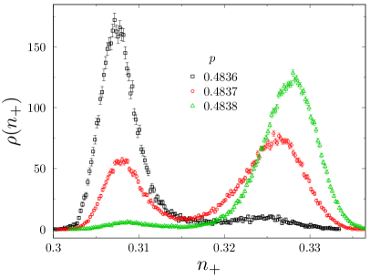
Figure 13: (color online) Evidence for a first order transition at $n=4$ on the K-lattice for $L=80$: probability distribution of the energy showing the double-peaked form that is characteristic of a first-order transition.

More generally, an established diagnostic for the order of a transition is provided by the Binder cumulant $V_{L}$. In a system with a continuous transition one expects $\lim_{L\to\infty}V_{L}=2/3$ everywhere in the phase diagram, critical points included, but at a first order transition point $\lim_{L\to\infty}V_{L}<2/3$.binder

We illustrate behaviour of the Binder cumulant for $n=3$ on the K-lattice (anticipated to be a marginal case) in Fig. 14. As a function of $p$, $V_{L}$ has a minimum near the transition point and approaches $V_{L}=2/3$ far from the transition on either side. The minimum becomes shallower with increasing $L$ and the key issue is its limiting value. To focus on this we show in Fig. 15 the difference $2/3-[V_{L}]_{\rm min}$ as a function of $L$ on a double logarithmic scale. The data for $n=4$ on the K-lattice indicate a finite limiting value for $2/3-[V_{L}]_{\rm min}$ at large $L$, and hence a first order transition in this case. For other cases ($n=2$ and $n=3$ on both lattices, and $n=4$ on the L-lattice) the data fits a straight line with finite slope, as expected for a continuous transition. If any of these transitions is in fact first order, the correlation length at the transition must be larger than 100 lattice spacings (but see Sec. V.6 for a discussion of the L lattice transition with $n=4$).

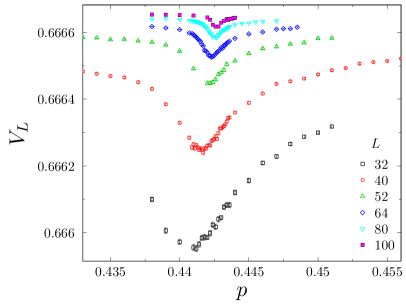
Figure 14: (color online) Binder cumulant $V_{L}$ at $n=3$: behaviour of $V_{L}$ as a function of $p$ for a sequence of system sizes $L$.

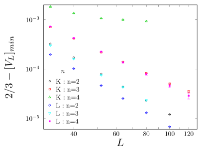
Figure 15: (color online) Distinguishing continuous from first order transitions: log-log plot of the dependence on system size of the deviation $2/3-[V_{L}]_{\rm min}$ of the minimum value of the Binder cumulant $V_{L}$ from its theoretical value far from the transition. Data give evidence of a continuous transition at $n=2$ and $n=3$, and a first order transition on the K-lattice at $n=4$.

A measure of the discontinuity at a first order transition is given by $\Delta V(n)=\lim_{L\to\infty}2/3-[V_{L}]_{\rm min}$. For the loop model with $n\geq 4$ on the K-lattice we can obtain $\Delta V(n)$ with high precision. As shown in Fig. 16, the dependence of $\Delta V(n)$ on $n$ can be fitted to functional forms with a critical value $n_{\rm c}$ separating first order from continuous transitions that is larger than or close to 3. Thus the transition at $n=3$ is apparently second order, but $n_{c}<4$.

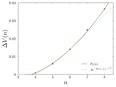
Figure 16: The discontinuity $\Delta V(n)$ at first order transitions as a function of $n$, with fits to a second-order polynomial $P_{2}(n)$ and to the functional form $Ae^{-B(n-n_{c})^{-1/2}}$ motivated by Eq. (34). The fitted values below which the transition is continuous are $n_{\rm c}=3.78(4)$ and $n_{\rm c}=3.0(2)$, respectively.

An alternative method for characterising the nature of a transition is to construct a parameter-free scaling function that has a fixed limiting form if the transition is continuous, but not if it is first order. Consider for loop models the probability $P_{1}(p,L)$ that a configuration has exactly one winding curve, as a function of the average number $\langle n_{\rm W}(p,L)\rangle$ of winding curves. At a continuous transition one expects this function to be independent of system size, provided finite-size corrections to scaling are not important. By contrast, the number of spanning curves jumps at a first order transition, from zero in one phase to a value proportional to $L$ in the other phase. In this case $P_{1}(p,L)$ therefore approaches zero with increasing $L$ for all $\langle n_{\rm W}(p,L)\rangle$. In Fig. 17 we present this scaling function for $n=2$ (top inset), $n=3$ (main panel) and $n=4$ (bottom inset) for the K-lattice. The data for different system sizes lie on a single curve for $n=2$, while those for $n=4$ do not. Data for $n=3$ lie close to a single curve, although with larger deviations than at $n=2$. Provided these deviations may be attributed to finite-size corrections to scaling, the results of this analysis are consistent with the ones from the behaviour of the Binder cumulant.

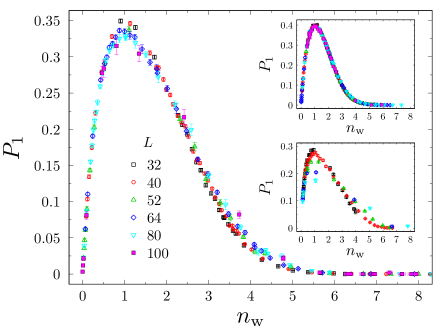
Figure 17: (color online) Parameter-free scaling collapse: data for the probability $P_{1}(p,L)$ that a configuration has exactly one winding curve as a function of the average number $n_{\rm W}(p,L)$ of winding curves: main panel $n=3$; top inset $n=2$. Bottom inset: contrasting behaviour at $n=4$.

V.5 Critical behaviour for $CP^{2}$

Having established that the transition in the loop model with $n=3$ on the K-lattice has a correlation length that appears divergent and certainly grows larger than the largest accessible system sizes, we next characterise the critical behaviour. We follow the methods described in Sec. V.3 for $n=2$, except that in the present case independent values of critical exponents are not available.

The unscaled data for $n_{\rm w}(p,L)$ are displayed as a function of $p$ for several system sizes in Fig. 18 (main panel): the transition point is apparent from the crossing of curves for different system sizes. In the lower right inset to Fig. 18 we show the dependence of the probability $p^{*}$ at which data for two successive sizes cross, as a function of the inverse of the geometrical mean $L$ of these sizes. The continuous curve is a fit of the form $p_{\rm c}+a/L^{b}$, with $p_{\rm c}=0.44291(2)$ and $b=2.1(3)$. In the upper left inset to Fig. 18 we plot the dependence on $L$ of the winding number $n_{\rm w}$ at which data for two successive sizes cross. It shows that the finite size effects in this observable are not negligible. Nevertheless, we have undertaken a scaling collapse of all the data, using a non-linear scaling variable and including corrections to scaling as in Sec. V C. Results were presented previously in Fig. 4 of Ref. prl, . Improved statistics of data obtained more recently makes $\chi^{2}$ values for the collapse larger and seems to indicate that the finite size effects are not fully under control. The best estimates that we obtain are $\nu=0.51(2)$, where the quoted error is statistical and systematic errors are difficult to estimate.

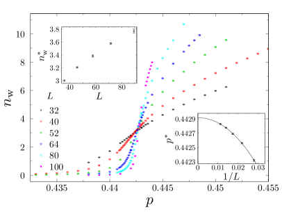
Figure 18: (color online) Scaling for $n=3$. Main panel: number of winding curves $n_{\rm w}(p)$ plotted as a function of $p$ for different system sizes $L$. Left inset: dependence of $n_{\rm w}$ at crossing points on $L$. Right inset: $p^{*}$ vs $1/L$.

By contrast, we find that analysis of the scaling behaviour of the susceptibility $\chi$ is more straightforward. Its dependence on $p$ and system size is shown in Fig. 19. It has a peak near the critical point which grows with $L$. Plotting $\chi L^{-\gamma/\nu}$ as a function of $x=L^{1/\nu}[(p-p_{\rm c})+A(p-p_{\rm c})^{2}]$, these data exhibit scaling collapse, as illustrated in the inset to Fig. 19, with $\chi^{2}=53$ for 60 degrees of freedom. The exponent values resulting from this procedure are $\nu=0.542(16)$ and $\gamma/\nu=1.78(2)$, and $\gamma=0.97(2)$.

Figure 19: (color online) The susceptibility $\chi$ at $n=3$ for the K-lattice. Inset: scaling collapse of data in the main panel, using the scaling variable $x$ defined in Eq. (47)

Data for the heat capacity $C$ are presented in Fig. 20. It is strongly divergent at the transition but values in the smaller system sizes are dominated by a smooth background. To effect a scaling collapse we therefore subtract an $L$-independent contribution $C_{\rm reg}$ that varies smoothly with $p$, plotting $(C-C_{\rm reg})L^{-\alpha/\nu}$ as a function of $L^{1/\nu}[(p-p_{\rm c})+A(p-p_{\rm c})^{2}]$: see Fig. 20 inset. From this approach we obtain $\chi^{2}=73$ with 95 degrees of freedom; assuming the $d$-dimensional hyperscaling relation $\alpha=2-d\nu$, we find $\nu=0.526(15)$.

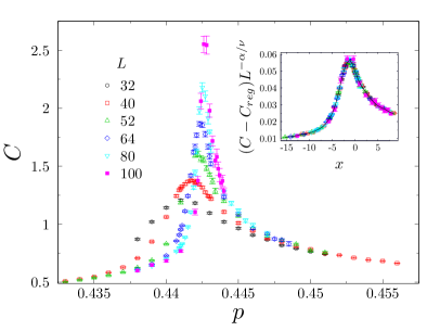
Figure 20: (color online) Heat capacity as a function of $p$ at $n=3$ for the K lattice. Inset: scaling collapse of the divergent contribution to the heat capacity.

Inclusion of corrections to scaling in the analysis of $\chi$ and $C$ does not change significantly our exponent estimates or the scaling collapse, and we were unable to determine a reliable value for $y_{\rm irr}$.

From a study of loops at the critical point (data not shown) we find the fractal dimension value $d_{f}=2.40(3)$. This implies $\eta=0.20(6)$, which is broadly consistent with the value $\eta=0.22(2)$ obtained using hyperscaling and our analysis of $\chi$.

Combining the results from our analysis of data on the K-lattice for $\chi$, $C$, the order parameter (not shown), and using bootstrap methods to determine errors, our best estimates for the two independent critical exponents are $\nu=0.536(13)$ and $\eta=0.23(2)$. The scaling relations $\gamma=(2-\eta)\nu$ and $\beta=\nu(1+\eta)/2$ imply $\gamma=0.97(2)$ and $\beta=0.33(1)$. The given uncertainties are obtained from a purely statistical analysis. The results may also be affected by systematic errors: from the dispersion in the values of $\nu$ obtained from analysis of different observables, we believe that the systematic errors in our exponent values are comparable in magnitude to the statistical ones.

Similar but less exhaustive analysis for the L-lattice gives compatible exponent values, although with much larger uncertainties.

V.6 L-lattice at $n=4$

The case $n=4$ on the L-lattice deserves specific discussion. In the phase diagram for this lattice (see Fig. 1) the line $p=1/2$ is within an extended phase for small $n$ and is the location of first-order transitions for large $n$. The point $p=1/2,\,n=n^{*}$ at which behaviour changes is expected to be a deconfined critical point.interacting At $n=4$ as a function of $p$ we find two distinct transitions, at $p_{c}$ and $1-p_{c}$, with $p_{\rm c}=0.4994(3)$, indicating that $n^{*}>4$. This is confirmed by the fact that behaviour at $p=1/2,\,n=4$ matches that expected in the extended phase: $n_{W}(1/2,L)$ is quite accurately proportional to $L$ for our largest system sizes. While we expect from universality and our results on the K lattice that the transition on the L lattice at $n=4$ should be first order, the proximity of the two transitions at $p_{c}$ and $1-p_{c}$ and of the critical point at $n^{*}$ makes in natural that the correlation length at the transition should be very large.

VI Concluding remarks

In summary, we have shown that the loop models we consider provide lattice representations of $CP^{n-1}$ $\sigma$ models, and we have set out the correspondence between loop observables and $\sigma$ model correlators. The models have phase transitions between paramagnetic and ordered phases, which we argue using an RG treatment are continuous for $n\leq n_{c}$; from simulations we give evidence that $n_{c}>3$ in three dimensions.

There is scope for further work on these and related loop models, in several directions. First, within the ordered phases of the models studied, a quantity of interest is the length distribution of long loops, expected to take a universal form.forthcoming length distribution paper Second, starting with the loop models on the L lattice at the symmetric point $p=1/2$, one can induce a phase transition by introducing an extra coupling. The short loop phase established in this way exhibits spontaneous symmetry breaking and the transition is a candidate for a deconfined critical point.interacting Third, and separately, models with undirected loops are interesting as representations of $RP^{n-1}$ $\sigma$ models, corresponding at $n=2$ to the $O(2)$ model and at $n=3$ to models for the liquid crystal isotropic-nematic transition: it would be of interest to investigate the order of the transition and possible critical behaviour as a function of $n$ for these undirected models.

- (1) A. Nahum, J. T. Chalker, P. Serna, M. Ortuño and A. M. Somoza, Phys. Rev. Lett. 107, 110601 (2011).
- (2) R. M. Bradley, J-M. Debierre, and P. N. Strenski, Phys. Rev. Lett 68 2332 (1992); R. M. Bradley, P. N. Strenski, and J-M. Debierre, Phys. Rev. A 45, 8513 (1992).
- (3) T. Vachaspati and A. Vilenkin, Phys. Rev. D 30, 2036 (1984).
- (4) K. O’Holleran, M. R. Dennis, F. Flossmann, and M. J. Padgett, Phys. Rev. Lett. 100, 053902 (2008).
- (5) I. A. Gruzberg, A. W. W. Ludwig, and N. Read, Phys. Rev. Lett. 82, 4524 (1999).
- (6) E. J. Beamond, J. Cardy, and J. T. Chalker, Phys. Rev. B 65, 214301 (2002).
- (7) N. Read and H. Saleur, Nucl.Phys. B 613, 409 (2001).
- (8) C. Candu, J. L. Jacobsen, N. Read, and H. Saleur, J. Phys. A 43, 142001 (2010).
- (9) M. Ortuño, A. M. Somoza, and J. T. Chalker, Phys. Rev. Lett. 102, 070603 (2009).
- (10) A. Nahum and J. T. Chalker, Phys. Rev. E 85, 031141 (2012).
- (11) For reviews, see: H. G. Evertz, Adv. Phys. 52, 1 (2003); A. W. Sandvik, AIP Conf. Proc. 1297, 135 (2010); R. K. Kaul, R. G. Melko, and A. W. Sandvik, arXiv:1204.5405.
- (12) K. Harada, N. Kawashima, and M. Troyer, Phys. Rev, Lett. 90, 117203 (2003).
- (13) K. S. D. Beach, F. Alet, M. Mambrini, and S. Capponi, Phys. Rev. B 80, 184401 (2009).
- (14) A. Nahum, J. T. Chalker, P. Serna, M. Ortuño and A. M. Somoza, in preparation.
- (15) B. B. Beard, M. Pepe, S. Riederer, and U.-J. Wiese, Phys. Rev. Lett. 94, 010603 (2005).
- (16) U. Wolff, Nucl. Phys. B 832, 520 (2010).
- (17) L. D. C. Jaubert, M. Haque and R. Moessner, Phys. Rev. Lett. 107, 177202 (2011); L. D. C. Jaubert, S. Piatecki, M. Haque, and R. Moessner, Phys. Rev. B 85, 054425 (2012).
- (18) V. Khemani, R. Moessner, S. A. Parameswaran, and S. L. Sondhi, Phys. Rev. B 86, 054411 (2012).
- (19) O. Schramm, Israel J. Math. 147, 221 (2005).
- (20) S. Grosskinsky, A. A. Lovisolo, and D. Ueltschi, J. Statist. Phys. 146, 1105-1121 (2012).
- (21) M. Campostrini, M. Hasenbusch, A. Pelissetto, P. Rossi, and E. Vicari, Phys. Rev. B 65, 144520 (2002).
- (22) R. K. Kaul, Phys. Rev. B 85, 180411 (2012).
- (23) S. Duane and M. B. Green, Phys. Lett. 103B, 359 (1981).
- (24) K. Kataoka, S. Hattori, and I. Ichinose, Phys. Rev. B 83, 174449 (2011).
- (25) H. Kunz and G. Zumbach, J. Phys. A 22, L1043 (1989).
- (26) J. Cardy, in 50 Years of Anderson Localization, ed. E. Abrahams (World Scientific, 2010).
- (27) F. D. M. Haldane, Phys. Rev. Lett. 61 1029 (1988).
- (28) N. Read and S. Sachdev, Phys. Rev. Lett. 62 1694 (1989).
- (29) T. Senthil, A. Vishwanath, L. Balents, S. Sachdev, and M. P. A. Fisher, Science 303, 1490 (2004).
- (30) T. Senthil, L. Balents, S. Sachdev, A. Vishwanath, and M. P. A. Fisher, Phys. Rev. B 70 144407 (2004).
- (31) M. Kamal and G. Murthy, Phys. Rev. Lett. 71 1911 (1993).
- (32) O. I. Motrunich and A. Vishwanath, Phys. Rev. B 70 075104 (2004).
- (33) H. Saleur and B. Duplantier, Phys. Rev. Lett. 58, 2325 (1987).
- (34) J. Kondev and C. L. Henley, Phys. Rev. Lett. 74, 4580 (1995).
- (35) I. Affleck, J. Phys.: Condens. Matter 2, 405 (1990).
- (36) K. E. Newman, E. K. Riedel, and S. Muto, Phys. Rev. B. 29 302 (1984).
- (37) K. G. Wilson and M. E. Fisher, Phys. Rev. Lett. 28, 240 (1972).
- (38) J. L. Cardy and H. W. Hamber, Phys. Rev. Lett. 45, 499 (1980).
- (39) J. L. Cardy, M. Nauenberg, and D. J. Scalapino, Phys. Rev. B 22, 2560 (1980).
- (40) R. J. Baxter, J. Phys. C 6, L445 (1973).
- (41) A. Nahum, P. Serna, A. M. Somoza and M. Ortuño, Phys. Rev. B 87, 184204 (2013).
- (42) See, for example, the derivation given in Sec. IVB of Ref. 2D unoriented,
- (43) M. S. S. Challa, D. P. Landau, and K. Binder, Phys. Rev. B 34, 1841 (1986).
- (44) A. Nahum, J. T. Chalker, P. Serna, M. Ortuño and A. M. Somoza, Phys. Rev. Lett. 111, 100601 (2013).