Electromagnetic two-point functions and the Casimir effect
in Friedmann-Robertson-Walker cosmologies

Abstract

We evaluate the two-point functions of the electromagnetic field in $(D+1)$-dimensional spatially flat Friedmann-Robertson-Walker universes with a power-law scale factor, assuming that the field is prepared in the Bunch-Davies vacuum state. The range of powers are specified in which the two-point functions are infrared convergent and the Bunch-Davies vacuum for the electromagnetic field is a physically realizable state. The two-point functions are applied for the investigation of the vacuum expectation values of the field squared and the energy-momentum tensor, induced by a single and two parallel conducting plates. Unlike to the case of conducting plates in the Minkowski bulk, in the problem under consideration the stresses along the directions parallel to the plates are not equal to the energy density. We show that, in addition to the diagonal components, the vacuum energy-momentum tensor has a nonzero off-diagonal component which describes energy flux along the direction normal to the plates. For a single plate this flux is directed from the plate. The Casimir forces are investigated in the geometry of two plates. At separations between the plates smaller than the curvature radius of the background spacetime, to the leading order, we recover the corresponding result in the Minkowski spacetime and in this case the forces are attractive. At larger separations, the influence of the curvature on the Casimir forces is essential with different asymptotic behavior for decelerated and accelerated expansions. In particular, for the latter case there is a range of powers of the expansion law in which the forces become repulsive at large separations between the plates.

PACS numbers: 04.62.+v, 04.20.Gz, 04.50.-h, 11.10.Kk

1 Introduction

Observational data on the large-scale structure of the Universe and on the cosmic microwave background indicate that at large scales the Universe is homogeneous and isotropic and its geometry is well described by the Friedmann-Robertson-Walker (FRW) metric. Because of the high symmetry, numerous physical problems are exactly solvable on this background and a better understanding of physical effects in FRW models could serve as a handle to deal with more complicated geometries. In particular, the investigation of quantum effects at the early stages of the cosmological expansion has been a subject of study in many research papers (see [1] for early investigations and [2]-[13] and references therein for later developments). Physical effects such as the polarization of the vacuum and particle creation by strong gravitational fields can have a profound impact on the dynamics of the expansion. They provide a natural mechanism for the damping of anisotropies in the early Universe and for a solution of the cosmological singularity problem. During an inflationary epoch, quantum fluctuations introduce inhomogeneities which explain the origin of the primordial density perturbations needed to explain the formation of the large-scale structure in the Universe [14].

The nontrivial properties of the vacuum are among the most interesting predictions of the quantum field theory. They are sensitive to both the local and global characteristics of the background spacetime in the early Universe. In particular, the properties of the vacuum state can be changed by the imposition of boundary conditions on the field operator. These conditions may be induced either by the presence of physical boundaries, like material boundaries in QED, or by the nontrivial topology of the background space. The both types of boundary conditions give rise to the modification of the spectrum for the vacuum fluctuations of a quantum field and, as a result, to the change in the vacuum expectation values (VEVs) of various physical observables. This effect for the electromagnetic field was first predicted by Casimir in 1948 and recently it has been experimentally confirmed with great precision (for reviews of the Casimir effect see Ref. [15]).

The explicit dependence of the VEVs on the bulk and boundary geometries can be found for highly symmetric backgrounds only. In particular, motivated by Randall-Sundrum-type braneworld models, investigations of the Casimir effect in anti-de Sitter spacetime have attracted a great deal of attention. In these models, the presence of the branes imposes boundary conditions on bulk quantum fields and, as a consequence of this, the Casimir-type forces arise acting on the branes. This provides a natural mechanism for the stabilization of the interbrane distance (radion), as required for a solution of the hierarchy problem. In addition, the Casimir energy contributes to both the brane and bulk cosmological constants and it has to be taken into account in any self-consistent formulation of the braneworld dynamics. The Casimir energy and forces in the geometry  of two parallel branes in anti-de Sitter bulk have been investigated in Refs. [16] by using either dimensional or zeta function regularization methods. Local Casimir densities for scalar and fermionic fields were studied in Ref. [17]. Higher-dimensional braneworld models in anti-de Sitter spacetime with compact internal spaces are considered in Ref. [18]. Another maximally symmetric gravitational background which plays an important role in cosmology is de Sitter spacetime. For a massive scalar field with general curvature coupling parameter, the Casimir densities in this background, induced by flat and spherical boundaries with Robin boundary conditions, have been investigated in Ref. [19] (for special cases of conformally and minimally coupled massless fields see Ref. [20]). More recently, the electromagnetic vacuum densities induced by a conducting plate in de Sitter spacetime have been discussed in Ref. [21]. In both cases of anti-de Sitter and de Sitter bulks, the curvature of the background spacetime decisively influences the properties of the vacuum at distances from the boundaries larger than the curvature scale of the background spacetime. Similar features were observed in the topological Casimir effect for scalar and fermionic fields, induced by toroidal compactification of spatial dimensions in de Sitter spacetime [22].

In the present paper we consider an exactly solvable problem for combined effects of the gravitational field and boundaries on the properties of the electromagnetic vacuum in a more general cosmological background. The two-point functions, the expectation values of the field squared and the energy-momentum tensor in the Bunch-Davies vacuum state are evaluated for the geometry of two parallel conducting plates in spatially flat FRW universes where the scale factor is a power of the comoving time (for the vacuum polarization and the particle creation in FRW cosmological models with power law scale factors see Refs. [5, 23, 24]). The vacuum expectation values of the energy-momentum tensor and the Casimir forces for conformally invariant scalar and electromagnetic fields in the geometry of curved boundaries on the background of FRW spacetime with negative spatial curvature have been recently investigated in Ref. [25]. In these papers, the boundaries are conformal images of flat boundaries in Rindler spacetime and the conformal relation between the FRW and Rindler spacetimes was used. Taking into account the recent interest to higher-dimensional models of both Kaluza-Klein and braneworld types and prospective applications in multidimensional cosmology, in the present paper we consider the case of arbitrary number of spatial dimensions $D$. The electromagnetic field is conformally invariant in $D=3$ and in this case the Casimir densities and forces for the Bunch-Davies vacuum state are simply obtained from the corresponding results in the Minkowski bulk by conformal transformation. In other dimensions this is not the case and the curvature of background spacetime leads to new qualitative features in the behavior of the vacuum characteristics. In particular, as it will be shown below, a nonzero energy flux appears along the direction normal to the plates.

The structure the paper is the following. In the next section we describe the background geometry and present a complete set of mode functions for the vector potential of the electromagnetic field. Then, these mode functions are used for the evaluation of the two-point functions for the vector potential and field tensor. In section 3, the mode functions and the two-point functions are derived in the region between two conducting plates. Section 4 is devoted to the investigation of the VEVs for the field squared and the energy-momentum tensor in the geometry of a single plate. The asymptotic behavior of the VEVs at small and large distances from the plate is discussed in detail. The VEVs in the geometry of two plates and the Casimir interaction forces are investigated in section 5. The main results of the paper are summarized in section 6.

2 Electromagnetic modes and two-point functions in boundary-free FRW spacetime

2.1 Background geometry

As background geometry we consider a spatially flat $(D+1)$-dimensional FRW spacetime with a power law scale factor versus time:

$$ds^{2}=dt^{2}-a^{2}(t)(d\mathbf{z})^{2},\;a(t)=a_{1}t^{c},$$ (1)

where $\mathbf{z}=(z^{1},\ldots,z^{D})$ are comoving spatial coordinates and $0<t<\infty$. For the scalar curvature corresponding to the line element (1) one has $R=Dc\left[(D+1)c-2\right]/t^{2}$. Below, in addition to the comoving time coordinate $t$, it is convenient to introduce the conformal time defined as $\tau=\int dt/a(t)$. In terms of the conformal time, for $c\neq 1$, one has

$$a(\tau)=a_{0}\eta^{b},\;t=\left[a_{1}(1-c)\tau\right]^{1/(1-c)},$$ (2)

where we have introduced the notations

$$\eta=|\tau|,\;b=c/(1-c),\;a_{0}=a_{1}(a_{1}|1-c|)^{b}.$$ (3)

Note that for $0<c<1$ one has $0<\tau<\infty$, and for $c>1$ one has $-\infty<\tau<0$. With this time coordinate, the line element is written in a conformally flat form: $ds^{2}=a^{2}(\tau)[d\tau^{2}-(d\mathbf{z})^{2}]$. Taking $c=0$ and $a_{1}=1$, from the formulas given below we obtain the corresponding results in the Minkowski bulk. In another limiting case, corresponding to $c\rightarrow\infty$, one has $b=-1$ and the scale factor (2) reduces to the one for de Sitter spacetime: $a(\tau)=a_{0}/\eta$ (in comoving time $a(t)=e^{t/a_{0}}$). In the case $c=1$ for the conformal time we have $\tau=a_{1}^{-1}\ln(t/t_{0})$ with the scale factor $a(\tau)=a_{1}t_{0}e^{a_{1}\tau}$, $-\infty<\tau<+\infty$. In the discussion below we shall assume that $c\neq 1$.

The energy density $\rho$ and the pressure $p$ corresponding to the line element (1) are found from the Einstein equations:

$$\rho=(D-1)\frac{Dc^{2}}{16\pi Gt^{2}},\;p=\left(D-1\right)\frac{c(2-cD)}{16\pi Gt^{2}},$$ (4)

with $G$ being the $(D+1)$-dimensional gravitational constant. Note that the energy density is always nonnegative, whereas the pressure can be either positive or negative. The equation of state for the source (4) is of barotropic type, $p=w\rho$, with the equation of state parameter $w=2/(cD)-1$. In the special case $c=2/(D+1)$ the Ricci scalar vanishes and this corresponds to a source of the radiation type. For $c=2/D$ the pressure is zero and one has another important special case of dust-matter driven models. In the case $c>1$, the expansion described by the scale factor (1) is accelerating. This type of expansion is employed in power law [26] and extended [27] inflationary models. The corresponding dynamics may be driven by a scalar field $\varphi$ with an exponential potential $V(\varphi)\propto e^{-\beta\varphi}$. In this case the parameter $c$ is given by the expression $c=4\beta^{-2}/(D-1)$ (see, for instance, [28]). Power law solutions with $c=2(n-1)(2n-1)/(D-2n)$ arise in higher-order gravity theories with the Lagrangian $R^{n}$ [29] . The results given below can also be applied to cosmological models driven by phantom energy for which $w<-1$. For the corresponding scale factor one has $a(t)=a_{1}(-t)^{c}$, $-\infty<t<0$, with $c<0$ and with the relation $t=-\left[a_{1}(c-1)\tau\right]^{1/(1-c)}$, $-\infty<\tau<0$. Note that we have a decelerating expansion for $0<c<1$ and an accelerating expansion for $c<0$ or $c>1$.

2.2 Mode functions

We consider the electromagnetic field with the action integral

$$S=-\frac{1}{16\pi}\int d^{D+1}x\,\sqrt{|g|}F_{\mu\nu}(x)F^{\mu\nu}(x),$$ (5)

in background described by the line element (1). In Eq. (5), $F_{\mu\nu}=\partial_{\mu}A_{\nu}-\partial_{\nu}A_{\mu}$ is the electromagnetic field tensor and $g$ is the determinant of the metric tensor. For the vector potential $A_{\mu}$ the gauge conditions $A_{0}=0$,$\;\nabla_{\mu}A^{\mu}=0$ will be imposed. The background geometry is spatially flat and we expand the vector potential in Fourier integral

$$A_{l}(x)=\int d\mathbf{k}\,A_{l}(\tau,\mathbf{k})e^{i\mathbf{k}\cdot\mathbf{z}},\;A_{l}(\tau,-\mathbf{k})=A_{l}^{\ast}(\tau,\mathbf{k}),$$ (6)

with shorthand notations $x=(\tau,\mathbf{z})$, $\mathbf{k}=(k_{1},\ldots,k_{D})$ and $\mathbf{k}\cdot\mathbf{z}=\sum_{l=1}^{D}k_{l}z^{l}$. From the gauge condition one has the relation $\sum_{l=1}^{D}k_{l}A_{l}(\tau,\mathbf{k})=0$.

Substituting the expansion (6) into the action integral and integrating over the spatial coordinates, one gets

$$S=\frac{(2\pi)^{D-1}}{4}\sum_{l=1}^{D}\int d\mathbf{k}\,\int d\tau\,a^{D-3}(\tau)\left[|\partial_{\tau}A_{l}(\tau,\mathbf{k})|^{2}-k^{2}|A_{l}(\tau,\mathbf{k})|^{2}\right],$$ (7)

with $k=|\mathbf{k}|$. This action gives rise to the following equation for the Fourier modes of the vector potential:

$$\partial_{\tau}\left[a^{D-3}(\tau)\partial_{\tau}A_{l}(\tau,\mathbf{k})\right]+a^{D-3}(\tau)k^{2}A_{l}(\tau,\mathbf{k})=0.$$ (8)

For the scale factor given by Eq. (2), the general solution of Eq. (8) is a linear combination of $\eta^{\nu}H_{\nu}^{(1)}(k\tau)$ and $\eta^{\nu}H_{\nu}^{(2)}(k\tau)$, where $H_{\nu}^{(1,2)}(x)$ are the Hankel functions and

$$\nu=\frac{1}{2}\left[1+\frac{(D-3)c}{c-1}\right].$$ (9)

One of the coefficients in the linear combination is determined from the normalization condition for the mode functions and the second coefficient is fixed by the choice of the vacuum state. In what follows we shall assume that the electromagnetic field is prepared in the Bunch-Davies vacuum state [23] for which $A_{l}(\tau,\mathbf{k})\sim\eta^{\nu}H_{\nu}^{(2)}(k\tau)$. With this choice, the two-point functions admit the Hadamard form. In the limit of slow expansion the Bunch-Davies vacuum is reduced to the standard Minkowskian vacuum. In the discussion below, we shall write the mode functions in terms of the Macdonald function by using the relation $H_{\nu}^{(2)}(k\tau)=(2i/\pi)e^{\nu\pi i/2}K_{\nu}(k\eta e^{s_{\tau}\pi i/2})$, where $s_{\tau}=\mathrm{sgn}(\tau)$. Note that $s_{\tau}=1$ for $0<c\,<1$ and $s_{\tau}=-1$ for other cases.

Hence, in the quantization procedure of the electromagnetic field as a complete set of mode functions we can take

$$A_{(\sigma\mathbf{k})l}(x)=C_{0}\epsilon_{(\sigma)l}\eta^{\nu}K_{\nu}(k\eta e^{s_{\tau}\pi i/2})e^{i\mathbf{k}\cdot\mathbf{z}},\text{ }l=1,\ldots,D,$$ (10)

with the polarization vectors $\epsilon_{(\sigma)l}$, $\sigma=1,\ldots,D-1$. For these vectors one has the relations

$$\sum_{l=1}^{D}\epsilon_{(\sigma)l}k_{l}=0,\;\sum_{l=1}^{D}\epsilon_{(\sigma)l}\epsilon_{(\sigma^{\prime})l}=\delta_{\sigma\sigma^{\prime}},$$ (11)

and

$$\sum_{\sigma=1}^{D-1}\epsilon_{(\sigma)l}\epsilon_{(\sigma)m}=\delta_{lm}-k_{l}k_{m}/k^{2}.$$ (12)

The coefficient $C_{0}$ in Eq. (10) is determined from the normalization condition:

$$\ \int d\mathbf{z}\,\sum_{l=1}^{D}[A_{(\sigma\mathbf{k})l}^{\ast}(x)\partial_{\tau}\ A_{(\sigma^{\prime}\mathbf{k}^{\prime})l}(x)-A_{(\sigma^{\prime}\mathbf{k}^{\prime})_{l}}(x)\partial_{\tau}\ A_{(\sigma\mathbf{k})l}^{\ast}(x)]=\frac{4\pi\delta_{\sigma\sigma^{\prime}}}{ia^{D-3}}\delta(\mathbf{k}-\mathbf{k}^{\prime}).$$ (13)

By making use of the relation

$$K_{\nu}(k\eta e^{-s_{\tau}\pi i/2})=e^{s_{\tau}\nu\pi i}K_{\nu}(k\eta e^{s_{\tau}\pi i/2})+s_{\tau}\pi iI_{\nu}(k\eta e^{s_{\tau}\pi i/2}),$$ (14)

with $I_{\nu}(x)$ being the modified Bessel function, the time-dependent part in the normalization integral is reduced to the Wronskian $W\{K_{\nu}(k\eta e^{s_{\tau}\pi i/2}),I_{\nu}(k\eta e^{s_{\tau}\pi i/2})\}$. In this way, for the normalization factor one gets

$$\left|C_{0}\right|^{2}=\frac{4a_{0}^{3-D}}{\left(2\pi\right)^{D}}.$$ (15)

For the Minkowski bulk we have $c=0$ and, hence, $\nu=1/2$. In this case the Macdonald function in Eq. (10) is reduced to the exponential one and we obtain the mode functions in the Minkowski spacetime. The special value $\nu=1/2$ is obtained for general $c$ in spatial dimensions $D=3$ and, again, the mode functions (10) reduce to the Minkowskian modes. This property is a consequence of the conformal invariance of the electromagnetic field in $D=3$.

2.3 Two-point functions

We consider a free field theory and all the properties of the vacuum state are encoded in the two-point functions. Two-point functions for vector fields in maximally symmetric spaces have been investigated in Ref. [30]. Though the background geometry under consideration is less symmetric, as it will be seen below, closed analytical expressions are obtained in this case as well. Expanding the field operator in terms of the complete set of mode functions and using the commutation relations for the annihilation and creation operators, we get the following mode sum formula for the two-point function of the vector potential:

$$\langle A_{l}(x)A_{m}(x^{\prime})\rangle_{0}=\sum_{\sigma=1}^{D-1}\int d\mathbf{k}\,A_{(\sigma\mathbf{k})l}(x)A_{(\sigma\mathbf{k})m}^{\ast}(x^{\prime}),$$ (16)

where and in what follows the Latin indices for tensors run over $1,2,\ldots,D$, and $\langle\cdots\rangle_{0}$ corresponds to the expectation value in the boundary-free FRW spacetime. Substituting the expression (10) for the mode functions and introducing the notation $\Delta\mathbf{z=z}-\mathbf{z}^{\prime}$, the following integral representation is obtained:

$$\langle A_{l}(x)A_{m}(x^{\prime})\rangle_{0}=\frac{4(\eta\eta^{\prime})^{\nu}}{(2\pi)^{D}a_{0}^{D-3}}\int d\mathbf{k}\,e^{i\mathbf{k}\cdot\Delta\mathbf{z}}\left(\delta_{lm}-\frac{k_{l}k_{m}}{k^{2}}\right)K_{\nu}(k\eta e^{s_{\tau}\pi i/2})K_{\nu}(k\eta^{\prime}e^{-s_{\tau}\pi i/2}).$$ (17)

In the integral with the term $\delta_{lm}$, we first integrate over the angular part of $\mathbf{k}$. The remaining integral over $k$ is convergent at the lower limit, $k=0$, under the condition $|\nu|<D/2$. From this condition, for the allowed values of the parameter $c$ one finds:

$$\left\{c<\frac{D+1}{2(D-1)}\right\}\cup\left\{c>\frac{D-1}{2}\right\}.$$ (18)

In this range of powers, the integral over $k$ is evaluated by using the formula from Ref. [31] and it is expressed in terms of the associated Legendre function of the first kind. We write the final result in terms of the hypergeometric function:

$$\int d\mathbf{k\,}e^{i\mathbf{k}\cdot\Delta\mathbf{z}}K_{\nu}(k\eta e^{s_{\tau}\pi i/2})K_{\nu}(k\eta^{\prime}e^{-s_{\tau}\pi i/2}) = \frac{\pi^{(D+1)/2}}{2\left(\eta\eta^{\prime}\right)^{D/2}}\frac{\Gamma(D/2+\nu)\Gamma(D/2-\nu)}{\Gamma\left((D+1)/2\right)}$$ (19)

$$\times F\left(\frac{D}{2}+\nu,\frac{D}{2}-\nu;\frac{D+1}{2};z\right),$$

where

$$z=1+\frac{\left(\Delta\eta\right)^{2}-|\Delta\mathbf{z}|^{2}}{4\eta\eta^{\prime}},$$ (20)

and $\Delta\eta=\eta-\eta^{\prime}$. With this integral, the two-point function is presented as

$$\langle A_{l}(x)A_{m}(x^{\prime})\rangle_{0} = \delta_{lm}\frac{(\eta\eta^{\prime})^{\nu-D/2}}{(4\pi)^{(D-1)/2}}\frac{\Gamma(D/2+\nu)\Gamma(D/2-\nu)}{\Gamma\left((D+1)/2\right)a_{0}^{D-3}}F\left(\frac{D}{2}+\nu,\frac{D}{2}-\nu;\frac{D+1}{2};z\right)$$ (21)

$$-\frac{4(\eta\eta^{\prime})^{\nu}}{(2\pi)^{D}a_{0}^{D-3}}\int d\mathbf{k}\,e^{i\mathbf{k}\cdot\Delta\mathbf{z}}\frac{k_{l}k_{m}}{k^{2}}K_{\nu}(k\eta e^{s_{\tau}\pi i/2})K_{\nu}(k\eta^{\prime}e^{-s_{\tau}\pi i/2}).$$

For the integral term in this formula one has no closed analytic expression. However, this part of the two-point function will not contribute to the two-point function for the field tensor and it will not be needed in the evaluation of the VEVs for the field squared and the energy-momentum tensor.

Given the two-point function for the vector potential, the corresponding function for the electromagnetic field tensor is evaluated as

$$\langle F_{\mu\lambda}(x)F_{\gamma\delta}(x^{\prime})\rangle_{0}=4\delta_{[\lambda}^{\rho}\partial_{\mu]}\delta_{[\delta}^{\sigma}\partial_{\gamma]}^{\prime}\langle A_{\rho}(x)A_{\sigma}(x^{\prime})\rangle_{0},$$ (22)

where the square brackets mean the antisymmetrization over the enclosed indices: $a_{\cdots[i_{j}\cdots i_{k}]\cdots}=(a_{\cdots i_{j}\cdots i_{k}\cdots}-a_{\cdots i_{k}\cdots i_{j}\cdots})/2$. The second term in the right-hand side of Eq. (21) does not contribute and one gets the following expressions:

$$\langle F_{0l}(x)F_{0m}(x^{\prime})\rangle_{0} = \frac{(\eta\eta^{\prime})^{\nu-D/2-1}}{2B_{D}a_{0}^{D-3}}\left[\left(\delta_{lp}\delta_{mq}-\delta_{lm}\delta_{pq}\right)\frac{\Delta z^{p}\Delta z^{q}}{2\eta\eta^{\prime}}\partial_{z}+\left(D-1\right)\delta_{lm}\right]F_{\nu-1}(z),$$

$$\langle F_{0m}(x)F_{pl}(x^{\prime})\rangle_{0} = -s_{\tau}\frac{(\eta\eta^{\prime})^{\nu-D/2-1}}{B_{D}a_{0}^{D-3}}\delta_{[pm}\delta_{l]q}\frac{\Delta z^{q}}{\eta}\left[\nu-\frac{D}{2}-1+\left(\frac{\eta+\eta^{\prime}}{2\eta^{\prime}}-z\right)\partial_{z}\right]F_{\nu}(z),$$ (23)

$$\langle F_{pl}(x)F_{qm}(x^{\prime})\rangle_{0} = \frac{(\eta\eta^{\prime})^{\nu-D/2-1}}{B_{D}a_{0}^{D-3}}\left(\delta_{[pr}\delta_{l][q}\delta_{m]s}\frac{\Delta z^{r}\Delta z^{s}}{\eta\eta^{\prime}}\partial_{z}+2\delta_{[pq}\delta_{l]m}\right)F_{\nu}(z),$$

with the notation

$$B_{D}=(4\pi)^{(D-1)/2}\Gamma\left((D+1)/2\right).$$ (24)

For the further convenience, in Eq. (23) we have introduced the function

$$F_{\nu}(z)=\frac{2}{D+1}\Gamma\left(\frac{D}{2}+1+\nu\right)\Gamma\left(\frac{D}{2}+1-\nu\right)F\left(\frac{D}{2}+1+\nu,\frac{D}{2}+1-\nu;\frac{D+3}{2};z\right).$$ (25)

The expression for the component $\langle F_{pl}(x)F_{0m}(x^{\prime})\rangle_{0}$ is obtained from that for $\langle F_{0m}(x)F_{pl}(x^{\prime})\rangle_{0}$ by changing the sign and by the interchange $\eta\rightleftarrows\eta^{\prime}$. The two-point function for the field tensor is obtained from the two-point function of the vector potential taking derivatives with respect to the coordinates. This enlarges the region for the values of the parameter $c$ for which the infrared divergences are absent in the integral representation of the correlator $\langle F_{\mu\lambda}(x)F_{\gamma\delta}(x^{\prime})\rangle_{0}$. Now, the infrared divergences for the Bunch-Davies vacuum state are absent under the condition $-D/2<\nu<D/2+1$ or, in terms of the parameter $c$,

$$\left\{c<\frac{D+1}{2(D-1)}\right\}\cup\left\{c>\frac{D+1}{4}\right\}.$$ (26)

For the values of $c$ outside this range the two-point function for the field tensor contains infrared divergences and the Bunch-Davies vacuum in a boundary-free FRW background is not a physically realizable state. Note that, in the limit $c\rightarrow\infty$ one has $\nu=D/2-1$ and from Eq. (22) we obtain the corresponding two-point functions in de Sitter spacetime with the scale factor $a(t)=e^{t/a_{0}}$ (see Ref. [21]).

Note that $F_{\nu}(z)$ is an even function of $\nu$: $F_{-\nu}(z)=F_{\nu}(z)$. An equivalent form for this function is obtained by using the linear transformation formula for the hypergeometric function [32]:

$$F_{\nu}(z)=\frac{2\Gamma\left(D/2+1-\nu\right)\Gamma\left(D/2+1+\nu\right)}{\left(D+1\right)(1-z)^{(D+1)/2}}F\left(\frac{1}{2}-\nu,\frac{1}{2}+\nu;\frac{D+3}{2};z\right).$$ (27)

Now, by taking into account that $F\left(0,1;c;z\right)=1$, for $\nu=1/2$ we get

$$F_{1/2}(z)=\frac{\Gamma^{2}\left((D+1)/2\right)}{(1-z)^{(D+1)/2}}.$$ (28)

As we have already mentioned before, the value $\nu=1/2$ is obtained in two special cases: (i) for $D=3$ with general $c$ and (ii) for $c=0$. The latter corresponds to the case of the Minkowski bulk. Hence, taking in Eq. (23) $\nu=1/2$, $a_{0}=1$, with the function $F_{1/2}(z)$ from Eq. (28), we obtain the corresponding two-point functions in $(D+1)$-dimensional Minkowski spacetime.

In what follows we need the asymptotic expressions for the function $F_{\nu}(z)$ when the argument is close to 1 and when it is large. These limits correspond to small and large separations of the points in the arguments of the two-point functions. For $|1-z|\ll 1$, by using the linear transformation formula for the hypergeometric function (see, for example, Ref. [32]), it can be seen that one has the asymptotic expression

$$F_{\nu}(z)\approx\frac{\Gamma^{2}((D+1)/2)}{(1-z)^{(D+1)/2}}\left[1-\frac{1-4\nu^{2}}{2(D-1)}\left(1-z\right)\right].$$ (29)

Note that the leading term in this formula coincides with Eq. (28). By taking into account that the latter corresponds to the Minkowski spacetime, we conclude that the leading divergence of the two-point function in the coincidence limit of the arguments coincides with that for the Minkowski spacetime. This is a consequence of our choice of the vacuum state. For $-z\gg 1$, again, with the help of the linear transformation formula for the hypergeometric function, for $\nu\neq 0$ the following asymptotic expression can be obtained for the function $F_{\nu}(z)$:

$$F_{\nu}(z)\approx\frac{2^{2|\nu|-1}\Gamma((D+1)/2)}{\sqrt{\pi}(-z)^{D/2+1-|\nu|}}\Gamma(|\nu|)\Gamma\left(D/2-|\nu|+1\right).$$ (30)

In the case $\nu=0$, the asymptotic expression is obtained by using the formula 15.3.14 from Ref. [32]:

$$F_{0}(z)\approx\frac{\Gamma(D+1)}{2^{D}(-z)^{D/2+1}}\ln(-z),\;-z\gg 1.$$ (31)

Note that $\nu=0$ corresponds to $c=1/(D-2)$. For $D>3$ this falls into the range (18) for the allowed values of the parameter $c$. For $D>3$ and $0<c<2/(D-1)$ the decay of the two-point function at large separations of the points is faster than in the Minkowskian case. For other values of $c$ allowed by Eq. (18), the decay is slower and the correlation of the vacuum fluctuations is stronger. In particular, the latter is the case in power law inflationary models.

3 Geometry of two conducting plates

In this section we consider two perfectly conducting plates in background of the FRW spacetime described by the line element (1), assuming that they are placed at $z^{D}=0$ and $z^{D}=L$. On the plates the field obeys the boundary condition [33]

$$n^{\nu_{1}}\,{}^{\ast}F_{\nu_{1}\cdots\nu_{D-1}}=0,$$ (32)

with the tensor ${}^{\ast}F_{\nu_{1}\cdots\nu_{D-1}}$ dual to $F_{\mu\nu}$, and $n^{\mu}$ is the normal to the plates. For the coordinates and the momentum components parallel to the plates we shall use the notations $\mathbf{z}_{\parallel}=(z^{1},\ldots,z^{D-1})$ and $\mathbf{k}_{\parallel}=(k_{1},\ldots,k_{D-1})$. In the region between the plates, for the mode functions, obeying the gauge conditions and the boundary condition on the plate $z^{D}=0$, one has

$$A_{(\sigma\mathbf{k})l}(x) = iC\epsilon_{(\sigma)l}\eta^{\nu}K_{\nu}(k\eta e^{s_{\tau}\pi i/2})\sin(k_{D}x^{D})e^{i\mathbf{k}_{\parallel}\cdot\mathbf{z}_{\parallel}},$$

$$A_{(\sigma\mathbf{k})D}(x) = C\epsilon_{(\sigma)D}\eta^{\nu}K_{\nu}(k\eta e^{s_{\tau}\pi i/2})\cos(k_{D}x^{D})e^{i\mathbf{k}_{\parallel}\cdot\mathbf{z}_{\parallel}},$$ (33)

where $l=1,\ldots,D-1$, and $k=\sqrt{k_{D}^{2}+\mathbf{k}_{\parallel}^{2}}$. For the polarization vector $\epsilon_{(\sigma)l}$ we have the same relations as before (see Eqs. (11) and (12)). From the boundary condition at $z^{D}=L$ for the eigenvalues of $k_{D}$ we get

$$k_{D}=\pi n/L,\;n=0,1,\ldots$$ (34)

Now the normalization condition is given by

$$\int d\mathbf{z}_{\|}\int_{0}^{L}dz^{D}\sum_{l=1}^{D}[A_{(\sigma\mathbf{k})l}^{\ast}(x)\partial_{\tau}\ A_{(\sigma^{\prime}\mathbf{k}^{\prime})l}(x)-A_{(\sigma^{\prime}\mathbf{k}^{\prime})_{l}}(x)\partial_{\tau}\ A_{(\sigma\mathbf{k})l}^{\ast}(x)]=\frac{4\pi\delta_{\sigma\sigma^{\prime}}\delta_{nn^{\prime}}}{ia^{D-3}(\tau)}\delta(\mathbf{k}_{\parallel}-\mathbf{k}_{\parallel}^{\prime}).$$ (35)

From this condition for the coefficient $C$ in Eq. (33) one finds

$$\ \left|C\right|^{2}=\frac{a_{0}^{3-D}\delta_{n}}{2(2\pi)^{D-3}L},$$

with $\delta_{n}=1$ for $n\neq 0$ and $\delta_{0}=1/2$.

Substituting the mode functions into the mode sum formula for the two-point function of the vector potential, similar to Eq. (16), one finds the following integral representation

$$\langle A_{l}(x)A_{m}(x^{\prime})\rangle = \frac{2a_{0}^{3-D}\left(\eta\eta^{\prime}\right)^{\nu}}{(2\pi)^{D-1}L}\int d\mathbf{k}_{\parallel}e^{i\mathbf{k}_{\parallel}\cdot\Delta\mathbf{z}_{\parallel}}\sum_{n=-\infty}^{\infty}\left(\delta_{lm}-\frac{k_{l}k_{m}}{k_{(n)}^{2}}\right)$$ (36)

$$\times K_{\nu}(k_{(n)}\eta e^{s_{\tau}\pi i/2})K_{\nu}(k_{(n)}\eta^{\prime}e^{-s_{\tau}\pi i/2})\sum_{j=\pm 1}j^{1-\delta_{mD}}e^{ik_{D}\left(z^{D}-jz^{D\prime}\right)},$$

where $k_{(n)}=\sqrt{(\pi n/L)^{2}+\mathbf{k}_{\parallel}^{2}}$. Note that for the terms $n\neq 0$ one has $k_{(n)}\neq 0$ and in the integrals with these terms there are no infrared divergences for all values of $\nu$. The only restriction on the values of this parameter comes from the requirement of the convergence of the integral with the term $n=0$ at $k_{(0)}=|\mathbf{k}_{\parallel}|$: $|\nu|<(D-1)/2$ or, in terms of $c$, $\left\{c<D/(2D-3)\right\}\cup\left\{c>D-2\right\}$.

By applying the Poisson resummation formula in the form

$$\sum_{n=-\infty}^{+\infty}g(\pi n/L)=\frac{L}{\pi}\sum_{n=-\infty}^{+\infty}\int_{-\infty}^{+\infty}dy\,e^{-2inLy}g(y),$$ (37)

the two-point function (36) is expressed in terms of the corresponding function in the boundary-free geometry:

$$\langle A_{l}(x)A_{m}(x^{\prime})\rangle=\sum_{n=-\infty}^{\infty}\sum_{j=\pm}j^{1-\delta_{mD}}\langle A_{l}(x)A_{m}(x_{j,n}^{\prime})\rangle_{0},$$ (38)

where

$$x_{\pm,n}^{\prime}=\left(\tau^{\prime},z^{\prime 1},\ldots,\pm z^{\prime D}+2nL\right).$$ (39)

The two-point function for the electromagnetic field tensor is directly obtained from Eq. (38):

$$\langle F_{pl}(x)F_{qm}(x^{\prime})\rangle=\sum_{n=-\infty}^{+\infty}\sum_{j=\pm}j^{1-\delta_{qD}}\langle F_{pl}(x)F_{qm}(x_{j,n}^{\prime})\rangle_{0}.$$ (40)

Note that in Eqs. (38) and (40), the term $n=0$, $j=+1$ presents the corresponding two-point function in the boundary-free geometry and the term $n=0$, $j=-1$ is the part in the two-point function induced by a plate at $z^{D}=0$ when the right plate is absent. The integrals in the integral representation of the correlator $\langle F_{pl}(x)F_{qm}(x^{\prime})\rangle$ are infrared convergent under the condition $-(D-1)/2<\nu<(D+1)/2$. In terms of the parameter $c$ this constraint is written as

$$\left\{c<D/(2D-3)\right\}\cup\left\{c>D/3\right\}.$$ (41)

This condition will be assumed below in the evaluation of the VEVs for the field squared and the energy-momentum tensor.

We refer to the boundaries with the condition (32) as conducting plates. In $D=3$ this type of boundary condition is realized by perfect conductors. In a background with $D>3$, the plates, in general, are just hypersurfaces (for example, branes in Randall-Sundrum-type models) reflecting the modes of the field. Instead we could consider the boundary condition (infinitely permeable boundary condition) $n^{\mu}F_{\mu\beta}=0$, which is obtained by requiring the action for the field to vanish outside a bounded region (see Ref. [33]). This condition for gluon fields is used in bag models for hadrons. The two-point functions and the VEVs for the case of infinitely permeable boundary condition are considered in a way similar to that we describe here for conducting plates.

4 Casimir densities in the geometry of a single plate

The VEVs of the field squared and the energy-momentum tensor are among the most important characteristics of the vacuum state. In this section we investigate these VEVs in the geometry of a single conducting plate placed at $z^{D}=0$. The corresponding two-point function for the field tensor (denoted below by the index 1) is given by the $n=0$ term in Eq. (40). This function is presented in the decomposed form

$$\langle F_{pl}(x)F_{qm}(x^{\prime})\rangle_{1}=\langle F_{pl}(x)F_{qm}(x^{\prime})\rangle_{0}+\langle F_{pl}(x)F_{qm}(x^{\prime})\rangle_{1b},$$ (42)

where the second term in the right-hand is induced by the presence of the plate and is given by the expression

$$\langle F_{pl}(x)F_{qm}(x^{\prime})\rangle_{1b}=(-1)^{1-\delta_{qD}}\langle F_{pl}(x)F_{qm}(x_{-,0}^{\prime})\rangle_{0}.$$ (43)

Here, $x_{-,0}^{\prime}=\left(\tau^{\prime},z^{\prime 1},\ldots,-z^{\prime D}\right)$ is the image of the spacetime point $x^{\prime}=\left(\tau^{\prime},z^{\prime 1},\ldots,z^{\prime D}\right)$ with respect to the plate. Given the two-point function, we can evaluate the VEVs of the field squared and the energy-momentum tensor. We start with the electric field squared.

4.1 Field squared

For the VEV of the electric field squared one has

$$\langle E^{2}\rangle_{1}=-g^{00}g^{lm}\lim_{x^{\prime}\rightarrow x}\langle F_{0l}(x)F_{0m}(x^{\prime})\rangle_{1}.$$ (44)

The expression in the right-hand side is divergent and in order to extract a finite physical result some renormalization procedure is necessary. An important point here is that for $z^{D}\neq 0$ the conducting plate does not change the local geometry of the background spacetime and, hence, the divergences in the coincidence limit are the same as in the boundary-free geometry. We have already decomposed the two-point functions into the boundary-free and plate-induced parts. For points away from the plate the divergences are contained in the boundary-free part only and the renormalized VEV is decomposed as

$$\langle E^{2}\rangle_{1}=\langle E^{2}\rangle_{0}+\langle E^{2}\rangle_{1b},$$ (45)

where $\langle E^{2}\rangle_{0}$ is the renormalized VEV of the field squared in the absence of the plate. The background geometry is homogeneous and this VEV does not depend on the spatial point. In the present paper we are interested in the effects induced by the plate.

The boundary-induced part in Eq. (45) is finite for points away from the plate and it is directly evaluated by using Eqs. (23) and (43). This gives

$$\langle E^{2}\rangle_{1b}=\frac{D-1}{2B_{D}(\eta a)^{D+1}}\left[2(1-y)\partial_{y}-D+2\right]F_{\nu-1}(y),$$ (46)

where and in what follows we use the notation

$$y=1-\left(z^{D}/\eta\right)^{2}.$$ (47)

The plate-induced part depends on the coordinate $z^{D}$ in the combination $z^{D}/\eta$. We consider the region $z^{D}>0$ and the proper distance from the plate is given by $az^{D}$. Note that $z^{D}/\eta\propto az^{D}/t$. By taking into account that the curvature radius of the background spacetime is proportional to $t$, we conclude that, up to a constant factor, $z^{D}/\eta$ is the ratio of the proper distance from the plate to the curvature radius of the background spacetime. For a fixed $z^{D}/\eta$, the dependence on time appears in Eq. (46) in the form of the product $\eta a$. The latter is expressed in terms of the comoving time coordinate and the Hubble function, $H=a^{-1}\partial_{t}a$, as

$$\eta a=\frac{|t|}{|1-c|}=\frac{|b|}{H}.$$ (48)

Now, we see that the VEV of the field squared, multiplied by the Hubble volume $H^{-D}$, has the functional form $H^{-D}\langle E^{2}\rangle_{1b}=Hf(z^{D}/\eta)$.

In the special case $\nu=1/2$, by using Eq. (28), from Eq. (46) we find

$$\langle E^{2}\rangle_{1b}=\frac{3(D-1)\Gamma\left((D+1)/2\right)}{2(4\pi)^{(D-1)/2}(az^{D})^{D+1}}.$$ (49)

For $a=1$, this gives the VEV of the field squared for a conducting plate in $(D+1)$-dimensional Minkowski spacetime. For $D=3$, from Eq. (49) one gets a simple result $\langle E^{2}\rangle_{1b}=3\left(az^{D}\right)^{-4}/(4\pi)$. The electromagnetic field is conformally invariant in $D=3$ and this result is directly obtained from the corresponding expression in the Minkowski spacetime by a conformal transformation.

Simple expressions for the plate-induced part in the VEV of the electric field squared are obtained near the plate and at large distances. For points near the plate one has $z^{D}/\eta\ll 1$ and the argument of the function $F_{\nu-1}(y)$ in Eq. (46) is close to 1. By using the asymptotic formula (29), to the leading order, from Eq. (46) we get

$$\langle E^{2}\rangle_{1b}\approx\frac{3(D-1)\Gamma((D+1)/2)}{2(4\pi)^{(D-1)/2}(az^{D})^{D+1}}.$$ (50)

This leading term coincides with the corresponding VEV for a plate in the Minkowski spacetime with the distance from the plate replaced by $az^{D}$. As it is seen, near the plate the boundary-induced part in the VEV of the electric field squared is positive and diverges on the plate. By taking into account that the boundary-free part does not depend on the spatial point, we conclude that near the plate $\langle E^{2}\rangle_{1b}$ dominates in Eq. (45) and the total VEV is positive as well. The surface divergences in the VEVs of local physical observables are well known in quantum field theory with boundaries (see, for instance, Ref. [15]). These divergences are related to the hard boundary conditions imposed on modes of all wavelengths.

At distances from the plate much larger than the curvature radius of the background spacetime one has $z^{D}/\eta\gg 1$ and, hence, $-y\gg 1$. By using the asymptotic expressions (30) and (31), for the plate-induced part in the VEV of the electric field squared, in the leading order, we get

$$\langle E^{2}\rangle_{1b}\approx\frac{2^{2|\nu-1|}\left(D-1\right)\left(2-|\nu-1|\right)\Gamma(|\nu-1|)}{(4\pi)^{D/2}(\eta a)^{D+1}(z^{D}/\eta)^{D+2-2|\nu-1|}}\Gamma\left(D/2-|\nu-1|+1\right),$$ (51)

for $\nu\neq 1$ and

$$\langle E^{2}\rangle_{1b}\approx 8\left(D-1\right)\frac{\Gamma\left(D/2+1\right)}{(4\pi)^{D/2}}\frac{\eta a\ln(z^{D}/\eta)}{(az^{D})^{D+2}},$$ (52)

for $\nu=1$. The latter corresponds to $c=1/(4-D)$. For $\nu=-1$ and $\nu=3$ the leading term (51) vanishes and we need to keep the next to the leading order contribution. At large distances from the plate the boundary-induced part tends to zero and the total VEV of the electric field squared is dominated by the boundary-free part. From Eq. (51) it follows that, at large distances from the plate one has $\langle E^{2}\rangle_{1b}>0$ for $-1<\nu<3$. In terms of the parameter $c$, we can see that in the case $4\leqslant D<8$, at large distances the plate-induced part is positive for $\{c<3/D\}\cup\{c>5/(8-D)\}$. For $D>8$ one has $\langle E^{2}\rangle_{1b}>0$ for $5/(8-D)<c<3/D$. In the case $D=8$, the plate-induced part is positive for $c<3/8$. As we see, there is a region for the values of the parameter $c$ in which the plate-induced part in the VEV of the electric field squared is positive near the plate and negative at large distances.

In the geometry of a single conducting plate, we have a similar decomposition for the Lagrangian density. The part in the corresponding VEV induced by the plate is given as

$$\langle F_{\beta\sigma}F^{\beta\sigma}\rangle_{1b}=-2\langle E^{2}\rangle_{1b}-\frac{D-1}{B_{D}(\eta a)^{D+1}}\left[2(1-y)\partial_{y}+D-4\right]F_{\nu}(y).$$ (53)

The second term in the right-hand side presents the magnetic contribution. In $D=3$ it coincides with the first term. The asymptotics of the magnetic part are investigated in a way similar to that we have described for the case of the electric field squared.

4.2 Energy-momentum tensor

Having the two-point function for the field tensor we can evaluate the VEV of the energy-momentum tensor by using the formula

$$\langle T_{\mu}^{\nu}\rangle=-\frac{1}{4\pi}\lim_{x^{\prime}\rightarrow x}\langle F_{\mu}^{\cdot\beta}(x)F_{\cdot\beta}^{\nu}(x^{\prime})\rangle+\frac{\delta_{\mu}^{\nu}}{16\pi}\langle F_{\beta\sigma}F^{\beta\sigma}\rangle.$$ (54)

By making use of Eq. (42), in the geometry of a single conducting plate this VEV is decomposed as

$$\langle T_{\mu}^{\nu}\rangle_{1}=\langle T_{\mu}^{\nu}\rangle_{0}+\langle T_{\mu}^{\nu}\rangle_{1b},$$ (55)

where, for points outside the plate, the renormalization is required for the boundary-free part $\langle T_{\mu}^{\nu}\rangle_{0}$ only. Because of the spatial isotropy of the background spacetime the corresponding stresses are isotropic, $\langle T_{1}^{1}\rangle_{0}=\cdots=\langle T_{D}^{D}\rangle_{0}$, and one has only two algebraically independent components, $\langle T_{0}^{0}\rangle_{0}$ and $\langle T_{D}^{D}\rangle_{0}$. These components must be functions of the time only due to the spatial homogeneity. A differential relation between two components is obtained from the covariant conservation equation $\nabla_{\nu}\langle T_{\mu}^{\nu}\rangle_{0}=0$. In $D=3$ the electromagnetic field is conformally invariant and the VEV $\langle T_{\mu}^{\nu}\rangle_{0}$ is completely determined by the trace anomaly (see, for instance, Ref. [1]).

For the plate-induced parts in the VEVs for the diagonal components of the energy-momentum tensor we get the following expressions (there is no sum on $\mu$)

$$\langle T_{\mu}^{\mu}\rangle_{1b}=\frac{C_{D}f_{\nu}^{(\mu)}(y)}{2(\eta a)^{D+1}},$$ (56)

with the notations ($l=1,\ldots,D-1$)

$$f_{\nu}^{(0)}(y) = \left[2\left(1-y\right)\partial_{y}-D+2\right]\left[F_{\nu-1}(y)-F_{\nu}(y)\right]-2\left(D-3\right)F_{\nu}(y),$$

$$f_{\nu}^{(l)}(y) = 2\frac{3-D}{D-1}\left\{\left(1-y\right)\partial_{y}\left[F_{\nu}(y)+F_{\nu-1}(y)\right]-2F_{\nu}(y)\right\}-\left(D-4\right)\left[F_{\nu}(y)-F_{\nu-1}(y)\right],$$ (57)

$$f_{\nu}^{(D)}(y) = \left[2\left(1-y\right)\partial_{y}-D\right]\left[F_{\nu}(y)-F_{\nu-1}(y)\right],$$

and

$$C_{D}=\frac{(4\pi)^{-(D+1)/2}}{\Gamma\left((D-1)/2\right)}.$$ (58)

In addition to the diagonal components, the vacuum average of the energy-momentum tensor has also a nonzero off-diagonal component

$$\langle T_{0}^{D}\rangle_{1b}=-\frac{2s_{\tau}C_{D}}{(\eta a)^{D+1}}\frac{z^{D}}{\eta}f^{(0D)}(y),$$ (59)

with

$$f_{\nu}^{(0D)}(y)=\left[(1-y)\partial_{y}+\nu-D/2-1\right]F_{\nu}(y).$$ (60)

This component describes the energy flux along the direction normal to the plate. Recall that the boundary-free part in the VEV of the energy-momentum tensor is diagonal and the energy flux is purely boundary-induced effect. Similar to the case of the field squared, the combination $H^{-(D+1)}\langle T_{\mu}^{\nu}\rangle$, with $H$ been the Hubble parameter, is a function of the ratio $z^{D}/\eta$ only.

In the special case $\nu=1/2$ we have the following simple expression (no summation over $\mu$)

$$\langle T_{\mu}^{\mu}\rangle_{1b}=\frac{(D-1)\left(3-D\right)\Gamma\left((D+1)/2\right)}{2(4\pi)^{(D+1)/2}\left(az^{D}\right)^{D+1}},$$ (61)

for $\mu=0,1,\ldots,D-1$, and $\langle T_{D}^{D}\rangle_{1b}=\langle T_{0}^{D}\rangle_{1b}=0$. In particular, for $a=1$ the formula (61) gives the VEV in the Minkowski spacetime. Note that in this case the parallel stresses are equal to the energy density. Of course, this property is a direct consequence of the invariance of the problem with respect to the Lorentz boosts along the directions parallel to the plate. For the plate in FRW spacetime the parallel stresses, in general, differ from the energy density. For $D=3$ the plate-induced contribution in the VEV of the energy-momentum tensor vanishes. The electromagnetic field is conformally invariant in $D=3$ and this result could also be directly obtained from the corresponding result in the Minkowski spacetime by conformal transformation.

The plate-induced part separately obeys the covariant conservation equation $\nabla_{\nu}\langle T_{\mu}^{\nu}\rangle_{1b}=0$. For the problem under consideration this reduces to the equations

$$\left(\partial_{\eta}+\frac{Db}{\eta}\right)\langle T_{0}^{0}\rangle_{1b}+s_{\tau}\partial_{D}\langle T_{0}^{D}\rangle_{1b}-\frac{b}{\eta}\sum_{l=1}^{D}\langle T_{l}^{l}\rangle_{1b} = 0,$$

$$\left(\partial_{\eta}+\frac{D+1}{\eta}b\right)\langle T_{0}^{D}\rangle_{1b}-s_{\tau}\partial_{D}\langle T_{D}^{D}\rangle_{1b} = 0,$$ (62)

with the parameter $b$ defined in Eq. (3). The second equation in Eq. (62) relates the off-diagonal component in the VEV with the $z^{D}$-dependence of the normal stress. The expressions (56) and (59) provide the components of the vacuum energy-momentum tensor in the coordinate system $(\tau,z^{1},\ldots,z^{D})$. Let $\langle T_{(c)\mu}^{\nu}\rangle_{1b}$ be the corresponding components in the coordinate system with the comoving time, $(t,z^{1},\ldots,z^{D})$. We have simple relations: $\langle T_{(c)\mu}^{\mu}\rangle_{1b}=\langle T_{\mu}^{\mu}\rangle_{1b}$ (no sum over $\mu=0,\ldots,D$) and $\langle T_{(c)0}^{D}\rangle_{1b}=a^{-1}(t)\langle T_{0}^{D}\rangle_{1b}$. For the plate-induced part of the vacuum energy in the volume $V$ with the boundary $\partial V$, measured by a comoving observer, one has $E_{V}^{(1b)}=a^{D}\int_{V}dz^{D}\,\langle T_{(c)0}^{0}\rangle_{1b}$. From the covariant continuity equation for $\langle T_{(c)\mu}^{\nu}\rangle_{1b}$ the following relation is obtained

$$\partial_{t}E_{V}^{(1b)}=-\int_{\partial V}d^{D-1}z\,\sqrt{h}n_{l}\langle T_{(c)0}^{l}\rangle_{1b}+\frac{c}{t}\int_{V}d^{D}z\sqrt{\gamma}\langle T_{(c)l}^{l}\rangle_{1b},$$ (63)

where $n_{l}$, $\gamma^{il}n_{i}n_{l}=1$, is the external normal to the boundary $\partial V$, $\gamma_{il}=-g_{il}$ is the spatial metric tensor, $\gamma=\mathrm{det}(\gamma_{il})$, and $h$ is the determinant of the induced metric $h_{il}=\gamma_{il}-n_{i}n_{l}$. The first term in the right-hand side of Eq. (63) corresponds to the energy flux through the boundary. In particular, the energy flux through the surface at $z^{D}=\mathrm{const}$ is given by $a^{D}S\langle T_{(c)0}^{D}\rangle_{1b}$, where $S=\int dz^{1}\cdots dz^{D-1}$ is the coordinate surface area. Now, by taking into account that the proper area is given by $a^{D-1}S$, we conclude that $a\langle T_{(c)0}^{D}\rangle_{1b}=\langle T_{0}^{D}\rangle_{1b}$ is the energy flux per unit proper surface area.

Now we turn to the investigation of the asymptotic behavior of the plate-induced parts (56) and (59) near the plate and at large proper distances from it compared to the curvature radius of the background spacetime. At small distances, which correspond to $z^{D}/\eta\ll 1$, we use the asymptotic expression (29) with the results (no sum over $\mu=0,\ldots,D-1$)

$$\langle T_{\mu}^{\mu}\rangle_{1b} \approx -\frac{\left(D-3\right)(D-1)\Gamma((D+1)/2)}{2(4\pi)^{(D+1)/2}(az^{D})^{D+1}},$$

$$\langle T_{D}^{D}\rangle_{1b} \approx \frac{(1-2\nu)\Gamma((D+1)/2)}{2(4\pi)^{(D+1)/2}(\eta a)^{2}(az^{D})^{D-1}}.$$ (64)

For the off-diagonal component we get

$$\langle T_{0}^{D}\rangle_{1b}\approx\frac{(D-1)|1-2\nu|\Gamma((D+1)/2)}{2(4\pi)^{(D+1)/2}\eta a(az^{D})^{D}}.$$ (65)

Note that the leading terms in the energy density and in the parallel stresses coincide with the corresponding expressions for the VEVs in the Minkowski spacetime, where the distance from the plate is replaced by the proper distance $az^{D}$ (see Eq. (61)). Near the plate the boundary-induced part is dominant and the expressions (64) and (65) provide the leading terms in the asymptotic expansion of the total VEV. As it is seen from Eq. (64), the energy density and the parallel stresses are negative near the plate for $D>3$. The normal stress is positive for $0<c<1$ (decelerated expansion) and negative for $c<0$ or $c>1$ (accelerated expansion). For $D>3$, the off-diagonal component is positive near the plate, $\langle T_{0}^{D}\rangle_{1b}>0$, and the energy flux is directed from the plate for both decelerated and accelerated expansions.

At large distances from the plate, $z^{D}/\eta\gg 1$, and for $\nu<1/2$, in the expressions (57) the terms with the function $F_{\nu-1}(y)$ dominate. By using the asymptotic formula (30) for this function, to the leading order we get (no summation over $\mu$)

$$\langle T_{\mu}^{\mu}\rangle_{1b}\approx q_{\nu}^{(\mu)}\frac{2^{1-2\nu}(D-1)\Gamma(1-\nu)\Gamma\left(D/2+\nu\right)}{(4\pi)^{D/2+1}(\eta a)^{D+1}(z^{D}/\eta)^{D+2\nu}},$$ (66)

where

$$q_{\nu}^{(0)}=\nu+1,\;q_{\nu}^{(l)}=-\frac{\left(D-3\right)\nu+D-2}{D-1},\;q_{\nu}^{(D)}=-\nu,$$ (67)

with $l=1,\ldots,D-1$. This case corresponds to $0<c<1$ with decelerating expansion. For $D>3$, at large distances the plate-induced part in the VEV of the energy density is positive for $c<3/D$ and negative for $c>3/D$. For $\nu>1/2$ and at large distances, the contribution of the terms with the function $F_{\nu}(y)$ dominates and one has the following asymptotic behavior (no summation over $\mu$):

$$\langle T_{\mu}^{\mu}\rangle_{1b}\approx p_{\nu}^{(\mu)}\frac{2^{2\nu-1}(D-1)\Gamma(\nu)\Gamma\left(D/2-\nu+1\right)}{(4\pi)^{D/2+1}(\eta a)^{D+1}(z^{D}/\eta)^{D+2-2\nu}},$$ (68)

where

$$p_{\nu}^{(0)}=\nu+1-D,\;p_{\nu}^{(l)}=-\frac{\left(\nu+1\right)\left(3-D\right)+D\left(D-4\right)+2}{D-1},\;\;p_{\nu}^{(D)}=1-\nu,$$ (69)

and $l=1,\ldots,D-1$. For this case one has $c<0$ or $c>1$ and the expansion is accelerated. At large distances the plate-induced part in the VEV of the energy density is positive for $1<c<2-3/D$. In both cases of the decelerated and accelerated expansions the decay of the plate-induced contributions in the energy density and in parallel stresses is weaker than in the corresponding problem on Minkowski background. Note that the asymptotic expressions are derived under the condition $(z^{D}/\eta)^{|2\nu-1|}\gg 1$ they are not valid for $\nu$ too close to $1/2$.

In the consideration of the asymptotic behavior of the energy flux at large distances from the plate the leading term is cancelled and we need to keep in the asymptotic formula (30) the next to the leading term. Doing that, for the function $f_{\nu}^{(0D)}(y)$ in the expression of the energy flux to the leading order we get

$$f_{\nu}^{(0D)}(y) \approx -\frac{2^{-2\nu}\Gamma((D+1)/2)}{\sqrt{\pi}(-y)^{D/2+1+\nu}}\Gamma(1-\nu)\Gamma\left(D/2+1+\nu\right),\;\nu<1/2,$$

$$f_{\nu}^{(0D)}(y) \approx \frac{2^{2\nu-2}\Gamma((D+1)/2)}{\sqrt{\pi}(-y)^{D/2+2-\nu}}\Gamma(\nu)\Gamma\left(D/2+2-\nu\right),\;\nu>1/2,$$ (70)

where $-y\gg 1$. For the energy flux this gives

$$\langle T_{0}^{D}\rangle_{1b} \approx \frac{2^{1-2\nu}(D-1)\Gamma(1-\nu)\Gamma\left(D/2+1+\nu\right)}{(4\pi)^{D/2+1}(\eta a)^{D+1}(z^{D}/\eta)^{D+1+2\nu}},\;\nu<1/2,$$ (71)

$$\langle T_{0}^{D}\rangle_{1b} \approx \frac{2^{2\nu-1}(D-1)\Gamma(\nu)\Gamma\left(D/2+2-\nu\right)}{(4\pi)^{D/2+1}(\eta a)^{D+1}(z^{D}/\eta)^{D+3-2\nu}},\;\nu>1/2.$$ (72)

In both cases, $\langle T_{0}^{D}\rangle_{1b}>0$ and at large distances the energy flux is directed from the plate.

In figure 1 we plot the plate-induced parts in the components of the vacuum energy-momentum tensor as functions of $z^{D}/\eta$ in FRW spacetime with $D=4$. The full curves correspond to the diagonal components, $(\eta a)^{D+1}\langle T_{l}^{l}\rangle_{1b}$, and the dashed one is for the energy-flux, $(\eta a)^{D+1}\langle T_{0}^{D}\rangle_{1b}$. The numbers near the full curves correspond to the value of the index $l$. For the left plot $c=2/(D+1)$ (radiation driven decelerated expansion) and for the right one we have taken $c=2$ (power law inflation). In the case of the left plot the parallel stress is negative everywhere. The energy density becomes zero at $z^{D}/\eta\approx 2.3$. With the further increase of $z^{D}/\eta$, the energy density takes its maximum value at $\approx 2.85$ and then goes to zero being positive. This behavior is in accordance with the general discussion of the asymptotics given before. The normal stress changes the sign at $z^{D}/\eta\approx 3.7$ and then tends to zero being negative. In the case of the right plot the energy density and the normal stress do not change the sign. The parallel stress becomes zero at $z^{D}/\eta\approx 2.1$, takes its maximum at $\approx 2.7$ and then goes to zero being positive.

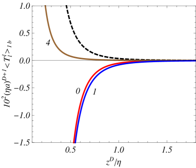
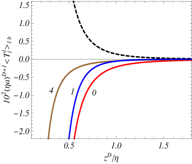
Figure 1: Plate-induced parts in the components of the vacuum energy-momentum tensor as functions of $z^{D}/\eta$ in FRW spacetime with $D=4$. The full curves correspond to the diagonal components and the dashed one is for the energy flux. The numbers near the full curves correspond to the value of the index $l$. For the left plot $c=2/(D+1)$ and for the right one $c=2$.

It is also of interest to consider the time-dependence of the plate-induced parts in the VEVs for an observer with a fixed value of the comoving coordinate $z^{D}$. The corresponding asymptotic expressions at late and early stages of the cosmological expansion can be obtained from those given above for small and large values of $z^{D}/\eta$. For $0<c<1$ and at early stages of the cosmological expansion, $t\rightarrow 0$, we have $\langle T_{\mu}^{\mu}\rangle_{1b}\propto t^{2(1-D)c}$ (no sum over $\mu=0,\ldots,D$), $\langle T_{0}^{D}\rangle_{1b}\propto t^{1-\left(2D-1\right)c}$. In this region, for $D>3$ the energy density is positive for $c<3/D$ and negative for $c>3/D$. At late stages, $t\rightarrow\infty$, the VEVs tend to zero as: $\langle T_{\mu}^{\mu}\rangle_{1b}\propto t^{-c(D+1)}$ (no sum over $\mu=0,\ldots,D-1$), $\langle T_{D}^{D}\rangle_{1b}\propto t^{-c(D-1)-2}$, $\langle T_{0}^{D}\rangle_{1b}\propto t^{-cD-1}$, and the corresponding energy density is negative. In the case $c>1$, the behavior of the VEVs in the limit $t\rightarrow 0$ is as follows: $\langle T_{\mu}^{\mu}\rangle_{1b}\propto t^{-c(D+1)}$ (no sum over $\mu=0,\ldots,D-1$), $\langle T_{D}^{D}\rangle_{1b}\propto t^{-c(D-1)-2}$ and $\langle T_{0}^{D}\rangle_{1b}\propto t^{-cD-1}$. At late stages, $t\rightarrow\infty$, one has: $\langle T_{\mu}^{\mu}\rangle_{1b}\propto t^{-4c}$ (no sum over $\mu=0,\ldots,D$), $\langle T_{0}^{D}\rangle_{1b}\propto t^{1-5c}$. Finally, for models with phantom energy, $c<0$, at early stages of the expansion, corresponding to $t\rightarrow-\infty$, one gets: $\langle T_{\mu}^{\mu}\rangle_{1b}\propto(-t)^{-c(D+1)}$ (no sum over $\mu=0,\ldots,D-1$), $\langle T_{D}^{D}\rangle_{1b}\propto(-t)^{-c(D-1)-2}$ and $\langle T_{0}^{D}\rangle_{1b}\propto(-t)^{-cD-1}$. In this limit the energy density goes to $-\infty$, whereas the limiting values of the normal stress and the energy flux can be either zero or infinity, depending on the value of the parameter $c$. Near the Big Rip, $t\rightarrow 0$, the plate-induced parts tend to zero as: $\langle T_{\mu}^{\mu}\rangle_{1b}\propto(-t)^{-4c}$ (no sum over $\mu=0,\ldots,D$) and $\langle T_{0}^{D}\rangle_{1b}\propto(-t)^{1-5c}$. As we see, for all values of $c$, the plate-induced parts in the VEV of the energy-momentum tensor decay as power-law at late stages of the cosmological expansion. At early stages of the expansion these parts are divergent in models with $c>0$. This is also the case for the energy density in models with $c<0$. In the latter case the energy flux at early stages ($t\rightarrow-\infty$) diverges for $c<-1/D$ and vanishes for $c>-1/D$.

Figure 2 presents the plate-induced part in the energy density ($\beta=\mu=0$, full curves) and the energy flux ($\beta=D$, $\mu=0$, dashed curves) in the model $D=4$, as functions of the comoving time for a fixed value of comoving coordinate $z^{D}$. The numbers near the curves correspond to the values of the parameter $c$ and $H_{0}=H(t_{0})$. For the proper distance from the plate at $t=t_{0}$ we have taken the value $a(t_{0})z^{D}=0.5/H_{0}$.

Figure 2: Plate-induced part in the energy density ($\beta=\mu=0$, full curves) and the energy flux ($\beta=D$, $\mu=0$, dashed curves) in the model $D=4$, as functions of the comoving time for a fixed value of comoving coordinate $z^{D}$. The numbers near the curves correspond to the values of the parameter $c$.

We have considered combined effects of the gravitational field and boundaries on the properties of the quantum vacuum. Another interesting physical effect, arising in time-dependent backgrounds, is the creation of particles. This will give rise to an additional contribution in the expectation value of the energy-momentum tensor which should be added to the VEV we have discussed.

5 The Casimir effect for two conducting plates

For the geometry of two parallel conducting plates we have three separate regions, $z^{D}<0$, $0<z^{D}<L$, and $z^{D}>L$. In the regions $z^{D}<0$ and $z^{D}>L$ the VEVs are the same as for a single conducting plate placed at $z^{D}=0$ and $z^{D}=L$, respectively. In what follows we consider the region between the plates (for the electromagnetic Casimir effect for conducting plates in higher dimensions see, for example, Ref. [34]).

5.1 Field squared

As before, first we consider the VEV of the electric field squared. By using the formula (40) for the two-point function, in the region between the plates, $0<z^{D}<L$, the VEV is presented in the form

$$\langle E^{2}\rangle = \langle E^{2}\rangle_{0}+\frac{8\pi C_{D}}{(\eta a)^{D+1}}\sum_{n=1}^{\infty}\left[D-2(1-u_{n})\partial_{u_{n}}\right]F_{\nu-1}(u_{n})$$ (73)

$$+\frac{4\pi C_{D}}{(\eta a)^{D+1}}\sum_{n=-\infty}^{+\infty}\left[2(1-y_{n})\partial_{y_{n}}-D+2\right]F_{\nu-1}(y_{n}),$$

with the notations

$$u_{n}=1-(nL/\eta)^{2},\;y_{n}=1-(z^{D}-nL)^{2}/\eta^{2}.$$ (74)

The $n=0$ term of the last series is the part in the VEV induced by a single plate at $z^{D}=0$ when the right plate is absent. It coincides with $\langle E^{2}\rangle_{1b}$ given by Eq. (46). Similarly, the $n=1$ term is the VEV induced by a single plate at $z^{D}=L$ when the left plate is absent. This term is obtained from Eq. (46) by the replacement $z^{D}\rightarrow|z^{D}-L|$. The divergences are contained in these two terms only and the remaining part is finite for all $0\leqslant z^{D}\leqslant L$. Consequently, for points near the plates the VEV is dominated by single plate parts.

A simple expression is obtained for $\nu=1/2$:

$$\langle E^{2}\rangle=\langle E^{2}\rangle_{0}+\frac{(D-1)\Gamma\left((D+1)/2\right)}{(4\pi)^{(D-1)/2}(aL)^{D+1}}\left[\zeta(D+1)+\frac{3}{2}\sum_{n=-\infty}^{+\infty}|z^{D}/L-n|^{-D-1}\right],$$ (75)

where $\zeta(x)$ is the Riemann zeta function. The series in this formula is expressed in terms of the Hurwitz zeta function $\zeta(p,x)$ as:

$$\sum_{n=-\infty}^{+\infty}|z^{D}/L-n|^{-D-1}=\zeta(D+1,z^{D}/L)+\zeta(D+1,1-z^{D}/L).$$ (76)

Taking $a=1$, we obtain from Eq. (75) the corresponding VEV for two conducting plates in the Minkowski spacetime. For $D=3$, Eq. (75) gives the VEV for general case of the parameter $c$. In both these cases the plate-induced contribution in the VEV of the electric field squared is positive everywhere.

At short separations between the plates, $L/\eta\ll 1$, the argument of the function $F_{\nu-1}(x)$ is close to 1 and we use the asymptotic formula (29). The leading term of this asymptotic coincides with $F_{1/2}(x)$ and, hence, to the leading order $\langle E^{2}\rangle$ coincides with the corresponding VEV in the case $\nu=1/2$, given by (75): $\langle E^{2}\rangle\approx\langle E^{2}\rangle_{\nu=1/2}$. At large separations, $L/\eta\gg 1$, assuming also that $z^{D},L-z^{D}\gg\eta$, with the help of the asymptotic expression (30), for $\nu\neq 1$ we get

$$\langle E^{2}\rangle \approx \langle E^{2}\rangle_{0}+\frac{2^{2|\nu-1|}(D-1)\Gamma\left(D/2-|\nu-1|+1\right)}{(4\pi)^{D/2}(\eta a)^{D+1}(L/\eta)^{D+2-2|\nu-1|}}\Gamma(|\nu-1|)$$ (77)

$$\times\left[2\left(|\nu-1|-1\right)\zeta(D+2-2|\nu-1|)+\sum_{n=-\infty}^{+\infty}\frac{2-|\nu-1|}{|x^{D}/L-n|^{D+2-2|\nu-1|}}\right].$$

For $\nu=1$ we use Eq. (31). The corresponding asymptotic formula is obtained from Eq. (77) first replacing $\Gamma(|\nu-1|)\rightarrow 4\ln(L/\eta)$ and then putting $\nu=0$. In this case the boundary-induced part of the VEV decays as $\ln(L/\eta)/(L/\eta)^{D+2}$.

For the evaluation of the VEV of the energy-momentum tensor we need also the VEV of the Lagrangian density. By the calculations similar to those for the field squared, in the region between two conducting plates we find

$$\langle F_{\beta\sigma}F^{\beta\sigma}\rangle = \langle F_{\beta\sigma}F^{\beta\sigma}\rangle_{0}+\frac{8\pi C_{D}}{(\eta a)^{D+1}}\left\{2\sum_{n=1}^{\infty}\left[2(1-u_{n})\partial_{u_{n}}-D\right]\left[F_{\nu-1}(u_{n})-F_{\nu}(u_{n})\right]\right.$$ (78)

$$\left.-\sum_{n=-\infty}^{+\infty}\left\{\left[2(1-y_{n})\partial_{y_{n}}+D-4\right]F_{\nu}(y_{n})+\left[2(1-y_{n})\partial_{y_{n}}-D+2\right]F_{\nu-1}(y_{n})\right\}\right\}.$$

The $n=0$ and $n=1$ terms of the last series present the single plate-induced parts for the left and right plates respectively when the other plate is absent.

5.2 Energy-momentum tensor

The VEV of the energy-momentum tensor in the region between the plates is presented in the form

$$\langle T_{\mu}^{\mu}\rangle=\langle T_{\mu}^{\mu}\rangle_{0}+\frac{C_{D}}{2(\eta a)^{D+1}}\left[2\sum_{n=1}^{\infty}g_{\nu}^{(\mu)}(u_{n})+\sum_{n=-\infty}^{\infty}f_{\nu}^{(\mu)}(y_{n})\right],$$ (79)

where $f_{\nu}^{(\mu)}(y)$ is defined in Eq. (57) and we have introduced new functions

$$g_{\nu}^{(0)}(u) = -\left[2(1-u)\partial_{u}-D\right]\left[F_{\nu}(u)+F_{\nu-1}(u)\right],$$

$$g_{\nu}^{(l)}(u) = \left[2\frac{D-3}{D-1}(1-u)\partial_{u}-D+2\right]\left[F_{\nu-1}(u)-F_{\nu}(u)\right]-2F_{\nu}(u),$$ (80)

$$g_{\nu}^{(D)}(u) = \left[2(1-u)\partial_{u}-D+2\right]\left[F_{\nu}(u)+F_{\nu-1}(u)\right]+2\left(D-3\right)F_{\nu}(u),$$

with $l=1,\ldots,D-1$. For the off-diagonal component one has the expression

$$\langle T_{0}^{D}\rangle=-\frac{2s_{\tau}C_{D}L/\eta}{(\eta a)^{D+1}}\sum_{n=-\infty}^{\infty}(z^{D}/L-n)f_{\nu}^{(0D)}(y_{n}),$$ (81)

with the function $f_{\nu}^{(0D)}(y)$ given by Eq. (60). The $n=0$ term in the right-hand side of Eq. (81) gives the energy flux induced by the plate at $z^{D}=0$ when the right plate is absent ($\langle T_{0}^{D}\rangle_{1b}$, see Eq. (59)). Note that the part induced by the right plate, $\langle T_{0}^{D}\rangle-\langle T_{0}^{D}\rangle_{0}-\langle T_{0}^{D}\rangle_{1b}$, vanishes on the surface of the left plate, at $z^{D}=0$. Similarly, the $n=1$ term of the same series presents the energy flux in the geometry of a single plate at $z^{D}=L$. From Eq. (81) it follows that the energy flux, considered as a function of $z^{D}/L$ is antisymmetric with respect to the point $z^{D}/L=1/2$ and, hence, it vanishes at that point.

For $\nu=1/2$ the off-diagonal component vanishes and for the diagonal components we get simpler expressions (no summation over $\mu$)

$$\langle T_{\mu}^{\mu}\rangle=\langle T_{\mu}^{\mu}\rangle_{0}-\frac{(D-1)\Gamma\left((D+1)/2\right)}{2(4\pi)^{(D+1)/2}(aL)^{D+1}}\left[2g_{(0)}^{(\mu)}\zeta(D+1)+\sum_{n=-\infty}^{\infty}\frac{\left(D-3\right)f_{(0)}^{(\mu)}}{|n-z^{D}/L|^{D+1}}\right],$$ (82)

where

$$g_{(0)}^{(\mu)} = 1,\;\mu=0,1,\ldots,D-1,\;g_{(0)}^{(D)}=-D,$$

$$f_{(0)}^{(\mu)} = 1,\;\mu=0,1,\ldots,D-1,\;f_{(0)}^{(D)}=0.$$ (83)

In particular, for $D=3$ the vacuum energy-momentum tensor is uniform in the region between the plates. This is a direct consequence of the conformal invariance of the electromagnetic field in 4-dimensional spacetime.

The expression on the right-hand side of Eq. (82) gives the leading term in the asymptotic expansion of $\langle T_{\mu}^{\mu}\rangle$ for small separations between the plates, $L/\eta\ll 1$, for general value of $\nu$. In the same limit, for the energy flux one has

$$\langle T_{0}^{D}\rangle\approx\frac{|1/2-\nu|(D-1)\Gamma((D+1)/2)}{(4\pi)^{(D+1)/2}(a\eta)^{D+1}(L/\eta)^{D}}\sum_{n=-\infty}^{\infty}\frac{z^{D}/L-n}{|z^{D}/L-n|^{D+1}}.$$ (84)

For large separations between the plates, $L/\eta\gg 1$, and assuming also that $z^{D},L-z^{D}\gg\eta$, for $\nu<1/2$ we have the asymptotic expression (no summation over $\mu$)

$$\langle T_{\mu}^{\mu}\rangle \approx \langle T_{\mu}^{\mu}\rangle_{0}+\frac{2^{1-2\nu}(D-1)\Gamma(1-\nu)\Gamma\left(D/2+\nu\right)}{(4\pi)^{D/2+1}(\eta a)^{D+1}(L/\eta)^{D+2\nu}}$$ (85)

$$\times\left[2r_{\nu}^{(\mu)}\zeta(D+2\nu)+\sum_{n=-\infty}^{\infty}\frac{q_{\nu}^{(\mu)}}{|n-z^{D}/L|^{D+2\nu}}\right],$$

with $q_{\nu}^{(\mu)}$ defined in Eq. (67) and

$$r_{\nu}^{(0)}=-\nu,\;r_{\nu}^{(l)}=\frac{\nu\left(D-3\right)-1}{D-1},\;l=1,\ldots,D-1,\;r_{\nu}^{(D)}=\nu+1.$$ (86)

This asymptotic corresponds to the models with $0<c<1$, describing decelerating expansion.

In the same limit and for $\nu>1/2$ one gets (no sum over $\mu$)

$$\langle T_{\mu}^{\mu}\rangle = \langle T_{\mu}^{\mu}\rangle_{0}+\frac{2^{2\nu-1}(D-1)\Gamma(\nu)\Gamma\left(D/2+1-\nu\right)}{(4\pi)^{D/2+1}(\eta a)^{D+1}(L/\eta)^{D+2-2\nu}}$$ (87)

$$\times\left[2s_{\nu}^{(\mu)}\zeta(D+2-2\nu)+\sum_{n=-\infty}^{\infty}\frac{p_{\nu}^{(\mu)}}{|n-z^{D}/L|^{D+2-2\nu}}\right],$$

where

$$s_{\nu}^{(0)}=\nu-1,\;s_{\nu}^{(l)}=\frac{\left(D-3\right)\left(\nu-2\right)-1}{D-1},\;s_{\nu}^{(D)}=D-\nu-1,$$ (88)

with $l=1,\ldots,D-1$. This corresponds to accelerating expansion with $c>1$ or $c<-1$.

Now let us consider the asymptotic behavior of the energy flux at large separations. By using the asymptotic formula (70), to the leading order we find

$$\langle T_{0}^{D}\rangle=(D-1)\frac{2^{1-2\nu}\Gamma(1-\nu)\Gamma\left(D/2+1+\nu\right)}{(4\pi)^{D/2+1}(\eta a)^{D+1}(L/\eta)^{D+2\nu}}\sum_{n=-\infty}^{\infty}\frac{z^{D}/L-n}{|z^{D}/L-n|^{D+1+2\nu}},$$ (89)

for $\nu<1/2$ (this corresponds to $0<c<1$) and

$$\langle T_{0}^{D}\rangle=\frac{2^{2\nu-1}(D-1)\Gamma(\nu)\Gamma\left(D/2+2-\nu\right)}{(4\pi)^{D/2+1}(\eta a)^{D+1}(L/\eta)^{D+2-2\nu}}\sum_{n=-\infty}^{\infty}\frac{z^{D}/L-n}{|z^{D}/L-n|^{D+3-2\nu}},$$ (90)

for $\nu>1/2$. The latter case corresponds to $c<0$ or $c>1$ with $s_{\tau}=-1$.

In figure 3 we display the boundary-induced parts in the components of the vacuum energy-momentum tensor, $\langle T_{\mu}^{\beta}\rangle_{b}=\langle T_{\mu}^{\beta}\rangle-\langle T_{\mu}^{\beta}\rangle_{0}$, in the region between two plates as functions of $z^{D}/\eta$ for a fixed value of $L/\eta=4$. The graphs are plotted for the FRW model in $D=4$. The full curves correspond to the diagonal components and the numbers near the curves are the values of the index $\beta=\mu$. The dashed curve presents the energy flux. For the left panel $c=2/(D+1)$ and for the right one $c=-3$ (models driven by phantom energy). The graphs for $c=3$ are similar to those for $c=-3$ with the exception that the normal stress ($\beta=\mu=4$) is negative everywhere.

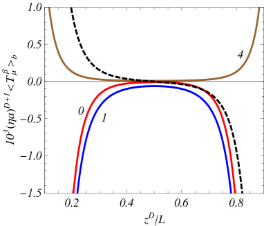
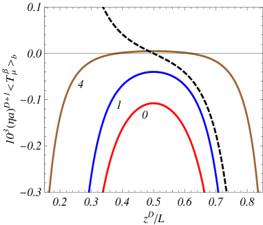
Figure 3: Boundary-induced parts in the components of the vacuum energy-momentum tensor in the region between two conducting plates, as functions of $z^{D}/\eta$ for a fixed value of $L/\eta=4$. The graphs are plotted for the FRW model in $D=4$. The full curves correspond to the diagonal components and the numbers near the curves are the values of the index $\beta=\mu$. The dashed curves present the energy flux. For the left panel $c=2/(D+1)$ and for the right one $c=-3$.

5.3 The Casimir force

The Casimir force acting on the plate can be obtained evaluating the normal stress on the surface of the plate. Due to the symmetry of the problem the forces acting on the left and right plates are equal in magnitude. For the effective pressure $P$ on the plate at $z^{D}=0$ one has $P=-\langle T_{D}^{D}\rangle_{z^{D}=0}$. The corresponding force is decomposed into the self action and interaction parts. The self action part comes from the stress $\langle T_{D}^{D}\rangle_{1}$. For $D>3$ this part is divergent on the plate. However, because of the symmetry of the problem, the self-forces from the left- and right-hand sides of the plate compensate each other and the corresponding net force vanishes. The interaction part of the vacuum pressure on the plate is directly obtained from the second term in the right-hand side of Eq. (79) for $\langle T_{D}^{D}\rangle$ omitting the term $n=0$ in the second summation (the latter corresponds to the self action force). In this way, by taking into account that for $z^{D}=0$ we have $y_{n}=u_{n}$, for the interaction part of the Casimir pressure one finds

$$P^{\mathrm{(int)}}=-\frac{4C_{D}}{(\eta a)^{D+1}}\sum_{n=1}^{\infty}\left\{\left[(1-u_{n})\partial_{u_{n}}-1\right]F_{\nu}(u_{n})+F_{\nu-1}(u_{n})/2\right\}.$$ (91)

In the special case $\nu=1/2$, this expression is simplified to

$$P^{\mathrm{(int)}}=-\frac{D(D-1)\Gamma\left((D+1)/2\right)}{(4\pi)^{(D+1)/2}(aL)^{D+1}}\zeta(D+1).$$ (92)

This pressure is negative and corresponds to the attractive force. In particular, for $a=1$ Eq. (92) gives the Casimir force for the plates in the $(D+1)$-dimensional Minkowski spacetime.

The expression (92) describes the asymptotic behavior of the Casimir pressure at small separations in general case of $\nu$:

$$P^{\mathrm{(int)}}\approx P_{\nu=1/2}^{\mathrm{(int)}},\;L/\eta\ll 1.$$ (93)

At large separations between the plates, $L/\eta\gg 1$, the dominant contribution to the Casimir force comes from the term in Eq. (91) with the function $F_{\nu-1}(u_{n})$ for $\nu<1/2$ and from the term with $F_{\nu}(u_{n})$ for $\nu>1/2$. By making use of the asymptotic expressions for these functions, to the leading order we get

$$P^{\mathrm{(int)}}\approx-\frac{2^{2-2\nu}(D-1)\Gamma(1-\nu)\Gamma\left(D/2+\nu\right)}{(4\pi)^{D/2+1}(\eta a)^{D+1}(L/\eta)^{D+2\nu}}\zeta(D+2\nu),$$ (94)

for $\nu<1/2$ and

$$P^{\mathrm{(int)}}\approx-\frac{2^{2\nu}(D-1)\left(D-2\nu\right)\Gamma(\nu)}{(4\pi)^{D/2+1}(\eta a)^{D+1}(L/\eta)^{D+2-2\nu}}\Gamma\left(D/2+1-\nu\right)\zeta(D+2-2\nu),$$ (95)

for $\nu>1/2$. In deriving the asymptotics (94) and (95) we have assumed that $(L/\eta)^{|2\nu-1|}\gg 1$ and these asymptotics are not valid for $\nu$ too close to 1/2. Recall that for $\nu=1/2$ we have the simple expression (92). Note that in all these cases the effective pressure $P^{\mathrm{(int)}}$ is negative for $\nu<D/2$ and the corresponding vacuum forces are attractive. For $D<2\nu<D+1$ (the right condition comes from Eq. (41)), the Casimir pressure becomes positive and the corresponding forces are repulsive at large separations. This corresponds to the values of the parameter $c$ in the range

$$D/3<c<(D-1)/2.$$ (96)

Hence, in the range of powers (96), the Casimir force is attractive at small separations and repulsive at large separations. This means that at some intermediate value for $L$ the force vanishes. This corresponds to an unstable equilibrium point. Note that, in the range (96), though the two-point function for the field tensor contains no infrared divergences, the latter are contained in the two-point function for the vector potential. In both cases of Eqs. (94) and (95), the decay of the Casimir forces with the distance between the plates is slower than in the case of the Minkowski bulk.

For a fixed value of a comoving separation between the plates, $L$, the asymptotic behavior of the Casimir force, as a function of the comoving time, is obtained from Eqs. (94) and (95). For $0<c<1$, at early and late stages of the cosmological expansion one has $P^{\mathrm{(int)}}\propto t^{-2\left(D-1\right)c}$, $t\rightarrow 0$, and $P^{\mathrm{(int)}}\propto t^{-c(D+1)}$, $t\rightarrow\infty$. In the case $c>1$, the asymptotics are given by $P^{\mathrm{(int)}}\propto t^{-c(D+1)}$ for $t\rightarrow 0$ and $P^{\mathrm{(int)}}\propto t^{-4c}$ for $t\rightarrow\infty$. And finally, in the models driven by phantom energy, $c<0$, the Casimir force behaves as $P^{\mathrm{(int)}}\propto(-t)^{-c(D+1)}$ for $t\rightarrow-\infty$ and $P^{\mathrm{(int)}}\propto(-t)^{-4c}$ for $t\rightarrow 0$. In all cases, the force tends to zero at late times and diverges at early times.

In order to display the influence of the gravitational field on the Casimir force, in figure 4 we present the ratio $P^{\mathrm{(int)}}/P_{\nu=1/2}^{\mathrm{(int)}}$ as a function of $L/\eta$ and of the parameter $c$ in the FRW model with $D=4$. Note that $P^{\mathrm{(int)}}/P_{\nu=1/2}^{\mathrm{(int)}}$ is the ratio of the Casimir pressure in FRW spacetime to the corresponding pressure for the plates in the Minkowski spacetime with the separation equal to the proper distance $aL$. The left and right plots correspond to the range of powers $c<D/(2D-3)$ and $c>D/3$ (see Eq. (41)), respectively. At small separations the effects of the curvature are small and we have $P^{\mathrm{(int)}}/P_{\nu=1/2}^{\mathrm{(int)}}\approx 1$. As it is seen from the graphs, at separations larger than the curvature radius of the background spacetime the curvature effects are essential. In particular, in models with power law inflation, depending on the values of the parameter $c$, the force can change the sign becoming repulsive.

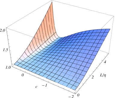
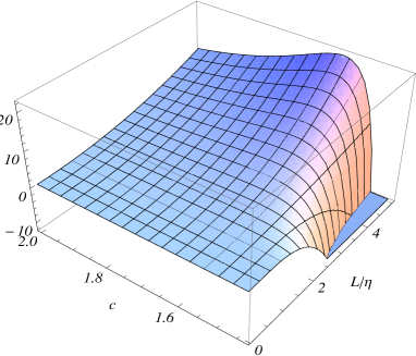
Figure 4: Ratio $P^{\mathrm{(int)}}/P_{\nu=1/2}^{\mathrm{(int)}}$ as a function of $L/\eta$ and of the parameter $c$ in the FRW model with $D=4$. The left and right plots correspond to the range of powers $c<D/(2D-3)$ and $c>D/3$.

6 Conclusion

In this paper we have considered the electromagnetic field two-point functions in a fixed spatially flat $(D+1)$-dimensional FRW background with a power law scale factor (1). As a special case the latter includes the models of extended inflation ($c>1$) and the models driven by phantom energy ($c<0$). For the evaluation of the two-point functions the direct mode summation approach is employed. In this approach a complete set of mode functions for the vector potential are needed and they are presented in section 2, Eq. (10). We assume that the field is prepared in the Bunch-Davies vacuum state. In the boundary-free geometry, the corresponding two-point function for the vector potential is given by Eq. (21). The integral representation of this function is infrared convergent under the condition (18) for the parameter $c$. Though we have no closed expression for the integral in the right-hand side of Eq. (21), it does not contribute to the two-point function for the field tensor and, hence, to the VEVs of the field squared and the energy-momentum tensor. We provided closed expressions, Eq. (23), for the two-point function of the field tensor. This function is infrared convergent for the values of the parameter $c$ in the range (26). For the values of $c$ outside this range the Bunch-Davies vacuum in a boundary-free FRW background is not a physically realizable state.

The two-point functions for the geometry of two parallel perfectly conducting plates are considered in section 3. The corresponding mode functions are given by Eq. (33) and the two-point functions are expressed in terms of the boundary-free two-point functions by Eqs. (38) and (40). The two-point function of the field tensor for the Bunch-Davies vacuum state is infrared convergent under the condition (41) for the expansion parameter. This function can be used for the investigation of the VEVs of the field squared and the energy-momentum tensor. First we have considered the geometry of a single conducting plate. The corresponding VEVs are decomposed into the boundary-free and plate-induced contributions. For points outside the plate, the divergences in the VEVs are the same as in the boundary-free geometry and the renormalization is reduced to the one for the boundary-free parts in the VEVs. The plate-induced contributions are finite and they are directly obtained from the corresponding part in the two-point function for the field tensor taking the coincidence limit. These contributions depend on the coordinate $z^{D}$, normal to the plate, in the combination $z^{D}/|\tau|$ with $\tau$ being the conformal time coordinate. Up to a constant factor, this combination coincides with the ratio of the proper distance from the plate to the curvature radius of the background spacetime. Simple expressions for the VEVs are obtained for $\nu=1/2$. This possibility is realized in two special cases: (i) $c=0$ and $D$ is arbitrary, corresponding to $(D+1)$-dimensional Minkowski spacetime, and (ii) $D=3$ for general $c$. In $D=3$ the electromagnetic field is conformally invariant and in this case the expressions for the Casimir densities in the geometry under consideration are obtained from those for the Minkowskian bulk by conformal transformation.

In the geometry of a single plate, the boundary-induced part in the VEV of the electric field squared is given by Eq. (46). At small proper distances from the plate, compared with the curvature radius of the background spacetime, the effects of the gravitational field are small and to the leading order the plate-induced part coincides with the corresponding result for a plate in Minkowski spacetime. In this region the plate-induced part in the VEV of the electric field squared is positive and it dominates in the total VEV. At large distances from the plate, the leading terms in the corresponding asymptotic expansion are given by Eqs. (51) and (52) for the cases $\nu\neq 1$ and $\nu=1$ respectively. Depending on the expansion parameter and on the spatial dimension, in this region the plate-induced part in the VEV of the electric field squared can be either negative or positive.

For the geometry of a single plate, the boundary-induced contributions in the VEVs of the diagonal components of the energy-momentum tensor are given by Eqs. (56), (57). Note that, unlike to the case of a plate in the Minkowski spacetime, in the problem under consideration the stresses along the directions parallel to the plate are not equal to the energy density. In addition to the diagonal components, the vacuum energy-momentum tensor has also a nonzero off-diagonal component which corresponds to the energy flux along the direction normal to the plate. The boundary-free part in the VEV of the energy-momentum tensor is diagonal and the energy flux is purely boundary-induced effect. For points near the plate, the leading terms in the asymptotic expansion of the energy-momentum tensor components are given by Eqs. (64) and (65). In this region the energy density and the parallel stresses are negative and the off-diagonal component $\langle T_{0}^{D}\rangle_{1b}$ is positive. The latter means that the energy flux is directed from the plate. The normal stress is positive in models with decelerating expansion and negative for accelerating expansion. At large proper distances from the plate compared with the curvature radius of the background spacetime, the leading terms in the plate-induced VEVs are given by Eqs. (66), (71) in the case of decelerated expansion and by Eqs. (68), (72) in the case of accelerated expansion. In both cases, the decay of the plate-induced parts in the energy density and in the parallel stresses, as functions of the distance from the plate, is slower than in the corresponding problem on Minkowski bulk. Depending on the value of the expansion parameter, the plate-induced contribution in the energy density can be either negative or positive. The energy flux is always directed from the plate. For a fixed value of the comoving coordinate $z^{D}$, at late times of the cosmological expansion, the plate-induced parts in the VEV of the energy-momentum tensor decay as power-law. In particular, the energy density decays as $t^{-(D+1)c}$ in models with decelerated expansion ($0<c<1$) and like $|t|^{-4c}$ for an accelerated expansion.

In the region between two parallel conducting plates the VEVs are decomposed as Eqs. (73), (79), and (81) for the field squared and the energy-momentum tensor, respectively. The $n=0$ and $n=1$ terms in the last series of these representations correspond to the single plate parts (left and right, respectively) when the second plate is absent. The surface divergences are contained in these terms only and the remained part is finite on the plates. Single plate parts dominate near the plates. The energy flux, considered as a function of $z^{D}$, is antisymmetric with respect to the point $z^{D}=L/2$. It is directed from the left plate for $0<z^{D}<L/2$ and from the right plate for $L/2<z^{D}<L$ and vanishes at $z^{D}=L/2$. We have provided simple asymptotic expressions of the VEVs for small and large separations between the plates. For the geometry of a single plate the Casimir normal stresses on the left- and right-hand sides are the same and the net force acting on the plate vanishes. The presence of the second plate induces a force referred here as an interaction force. The latter, acting on the left plate, is obtained putting $z^{D}=0$ in the part of the normal stress induced by the right plate. The corresponding effective pressure is given by Eq. (91). At small separations between the plates, the spacetime curvature effects are subdominant and to the leading order we recover the result for the plates in the Minkowski spacetime, Eq. (92). In this limit the forces are attractive. At larger separations, the asymptotics of the Casimir forces are given by Eqs. (94) and (95) for decelerated and accelerated expansions respectively. The corresponding forces are attractive except the range of powers (96), where the Casimir pressure becomes positive at large separations and the corresponding forces are repulsive. In this range for the values of the parameter $c$, though the two-point function of the field tensor contains no infrared divergences, the latter are contained in the two-point function for the vector potential.

References

• [1] N.D. Birrel and P.C.W. Davies, Quantum Fields in Curved Space (Cambridge University Press, Cambridge, 1982); A.A. Grib, S.G. Mamayev, and V.M. Mostepanenko, Vacuum Quantum Effects in Strong Fields (Friedmann Laboratory Publishing, St. Petersburg, 1994); L. Parker and D. Toms, Quantum Field Theory in Curved Spacetime: Quantized Fields and Gravity (Cambridge University Press, Cambridge, 2009).
• [2] D. Boyanovsky, H.J. de Vega, and R. Holman, Phys. Rev. D 49, 2769 (1994); D. Boyanovsky, H.J. de Vega, R. Holman, D.-S. Lee, and A. Singh, Phys. Rev. D 51, 4419 (1995).
• [3] G. Esposito, G. Miele, L. Rosa, and P. Santorelli, Class. Quantum Grav. 12, 2995 (1995).
• [4] H. Kleinert and A. Zhuk, Theor. Math. Phys. 108, 1236 (1996); A. Zhuk and H. Kleinert, Theor. Math. Phys. 109, 1483 (1996).
• [5] M. Bordag, J. Lindig, V.M. Mostepanenko, and Yu.V. Pavlov, Int. J. Mod. Phys. D 6, 449 (1997); M. Bordag, J. Lindig, and V.M. Mostepanenko, Class. Quantum Grav. 15, 581 (1998).
• [6] S.A. Ramsey and B.L. Hu, Phys. Rev. D 56, 678 (1997).
• [7] S.P. Gavrilov, D.M. Gitman, and S.D. Odintsov, Int. J. Mod. Phys. A 12, 4837 (1997).
• [8] P.R. Anderson and W. Eaker, Phys. Rev. D 61, 024003 (1999).
• [9] S. Habib, C. Molina-ParΓ­s, and E. Mottola, Phys. Rev. D 61, 024010 (1999).
• [10] C. Molina-ParΓ­s, P.R. Anderson, and S.A. Ramsey, Int. J. Theor. Phys. 40, 2231 (2001).
• [11] E. Elizalde, J. Phys. A 39, 6299 (2006).
• [12] C.A.R. Herdeiro and M. Sampaio, Class. Quantum Grav. 23, 473 (2006).
• [13] V.B. Bezerra, G.L. Klimchitsaya, V.M. Mostepanenko, C. Romero, Phys. Rev. D 83, 104042 (2011); V.B. Bezerra, V.M. Mostepanenko, H.F. Mota, C. Romero, Phys. Rev. D 84, 104025 (2011).
• [14] A.D. Linde, Particle Physics and Inflationary Cosmology (Harwood Academic Publishers, Chur, Switzerland, 1990).
• [15] E. Elizalde, S.D. Odintsov, A. Romeo, A.A. Bytsenko, and S. Zerbini, Zeta Regularization Techniques with Applications (World Scientific, Singapore, 1994); V.M. Mostepanenko and N. N. Trunov, The Casimir Effect and Its Applications (Clarendon, Oxford, 1997); K.A. Milton, The Casimir Effect: Physical Manifestation of Zero-Point Energy (World Scientific, Singapore, 2002); M. Bordag, G.L. Klimchitskaya, U. Mohideen, and V.M. Mostepanenko, Advances in the Casimir Effect (Oxford University Press, Oxford, 2009); Lecture Notes in Physics: Casimir Physics, edited by D. Dalvit, P. Milonni, D. Roberts, and F. da Rosa (Springer, Berlin, 2011), Vol. 834.
• [16] W. Goldberger and I. Rothstein, Phys. Lett. B 491, 339 (2000); S. Nojiri, S.D. Odintsov, and S. Zerbini, Class. Quantum Grav. 17, 4855 (2000); A. Flachi and D.J. Toms, Nucl. Phys. B 610, 144 (2001); J. Garriga, O. PujolΓ s, and T. Tanaka, Nucl. Phys. B 605, 192 (2001); E. Elizalde, S. Nojiri, S.D. Odintsov, and S. Ogushi, Phys. Rev. D 67, 063515 (2003); A.A. Saharian and M.R. Setare, Phys. Lett. B 584, 306 (2004); A. Flachi, A. Knapman, W. Naylor, and M. Sasaki, Phys. Rev. D 70, 124011 (2004); E. Elizalde, S. Nojiri, S.D. Odintsov, and P. Wang, Phys. Rev. D 71, 103504 (2005); M. Frank, I. Turan, and L. Ziegler, Phys. Rev. D 76, 015008 (2007); L.P. Teo, Phys. Lett. B 682, 259 (2009); H. Cheng, arXiv:0904.4183; L.P. Teo, arXiv:1305.6348.
• [17] A. Knapman and D.J. Toms, Phys. Rev. D 69, 044023 (2004); A.A. Saharian, Nucl. Phys. B 712, 196 (2005); A.A. Saharian, Phys. Rev. D 70, 064026 (2004); A.A. Saharian and A.L. Mkhitaryan, J. High Energy Phys. 08 (2007) 063; E. Elizalde, S.D. Odintsov, and A.A. Saharian, Phys. Rev. D 87, 084003 (2013).
• [18] A. Flachi, J. Garriga, O. PujolΓ s, and T. Tanaka, J. High Energy Phys. 08 (2003) 053; A. Flachi and O. PujolΓ s, Phys. Rev. D 68, 025023 (2003); A.A. Saharian, Phys. Rev. D 73, 044012 (2006); A.A. Saharian, Phys. Rev. D 73, 064019 (2006); A.A. Saharian, Phys. Rev. D 74, 124009 (2006); E. Elizalde, M. Minamitsuji, and W. Naylor, Phys. Rev. D 75, 064032 (2007); R. Linares, H.A. Morales-TΓ©cotl, and O. Pedraza, Phys. Rev. D 77, 066012 (2008); M. Frank, N. Saad, and I. Turan, Phys. Rev. D 78, 055014 (2008); E. Elizalde, S.D. Odintsov, and A.A. Saharian, Phys. Rev. D 79, 065023 (2009).
• [19] A.A. Saharian and T.A. Vardanyan, Class. Quantum Grav. 26, 195004 (2009); E. Elizalde, A.A. Saharian, and T.A. Vardanyan, Phys. Rev. D 81, 124003 (2010); A.A. Saharian, Int. J. Mod. Phys. A 26, 3833 (2011); K.A. Milton and A.A. Saharian, Phys. Rev. D 85, 064005 (2012).
• [20] M.R. Setare and R. Mansouri, Class. Quantum Grav. 18, 2331 (2001); M.R. Setare, Class. Quantum Grav. 18, 4823 (2001); P. Burda, JETP Lett. 93, 632 (2011).
• [21] A.A. Saharian, A.S. Kotanjyan, and H.A. Nersisyan, arXiv:1307.5536.
• [22] A.A. Saharian and M.R. Setare, Phys. Lett. B 659, 367 (2008); S. Bellucci and A.A. Saharian, Phys. Rev. D 77, 124010 (2008); A.A. Saharian, Class. Quantum Grav. 25, 165012 (2008); E.R. Bezerra de Mello and A.A. Saharian, J. High Energy Phys. 12 (2008) 081; S. Bellucci, A.A. Saharian, and H.A. Nersisyan, Phys. Rev. D 88, 024028 (2013).
• [23] T.S. Bunch and P.C.W. Davies, J. Phys. A 11, 1315 (1978).
• [24] L.H. Ford and L. Parker, Phys. Rev. D 16, 245 (1977); T.S. Bunch and P.C.W. Davies, Proc. Roy. Soc. London A 356, 569 (1977); S.G. Mamaev, Theor. Math. Phys. 42, 229 (1980); L.H. Ford and D.J. Toms, Phys. Rev. D 25, 1510 (1982); A. Vilenkin and L.H. Ford, Phys. Rev. D 26, 1231 (1982); C. Pathinayake and L.H. Ford, Phys. Rev. D 37, 2099 (1988); V.B. Bezerra, V.M. Mostepanenko, and C. Romero, Grav. Cosmol. 2, 206 (1996); A.A. Saharian and A.L. Mkhitaryan, Eur. Phys. J. C 66, 295 (2010).
• [25] A.A. Saharian and M.R. Setare, Phys. Lett. B 687, 253 (2010); A.A. Saharian and M.R. Setare, Class. Quantum Grav. 27, 225009 (2010).
• [26] F. Lucchin and S. Matarrese, Phys. Rev. D 32, 1316 (1985); L.F. Abbott and M.B. Wise, Nucl. Phys. B 244, 541 (1987).
• [27] D. La and P.J. Steinhardt, Phys. Rev. Lett. 62, 376 (1989); D. La and P.J. Steinhardt, Phys. Lett. B 220, 375 (1989).
• [28] A.B. Burd and J.D. Barrow, Nucl. Phys. B 308, 929 (1988).
• [29] K.I. Maeda, Phys. Rev. D 37, 858 (1988); S. Kotsakis and P.J. Saich, Class. Quantum Grav. 11, 383 (1994).
• [30] B. Allen and T. Jacobson, Commun. Math. Phys. 103, 669 (1986).
• [31] A.P. Prudnikov, Yu.A. Brychkov, and O.I. Marichev, Integrals and Series (Gordon and Breach, New York, 1986), Vol. 2.
• [32] Handbook of Mathematical Functions, edited by M. Abramowitz and I.A. Stegun (Dover, New York, 1972).
• [33] J. AmbjΓΈrn and S. Wolfram, Ann. Phys. 147, 1 (1983).
• [34] H. Alnes, K. Olaussen, F. Ravndal, and I.K. Wehus, J. Phys. A: Math. Theor. 40, F315 (2007); A. Edery and V.N. Marachevsky, J. High Energy Phys. 12 (2008) 035; L.P. Teo, J. High Energy Phys. 10 (2010) 019; L.P. Teo, Phys. Rev. D 83, 105020 (2011).