Spin $1/2$ quasinormal mode frequencies in Schwarzschild-AdS spacetime

Abstract

We find the asymptotic formula for quasinormal mode frequencies $\omega_{n}$ of the Dirac equation in a Schwarzschild-AdS_D background in space-time dimension $D>3$, in the large black-hole limit appropriate to many applications of the AdS/CFT correspondence. By asymptotic, we mean large overtone number $n$ with everything else held fixed, and we find the $O(n^{0})$ correction to the known leading $O(n)$ behavior of $\omega_{n}$. The result has the schematic form $\omega_{n}\simeq n\,\Delta\omega+A\,\ln n+B$, where $\Delta\omega$ and $A$ are constants and $B$ depends logarithmically on the $(D-2)$-dimensional spatial momentum ${\bm{k}}$ parallel to the horizon. We show that the asymptotic result agrees well with exact quasinormal mode frequencies computed numerically.

I Introduction and Results

I.1 Overview

There has been a great deal of numerical and analytic work on quasinormal modes of black holes. (For some modern reviews, see Refs. QNMreview1 ; QNMreview2 .) Because of gauge-gravity duality, one case of particular interest over the last decade has been that of black holes in asymptotically anti-de Sitter spacetimes. In this case, low-lying quasinormal mode frequencies can be related to the poles of Green functions Birmingham ; SonStarinets ; Starinets ; KovtunStarinets and so to the long distance exponential fall-off of various correlators in certain finite-temperature and finite-density field theories. Also, the full set of quasinormal frequencies can be related to functional determinants in the gravity theory, which are dual to ‘$1/N$’ corrections to strongly-coupled field theories DHS ; DHS0 . Except in a few special cases, exact computation of quasinormal modes requires numerics. But it is generally possible, using WKB-like methods, to obtain analytic results for quasinormal mode frequencies $\omega_{n}$ in the limit of large overtone number $n$ — that is, in the limit of large $|\omega_{n}|$. In most cases, quasinormal mode frequencies are evenly spaced at large $n$, with asymptotic expansion

$$\omega_{n}\approx n\,\Delta\omega+\mbox{constant}+\cdots,$$ (1)

where $\Delta\omega$ is the asymptotically constant spacing between successive $\omega_{n}$. In most cases, the asymptotic expansion has been computed analytically to at least $O(n^{0})$, so as to include the constant term on the right-hand side of (1). In this paper, we focus on the limit where $n$ is taken large while holding other quantities fixed (such as mass $m$ and spatial momentum ${\bm{k}}$ parallel to the horizon).

The goal of the present paper is to fill one gap in the literature concerning such asymptotic formulas for $\omega_{n}$. To our knowledge, nobody has previously analyzed analytically the case of quasinormal modes of half-integer spin fields in Schwarzschild-AdS (SAdS) spacetimes through $O(n^{0})$, except in the special low-dimensional case of BTZ black holes BTZblackhole (in bulk space-time dimension $D{=}3$), where exact analytic results for all $\omega_{n}$ may be found BTZdirac . In this paper, we specialize to the case of spin-$\tfrac{1}{2}$ fields in SAdS_D with $D>3$. We will find a result that has the schematic form

$$\omega_{n}\approx n\,\Delta\omega+A\ln n+B+\cdots,$$ (2)

and we will evaluate all the terms through $O(n^{0})$. An interesting and unusual feature here is the $\ln n$ term. Such dependence on $\ln n$ does not arise for quasinormal modes of asymptotically flat black holes (see MusiriSiopsis:Dirac for an analysis of the spin-$\tfrac{1}{2}$ case), nor does it arise in the analysis of spin-0 or spin-2 quasinormal modes of SAdS NatarioSchiappa ; CardosoNatarioSchiappa ; MusiriNessSiopsis . However, a logarithmic dependence has been found for spin-1 quasinormal modes of SAdS for $D{=}4$ MusiriNessSiopsis . Our result shows that the spin-$\tfrac{1}{2}$ case has a logarithm in all dimensions $D>3$. We will verify our result by comparison to (i) existing numerical results for the special case of massless Dirac fermions in $D{=}4$ GiammatteoJing and (ii) our own numeric calculations for massive Dirac fermions in $D{=}5$.

We note in passing that the case of massive spin-$\tfrac{1}{2}$ fields in SAdS arises naturally in the duality between strongly-coupled ${\cal N}{=}4$ super Yang-Mills theory and Type IIB supergravity on AdS${}_{5}\times S^{5}$ (or SAdS${}_{5}\times S^{5}$ for finite temperature) because the Kaluza-Klein reduction on $S^{5}$ gives mass to all spin-$\tfrac{1}{2}$ fields in (S)AdS₅ KRvN .

For the sake of simplicity of discussion and of AdS/CFT applications to infinite-volume systems, we will focus on black branes, which correspond to the limiting case of arbitrarily “large” black holes. In the remainder of this introduction, we review the corresponding metric and set up our choice of coordinates, and then we summarize our analytic results for the asymptotic quasinormal mode frequencies. The derivation is given in section II. In section III, we explain our numerical method for computing exact quasinormal mode frequencies in the massive case. Finally, comparison of our asymptotic formulas to both our own numerics and the numerics of ref. GiammatteoJing is given in section IV, and the $\log(n)$ term in the expansion (2) is verified.

As mentioned earlier, in this paper we study the limit of large overtone number $n$ with all other parameters held fixed. Readers interested in other limits may find a discussion of large chemical potential $\mu$ in HerzogRen (with specific calculations in a probe approximation). Also, in the case of scalar rather than spin-$\tfrac{1}{2}$ fields, a discussion of large mass $m$ may be found in refs. largem1 ; largem2 and large momentum ${\bm{k}}$ in ref. largek .

I.2 Metric

Two standard, equivalent forms of the SAdS_D black-brane metric in $D$ space-time dimensions are

$$ds^{2}=\frac{L^{2}}{z^{2}}\left[-f\,dt^{2}+d{\bm{x}}^{2}+f^{-1}dz^{2}\right]$$ (3a)

and

$$ds^{2}=-F\,dt^{2}+r^{2}\,\frac{d{\bm{x}}^{2}}{L^{2}}+F^{-1}dr^{2},$$ (3b)

where $L$ is the radius associated with the asymptotic AdS space-time,

$$z=\frac{L^{2}}{r}\,,$$ (4)

$$f\equiv 1-\Bigl{(}\frac{r_{\rm h}}{r}\Bigr{)}^{D-1}=1-\Bigl{(}\frac{z}{z_{\rm h}}\Bigr{)}^{D-1},$$ (5a)

and

$$F\equiv\frac{r^{2}f}{L^{2}}=\frac{L^{2}f}{z^{2}}\,.$$ (5b)

The boundary of AdS is at $z=0$ and $r=\infty$, the black hole horizon is at $z=z_{\rm h}$ and $r=r_{\rm h}$, and the singularity is at $z=\infty$ and $r=0$. (Since both $z$ and $r$ are common variable choices, depending on context, we will occasionally jump back and forth between them in order to facilitate comparison of formulas with the rest of the literature on quasinormal modes.)

We will consider fermions of mass $m$ propagating in this metric background. In applications of gauge-gravity duality, masses $m$ of the spin-$\tfrac{1}{2}$ fields in the gravity theory are related by duality to conformal dimensions $\Delta$ of spin-$\tfrac{1}{2}$ operators in the field theory by $|mL|=\Delta-\frac{1}{2}(D-1)$ MAGOO .

I.3 Asymptotic Results

The result we find in this paper for (retarded) quasinormal mode frequencies of massive spin $\tfrac{1}{2}$ fermions in SAdS is

$$\frac{\omega_{n\pm}}{\pi T}\simeq 4e^{-i\pi/(D-1)}\sin\Bigl{(}\frac{\pi}{D-1}\Bigr{)}\\ \times\left[n-\frac{i}{2\pi}\ln\left(\frac{n^{a}}{|{\bm{k}}|/\pi T}\right)+\tfrac{1}{2}(|mL|-1\pm\tfrac{1}{2})+\frac{(D-3)^{2}}{8(D-1)(D-2)}+\frac{i\xi}{\pi}\right]$$ (6)

(massive Dirac fermion, $$D>3$$),

where ${\bm{k}}$ is the $(D{-}2)$-dimensional spatial momentum conjugate to ${\bm{x}}$ in (3),

$$T=\frac{(D-1)r_{\rm h}}{4\pi L^{2}}=\frac{(D-1)}{4\pi z_{\rm h}}$$ (7)

is the Hawking temperature of the black hole,

$$\xi\equiv-\frac{a}{2}\ln\left(4\sin\Bigl{(}\frac{\pi}{D-1}\Bigr{)}\right)+\frac{(1-a)}{2}\ln(1-a)+\frac{1}{2}\ln\bigl{[}\Gamma(a)\sin(\pi a)\bigr{]},$$ (8)

and

$$a\equiv\frac{(D-3)}{2(D-2)}\,.$$ (9)

We assume ${\bm{k}}\not=0$ here and throughout. The leading $O(n)$ piece of our result (6) was known previously from numerical results on the asymptotic spacing between modes for massless spin-$\frac{1}{2}$ fermions in $D{=}4$ GiammatteoJing and is the same for general $D$ as the leading $O(n)$ result for fields of other spin MusiriSiopsis:AdS ; MusiriNessSiopsis ; NatarioSchiappa . Some authors adopt the convention of studying advanced rather than retarded quasinormal modes (outgoing rather than infalling boundary condition at the horizon), which corresponds to taking the complex conjugate of our result.

The $\pm$ sign in (6) distinguishes different spin states, in a way to be made precise later. The formula (6) only shows the quasinormal mode frequencies $\omega=\omega_{n\pm}$ in the right-half complex plane. The corresponding quasinormal frequencies in the left-hand plane are given by $\omega=-\omega_{n\mp}^{*}$.

For $D{=}5$, our result specializes to

$$\frac{\omega_{n\pm}}{\pi T}\simeq 2(1-i)\left[n-\frac{i}{2\pi}\ln\left(\frac{n^{1/3}}{|{\bm{k}}|/\pi T}\right)+\tfrac{1}{2}(|mL|-1\pm\tfrac{1}{2})+\frac{1}{24}+\frac{i\xi_{5}}{\pi}\right]$$ (10)

(massive Dirac fermion, $$D=5$$),

with

$$\xi_{5}=\tfrac{1}{2}\ln\Gamma(\tfrac{1}{3})-\tfrac{1}{12}\ln 3-\tfrac{5}{12}\ln 2=0.112348.$$ (11)

Henceforth, we will assume that $m$ is chosen by convention to be positive, and so we will drop the absolute value signs in (6) and elsewhere. Fig. 1 gives a first look at the comparison of our numerical results (described later) for exact quasi-normal mode frequencies and the asymptotic formula (10) for $D{=}5$, $mL=\tfrac{1}{2}$, and two different values of $|{\bm{k}}|$. We will make more precise comparisons later on.

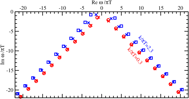
Figure 1: Retarded quasi-normal mode frequencies in the complex $\omega$ plane for $D{=}5$, $mL=\tfrac{1}{2}$, and spin states with ${\bm{\sigma}}\cdot{\bm{\hat{}}{\bm{k}}}=+1$ (as defined in section II.1). Note that the figure is not left-right symmetric. The result for ${\bm{\sigma}}\cdot{\bm{\hat{}}{\bm{k}}}=-1$ is the left-right mirror image of this figure, as required by parity. The red circles are numerical results for $|{\bm{k}}|/\pi T=0.3$, and the blue squares are those for $|{\bm{k}}|/\pi T=2.3$. The correspondingly colored crosses show the asymptotic formula (10).

Massless fermions are a special case and require a careful discussion of boundary conditions, to be given later. Massless fermions have previously been studied numerically by Giammatteo and Jing GiammatteoJing in $D{=}4$. We will find that, for their choice of boundary conditions, the analytic result for large $n$ happens to be given by the same mathematical formula as (6) if you plug in $|mL|=\tfrac{3}{2}$ instead of the naive choice $|mL|=0$. For comparison to the $D{=}4$ simulations of Giammatteo and Jing, whose numerical results are for the case we call $\omega_{n+}$ in the lower-right complex plane, our result is then

$$\frac{\omega_{n+}}{\pi T}\simeq e^{-i\pi/3}2\sqrt{3}\left[n-\frac{i}{2\pi}\ln\left(\frac{n^{1/4}}{|{\bm{k}}|/\pi T}\right)+\frac{25}{48}+\frac{i\xi_{4}}{\pi}\right]$$ (12)

(massless Dirac fermion, $$D=4$$),

with

$$\xi_{4}=\tfrac{1}{2}\ln\Gamma(\tfrac{1}{4})+\tfrac{5}{16}\ln 3-\tfrac{9}{8}\ln 2=0.207537\,.$$ (13)

II Derivation

II.1 The Dirac equation

The Dirac equation in curved space is

$$\Gamma^{M}D_{M}\Psi-m\Psi=0$$ (14)

where $\{\Gamma^{M},\Gamma^{N}\}=2g^{MN}$ and where the covariant derivative $D_{M}$ contains a spin-connection term. As noted by Herzog and Ren HerzogRen , the Dirac equation may be simplified in the case of metrics of the form

$$ds^{2}=g_{tt}(z)\,dt^{2}+g_{xx}(z)\,d{\bm{x}}^{2}+g_{zz}(z)\,dz^{2}$$ (15)

by rescaling

$$\psi\equiv(-gg^{zz})^{1/4}\Psi.$$ (16)

The result is

$$\left[\sqrt{-g^{tt}}\,\gamma^{t}\partial_{t}+\sqrt{g^{xx}}\,\gamma^{i}\partial_{i}+\sqrt{g^{zz}}\,\gamma^{z}\partial_{z}-m\right]\psi=0,$$ (17)

where the $\gamma^{m}$ are flat-spacetime $\gamma$ matrices with $\{\gamma^{m},\gamma^{n}\}=2\eta^{mn}$ and the index $i$ runs over the $D{-}2$ dimensions of ${\bm{x}}$. Equivalently, working in momentum space $k_{\mu}=(-\omega,{\bm{k}})$ for all coordinates except $z$,

$$\left[-i\sqrt{-g^{tt}}\,\gamma^{t}\omega+i\sqrt{g^{xx}}\,\gamma^{i}k_{i}+\sqrt{g^{zz}}\,\gamma^{z}\partial_{z}-m\right]\psi=0,$$ (18)

In the case of the SAdS metric (3), this is

$$\psi\equiv(Lz)^{-(D-1)/2}f^{1/4}\Psi$$ (19)

giving

$$\left[-izf^{-1/2}\gamma^{t}\omega+iz{\bm{\gamma}}\cdot{\bm{k}}+zf^{1/2}\gamma^{z}\partial_{z}-mL\right]\psi=0.$$ (20)

It is standard and convenient to split $\psi$ into two pieces $\psi_{\pm}$ according to their chirality under $\gamma^{z}$. We choose a representation of the Dirac matrices of the form

$$\gamma^{z}=\begin{pmatrix}\openone&\\ &-\openone\end{pmatrix}=\tau_{3}\otimes\openone,\qquad\gamma^{t}=i\begin{pmatrix}0&\openone\\ \openone&0\end{pmatrix}=i\tau_{1}\otimes\openone,\qquad{\bm{\gamma}}=\begin{pmatrix}0&i{\bm{\sigma}}\\ -i{\bm{\sigma}}&0\end{pmatrix}=-\tau_{2}\otimes{\bm{\sigma}}.$$ (21)

Here the $\tau_{i}$ are Pauli matrices that mix the $\psi_{+}$ and $\psi_{-}$ of

$$\psi=\begin{pmatrix}\psi_{+}\\ \psi_{-}\end{pmatrix},$$ (22)

and the ${\bm{\sigma}}$ are $D{-}2$ anti-commuting matrices with $\{\sigma_{i},\sigma_{j}\}=2\delta_{ij}$ (also Pauli matrices in the cases $D{=}4$ and $D{=}5$). In this notation, the Dirac equation (20) becomes (multiplying by $f^{1/2}\gamma^{z}/z$)

$$\left[-f\partial_{z}-i\omega\tau_{2}+mL\,\frac{f^{1/2}}{z}\,\tau_{3}+f^{1/2}\tau_{1}{\bm{\sigma}}\cdot{\bm{k}}\right]\begin{pmatrix}\psi_{+}\\ \psi_{-}\end{pmatrix}=0$$ (23)

or equivalently

$$\left[F\partial_{r}-i\omega\tau_{2}+mF^{1/2}\tau_{3}+f^{1/2}\tau_{1}{\bm{\sigma}}\cdot{\bm{k}}\right]\begin{pmatrix}\psi_{+}\\ \psi_{-}\end{pmatrix}=0.$$ (24)

The combination $-f\partial_{z}=F\partial_{r}$ is just the derivative $\partial_{r_{*}}$ with respect to the tortoise coordinate $r_{*}$ defined by

$$dr_{*}\equiv-\frac{dz}{f}=\frac{dr}{F}\,.$$ (25)

We may choose the solutions to be eigenstates of ${\bm{\sigma}}\cdot{\bm{k}}$ (or equivalently $\gamma^{z}\gamma^{t}{\bm{\gamma}}\cdot{\bm{k}}$) with eigenvalue

$$k\equiv\pm|{\bm{k}}|.$$ (26)

The $\pm$ sign above is the same $\pm$ used to distinguish the different cases in our final result (6). With this notation,

$$\left[\partial_{r_{*}}-i\omega\tau_{2}+mF^{1/2}\tau_{3}+kf^{1/2}\tau_{1}\right]\begin{pmatrix}\psi_{+}\\ \psi_{-}\end{pmatrix}=0.$$ (27)

The quasinormal mode boundary conditions that we will apply are that (i) $\psi$ vanishes at the boundary of AdS (except in the massless case to be discussed later) and (ii) $\psi$ is infalling at the horizon, i.e. $\psi\sim e^{-i\omega r_{*}}$ near the horizon. Note that if $\psi=\tilde{\psi}(\omega_{n},K,r)$ is a solution to (27) with these boundary conditions for complex $\omega=\omega_{n}$ and real $k=K$, then $\psi=\tau_{3}[\tilde{\psi}(\omega_{n},K,r)]^{*}$ also solves (27) and satisfies the boundary conditions, but with $\omega=-\omega_{n}^{*}$ and $k=-K$. This transformation maps solutions in the right-half complex $\omega$ plane with one sign $\pm$ of ${\bm{\sigma}}\cdot{\bm{\hat{}}{\bm{k}}}$ to solutions in the left-half complex plane with the other sign $\mp$ of ${\bm{\sigma}}\cdot{\bm{\hat{}}{\bm{k}}}$. In the discussion that follows, we will focus on the solutions in the right-half plane.

II.2 The Method

To find the asymptotic quasinormal mode frequencies, we will use the Stokes line method nicely reviewed in ref. NatarioSchiappa . Start by taking the naive large-$\omega$ limit of (27), which is

$$\left[\partial_{r_{*}}-i\omega\tau_{2}\right]\begin{pmatrix}\psi_{+}\\ \psi_{-}\end{pmatrix}\approx 0$$ (28)

and has solution

$$\psi\simeq A_{+}e^{i\omega r_{*}}+A_{-}e^{-i\omega r_{*}}.$$ (29)

One difficulty with this approximation is that there are regions where the other terms in (27) may not be ignored, even when $\omega$ is large. This happens near the boundary ($r=\infty$) and the singularity ($r=0$), and so one must do a matching calculation if one wishes to follow the solution there. A more serious difficulty is that the quasinormal frequencies $\omega$ that we are looking for have imaginary parts, and so one of the two terms in the solution (29) will become exponentially small compared to the other as we follow the solution from the boundary to the horizon, and so that term becomes smaller than the error of the large-$\omega$ solution. To avoid this difficulty, one lifts $r$ from the real axis to the complex plane and traces Stokes lines, defined by $\operatorname{Im}(\omega r_{*})$ = 0, for which the magnitude of the two terms in (29) remain the same size. For analyzing asymptotic quasinormal mode frequencies, it is adequate to use the leading-order $O(n)$ formula for $\omega$ in the Stokes condition, which in SAdS has complex phase $\omega\propto e^{-i\pi/(D-1)}$ as in (6). So the Stokes lines are given by

$$\operatorname{Im}\left(e^{-i\pi/(D-1)}r_{*}\right)\simeq 0.$$ (30)

We choose the tortoise coordinate $r_{*}$ to be zero at the singularity $r=0$, in which case (25) gives

$$r_{*}=\sum_{n=1}^{D-1}\frac{\ln\bigl{(}1-\frac{r}{r_{n}}\bigr{)}}{F^{\prime}(r_{n})}=\frac{L^{2}}{(D-1)r_{\rm h}}\sum_{n=1}^{D-1}e^{i2n\pi/(D-1)}\ln\left(1-\frac{r}{r_{\rm h}}\,e^{i2n\pi/(D-1)}\right),$$ (31)

where $r_{n}=e^{-i2n\pi/(D-1)}r_{\rm h}$ are the roots of $F(r)$ and we have written the formula in a way appropriate for our choice of cuts in later discussion. Following the path of discussion in ref. NatarioSchiappa ; CardosoNatarioSchiappa (which so far is independent of the spin of the field), a qualitative sketch of the particular Stokes lines (30) that we will use is given in fig. 2. By following these Stokes lines, we can relate the boundary condition at $r{=}\infty$ to the solution near the singularity $r{=}0$ and thence in turn to the boundary condition at the horizon $r{=}r_{\rm h}$. The WKB solution (29) is not valid very close to the boundary or to the singularity, so we will have to separately solve the Dirac equation in those limiting cases in order to match to the WKB solutions.

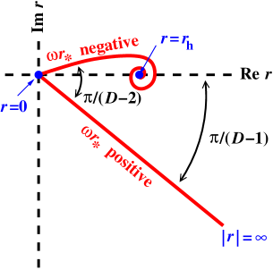
Figure 2: A qualitative picture of the relevant Stokes lines $\operatorname{Im}(\omega r_{*})=0$ in the complex $r$ plane for following WKB between the boundary ($r=\infty$) and the horizon ($r=r_{\rm h}$). The path passes through the singularity ($r=0$) in SAdS_D. The other Stokes lines emanating from the origin are not shown, one of which escapes to $-e^{-i\pi/(D-1)}\infty$ and the others which spiral into the complex-valued horizons $r=e^{-i2n\pi/(D-1)}r_{\rm h}$ for $n=1,\cdots,D-2$. (The spiral into the horizon shown above crosses a cut in the definition of $r_{*}$ emanating from $r=r_{\rm h}$, and the curve spirals onto higher and higher Riemann sheets.) Given our retarded convention for $\omega$, this figure is the complex conjugate of similar diagrams in refs. NatarioSchiappa ; CardosoNatarioSchiappa .

Given our conventions, the tortoise coordinate $r_{*}$ vanishes at the singularity $r{=}0$, the Stokes line from the singularity to $|r|{=}\infty$ has $\omega r_{*}$ positive, and the Stokes line from the singularity to the horizon $r{=}r_{\rm h}$ has $\omega r_{*}$ negative.

Note, by the way, that (29) is the form of the exact solution to the Dirac equation (27) in the case that both $m$ and ${\bm{k}}$ are zero. However, (29) cannot simultaneously satisfy the quasinormal mode boundary conditions that it vanish at the boundary of AdS and that it have only the $e^{-i\omega r_{*}}$ component at the horizon. The existence of any quasinormal mode solution therefore depends on non-zero $m$ or ${\bm{k}}$. This will be the origin of why our asymptotic formula (6) for $\omega_{n}$ depends on $|{\bm{k}}|$.

II.3 Matching at the boundary $r\to\infty$

Near the boundary, $f\to 1$ and the SAdS metric approaches that of pure AdS. The Dirac equation (27) reduces to

$$\left[\frac{r^{2}}{L^{2}}\,\partial_{r}-i\omega\tau_{2}+\frac{mr}{L}\,\tau_{3}+k\tau_{1}\right]\begin{pmatrix}\psi_{+}\\ \psi_{-}\end{pmatrix}\simeq 0$$ (32)

or equivalently

$$\left[\partial_{z}+i\omega\tau_{2}-\frac{mL}{z}\,\tau_{3}-k\tau_{1}\right]\begin{pmatrix}\psi_{+}\\ \psi_{-}\end{pmatrix}\simeq 0,$$ (33)

whose solution is well known Henningson ; Leigh . Applying $-\partial_{z}+i\omega\tau_{2}-mLz^{-1}\tau_{3}-k\tau_{1}$ to (33),

$$\left[-\partial_{z}^{2}+\frac{(2mL-1)^{2}-1}{4z^{2}}\right]\psi_{+}=\Omega^{2}\psi_{+},$$ (34)

$$\left[-\partial_{z}^{2}+\frac{(2mL+1)^{2}-1}{4z^{2}}\right]\psi_{-}=\Omega^{2}\psi_{-},$$ (35)

where

$$\Omega^{2}\equiv\omega^{2}-|{\bm{k}}|^{2}.$$ (36)

Independent solutions may be expressed in terms of Bessel functions as $\sqrt{\Omega z}\,J_{\nu}(\Omega z)$ and $\sqrt{\Omega z}\,Y_{\nu}(\Omega z)$ with $\nu=mL\mp\tfrac{1}{2}$ for $\psi_{\pm}$. Note that solutions for $\psi_{+}$ and $\psi_{-}$ are not independent from each other but are related by the original equation (33).

II.3.1 Massive fields

For massive fields, we may impose the boundary condition that the field $\psi$ vanish at the boundary $z{=}0$, which selects the $J_{\nu}$ solutions. The corresponding solution to the original first-order equation (33) is

$$\begin{pmatrix}\psi_{+}\\ \psi_{-}\end{pmatrix}\propto\begin{pmatrix}\sqrt{2\pi\Omega z}\,J_{mL-\frac{1}{2}}(\Omega z)\\ \frac{\Omega}{\omega-k}\,\sqrt{2\pi\Omega z}\,J_{mL+\frac{1}{2}}(\Omega z)\end{pmatrix}.$$ (37)

We’re interested in the large-$\omega$ limit of $|\omega|\gg|{\bm{k}}|$, in which case this becomes

$$\begin{pmatrix}\psi_{+}\\ \psi_{-}\end{pmatrix}\propto\begin{pmatrix}\sqrt{2\pi\omega z}\,J_{mL-\frac{1}{2}}(\omega z)\\ \sqrt{2\pi\omega z}\,J_{mL+\frac{1}{2}}(\omega z)\end{pmatrix}$$ (38)

with asymptotic expansion

$$\begin{pmatrix}\psi_{+}\\ \psi_{-}\end{pmatrix}\propto\begin{pmatrix}2\cos(\omega z-\tfrac{\pi}{2}\,mL)\\ 2\sin(\omega z-\tfrac{\pi}{2}\,mL)\end{pmatrix}=\begin{pmatrix}e^{-imL\pi/2}e^{i\omega z}+e^{imL\pi/2}e^{-i\omega z}\\ -ie^{-imL\pi/2}e^{i\omega z}+ie^{imL\pi/2}e^{-i\omega z}\end{pmatrix}$$ (39)

away from the boundary (i.e. for $\omega z\gg 1$). It will be useful later to rewrite this in terms of $\tau_{1}$ as

$$\begin{pmatrix}\psi_{+}\\ \psi_{-}\end{pmatrix}\propto\left[-i\tau_{1}e^{-imL\pi/2}e^{i\omega z}+e^{imL\pi/2}e^{-i\omega z}\right]\begin{pmatrix}1\\ i\end{pmatrix}.$$ (40)

In order to move beyond the $z{\ll}z_{\rm h}$ approximation, we need to match the asymptotic form (40) to the general WKB form (29). To that end, we need the near-boundary expression for the tortoise coordinate $r_{*}$ of (31), which is

$$r_{*}\simeq r_{*0}-z,$$ (41)

where, for the $f$ specific to SAdS (5),

$$r_{*0}\equiv r_{*}\bigr{|}_{\rm boundary}=\frac{\pi e^{i\pi/(D-1)}}{F^{\prime}(r_{\rm h})\sin(\frac{\pi}{D-1})}=\frac{e^{i\pi/(D-1)}}{4T\sin(\frac{\pi}{D-1})}.$$ (42)

And so (40) may be written as

$$\psi\propto\left[e^{imL\pi/2}e^{-i\omega r_{*0}}e^{i\omega r_{*}}-i\tau_{1}e^{-imL\pi/2}e^{i\omega r_{*0}}e^{-i\omega r_{*}}\right]\begin{pmatrix}1\\ i\end{pmatrix}.$$ (43)

It will be useful later to imagine expanding the result in terms of $\tau_{1}$ eigenstates. We won’t actually need to be any more explicit than we already have been, but one could accordingly rewrite

$$\begin{pmatrix}1\\ i\end{pmatrix}\propto e^{i\pi/4}\begin{pmatrix}1\\ 1\end{pmatrix}+e^{-i\pi/4}\begin{pmatrix}1\\ -1\end{pmatrix}$$ (44)

above, if desired.

II.3.2 Massless fields

For the massless case $m{=}0$, the solutions involving $J_{\nu}$ and $Y_{\nu}$ near the boundary are

$$\begin{pmatrix}\psi_{+}\\ \psi_{-}\end{pmatrix}\propto\begin{pmatrix}\cos(\Omega z)\\ \frac{\Omega\sin(\Omega z)}{\omega-k}\end{pmatrix}$$ (45)

and

$$\begin{pmatrix}\psi_{+}\\ \psi_{-}\end{pmatrix}\propto\begin{pmatrix}\sin(\Omega z)\\ -\frac{\Omega\cos(\Omega z)}{\omega-k}\end{pmatrix}$$ (46)

respectively, and no non-trivial combination vanishes at the boundary. Our interest in this case will be for comparison with the numerical results of Giammatteo and Jing GiammatteoJing , and so we should apply their boundary conditions, which in our language is that $\psi_{+}=\psi_{-}$ at the boundary. In the large $\omega$ limit of interest, this fixes the combination to be

$$\begin{pmatrix}\psi_{+}\\ \psi_{-}\end{pmatrix}\propto\begin{pmatrix}\cos(\omega z)-\sin(\omega z)\\ \sin(\omega z)+\cos(\omega z)\end{pmatrix},$$ (47)

which can be rewritten as

$$\begin{pmatrix}\psi_{+}\\ \psi_{-}\end{pmatrix}\propto e^{-i\pi/4}\left[\tau_{1}e^{i\omega z}+e^{-i\omega z}\right]\begin{pmatrix}1\\ i\end{pmatrix}\simeq e^{-i\pi/4}\left[e^{-i\omega r_{*0}}e^{i\omega r_{*}}+\tau_{1}e^{i\omega r_{*0}}e^{-i\omega r_{*}}\right]\begin{pmatrix}1\\ i\end{pmatrix}.$$ (48)

This $m{=}0$ case with Giammatteo’s and Jing’s boundary condition has the same asymptotic expansion as the $mL=\tfrac{3}{2}$ case of (43), which implemented the usual boundary condition of avoiding singularities at the boundary for $m>0$. As it turns out, the matching near the boundary is the only place where the mass $m$ will enter the calculation of the quasi-normal mode frequencies to the order at which we are working. So we need not discuss the massless case any further: to compare to Giammatteo and Jing, just set $D=4$ and $mL=\tfrac{3}{2}$ in the formulas that we will derive for the massive case.

II.4 Matching at $r\to 0$

From the previous discussion, we now know the asymptotic expansion along the Stokes line from $|r|=\infty$ to the singularity $r=0$ in fig. 2. For now, let’s generically refer to this expansion as

$$\phi\simeq{\cal B}_{+}e^{i\omega r_{*}}+{\cal B}_{-}e^{-i\omega r_{*}}\qquad\mbox{($\omega r_{*}$ positive)},$$ (49)

and we will save for later using the explicit from (43). Our task now is to solve the Dirac equation near the singularity and thereby relate the coefficients ${\cal B}_{\pm}$ above to coefficients ${\cal A}_{\pm}$ for a similar asymptotic expansion along the other Stokes line in fig. 2, which leads to the horizon:

$$\phi\simeq{\cal A}_{+}e^{i\omega r_{*}}+{\cal A}_{-}e^{-i\omega r_{*}}\qquad\mbox{($\omega r_{*}$ negative)}.$$ (50)

II.4.1 The $r\to 0$ Schrödinger problem

For small $r$ and large $\omega$, the dominant terms in the Dirac equation (27) are

$$\left[F\partial_{r}-i\omega\tau_{2}-ik\left(\frac{r_{\rm h}}{r}\right)^{(D-1)/2}\tau_{1}\right]\begin{pmatrix}\psi_{+}\\ \psi_{-}\end{pmatrix}\simeq 0,$$ (51)

assuming ${\bm{k}}\not=0$. Now apply $-F\partial_{r}-i\omega\tau_{2}-ik(r_{\rm h}/r)^{(D-1)/2}\tau_{1}$ to (51), and expand. The result is a Schrödinger-like equation

$$\left[-\partial_{r_{*}}^{2}+V_{\rm sing}(r)\right]\psi\simeq\omega^{2}\psi,$$ (52)

with

$$V_{\rm sing}(r)=-k^{2}\left(\frac{r_{\rm h}}{r}\right)^{D-1}+i\tau_{1}k\,\frac{(D-1)r_{\rm h}^{3(D-1)/2}}{2L^{2}\,r^{(3D-5)/2}}.$$ (53)

For the case of $D>3$ considered in this paper, the first term in (54) is sub-dominant for small $r$ and so may be dropped:

$$V_{\rm sing}(r)\simeq+i\tau_{1}k\,\frac{(D-1)r_{\rm h}^{3(D-1)/2}}{2L^{2}\,r^{(3D-5)/2}}.$$ (54)

Now rewrite this potential in terms of the tortoise coordinate $r_{*}$. For small $r$, (25) and/or (31) give

$$r_{*}=\int_{0}^{r}\frac{dr^{\prime}}{F(r^{\prime})}\simeq-\frac{L^{2}r^{D-2}}{(D-2)r_{\rm h}^{D-1}},$$ (55)

and so

$$r\simeq e^{-i\pi/(D-2)}\left[\frac{(D-2)r_{\rm h}^{D-1}r_{*}}{L^{2}}\right]^{1/(D-2)}\,.$$ (56)

Then

$$V_{\rm sing}\simeq-\tau_{1}\frac{\kappa}{r_{*}^{2-a}}$$ (57)

with $a$ defined as in (9) and

$$\kappa\equiv e^{i\pi(\frac{3}{2}-a)}\,\frac{(D-1)}{2(D-2)^{2-a}}\left(\frac{L^{2}}{r_{\rm h}}\right)^{1-a}k.$$ (58)

II.4.2 The solution

We want to solve the equation

$$\left[-\partial_{r_{*}}^{2}-\tau_{1}\,\frac{\kappa}{r_{*}^{2-a}}\right]\psi=\omega^{2}\psi.$$ (59)

It’s convenient to think in terms of eigenstates of $\tau_{1}$ and treat $\tau_{1}$ simply as a sign $\pm$ in what follows. Accordingly, defining the number $\bar{\kappa}\equiv\tau_{1}\kappa$ and dropping consideration of the spinor structure, our equation has the form

$$\left[-\partial_{r_{*}}^{2}-\frac{\bar{\kappa}}{r_{*}^{2-a}}\right]\phi=\omega^{2}\phi.$$ (60)

We don’t know of a closed form solution to this equation. However, in the large $\omega$ limit, we can see that it is adequate to solve perturbatively in $\bar{\kappa}$. Treating $\bar{\kappa}/r_{*}^{2-a}$ as small compared to $\omega^{2}$ requires

$$|r_{*}|\gg\left|\frac{\bar{\kappa}}{\omega^{2}}\right|^{1/(2-a)}.$$ (61)

On the other hand, in order to match the WKB expansions (49) to (50), we need the solution in a region where neither $e^{+i\omega r_{*}}$ nor $e^{-i\omega r_{*}}$ becomes exponentially small (and so small compared to the approximation error in the other solution) at any time in the process of rotating $\arg(\omega r_{*})$ from $0$ to $\pi$. That requires

$$|\omega r_{*}|\lesssim 1.$$ (62)

Fortunately, both conditions (61) and (62) can be simultaneously satisfied if

$$|\bar{\kappa}|\ll|\omega|^{a}.$$ (63)

Since $a=(D-3)/2(D-2)$, (63) will always be satisfied for sufficiently large $|\omega|$ at fixed $|{\bm{k}}|$ provided that $D>3$. Using (7) and (58), the condition can be cast into the form

$$\frac{|{\bm{k}}|}{T}\ll\left(\frac{|\omega|}{T}\right)^{2-a}.$$ (64)

The solutions to the unperturbed ($\bar{\kappa}{=}0$) version of (60) are simply $e^{\pm i\omega r_{*}}$. So write $\phi=e^{\pm i\omega r_{*}}(1+\bar{\kappa}\xi)$ and linearize the equation in $\bar{\kappa}$, giving

$$e^{\mp 2i\omega r_{*}}\partial_{r_{*}}\left(e^{\pm 2i\omega r_{*}}\partial_{r_{*}}\xi\right)\simeq-\frac{1}{r_{*}^{2-a}}\,.$$ (65)

The corresponding solutions are

$$\phi^{(\pm)}\simeq e^{\pm i\omega r_{*}}\left[1-\bar{\kappa}\int_{r_{*}}^{\infty}dr_{*}^{\prime}\>e^{\mp 2i\omega r_{*}^{\prime}}\int_{r_{*}^{\prime}}^{\infty}dr_{*}^{\prime\prime}\>\frac{e^{\pm 2i\omega r_{*}^{\prime\prime}}}{(r_{*}^{\prime\prime})^{2-a}}\right].$$ (66)

The integral gives

$$\phi^{(\pm)}\simeq e^{\pm i\omega r_{*}}+\bar{\kappa}\,\frac{\Gamma(a,\mp 2i\omega r_{*})}{(\mp 2i\omega)^{a}(1-a)}\,e^{\mp i\omega r_{*}},$$ (67)

where $\Gamma(a,z)$ is the incomplete $\Gamma$ function

$$\Gamma(a,z)\equiv\int_{z}^{\infty}dt\>e^{-t}t^{a-1}\equiv\Gamma(a)-\gamma(a,z).$$ (68)

II.4.3 The matching

The asymptotic behavior of the incomplete $\Gamma$ function is

$$\Gamma(a,z)\simeq z^{a-1}e^{-z}\qquad\mbox{($|z|\to\infty$ with $|\arg z|<\frac{3\pi}{2}$)}.$$ (69)

For positive real $\omega r_{*}$, the magnitude of the second term in the solution (67) therefore falls algebraically for $\omega r_{*}\gg 1$ since the exponent $a-1=-(D-1)/2(D-2)$ is negative, and so the asymptotic behavior of these solutions is

$$\phi^{(\pm)}\to e^{\pm i\omega r_{*}}\qquad\mbox{($\omega r_{*}$ positive)}.$$ (70)

We now need to match this to the asymptotic behavior on the negative $\omega r_{*}$ Stokes line in fig. 2. Near the origin, moving from the positive $\omega r_{*}$ line clockwise to the negative $\omega r_{*}$ line in that figure corresponds to rotating $r$ by $e^{i\pi/(D-2)}$ and $r_{*}$ by $e^{i\pi}$. Then, along the negative $\omega r_{*}$ Stokes line, $\arg(-i\omega r_{*})=\frac{\pi}{2}$ again satisfies the condition for (69), and so

$$\phi^{(+)}\to e^{i\omega r_{*}}\qquad\mbox{($\omega r_{*}$ negative)}$$ (71)

just like in (70).

The interesting case is what happens to the asymptotic expansion of $\phi^{(-)}$ when we analytically continue from the positive $\omega r_{*}$ line to the negative $\omega r_{*}$ line. In order to keep phases straight, it is convenient to rewrite

$$\omega r_{*}=e^{i\pi}\omega y$$ (72)

along the negative $\omega r_{*}$ Stokes line, with $\omega y=-\omega r_{*}$ positive. In this case, $\arg(i\omega r_{*})=\frac{3\pi}{2}$, which does not satisfy the condition of (69). From the integral formula

$$\gamma(a,z)\equiv\int_{0}^{z}dt\>e^{-t}t^{a-1},$$ (73)

one can show the monodromy relation

$$\gamma(a,e^{i2\pi n}z)=e^{i2\pi na}\gamma(a,z)$$ (74)

for integer $n$, and so

$$\Gamma(a,e^{i2\pi n}z)=[1-e^{i2\pi na}]\Gamma(a)+e^{i2\pi na}\Gamma(a,z).$$ (75)

Using this relation, we can rewrite

$$\Gamma(a,2i\omega r_{*})=\Gamma(a,e^{i3\pi/2}2\omega y)=[1-e^{i2\pi a}]\Gamma(a)+e^{i2\pi a}\,\Gamma(a,e^{-i\pi/2}2\omega y)$$ (76)

and then use the standard expansion (69) to show that the last term disappears at large positive $\omega y$. The result is that (67) yields

$$\phi^{(-)}\to e^{-i\omega r_{*}}-\bar{\kappa}\,\frac{[1-e^{i2\pi a}]\,\Gamma(a)}{(2e^{i\pi/2}\omega)^{a}(1-a)}\,e^{i\omega r_{*}}\qquad\mbox{($\omega r_{*}$ negative)}.$$ (77)

Using $\bar{\kappa}\equiv\tau_{1}\kappa$ and (58) for $\kappa$ and (7) for $T$, this can be written as

$$\phi^{(-)}\to e^{-i\omega r_{*}}+\tau_{1}\lambda\,\frac{(k/\pi T)}{(\omega/\pi T)^{a}}\,e^{i\omega r_{*}}\qquad\mbox{($\omega r_{*}$ negative)},$$ (78)

where

$$\lambda\equiv e^{-i\pi a/2}(1-a)^{1-a}\,\Gamma(a)\sin(\pi a).$$ (79)

The upshot of (70), (71), and (78) is that an expansion

$$\phi\simeq{\cal B}_{+}e^{i\omega r_{*}}+{\cal B}_{-}e^{-i\omega r_{*}}$$ (80)

on the positive $\omega r_{*}$ Stokes line corresponds to an expansion

$$\phi\simeq\left[{\cal B}_{+}+\tau_{1}\lambda\,\frac{(k/\pi T)}{(\omega/\pi T)^{a}}\,{\cal B}_{-}\right]e^{i\omega r_{*}}+{\cal B}_{-}e^{-i\omega r_{*}}$$ (81)

on the negative $\omega r_{*}$ Stokes line. Writing the latter as

$$\phi\simeq{\cal A}_{+}e^{i\omega r_{*}}+{\cal A}_{-}e^{-i\omega r_{*}}\qquad\mbox{($\omega r_{*}$ negative)},$$ (82)

the relationship is

$$\begin{pmatrix}{\cal A}_{+}\\ {\cal A}_{-}\end{pmatrix}=\begin{pmatrix}1&\tau_{1}\lambda\,\frac{(k/\pi T)}{(\omega/\pi T)^{a}}\\ 0&1\end{pmatrix}\begin{pmatrix}{\cal B}_{+}\\ {\cal B}_{-}\end{pmatrix}.$$ (83)

II.5 Putting it all together

We now impose the infalling boundary condition at the horizon, which is that the $e^{i\omega r_{*}}$ term in the expansion (82) must vanish along the negative $\omega r_{*}$ Stokes line that connects the singularity $r{=}0$ to the horizon. From (81) that condition is

$${\cal B}_{+}=-\tau_{1}\lambda\,\frac{(k/\pi T)}{(\omega/\pi T)^{a}}\,{\cal B}_{-}.$$ (84)

On the other hand, along the positive $\omega r_{*}$ Stokes line, comparison of the WKB form (49) to the form (43) that we got from applying the quasinormal mode condition at the boundary ($r\to\infty$) gives

$${\cal B}_{-}=-i\tau_{1}e^{2i\omega r_{*0}-imL\pi}{\cal B}_{+}.$$ (85)

Consistency of (84) and (85) requires the condition

$$i\lambda\,\frac{(k/\pi T)}{(\omega/\pi T)^{a}}\,e^{2i\omega r_{*0}-imL\pi}=1,$$ (86)

which determines the quasi-normal mode frequencies. This condition is satisfied when

$$i\tfrac{\pi}{2}+\ln\left(\lambda\,\frac{(k/\pi T)}{(\omega/\pi T)^{a}}\right)+2i\omega r_{*0}-imL\pi=i2\pi n$$ (87)

for integer $n$. Solving for $\omega$ by iteration in the large $n$ limit, and using eq. (42) for $r_{*0}$ and (79) for $\lambda$, then produces the result

$$\frac{\omega_{n\pm}}{\pi T}\simeq 4e^{-i\pi/(D-1)}\sin\Bigl{(}\frac{\pi}{D-1}\Bigr{)}\\ \times\left[n-\frac{i}{2\pi}\ln\left(\frac{n^{a}}{k/\pi T}\right)+\tfrac{1}{2}(|mL|-\tfrac{1}{2})+\frac{(D-3)^{2}}{8(D-1)(D-2)}+\frac{i\xi}{\pi}\right],$$ (88)

with $\xi$ defined as in (8). Now recall from the definition (26) of $k$ that $k=\pm|{\bm{k}}|$, depending on the spin state. Eq. (88) may then be recast in terms of $|{\bm{k}}|$ as the result (6) quoted in the introduction.

III Numerical Method

In this section, we discuss our numerical method for finding quasinormal mode frequencies in the massive case, which we will use to test the asymptotic result (6). We have not made exhaustive comparisons to find the most efficient numerical algorithm in the spin-$1/2$ case, but we will just use a variation on one of the methods often used in the literature. We will find a recursion relation for a series solution to the Dirac equation expanded about the horizon. We will use that recursion relation to evaluate that series at the AdS boundary as a function of $\omega$ (for given $m$ and $|{\bm{k}}|$). Then we will search the complex $\omega$ plane to find values $\omega{=}\omega_{n}$ where the value at the AdS boundary vanishes.

It is useful to have an equation that eliminates the spinor structure from the Dirac equation (27). It is also convenient to have an equation that does not involve square roots of $f$, since square roots in our equation will not generate a recursion relation (for the series solution) that has a bounded number of terms. (However, if one must, it is possible to get by with an unbounded number of terms in the recursion relation, as in ref. GiammatteoJing ).

To obtain the equation we will use, start with the Dirac equation (27) and change basis to rewrite it in terms of

$$A\equiv\frac{\psi_{+}+i\psi_{-}}{\sqrt{2}},\qquad B\equiv\frac{i\psi_{+}+\psi_{-}}{\sqrt{2}},$$ (89)

to get

$$\left[F\partial_{r}+i\omega\tau_{3}+mF^{1/2}\tau_{2}+f^{1/2}k\tau_{1}\right]\begin{pmatrix}A\\ B\end{pmatrix}=0.$$ (90)

In terms of components,

$$(F\partial_{r}+i\omega)A =-\Bigl{(}k-\frac{imr}{L}\Bigr{)}f^{1/2}B,$$ (91)

$$(F\partial_{r}-i\omega)B =-\Bigl{(}k+\frac{imr}{L}\Bigr{)}f^{1/2}A.$$ (92)

Rewrite the last as

$$f^{-1/2}(F\partial_{r}-i\omega)f^{-1/2}f^{1/2}B=-\Bigl{(}k+\frac{imr}{L}\Bigr{)}A.$$ (93)

Combining (91) and (93),

$$f^{-1/2}(F\partial_{r}-i\omega)\left[f^{-1/2}\Bigl{(}k-\frac{imr}{L}\Bigr{)}^{-1}(F\partial_{r}+i\omega)A\right]=\Bigl{(}k+\frac{imr}{L}\Bigr{)}A,$$ (94)

which may be expanded to

$$(F\partial_{r})^{2}A+\left(-\frac{r^{2}\partial_{r}f}{2L^{2}}+\frac{imF}{kL-imr}\right)(F\partial_{r}+i\omega)A+(\omega^{2}-m^{2}F-k^{2}f)A=0.$$ (95)

This equation does not involve any square roots of $f$. By multiplying through by $kL-imr$, it will be possible to write an equation whose power-series solutions will have recursion relations with a fixed number of terms.

We note in passing that the massless version of (95) is related to the Teukolsky equation which is often used to simultaneously study massless fields of all different spins in $D{=}4$. We point out the translation to a selection of formulas in the literature in appendix A.

Now factor out the behavior of the solution near the horizon and near the boundary by writing

$$A(z)=z^{-mL}e^{-i\omega r_{*}}H(z),$$ (96)

where $z=L^{2}/r$. The equation for $H$ is then

$$zf\partial_{z}^{2}H+\left(2i\omega z-2\bar{m}f+\frac{z\partial_{z}f}{2}-\frac{i\bar{m}f}{kz-i\bar{m}}\right)\partial_{z}H\\ -\left[\bar{m}^{2}\,\frac{(1-f)}{z}+\bar{m}\left(2i\omega+\frac{\partial_{z}f}{2}-\frac{kf}{kz-i\bar{m}}\right)+k^{2}z\right]H=0,$$ (97)

where we have introduced the dimensionless mass

$$\bar{m}\equiv mL.$$ (98)

Multiplying through by $kz-i\bar{m}$, and specializing now to units where $z_{\rm h}=1$, one can obtain a recursion relation for a series solution

$$H(z)=\sum_{n=0}^{\infty}a_{n}(1-z)^{n}$$ (99)

about the horizon. For $D{=}5$, this is a 6-term recursion relation for the coefficients $a_{n}$, which is the shortest recursion relation we were able to find for the massive case. Specifically, for $D{=}5$, the choice of units $z_{\rm h}=1$ is $\pi T=1$ and the recursion relation is

$$\sum_{j=0}^{5}\alpha_{-j}(n)\,a_{n-j}=0$$ (100)

with

$$\alpha_{-5} =-(4+\bar{m}-n)(5+\bar{m}-n)k,$$ (101)

$$\alpha_{-4} =(4+\bar{m}-n)\bigl{[}(20+4\bar{m}-6n)k+(-2-\bar{m}+n)i\bar{m}\bigr{]},$$ (102)

$$\alpha_{-3} =(-120-54\bar{m}-6\bar{m}^{2}+85n+20\bar{m}n-15n^{2})k-k^{3}$$

$$\qquad+(24+18\bar{m}+3\bar{m}^{2}-23n-8\bar{m}n+5n^{2})i\bar{m},$$ (103)

$$\alpha_{-2} =(80+36\bar{m}+4\bar{m}^{2}-80n-20\bar{m}n+20n^{2})k+2k^{3}$$

$$\qquad+(-24-18\bar{m}-3\bar{m}^{2}+32n+12\bar{m}n-10n^{2})i\bar{m}-ik^{2}\bar{m}+(4+2\bar{m}-2n)ik\omega,$$ (104)

$$\alpha_{-1} =(-18-6\bar{m}-\bar{m}^{2}+32n+8\bar{m}n-14n^{2})k-k^{3}$$

$$\qquad+(8+6\bar{m}+\bar{m}^{2}-18n-8\bar{m}n+10n^{2})i\bar{m}$$

$$\qquad+ik^{2}\bar{m}+(-2-2\bar{m}+2n)\bar{m}\omega+(-4-2\bar{m}+4n)ik\omega,$$ (105)

$$\alpha_{0} =2n(k-i\bar{m})(-1+2n-i\omega).$$ (106)

Our numerical method is to use this recursion relation to calculate all the $a_{n}$ while computing the value of $H$ at the boundary as

$$H(z{=}0)=\sum_{n=0}^{\infty}a_{n}$$ (107)

(cut off at some suitably high value of $n$), and then to scan the complex $\omega$ plane to find zeros of (107).

IV Numerics compared to asymptotic formula

IV.1 Massive $D{=}5$

We have already shown in fig. 1 one comparison of our $D{=}5$ numerical results for $\omega_{n}$ with the asymptotic formula (10) In order to check more accurately, it is helpful to study much higher $n$ and to plot the offset $\delta_{n}$ from the leading $O(n)$ asymptotic formula, defined by

$$\delta_{n}\equiv\frac{\omega_{n}}{\Delta\omega_{\infty}}-n\equiv\frac{\omega_{n}}{2(1-i)\pi T}-n$$ (108)

(for $D{=}5$). Fig. 3 shows data points for $\delta_{n+}$ from numerics plotted against dashed lines showing the asymptotic result taken from (10):

$$\frac{\omega_{n\pm}}{\pi T}\simeq 2(1-i)\left[n-\frac{i}{2\pi}\ln\left(\frac{n^{1/3}}{|{\bm{k}}|/\pi T}\right)+\tfrac{1}{2}(|mL|-1\pm\tfrac{1}{2})+\frac{1}{24}+\frac{i\xi_{5}}{\pi}\right].$$ (109)

In particular, the large $n$ behavior of $\operatorname{Im}\delta_{n+}$ in fig. 3b clearly shows agreement with the asymptotic $\log n$ and $|{\bm{k}}|$ dependence found in (109).

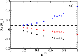
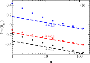
Figure 3: A plot of the (a) real and (b) imaginary parts of the offsets $\delta_{n}$ defined by (108) for $D=5$, $mL=\tfrac{1}{2}$, $|{\bm{k}}|/\pi T=0.1$, $0.3$, and $2.3$, and the representative overtones $n=1,2,4,8,16,\cdots,128$. Data points are from our numerics, whereas the dashed lines indicate the value of $\delta_{n}$ that would be given by the asymptotic formula (109). Note the different choices made for the horizontal axis in the two figures, and that large $n$ corresponds to the left and right hand sides of (a) and (b) respectively.

For the sake of comparison for anyone in the future making similar calculations, we provide tables of some of our numerical results in appendix B.

IV.2 Massless $D{=}4$

For the case of massless fermions in $D{=}4$, fig. 4 shows a comparison of our asymptotic formula (12) with numerical results of Giammatteo and Jing GiammatteoJing . In order to facilitate comparison, it is useful to use (7) to recast (12) as

$$\frac{\omega L^{2}}{r_{\rm h}}\simeq e^{-i\pi/3}\frac{3^{3/2}}{2}\left[n-\frac{i}{2\pi}\ln\left(\frac{n^{1/4}}{4|{\bm{k}}|L^{2}/3r_{\rm h}}\right)+\frac{25}{48}+\frac{i\xi_{4}}{\pi}\right].$$ (110)

Giammatteo and Jing study different sizes of black holes, whereas our asymptotic formula was only derived in the large black hole limit, and so we compare only to their results for their largest black hole. Their $r_{1}$ is our $r_{\rm h}/L$, and their largest black holes correspond to Table II of ref. GiammatteoJing with $r_{1}=100$. Their $k$ is an integer, related to the mode of spherical harmonics, but translates in the large black hole limit into our $|{\bm{k}}|L$. In their Table II, the columns labeled $\ell=0$ and $\ell=1$ correspond to their $k=1$ and $k=2$ respectively. Their dimensionless $\omega$ quoted in numerical results is simply our $\omega L$. That is, they work in units where $L=1$.

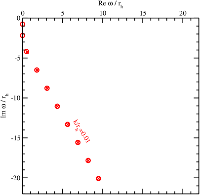
Figure 4: Retarded quasi-normal mode frequencies in the lower-right quadrant of the complex $\omega$ plane for massless $D{=}4$ Dirac fermions. The red circles are numerical results taken from the $\ell{=}0$ column of Table II of ref. GiammatteoJing and corresponds to $|{\bm{k}}|=0.01\,r_{\rm h}$. The crosses show the asymptotic formula (110) for $\omega_{n+}$. (We do not also show the $\ell=1$ results here because they would crowd too close to the $\ell=0$ results.)

As in the earlier discussion of $D{=}5$, we also look at the offset $\delta_{n}$, which in the $D{=}4$ case is

$$\delta_{n}\equiv\frac{\omega_{n}}{\Delta\omega_{\infty}}-n\equiv\frac{\omega_{n}}{(\frac{3\sqrt{3}}{4}-\frac{9i}{4})r_{\rm h}}-n.$$ (111)

Fig. 5 shows data points for $\delta_{n+}$ from Giammatteo and Jing plotted against dashed lines showing the asymptotic result taken from (110). The agreement at large $n$ (and even small $n$) is quite good.

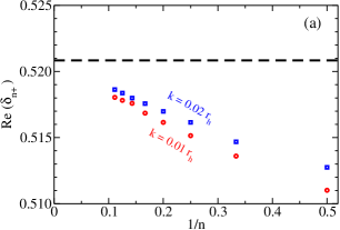
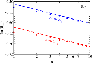
Figure 5: The (a) real and (b) imaginary parts of the offsets $\delta_{n}$ defined by (111) extracted from the $\ell=0$ and $\ell=1$ numerical results (corresponding to $|{\bm{k}}|=0.01\,r_{\rm h}$ and $0.02\,r_{\rm h}$ respectively) of Table II of ref. GiammatteoJing for massless Dirac fermions in $D{=}4$. The dashed lines indicate the value of $\delta_{n}$ that would be given by the asymptotic formula (110). In order to align the overtones found in ref. GiammatteoJing with the ones given by our asymptotic formula, the overtone number $n$ we use in this figure corresponds to their $n-1$.

Appendix A Relation to Teukolsky equation

In this appendix, it will be convenient to set $L{=}1$. In the massless case, the form (95) of the Dirac equation becomes

$$(F\partial_{r})^{2}A-\frac{r^{2}\partial_{r}f}{2}(F\partial_{r}+i\omega)A+(\omega^{2}-k^{2}f)A=0,$$ (112)

If one now defines $\psi_{1/2}$ by

$$A=f^{1/4}\psi_{1/2},$$ (113)

then the equation becomes the Schrödinger-like problem

$$\left[-\partial_{r_{*}}^{2}+V_{1/2}\right]\psi_{1/2}=\omega^{2}\psi_{1/2}$$ (114a)

with

$$V_{1/2}(r)=-\tfrac{1}{4}\,F\partial_{r}(r^{2}f^{\prime})+\tfrac{1}{16}\,r^{4}(f^{\prime})^{2}+\tfrac{1}{2}\,i\omega r^{2}f^{\prime}+k^{2}f.$$ (114b)

Though the above equations are valid in any dimension, they agree with the spin-$\tfrac{1}{2}$ case of the Teukolsky equation Teukolsky . The Teukolsky equation gives a unified description of arbitrary-spin massless fields in certain $D{=}4$ metrics, and has been used by a number of authors to study quasinormal modes for asymptotically flat Schwarzschild and Kerr-Newman. Our eqs. (114) are equivalent, for example, to the particular form of the Teukolsky equation given by Jing Jing . For more specific comparison to papers on asymptotically flat $D{=}4$ Schwarzschild black holes, note that the metric (3b) has the same form as an asymptotically flat $D{=}4$ black hole metric if one identifies

$$F=1-\frac{r_{\rm h}}{r}\,,\qquad f\equiv\frac{F}{r^{2}}\,,$$ (115)

and takes ${\bm{x}}$ to be angular variables approximated as flat (an approximation that will make sense in the limit of large spherical harmonics).

For discussion of the Teukolsky equation in asymptotically AdS₄ spacetime, see ref. GiammatteoMoss . We our unaware of any generalization of the Teukolsky equation for arbitrary spin to $D>4$.

Appendix B Tabulated numerical results for exact quasinormal frequencies

For the sake of anyone who might want to someday compare their own numerics to our results, we tabulate some quasinormal mode frequencies in table 1.

$n\pm$	$\omega_{n\pm}/\pi T$
	$|{\bm{k}}|=0.1\,\pi T$		$|{\bm{k}}|=0.3\,\pi T$		$|{\bm{k}}|=2.3\,\pi T$
1$-$	1.09696	-1.80921 $i$	1.10987	-1.49754 $i$	2.75050	-0.76673 $i$
1$+$	1.37370	-2.09426 $i$	1.69167	-2.10603 $i$	3.36431	-1.61242 $i$
2$-$	2.91046	-3.98067 $i$	2.91651	-3.60052 $i$	4.18969	-2.70882 $i$
2$+$	3.29582	-4.28446 $i$	3.63039	-4.24441 $i$	5.01324	-3.65993 $i$
3$-$	4.80706	-6.05121 $i$	4.83157	-5.64176 $i$	5.93557	-4.75183 $i$
3$+$	5.24680	-6.38134 $i$	5.59180	-6.31677 $i$	6.82779	-5.71511 $i$
4$-$	6.73512	-8.09412 $i$	6.77754	-7.66773 $i$	7.78860	-6.79412 $i$
4$+$	7.21246	-8.44691 $i$	7.56440	-8.36564 $i$	8.71124	-7.76006 $i$
5$-$	8.68030	-10.12411 $i$	8.73829	-9.68687 $i$	9.69036	-8.82896 $i$
5$+$	9.18625	-10.49627 $i$	9.54318	-10.40232 $i$	10.62949	-9.79610 $i$
6$-$	10.63622	-12.14674 $i$	10.70765	-11.70209 $i$	11.61867	-10.85756 $i$
6$+$	11.16516	-12.53573 $i$	11.52585	-12.43157 $i$	12.56796	-11.82560 $i$
7$-$	12.59951	-14.16467 $i$	12.68262	-13.71478 $i$	13.56322	-12.88148 $i$
7$+$	13.14755	-14.56851 $i$	13.51120	-14.45582 $i$	14.51937	-13.85031 $i$
8$-$	14.56816	-16.17939 $i$	14.66151	-15.72568 $i$	15.51857	-14.90188 $i$
8$+$	15.13247	-16.59648 $i$	15.49851	-16.47650 $i$	16.47963	-15.87145 $i$
9$-$	16.54088	-18.19178 $i$	16.64330	-17.73526 $i$	17.48153	-16.91957 $i$
9$+$	17.11930	-18.62085 $i$	17.48731	-18.49450 $i$	18.44628	-17.88985 $i$
10$-$	18.51678	-20.20244 $i$	18.62730	-19.74380 $i$	19.45007	-18.93514 $i$
10$+$	19.10763	-20.64240 $i$	19.47728	-20.51042 $i$	20.41770	-19.90608 $i$
11$-$	20.49524	-22.21175 $i$	20.61306	-21.75153 $i$	21.42288	-20.94902 $i$
11$+$	21.09715	-22.66170 $i$	21.46821	-22.52467 $i$	22.39281	-21.92057 $i$
12$-$	22.47579	-24.22000 $i$	22.60023	-23.75858 $i$	23.39904	-22.96152 $i$
12$+$	23.08766	-24.67915 $i$	23.45992	-24.53757 $i$	24.37085	-23.93364 $i$
13$-$	24.45809	-26.22738 $i$	24.58857	-25.76508 $i$	25.37786	-24.97286 $i$
13$+$	25.07898	-26.69508 $i$	25.45229	-26.54933 $i$	26.35126	-25.94552 $i$
14$-$	26.44186	-28.23405 $i$	26.57789	-27.77110 $i$	27.35888	-26.98325 $i$
14$+$	27.07099	-28.70971 $i$	27.44522	-28.56015 $i$	28.33362	-27.95641 $i$
15$-$	28.42690	-30.24012 $i$	28.56804	-29.77672 $i$	29.34171	-28.99281 $i$
15$+$	29.06360	-30.72324 $i$	29.43864	-30.57015 $i$	30.31760	-29.96644 $i$
16$-$	30.41304	-32.24569 $i$	30.55890	-31.78198 $i$	31.32606	-31.00166 $i$
16$+$	31.05672	-32.73580 $i$	31.43247	-32.57945 $i$	32.30296	-31.97574 $i$
32$-$	62.27210	-64.30027 $i$	62.46486	-63.83934 $i$	63.17895	-63.09203 $i$
32$+$	62.98480	-64.86574 $i$	63.36594	-64.67616 $i$	64.16344	-64.07078 $i$
64$-$	126.1455	-128.3494 $i$	126.3765	-127.8987 $i$	127.0593	-127.1758 $i$
64$+$	126.9158	-128.9869 $i$	127.2987	-128.7680 $i$	128.0481	-128.1587 $i$
128$-$	254.0314	-256.3974 $i$	254.2921	-255.9603 $i$	254.9567	-255.2553 $i$
128$+$	254.8486	-257.0999 $i$	255.2307	-256.8559 $i$	255.9482	-256.2417 $i$

Table 1: Numerical results for $\omega_{n\pm}$ in right-hand complex plane for $D{=}5$ and $mL=\tfrac{1}{2}$ .

References

- (1) E. Berti, V. Cardoso and A. O. Starinets, “Quasinormal modes of black holes and black branes,” Class. Quant. Grav. 26, 163001 (2009) [arXiv:0905.2975 [gr-qc]].
- (2) R. A. Konoplya and A. Zhidenko, “Quasinormal modes of black holes: From astrophysics to string theory,” Rev. Mod. Phys. 83, 793 (2011) [arXiv:1102.4014 [gr-qc]].
- (3) D. Birmingham, I. Sachs and S. N. Solodukhin, “Conformal field theory interpretation of black hole quasinormal modes,” Phys. Rev. Lett. 88, 151301 (2002) [hep-th/0112055].
- (4) D. T. Son and A. O. Starinets, “Minkowski space correlators in AdS / CFT correspondence: Recipe and applications,” JHEP 0209, 042 (2002) [hep-th/0205051].
- (5) A. O. Starinets, “Quasinormal modes of near extremal black branes,” Phys. Rev. D 66, 124013 (2002) [hep-th/0207133].
- (6) P. K. Kovtun and A. O. Starinets, “Quasinormal modes and holography,” Phys. Rev. D 72, 086009 (2005) [hep-th/0506184].
- (7) F. Denef, S. A. Hartnoll and S. Sachdev, “Black hole determinants and quasinormal modes,” Class. Quant. Grav. 27, 125001 (2010) [arXiv:0908.2657 [hep-th]].
- (8) F. Denef, S. A. Hartnoll and S. Sachdev, “Quantum oscillations and black hole ringing,” Phys. Rev. D 80, 126016 (2009) [arXiv:0908.1788 [hep-th]].
- (9) M. Banados, C. Teitelboim and J. Zanelli, “The Black hole in three-dimensional space-time,” Phys. Rev. Lett. 69, 1849 (1992) [hep-th/9204099].
- (10) S. Datta and J. R. David, “Higher spin fermions in the BTZ black hole,” JHEP 1207, 079 (2012) [arXiv:1202.5831 [hep-th]].
- (11) S. Musiri and G. Siopsis, “Perturbative calculation of quasi-normal modes of arbitrary spin in Schwarzschild spacetime,” Phys. Lett. B 650, 279 (2007).
- (12) J. Natario and R. Schiappa, “On the classification of asymptotic quasinormal frequencies for -dimensional black holes and quantum gravity,” Adv. Theor. Math. Phys. 8, 1001 (2004) [hep-th/0411267].
- (13) V. Cardoso, J. Natario and R. Schiappa, “Asymptotic quasinormal frequencies for black holes in nonasymptotically flat space-times,” J. Math. Phys. 45, 4698 (2004) [hep-th/0403132].
- (14) S. Musiri, S. Ness and G. Siopsis, “Perturbative calculation of quasi-normal modes of AdS Schwarzschild black holes,” Phys. Rev. D 73, 064001 (2006) [hep-th/0511113].
- (15) M. Giammatteo and J. Jing, “Dirac quasinormal frequencies in Schwarzschild-AdS space-time,” Phys. Rev. D 71, 024007 (2005) [gr-qc/0403030].
- (16) H. J. Kim, L. J. Romans and P. van Nieuwenhuizen, “Mass spectrum of chiral ten-dimensional Supergravity on ,” Phys. Rev. D 32, 389 (1985).
- (17) C. P. Herzog and J. Ren, “The Spin of Holographic Electrons at Nonzero Density and Temperature,” JHEP 1206, 078 (2012) [arXiv:1204.0518 [hep-th]].
- (18) L. Fidkowski, V. Hubeny, M. Kleban and S. Shenker, “The Black hole singularity in AdS / CFT,” JHEP 0402, 014 (2004) [hep-th/0306170].
- (19) G. Siopsis, “Large mass expansion of quasinormal modes in AdS(5),” Phys. Lett. B 590, 105 (2004) [hep-th/0402083].
- (20) G. Festuccia and H. Liu, “A Bohr-Sommerfeld quantization formula for quasinormal frequencies of AdS black holes,” Adv. Sci. Lett. 2, 221 (2009) [arXiv:0811.1033 [gr-qc]].
- (21) O. Aharony, S. S. Gubser, J. M. Maldacena, H. Ooguri and Y. Oz, “Large N field theories, string theory and gravity,” Phys. Rept. 323, 183 (2000) [hep-th/9905111].
- (22) S. Musiri and G. Siopsis, “Asymptotic form of quasinormal modes of large AdS black holes,” Phys. Lett. B 576, 309 (2003) [hep-th/0308196].
- (23) G. C. Giecold, “Fermionic Schwinger-Keldysh Propagators from AdS/CFT,” JHEP 0910, 057 (2009) [arXiv:0904.4869 [hep-th]].
- (24) M. Henningson and K. Sfetsos, “Spinors and the AdS / CFT correspondence,” Phys. Lett. B 431, 63 (1998) [hep-th/9803251].
- (25) R. G. Leigh and M. Rozali, “The Large N limit of the (2,0) superconformal field theory,” Phys. Lett. B 431, 311 (1998) [hep-th/9803068].
- (26) S. A. Teukolsky, “Rotating black holes: separable wave equations for gravitational and electromagnetic perturbations,” Phys. Rev. Lett. 29, 1114 (1972); “Perturbations of a rotating black hole. I. Fundamental equations for gravitational electromagnetic and neutrino field perturbations,” Astrophys. J. 185, 635 (1973).
- (27) J. -l. Jing, “Dirac quasinormal modes of Schwarzschild black hole,” Phys. Rev. D 71, 124006 (2005) [gr-qc/0502023].
- (28) M. Giammatteo and I. G. Moss, “Gravitational quasinormal modes for Kerr anti-de Sitter black holes,” Class. Quant. Grav. 22, 1803 (2005) [gr-qc/0502046].