An Optimal Control Approach to the Multi-Agent Persistent Monitoring Problem in Two-Dimensional Spaces

Abstract

We address the persistent monitoring problem in two-dimensional mission spaces where the objective is to control the trajectories of multiple cooperating agents to minimize an uncertainty metric. In a one-dimensional mission space, we have shown that the optimal solution is for each agent to move at maximal speed and switch direction at specific points, possibly waiting some time at each such point before switching. In a two-dimensional mission space, such simple solutions can no longer be derived. An alternative is to optimally assign each agent a linear trajectory, motivated by the one-dimensional analysis. We prove, however, that elliptical trajectories outperform linear ones. With this motivation, we formulate a parametric optimization problem in which we seek to determine such trajectories. We show that the problem can be solved using Infinitesimal Perturbation Analysis (IPA) to obtain performance gradients on line and obtain a complete and scalable solution. Since the solutions obtained are generally locally optimal, we incorporate a stochastic comparison algorithm for deriving globally optimal elliptical trajectories. Numerical examples are included to illustrate the main result, allow for uncertainties modeled as stochastic processes, and compare our proposed scalable approach to trajectories obtained through off-line computationally intensive solutions.

I Introduction

Autonomous cooperating agents may be used to perform tasks such as coverage control [1, 2], surveillance [3] and environmental sampling [4, 5, 6]. Persistent monitoring (also called “persistent surveillance” or “persistent search”) arises in a large dynamically changing environment which cannot be fully covered by a stationary team of available agents. Thus, persistent monitoring differs from traditional coverage tasks due to the perpetual need to cover a changing environment, i.e., all areas of the mission space must be sensed infinitely often. The main challenge in designing control strategies in this case is in balancing the presence of agents in the changing environment so that it is covered over time optimally (in some well-defined sense) while still satisfying sensing and motion constraints.

Control and motion planning for agents performing persistent monitoring tasks have been studied in the literature, e.g., see [7, 8, 9, 10, 11, 12, 13]. In [14], we addressed the persistent monitoring problem by proposing an optimal control framework to drive multiple cooperating agents so as to minimize a metric of uncertainty over the environment. This metric is a function of both space and time such that uncertainty at a point grows if it is not covered by any agent sensors. To model sensor coverage, we define a probability of detecting events at each point of the mission space by agent sensors. Thus, the uncertainty of the environment decreases with a rate proportional to the event detection probability, i.e., the higher the sensing effectiveness is, the faster the uncertainty is reduced. It was shown in [14] that the optimal control problem can be reduced to a parametric optimization problem. In particular, the optimal trajectory of each agent is to move at full speed until it reaches some switching point, dwell on the switching point for some time (possibly zero), and then switch directions. Thus, each agent’s optimal trajectory is fully described by a set of switching points $\{\theta_{1},\ldots,\theta_{K}\}$ and associated waiting times at these points, $\{w_{1},\ldots,w_{K}\}$. This allows us to make use of Infinitesimal Perturbation Analysis (IPA) [15] to determine gradients of the objective function with respect to these parameters and subsequently obtain optimal switching locations and waiting times that fully characterize an optimal solution. It also allows us to exploit robustness properties of IPA to readily extend this solution approach to a stochastic uncertainty model.

In this paper, we address the same persistent monitoring problem in a two-dimensional (2D) mission space. Using an analysis similar to the one-dimensional (1D) case, we find that we can no longer identify a parametric representation of optimal agent trajectories. A complete solution requires a computationally intensive process for solving a Two Point Boundary Value Problem (TPBVP) making any on-line solution to the problem infeasible. Motivated by the simple structure of the 1D problem, it has been suggested to assign each agent a linear trajectory for which the explicit 1D solution can be used. One could then reduce the problem to optimally carrying out this assignment. However, in a 2D space it is not obvious that a linear trajectory is a desirable choice. Indeed, a key contribution of this paper is to formally prove that an elliptical agent trajectory outperforms a linear one in terms of the uncertainty metric we are using. Motivated by this result, we formulate a 2D persistent monitoring problem as one of determining optimal elliptical trajectories for a given number of agents, noting that this includes the possibility that one or more agents share the same trajectory. We show that this problem can be explicitly solved using similar IPA techniques as in our 1D analysis. In particular, we use IPA to determine on line the gradient of the objective function with respect to the parameters that fully define each elliptical trajectory (center, orientation and length of the minor and major axes). This approach is scalable in the number of observed events, not states, of the underlying hybrid system characterizing the persistent monitoring process, so that it is suitable for on-line implementation. However, the standard gradient-based optimization process we use is generally limited to local, rather than global optimal solutions. Thus, we adopt a stochastic comparison algorithm from the literature [16] to overcome this problem.

Section II formulates the optimal control problem for 2D mission spaces and Section III presents the solution approach. In Section IV we establish our key result that elliptical agent trajectories outperform linear ones in terms of minimizing an uncertainty metric per unit area. In Section V we formulate and solve the problem of determining optimal elliptical agent trajectories using an algorithm driven by gradients evaluated through IPA. In Section VI we incorporate a stochastic comparison algorithm for obtaining globally optimal solutions and in Section VII we provide numerical results to illustrate our approach and compare it to computationally intensive solutions based on a TPBVP solver. Section VIII concludes the paper.

II Persistent Monitoring Problem Formulation

We consider $N$ mobile agents in a 2D rectangular mission space $\Omega\equiv[0,L_{1}]\times[0,L_{2}]\subset\mathbb{R}^{2}$. Let the position of the agents at time $t$ be $s_{n}(t)=[s_{n}^{x}(t),s_{n}^{y}(t)]$ with $s_{n}^{x}(t)\in[0,L_{1}]$ and $s_{n}^{y}(t)\in[0,L_{2}]$, $n=1,\ldots,N$, following the dynamics:

$$\dot{s}_{n}^{x}(t)=u_{n}(t)\cos\theta_{n}\left(t\right),\text{ \ \ }\dot{s}_{n}^{y}(t)=u_{n}\left(t\right)\sin\theta_{n}\left(t\right)$$ (1)

where $u_{n}\left(t\right)$ is the scalar speed of the $n$th agent and $\theta_{n}\left(t\right)$ is the angle relative to the positive direction that satisfies $0\leq\theta_{n}\left(t\right)<2\pi$. Thus, we assume that each agent controls its orientation and speed. Without loss of generality, after some rescaling of the size of the mission space, we further assume that the speed is constrained by $0\leq u_{n}(t)\leq 1$, $n=1,\ldots,N$. Each agent is represented as a particle in the 2D space, thus we ignore the case of two or more agents colliding with each other.

We associate with every point $[x,y]\in\Omega$ a function $p_{n}(x,y,s_{n})$ that measures the probability that an event at location $[x,y]$ is detected by agent $n$. We also assume that $p_{n}(x,y,s_{n})=1$ if $[x,y]=s_{n}$, and that $p_{n}(x,y,s_{n})$ is monotonically nonincreasing in the Euclidean distance $D(x,y,s_{n})\equiv||[x,y]-s_{n}||$ between $[x,y]$ and $s_{n}$, thus capturing the reduced effectiveness of a sensor over its range which we consider to be finite and denoted by $r_{n}$ (this is the same as the concept of “sensor footprint” commonly used in the robotics literature.) Therefore, we set $p_{n}(x,y,s_{n})=0$ when $D(x,y,s_{n})>r_{n}$. Our analysis is not affected by the precise sensing model $p_{n}(x,y,s_{n})$, but we mention here as an example the linear decay model used in [14]:

$$p_{n}(x,y,s_{n})=\left\{\begin{array}[c]{cc}\frac{1}{C}(1-\frac{D(x,y,s_{n})}{r_{n}}),&\text{if }D(x,y,s_{n})\text{ }\leq r_{n}\\ 0,&\text{if }D(x,y,s_{n})\text{ }>r_{n}\end{array}\right.$$ (2)

where $C$ is a normalization constant. Next, consider a set of points $\{[\alpha_{i},\beta_{i}]$, $i=1,\ldots,M\}$, $[\alpha_{i},\beta_{i}]\in\Omega$, and associate a time-varying measure of uncertainty with each point $[\alpha_{i},\beta_{i}]$, which we denote by $R_{i}(t)$. The set of points $\{[\alpha_{1},\beta_{1}],\ldots,[\alpha_{M},\beta_{M}]\}$ may be selected to contain specific “points of interest” in the environment, or simply to sample points in the mission space. Alternatively, we may consider a partition of $\Omega$ into $M$ rectangles denoted by $\Omega_{i}$ whose center points are $[\alpha_{i},\beta_{i}]$. We can then set $p_{n}(x,y,s_{n}(t))=p_{n}(\alpha_{i},\beta_{i},s_{n}\left(t\right))$ for all $\{[x,y]|[x,y]\in\Omega_{i},[\alpha_{i},\beta_{i}]\in\Omega_{i}\}$, i.e., for all $[x,y]$ in the rectangle $\Omega_{i}$ that $[\alpha_{i},\beta_{i}]$ belongs to. In order to avoid the uninteresting case where there is a large number of agents who can adequately cover the mission space, we assume that for any $\mathbf{s}(t)$, there exists some point $[x,y]\in\Omega$ with $P(x,y,\mathbf{s}(t))=0.$ This means that for any assignment of $N$ agents at time $t$, there is always at least one point in the mission space that cannot be sensed by any agent. Therefore, the joint probability of detecting an event at location $[\alpha_{i},\beta_{i}]$ by all the $N$ agents (assuming detection independence) is

$$P_{i}\left(\mathbf{s}(t)\right)=1-{\textstyle\prod\limits_{n=1}^{N}}\left[1-p_{n}(\alpha_{i},\beta_{i},s_{n}\left(t\right))\right]$$

where we set $\mathbf{s}(t)=[s_{1}\left(t\right),\ldots,s_{N}\left(t\right)]^{\text{T}}$. Similar to the 1D analysis in [14], we define uncertainty functions $R_{i}(t)$ associated with the rectangles $\Omega_{i}$, $i=1,\ldots,M$, so that they have the following properties: $(i)$ $R_{i}(t)$ increases with a prespecified rate $A_{i}$ if $P_{i}\left(\mathbf{s}(t)\right)=0$, $(ii)$ $R_{i}(t)$ decreases with a fixed rate $B-A_{i}$ if $P_{i}\left(\mathbf{s}(t)\right)=1$ and $(iii)$ $R_{i}(t)\geq 0$ for all $t$. It is then natural to model uncertainty so that its decrease is proportional to the probability of detection. In particular, we model the dynamics of $R_{i}(t)$, $i=1,\ldots,M$, as follows:

$$\dot{R}_{i}(t)=\left\{\begin{array}[c]{ll}0&\text{if }R_{i}(t)=0,\text{ }A_{i}\leq BP_{i}\left(\mathbf{s}(t)\right)\\ A_{i}-BP_{i}\left(\mathbf{s}(t)\right)&\text{otherwise}\end{array}\right.$$ (3)

where we assume that initial conditions $R_{i}(0)$, $i=1,\ldots,M$, are given and that $B>A_{i}>0$ for all $i=1,\ldots,M$; thus, the uncertainty strictly decreases when there is perfect sensing $P_{i}\left(\mathbf{s}(t)\right)=1$.

The goal of the optimal persistent monitoring problem we consider is to control through $u_{n}\left(t\right)$, $\theta_{n}(t)$ in (1) the movement of the $N$ agents so that the cumulative uncertainty over all sensing points $\{[\alpha_{1},\beta_{1}],\ldots,[\alpha_{M},\beta_{M}]\}$ is minimized over a fixed time horizon $T$. Thus, setting $\mathbf{u}\left(t\right)=\left[u_{1}\left(t\right),\ldots,u_{N}\left(t\right)\right]$ and $\mathbf{\theta}(t)=\left[\theta_{1}\left(t\right),\ldots,\theta_{N}\left(t\right)\right]$ we aim to solve the following optimal control problem P1:

$$\mathbf{P1:}\text{ \ \ \ \ \ \ \ }\min_{\mathbf{u}\left(t\right),\mathbf{\theta}(t)}\text{ \ }J=\int_{0}^{T}\sum_{i=1}^{M}R_{i}(t)dt$$ (4)

subject to the agent dynamics (1), uncertainty dynamics (3), control constraint $0\leq u_{n}(t)\leq 1$, $0\leq\theta_{n}(t)\leq 2\pi$, $t\in[0,T]$, and state constraints $s_{n}(t)\in\Omega$ for all $t\in[0,T]$, $n=1,\ldots,N$.

Remark 1. The modeling of the uncertainty value $R_{i}(t)$ in a 2D environment is a direct extension of [14] in the 1D environment setting where it was described how persistent monitoring can be viewed as a polling system, with each rectangle $\Omega_{i}$ associated with a “virtual queue” where uncertainty accumulates with inflow rate $A_{i}$. Each agent acts as a “server” visiting these virtual queues with a time-varying service rate given by $BP_{i}\left(\mathbf{s}(t)\right)$, controllable through all agent positions at time $t$. Metrics other than (4) are of course possible, e.g., maximizing the mutual information or minimizing the spectral radius of the error covariance matrix [17] if specific “point of interest” are identified with known properties.

III Optimal Control Solution

We first characterize the optimal control solution of problem P1. We define the state vector $\mathbf{x}\left(t\right)=[s_{1}^{x}\left(t\right),s_{1}^{y}\left(t\right),\ldots,s_{N}^{x}(t),s_{N}^{y}(t),R_{1}\left(t\right),\ldots,R_{M}\left(t\right)]^{\mathtt{T}}$ and the associated costate vector $\mathbf{\lambda}\left(t\right)=[\mu_{1}^{x}(t),\mu_{1}^{y}(t),\ldots,\mu_{N}^{x}(t),\mu_{N}^{y}(t),\lambda_{1}\left(t\right),\ldots,\lambda_{M}\left(t\right)]^{\mathtt{T}}$. In view of the discontinuity in the dynamics of $R_{i}(t)$ in (3), the optimal state trajectory may contain a boundary arc when $R_{i}(t)=0$ for any $i$; otherwise, the state evolves in an interior arc [18]. This follows from the fact, proved in [14] and [19] that it is never optimal for agents to reach the mission space boundary. We analyze the system operating in such an interior arc and omit the state constraint $s_{n}(t)\in\Omega,$ $n=1,\ldots,N,$ $t\in[0,T]$. Using (1) and (3), the Hamiltonian is

$$H =\sum_{i}R_{i}(t)+\sum_{i}\lambda_{i}\dot{R}_{i}(t)$$

$$+\sum_{n}\mu_{n}^{x}\left(t\right)u_{n}\left(t\right)\cos\theta_{n}\left(t\right)+\sum_{n}\mu_{n}^{y}\left(t\right)u_{n}\left(t\right)\sin\theta_{n}\left(t\right)$$ (5)

and the costate equations $\mathbf{\dot{\lambda}}=-\frac{\partial H}{\partial\mathbf{x}}$ are

$$\dot{\lambda}_{i}(t) =-\frac{\partial H}{\partial R_{i}}=-1$$ (6)

$$\dot{\mu}_{n}^{x}\left(t\right) =-\frac{\partial H}{\partial s_{n}^{x}}=-\sum_{i}\frac{\partial}{\partial s_{n}^{x}}\lambda_{i}\dot{R}_{i}(t)$$

$$=-\sum_{[\alpha_{i},\beta_{i}]\in\mathcal{R}\left(s_{n}\right)}\frac{B\lambda_{i}\left(s_{n}^{x}-\alpha_{i}\right)}{r_{n}D(\alpha_{i},\beta_{i},s_{n}(t))}\textstyle\prod\limits_{d\neq n}^{N}\left[1-p_{d}\left(\omega_{i},s_{d}\left(t\right)\right)\right]$$ (7)

$$\dot{\mu}_{n}^{y}\left(t\right) =-\frac{\partial H}{\partial s_{n}^{y}}=-\sum_{i}\frac{\partial}{\partial s_{n}^{y}}\lambda_{i}\dot{R}_{i}(t)$$

$$=-\sum_{[\alpha_{i},\beta_{i}]\in\mathcal{R}\left(s_{n}\right)}\frac{B\lambda_{i}\left(s_{n}^{y}-\beta_{i}\right)}{r_{n}D(\alpha_{i},\beta_{i},s_{n}(t))}\textstyle\prod\limits_{d\neq n}^{N}\left[1-p_{d}\left(\omega_{i},s_{d}\left(t\right)\right)\right]$$ (8)

where $\mathcal{R}\left(s_{n}\right)\equiv\left\{[\alpha_{i},\beta_{i}]\left|D(\alpha_{i},\beta_{i},s_{n})\leq r_{n},\text{ }R_{i}>0\right.\right\}$ identifies all points $[\alpha_{i},\beta_{i}]$ within the sensing range of the agent using the model in (2). Since we impose no terminal state constraints, the boundary conditions are $\lambda_{i}(T)=0,$ $i=1,\ldots,M$ and $\mu_{n}^{x}(T)=0,$ $\mu_{n}^{y}(T)=0,$ $n=1,\ldots,N$. The implication of (6) with $\lambda_{i}\left(T\right)=0$ is that $\lambda_{i}\left(t\right)=T-t$ for all $t\in[0,T]$, $i=1,\ldots,M$ and that $\lambda_{i}\left(t\right)$ is monotonically decreasing starting with $\lambda_{i}\left(0\right)=T$. However, this is only true if the entire optimal trajectory is an interior arc, i.e., all $R_{i}(t)\geq 0$ constraints for all $i=1,\ldots,M$ remain inactive. We have shown in [14] that $\lambda_{i}\left(t\right)\geq 0$, $i=1,\ldots,M$, $t\in\left[0,T\right]$ with equality holding only if $t=T,$ or $t=$ $t_{0}^{-}$ with $R_{i}\left(t_{0}\right)=0$, $R_{i}\left(t^{\prime}\right)>0$, where $t^{\prime}\in[t_{0}-\delta,t_{0})$, $\delta>0.$ Although this argument holds for the 1D problem formulation, the proof can be directly extended to this 2D environment. However, the actual evaluation of the full costate vector over the interval $[0,T]$ requires solving (7) and (8), which in turn involves the determination of all points where the state variables $R_{i}(t)$ reach their minimum feasible values $R_{i}(t)=0$, $i=1,\ldots,M$. This generally involves the solution of a TPBVP.

From (5), after some algebraic operations, we get

$$H =\sum_{i}R_{i}(t)+\sum_{i}\lambda_{i}\dot{R}_{i}(t)$$

$$+\sum_{n}u_{n}(t)\left[\mu_{n}^{x}\left(t\right)\cos\theta_{n}\left(t\right)+\mu_{n}^{y}\left(t\right)\sin\theta_{n}\left(t\right)\right]$$

$$=\sum_{i}R_{i}(t)+\sum_{i}\lambda_{i}\dot{R}_{i}(t)+\sum_{n}\text{sgn}(\mu_{n}^{y}(t))\sqrt{(\mu_{n}^{x}\left(t\right))^{2}+(\mu_{n}^{y}\left(t\right))^{2}}$$

$$\times u_{n}(t)\left[\frac{\text{sgn}(\mu_{n}^{y}(t))\mu_{n}^{x}\left(t\right)\cos\theta_{n}\left(t\right)}{\sqrt{(\mu_{n}^{x}\left(t\right))^{2}+(\mu_{n}^{y}\left(t\right))^{2}}}+\frac{|\mu_{n}^{y}\left(t\right)|\sin\theta_{n}\left(t\right)}{\sqrt{(\mu_{n}^{x}\left(t\right))^{2}+(\mu_{n}^{y}\left(t\right))^{2}}}\right]$$ (9)

where sgn$(\cdot)$ is the sign function. Combining the trigonometric function terms, we obtain

$$H =\sum_{i}R_{i}(t)+\sum_{i}\lambda_{i}\dot{R}_{i}(t)$$

$$+\sum_{n}\text{sgn}(\mu_{n}^{y}(t))u_{n}\left(t\right)\sqrt{(\mu_{n}^{x}\left(t\right))^{2}+(\mu_{n}^{y}\left(t\right))^{2}}\sin(\theta_{n}\left(t\right)+\psi_{n}\left(t\right))$$ (10)

and $\psi_{n}(t)$ is defined so that $\tan\psi_{n}\left(t\right)=\frac{\mu_{n}^{x}\left(t\right)}{\mu_{n}^{y}\left(t\right)}$ for $\mu_{n}^{y}(t)\neq 0$ and

$$\psi_{n}(t)=\left\{\begin{array}[c]{cc}-\frac{\pi}{2},&\text{if }\mu_{n}^{x}\left(t\right)<0\\ \frac{\pi}{2},&\text{if }\mu_{n}^{x}\left(t\right)>0\end{array}\right.$$

for $\mu_{n}^{y}(t)=0$. In what follows, we exclude the case where $\mu_{n}^{x}(t)=0$ and $\mu_{n}^{y}(t)=0$ at the same time for any given $n$ over any finite “singular interval.” Applying the Pontryagin minimum principle to (10) with $u_{n}^{\ast}(t),$ $\theta_{n}^{\ast}(t)$, $t\in[0,T)$, denoting optimal controls, we have

$$H\left(\mathbf{x}^{\ast},\mathbf{\lambda}^{\ast},\mathbf{u}^{\ast},\mathbf{\theta}^{\ast}\right)=\min_{\mathbf{u}\in[0,1]^{N},\mathbf{\theta}\in[0,2\pi]^{N}}H\left(\mathbf{x},\mathbf{\lambda},\mathbf{u},\theta\right)$$

and it is immediately obvious that it is necessary for an optimal control to satisfy:

$$u_{n}^{\ast}\left(t\right)=1$$ (11)

and

$$\left\{\begin{array}[c]{c}\sin\left(\theta_{n}^{\ast}\left(t\right)+\psi_{n}\left(t\right)\right)=1\text{, }\ \ \text{if }\mu_{n}^{y}(t)<0\\ \sin\left(\theta_{n}^{\ast}\left(t\right)+\psi_{n}\left(t\right)\right)=-1\text{, \ if }\mu_{n}^{y}(t)>0\end{array}\right.$$ (12)

Note $u_{n}\left(t\right)=0$ is not an optimal solution, since we can always set control $\theta_{n}\left(t\right)$ to enforce $\text{sgn}(\mu_{n}^{y}(t))\sin\left(\theta_{n}\left(t\right)+\psi_{n}\left(t\right)\right)<0$. Thus, we have

$$\left\{\begin{array}[c]{c}\theta_{n}^{\ast}\left(t\right)=\frac{\pi}{2}-\psi_{n}\left(t\right)\text{, \ \ if }\mu_{n}^{y}(t)<0\\ \theta_{n}^{\ast}\left(t\right)=\frac{3\pi}{2}-\psi_{n}\left(t\right)\text{, \ \ if }\mu_{n}^{y}(t)>0\end{array}\right.$$ (13)

Clearly, when $\mu_{n}^{y}(t)<0$, the $n$th agent heading is $\theta_{n}^{\ast}\left(t\right)=\frac{1}{2}\pi-\psi_{n}\left(t\right)\in(0,\pi)$ and the agent will move upward in $\Omega$; similarly, when $\mu_{n}^{y}(t)>0$ the agent will move downward. When $\mu_{n}^{y}(t)=0$, we have

$$\psi_{n}(t)=\left\{\begin{array}[c]{cc}-\frac{\pi}{2},&\text{if }\mu_{n}^{x}\left(t\right)<0\\ \frac{\pi}{2},&\text{if }\mu_{n}^{x}\left(t\right)>0\end{array}\right.\text{ \ and \ }\theta_{n}^{\ast}(t)=\left\{\begin{array}[c]{cc}0,&\text{if }\mu_{n}^{x}\left(t\right)<0\\ \pi,&\text{if }\mu_{n}^{x}\left(t\right)>0\end{array}\right.$$

so that the $n$th agent will move horizontally. By symmetry, the agent will move towards the right when $\mu_{n}^{x}(t)<0$, towards the left when $\mu_{n}^{x}(t)>0$, and vertically when $\mu_{n}^{x}(t)=0.$ Note that this is analogous to the 1D problem in [14] where the costate $\lambda_{s_{n}}(t)<0$ implies $u_{n}(t)=1$ and $\lambda_{s_{n}}(t)>0$ implies $u_{n}(t)=-1$.

Returning to the Hamiltonian in (5), the optimal heading $\theta_{n}^{\ast}(t)$ can be obtained by requiring $\frac{\partial H^{\ast}}{\partial\theta_{n}^{\ast}}=0$:

$$\frac{\partial H}{\partial\theta_{n}}=-\mu_{n}^{x}(t)u_{n}\left(t\right)\sin\theta_{n}\left(t\right)+\mu_{n}^{y}(t)u_{n}\left(t\right)\cos\theta_{n}\left(t\right)=0$$

which gives:

$$\tan\theta_{n}^{\ast}(t)=\frac{\mu_{n}^{y}(t)}{\mu_{n}^{x}(t)}$$ (14)

Applying the tangent operation to both sides of (13), we can see that (13) and (14) are equivalent to each other.

Since we have shown that $u_{n}^{\ast}\left(t\right)=1,$ $n=1,\ldots,N$ in (13), we are only left with the task of determining $\theta_{n}^{\ast}(t),$ $n=1,\ldots,N$. This can be accomplished by solving a standard TPBVP involving forward and backward integrations of the state and costate equations to evaluate $\frac{\partial H}{\partial\theta_{n}}$ after each such iteration and using a gradient descent approach until the objective function converges to a (local) minimum. Clearly, this is a computationally intensive process which scales poorly with the number of agents and the size of the mission space. In addition, it requires discretizing the mission time $T$ and calculating every control at each time step which adds to the computational complexity.

IV Linear vs Elliptical Agent Trajectories

Given the complexity of the TPBVP required to obtain an optimal solution of problem P1, we seek alternative approaches which may be suboptimal but are tractable and scalable. The first such effort is motivated by the results obtained in our 1D analysis, where we found that on a mission space defined by a line segment $[0,L]$ the optimal trajectory for each agent is to move at full speed until it reaches some switching point, dwell on the switching point for some time (possibly zero), and then switch directions. Thus, each agent’s optimal trajectory is fully described by a set of switching points $\{\theta_{1},\ldots,\theta_{K}\}$ and associated waiting times at these points, $\{w_{1},\ldots,w_{K}\}$. The values of these parameters can then be efficiently determined using a gradient-based algorithm; in particular, we used Infinitesimal Perturbation Analysis (IPA) to evaluate the objective function gradient as shown in [14].

Thus, a reasonable approach that has been suggested is to assign each agent a linear trajectory. The 2D persistent monitoring problem would then be formulated as consisting of the following tasks: $(i)$ finding $N$ linear trajectories in terms of their length and exact location in $\Omega$, noting that one or more agents may share one of these trajectories, and $(ii)$ controlling the motion of each agent on its trajectory. Task $(ii)$ is a direct application of the 1D persistent monitoring problem solution, leaving only task $(i)$ to be addressed. However, there is no reason to believe that a linear trajectory is a good choice in a 2D setting. A broader choice is provided by the set of elliptical trajectories which in fact encompass linear ones when the minor axis of the ellipse becomes zero. Thus, we first proceed with a comparison of these two types of trajectories. The main result of this section is to formally show that an elliptical trajectory outperforms a linear one using the average uncertainty metric in (4) as the basis for such comparison.

To simplify notation, let $\omega=[x,y]\in\mathbb{R}^{2}$ and, for a single agent, define

$$\Xi=\left\{\omega\in\mathbb{R}^{2}|\exists t\in[0,T]\text{ such that }Bp(\omega,s(t))>A(\omega)\right\}$$ (15)

Note that $\Xi$ above defines the effective coverage region for the agent, i.e., the region where the uncertainty corresponding to $R(\omega,t)$ with the dynamics in (3) can be strictly reduced given the sensing capacity of the agent determined through $B$ and $p(\omega,s)$. Clearly, $\Xi$ depends on the values of $s(t)$ which are dependent on the agent trajectory. Let us define an elliptical trajectory so that the agent position $s(t)=[s^{x}(t),s^{y}(t)]$ follows the general parametric form of an ellipse:

$$\left\{\begin{array}[c]{c}s^{x}\left(t\right)=X+a\cos\rho\left(t\right)\cos\varphi-b\sin\rho\left(t\right)\sin\varphi\\ s^{y}\left(t\right)=Y+a\cos\rho\left(t\right)\sin\varphi+b\sin\rho\left(t\right)\cos\varphi\end{array}\right.$$ (16)

where $[X,Y]$ is the center of the ellipse, $a,b$ are its major and minor axis respectively, $\varphi\in[0,\pi)$ is the ellipse orientation (the angle between the $x$ axis and the major ellipse axis) and $\rho(t)\in[0,2\pi)$ is the eccentric anomaly of the ellipse. Assuming the agent moves with constant maximal speed $1$ on this trajectory (based on (11)), we have $(\dot{s^{x}})^{2}+(\dot{s^{y}})^{2}=1$, which gives

$$\dot{\rho}\left(t\right) =\left[(a\sin\rho(t)\cos\varphi+b\cos\rho(t)\sin\varphi)^{2}\right.$$

$$\left.+(a\sin\rho(t)\sin\varphi-b\cos\rho(t)\cos\varphi)^{2}\right]^{-1/2}$$ (17)

In order to make a fair comparison between a linear and an elliptical trajectory, we normalize the objective function in (4) with respect to the coverage area in (15) and consider all points in $\Xi$ (rather than discretizing it or limiting ourselves to a finite set of sampling points). Thus, we define:

$$J(b)=\frac{1}{\Psi_{\Xi}}\int_{0}^{T}\int_{\Xi}R\left(\omega,t\right)d\omega dt$$ (18)

where $\Psi_{\Xi}=\int_{\Xi}d\omega$ is the area of the effective coverage region. Note that we view this normalized metric as a function of $b\geq 0$, so that when $b=0$ we obtain the uncertainty corresponding to a linear trajectory. For simplicity, the trajectory is selected so that $[X,Y]$ coincides with the origin and $\varphi=0$, as illustrated in Fig. 1 with the major axis $a$ assumed fixed. Regarding the range of $b$, we will only be interested in values which are limited to a neighborhood of zero that we will denote by $\mathcal{B}$. Given $a$, this set dictates the values that $s(t)\in\Xi$ is allowed to take. Finally, we make the following assumptions:

Assumption 1: $p(\omega,s)\equiv$ $p(D(\omega,s))$ is a continuous function of $D(\omega,s)\equiv||\omega-s||$.

Assumption 2: Let $\omega,\omega^{\prime}$ be symmetric points in $\Xi$ with respect to the center point of the ellipse. Then, $A(\omega)=A(\omega^{\prime})$.

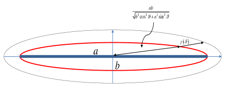
Figure 1: The red ellipse represents the agent trajectory. The area defined by the black curve is the agent’s effective coverage area. $\frac{ab}{\sqrt{b^{2}cos^{2}(\vartheta)+a^{2}sin^{2}(\vartheta)}}+\gamma(\vartheta)$ is the distance between the ellipse center and the coverage area boundary for a given $\vartheta$.

The first assumption simply requires that the sensing range of an agent is continuous and the second that all points in $\Xi$ are treated uniformly (as far as how uncertainty is measured) with respect to an elliptical trajectory centered in this region. The following result establishes the fact that an elliptical trajectory with some $b>0$ can achieve a lower cost than a linear trajectory (i.e., $b=0$) in terms of a long-term average uncertainty per unit area.

Proposition IV.1

Under Assumptions 1-2 and $b\in\mathcal{B}$,

$$\lim_{T\rightarrow\infty,b\rightarrow 0}\frac{\partial J(b)}{\partial b}<0$$

i.e., switching from a linear to an elliptical trajectory reduces the cost in (18).

Proof. Since a linear trajectory is the limit of an elliptical one (with the major axis kept fixed) as the minor axis reaches $b=0$, our proof is based on perturbing the minor axis $b$ away from $0$ and showing that we can then achieve a lower average cost $J$ in (18), as long as this is measured over a sufficiently long time interval.

Obviously, the effective coverage area $\Psi_{\Xi}$ depends on the agent’s trajectory and, in particular, on the minor axis length $b$. From the definition of $\Xi$ in (15), note that $\Psi_{\Xi}$ monotonically increases in $b\in\mathcal{B}$, i.e., $\frac{\partial\Psi_{\Xi}}{\partial b}>0$ and it immediately follows that:

$$\frac{\partial}{\partial b}(\frac{1}{\Psi_{\Xi}})=-\frac{\partial\Psi_{\Xi}}{\partial b}\frac{1}{\Psi_{\Xi}^{2}}<0$$ (19)

We now rewrite the area integral in (18) in a polar coordinate system with $\omega=(\xi,\vartheta)\in\mathbb{R}^{2}$, where $\xi$ is the polar radius and $\vartheta$ is the polar angle:

$$J(b)=\frac{1}{\Psi_{\Xi}}\int_{0}^{T}\int_{0}^{2\pi}\int_{0}^{G(a,b,\vartheta)+\gamma(\vartheta)}R(\xi,\vartheta,t)\xi d\xi d\vartheta dt$$ (20)

where

$$G(a,b,\vartheta)=\frac{ab}{\sqrt{b^{2}\cos^{2}(\vartheta)+a^{2}\sin^{2}(\vartheta)}}$$ (21)

is the ellipse equation in the polar coordinate system and $\gamma(\vartheta)$ is defined for any $(\xi,\vartheta)\in\mathbb{R}^{2}$ as

$$\gamma(\vartheta)=\sup_{\xi}\{Bp(\xi,\vartheta,s(t))>A(\xi,\vartheta)\}-G(a,b,\vartheta)$$ (22)

where $\sup_{\xi}\{Bp(\xi,\vartheta,s(t))>A(\xi,\vartheta)\}$ is the distance between the ellipse center and the furthest point $(\xi,\vartheta)$, for any given $\vartheta$, that can be effectively covered by the agent on the ellipse. Taking partial derivatives in (20) with respect to $b$, we get

$$\frac{\partial J}{\partial b} =-\frac{\partial\Psi_{\Xi}}{\partial b}\frac{1}{\Psi_{\Xi}^{2}}\int_{0}^{T}\int_{\Xi}R\left(\omega,t\right)d\omega dt$$

$$+\frac{1}{\Psi_{\Xi}}\int_{0}^{T}\int_{0}^{2\pi}\left[R\left(G(a,b,\vartheta)+\gamma(\vartheta),\vartheta,t\right)\right.$$

$$\left.\cdot(G(a,b,\vartheta)+\gamma(\vartheta))\cdot\frac{\partial G(a,b,\vartheta)}{\partial b}\right.$$

$$\left.+\int_{0}^{G(a,b,\vartheta)+\gamma(\vartheta)}\frac{\partial R\left(\xi,\vartheta,t\right)}{\partial b}\xi d\xi\right]d\vartheta dt\$$ (23)

Recall that our objective is to show that when we perturb a linear trajectory into an elliptical one, which is achieved by increasing $b$ from $0$ to some small $b_{\epsilon}>0$, we can achieve a lower cost. Thus, we aim to show $\frac{\partial J}{\partial b}|_{b\rightarrow 0}<0$. From (19), the first term of (23) is negative, therefore, we only need to show the second term is non-positive when $b\rightarrow 0$. By the definition (21), observe that when $b\rightarrow 0$, $G(a,b,\vartheta)\rightarrow 0$, and $\frac{\partial G\left(a,b,\vartheta\right)}{\partial b}|_{b\rightarrow 0}=\frac{1}{\sin\vartheta}$, for $\vartheta\neq 0$ and $\pi$; $\frac{\partial G\left(a,b,\vartheta\right)}{\partial b}|_{b\rightarrow 0}=a$ for $\vartheta=0$ or $\pi$. Thus, the double integral of the second term of (23) becomes

$$\int_{0}^{T}\int_{0}^{2\pi}\left[\frac{\gamma(\vartheta)}{\sin\vartheta}R\left(\gamma(\vartheta),\vartheta,t\right)+\int_{0}^{\gamma(\vartheta)}\frac{\partial R\left(\xi,\vartheta,t\right)}{\partial b}\xi d\xi\right]d\vartheta dt$$ (24)

By Assumption 2, $A(\omega)=A(\omega^{\prime})$, where $\omega$ and $\omega^{\prime}$ are symmetric with respect to the center point of the ellipse, thus $A(\xi,\vartheta)=A(\xi,\vartheta+\pi)$. Then, for any uncertainty value $R\left(\gamma(\vartheta),\vartheta,t\right)$ satisfying (3), we can find $R\left(\gamma(\vartheta+\pi),\vartheta+\pi,t\right)$ which is symmetric to it with respect to the center point of the ellipse. Then, from (22) and Fig. 1, note that $\gamma(\vartheta)=\gamma(\vartheta+\pi)$. From the perspective of the point $(\gamma(\vartheta),\vartheta)$, the agent movement observed with an initial position $\rho(0)=\eta$ (following the dynamics in (17)) is the same as the movement observed from $(\gamma(\vartheta+\pi),\vartheta+\pi)$ if the agent starts from $\rho(0)=\eta+\pi$ when $T\rightarrow\infty$, since the cost in (18) is independent of initial conditions as $T\rightarrow\infty$. Thus $R\left(\gamma(\vartheta),\vartheta,t\right)=R\left(\gamma(\vartheta+\pi),\vartheta+\pi,t\right)$. Since, in addition, $\sin\vartheta=-\sin(\vartheta+\pi$), we have $\gamma(\vartheta)\frac{R(\gamma(\vartheta),\vartheta,t)}{\sin\vartheta}=-\gamma(\vartheta+\pi)\frac{R(\gamma(\vartheta+\pi),\vartheta+\pi,t)}{\sin(\vartheta+\pi)}$ and it follows that

$$\lim_{T\rightarrow\infty,b\rightarrow 0}\int_{0}^{T}\int_{0}^{2\pi}\frac{\gamma(\vartheta)}{\sin\vartheta}R\left(\gamma(\vartheta),\vartheta,t\right)d\vartheta dt=0$$ (25)

We now turn our attention to the last integral of (23). Two cases need to be considered here in view of (3):

$(i)$ If $\exists t^{\prime}$ such that $R(\xi,\vartheta,t^{\prime})=0$ for $t^{\prime}\in(0,t)$, then let

$$\tau_{f}(t)=\sup_{\tau\leq t}\{\tau:R(\xi,\vartheta,\tau)=0\}$$ (26)

If $\tau_{f}(t)<t$, then $R(\xi,\vartheta,\tau)>0$ for all $\tau\in[\tau_{f}(t),t)$ and $\tau_{f}(t)$ is the last time instant prior to $t$ when $R\left(\xi,\vartheta,\tau\right)$ leaves an arc such that $R(\xi,\vartheta,\tau)=0$. We can then write $R\left(\xi,\vartheta,t\right)=\int_{\tau_{f}(t)}^{t}\dot{R}\left(\xi,\vartheta,\delta\right)d\delta$. Therefore,

$$\frac{\partial R(\xi,\vartheta,t)}{\partial b} =\frac{\partial t}{\partial b}\dot{R}(\xi,\vartheta,t)-\frac{\partial\tau_{f}(t)}{\partial b}\dot{R}(\xi,\vartheta,\tau_{f}(t))$$

$$+\int_{\tau_{f}(t)}^{t}\frac{\partial\dot{R}(\xi,\vartheta,\delta)}{\partial b}d\delta$$ (27)

Clearly, $\frac{\partial t}{\partial b}=0$ and since $\tau_{f}(t)$ is a time instant when $R(\xi,\vartheta,t)$ leaves $R(\xi,\vartheta,t)=0$ then, by Assumption 1, $\dot{R}(\xi,\vartheta,t)$ is a continuous function and we have $\dot{R}(\xi,\vartheta,\tau_{f}(t))=0$. Therefore, (27) becomes

$$\frac{\partial R(\xi,\vartheta,t)}{\partial b}=\int_{\tau_{f}}^{t}\frac{\partial\dot{R}(\xi,\vartheta,\delta)}{\partial b}d\delta$$ (28)

where, from (3), $\dot{R}(\xi,\vartheta,\delta)=A(\xi,\vartheta)-Bp(\xi,\vartheta,s(\delta))$.

If, on the other hand, $\tau_{f}(t)=t$, then $R(\xi,\vartheta,t)=0$ and we define $\sigma_{f}(t)=\sup_{\sigma\leq t}\{\sigma:R(\xi,\vartheta,\sigma)>0\}$. Proceeding as above, we get

$$\frac{\partial R(\xi,\vartheta,t)}{\partial b}=\int_{\sigma_{f}}^{t}\frac{\partial\dot{R}(\xi,\vartheta,\delta)}{\partial b}d\delta$$

where now $\dot{R}(\xi,\vartheta,\delta)=0$ and we get

$$\frac{\partial R(\xi,\vartheta,t)}{\partial b}=0$$ (29)

$(ii)$ $R(\xi,\vartheta,t^{\prime})>0$ for all $t^{\prime}\in(0,t)$. In this case, we define $\tau_{f}(t)=0$ and we have $R(\xi,\vartheta,t)=R(\xi,\vartheta,0)+\int_{\tau_{f}(t)}^{t}\dot{R}\left(\xi,\vartheta,\delta\right)d\delta$, where $\dot{R}\left(\xi,\vartheta,\delta\right)=A(\xi,\vartheta)-Bp(\xi,\vartheta,s(t)).$ Thus,

$$\frac{\partial R(\xi,\vartheta,t)}{\partial b}=\frac{\partial R(\xi,\vartheta,0)}{\partial b}+\frac{\partial t}{\partial b}\dot{R}(\xi,\vartheta,t)+\int_{\tau_{f}(t)}^{t}\frac{\partial\dot{R}(\xi,\vartheta,\delta)}{\partial b}d\delta$$ (30)

Clearly, $\frac{\partial t}{\partial b}=0$ and $\frac{\partial R(\xi,\vartheta,0)}{\partial b}=0$, since $R(\xi,\vartheta,0)$ is the initial uncertainty value at $(\xi,\vartheta)$ Then, (30) becomes

$$\frac{\partial R(\xi,\vartheta,t)}{\partial b}=\int_{\tau_{f}}^{t}\frac{\partial\dot{R}(\xi,\vartheta,\delta)}{\partial b}d\delta$$ (31)

which is the same result as (28).

Let us start by setting aside the much simpler case where (29) applies and consider (28) and (31). Noting that $\frac{\partial A(\xi,\vartheta)}{\partial b}=0$ we get

$$\frac{\partial\dot{R}\left(\xi,\vartheta,\delta\right)}{\partial b}=-B\frac{\partial p(\xi,\vartheta,s(\delta))}{\partial b}$$ (32)

Recall that $[X,Y]$ has been selected to be the origin and that $\varphi=0$. In this case, (16) becomes

$$s^{x}\left(t\right)=a\cos\rho\left(t\right),\text{ \ \ }s^{y}\left(t\right)=b\sin\rho\left(t\right)$$ (33)

Observing that $s^{x}(t)$ is independent of $b$, (32) gives

$$\frac{\partial\dot{R}\left(\xi,\vartheta,\delta\right)}{\partial b} =-B\frac{\partial p(\xi,\vartheta,s(\delta))}{\partial s^{y}(\delta)}\frac{\partial s^{y}(\delta)}{\partial b}$$

$$=-B\frac{\partial p(\xi,\vartheta,s(\delta))}{\partial D(\xi,\vartheta,s(\delta))}\frac{\partial D(\xi,\vartheta,s(\delta))}{\partial s^{y}(\delta)}\sin\rho(\delta)$$ (34)

where $D(\xi,\vartheta,s(\delta))=[(s^{x}(\delta)-\xi\cos\vartheta)^{2}+(s^{y}(\delta)-\xi\sin\vartheta)^{2}]^{1/2}$, hence

$$\frac{\partial D(\xi,\vartheta,s(\delta))}{\partial s^{y}(\delta)}=\frac{s^{y}(\delta)-\xi\sin\vartheta}{D(\xi,\vartheta,s(\delta))}$$ (35)

Using (35), (34), (28) in the second integral of (24), this integral becomes

$$\int_{0}^{T}\int_{0}^{2\pi}\int_{0}^{\gamma(\vartheta)}\frac{\partial R\left(\xi,\vartheta,t\right)}{\partial b}\xi d\xi d\vartheta dt$$

$$=-B\int_{0}^{T}\int_{0}^{2\pi}\int_{0}^{\gamma(\vartheta)}\xi\int_{\tau_{f}}^{t}\frac{\partial p(\xi,\vartheta,s(\delta))}{\partial D(\xi,\vartheta,s(\delta))}\frac{\left(s_{y}\left(\delta\right)-\xi\sin\vartheta\right)}{D(\xi,\vartheta,s(\delta))}$$

$$\cdot\sin\rho(\delta)d\delta d\xi d\vartheta dt$$ (36)

Note that when $b\rightarrow 0$, we have $s_{y}(\delta)\rightarrow 0$. In addition, $p(\xi,\vartheta,s(\delta))$ is a direct function of $D(\xi,\vartheta,s(\delta))$, so that $\frac{\partial p(\xi,\vartheta,s(\delta))}{\partial D(\xi,\vartheta,s(\delta))}$ is not an explicit function of $\xi,\vartheta$ or $\delta$. Moreover, $\sin\rho(\delta)$ is not a function of $\vartheta$. Thus, switching the integration order in (36) we get

$$B\frac{\partial p(D)}{\partial D}\int_{0}^{T}\int_{\tau_{f}}^{t}\sin\rho\left(\delta\right)\int_{0}^{2\pi}\int_{0}^{\gamma(\vartheta)}\frac{\xi^{2}\sin\vartheta}{D(\xi,\vartheta,s(\delta))}d\xi d\vartheta d\delta dt$$

Using Assumption 2, we make a symmetry argument similar to the one regarding (25). For any point $\omega=(\xi,\vartheta)\in\mathbb{R}^{2}$, we can find $(\xi,\vartheta+\pi)$ which is symmetric to it with respect to the center point of the ellipse and Assumption 2 implies that $A(\xi,\vartheta)=A(\xi,\vartheta+\pi)$. Then, from the perspective of the point $(\xi,\vartheta)$, the agent movement observed with an initial position $\rho(0)=\eta$ (following the dynamics in (17)) is the same as the movement observed from $(\xi,\vartheta+\pi)$ if the agent starts from $\rho(0)=\eta+\pi$ when $T\rightarrow\infty$, since the cost in (18) is independent of initial conditions as $T\rightarrow\infty$. In addition, we again have $\gamma(\vartheta)=\gamma(\vartheta+\pi)$, so that $\int_{0}^{\gamma(\vartheta)}\frac{\sin\vartheta}{D(\xi,\vartheta,s(\delta))}=-\int_{0}^{\gamma(\vartheta+\pi)}\frac{\sin(\vartheta+\pi)}{D(\xi,\vartheta+\pi,s(\delta))}$. Therefore,

$$\lim_{T\rightarrow\infty}\int_{0}^{2\pi}\int_{0}^{\gamma(\vartheta)}\frac{\xi^{2}\sin\vartheta}{D(\xi,\vartheta,s(\delta))}d\xi d\vartheta=0$$ (37)

and the second term of (24) gives

$$\lim_{T\rightarrow\infty,b\rightarrow 0}\int_{0}^{T}\int_{0}^{2\pi}\int_{0}^{\gamma(\vartheta)}\frac{\partial R\left(\xi,\vartheta,t\right)}{\partial b}\xi d\xi d\vartheta dt=0$$ (38)

In view of (25) and (38), we have shown that the second term of (23) is $0$ and we are left with the first negative term from (19), giving the desired result:

$$\lim_{T\rightarrow\infty,b\rightarrow 0}\frac{\partial J(b)}{\partial b}=-\frac{\partial\Psi_{\Xi}}{\partial b}\frac{1}{\Psi_{\Xi}^{2}}\int_{0}^{T}\int_{\Xi}R\left(\omega,t\right)d\omega dt<0$$ (39)

Finally, if (29) applies instead of (28), then (29) and (25) immediately imply that the second term of (23) is $0$, completing the proof. $\blacksquare$

Thus, we have proved that as $T\rightarrow\infty$, when $b$ is perturbed from $0$ to some $b_{\epsilon}>0$, an elliptical trajectory achieves a lower cost than a linear one. In other words, we have shown that elliptical trajectories are more suitable for a 2D mission space in terms of achieving near-optimal results in solving problem P1.

In other words, Prop. IV.1 shows that elliptical trajectories are more suitable for a 2D mission space in terms of achieving near-optimal results in solving problem P1.

V Optimal Elliptical Trajectories

Based on our analysis thus far, we now tackle the problem of determining optimal solutions within the class of elliptical trajectories. Our approach is to associate with each agent an elliptical trajectory, parameterize each such trajectory by its center, orientation and major and minor axes, and then solve P1 as a parametric optimization problem. Note that this includes the possibility that two agents share the same trajectory if the solution to this problem results in identical parameters for the associated ellipses. Choosing elliptical trajectories, which are most likely suboptimal relative to a trajectory obtained through a TPBVP solution of P1, offers several practical advantages in addition to reduced computational complexity. Elliptical trajectories induce a periodic structure to the agent movements which provides predictability. As a result, it is also easier to handle issues related to collision avoidance.

For an elliptical trajectory, the $n$th agent movement is described as in (16) by

$$\left\{\begin{array}[c]{c}s_{n}^{x}\left(t\right)=X_{n}+a_{n}\cos\rho_{n}\left(t\right)\cos\varphi_{n}-b_{n}\sin\rho_{n}\left(t\right)\sin\varphi_{n}\\ s_{n}^{y}\left(t\right)=Y_{n}+a_{n}\cos\rho_{n}\left(t\right)\sin\varphi_{n}+b_{n}\sin\rho_{n}\left(t\right)\cos\varphi_{n}\end{array}\right.$$ (40)

where $[X_{n},Y_{n}]$ is the center of the $n$th ellipse, $a_{n},b_{n}$ are its major and minor axes respectively and $\varphi_{n}\in[0,\pi)$ is its orientation, i.e., the angle between the horizontal axis and the major axis of the $n$th ellipse. Note that the parameter $\rho_{n}(t)\in[0,2\pi)$ is the eccentric anomaly. Therefore, we replace problem P1 by the determination of optimal parameter vectors $\Upsilon_{n}\equiv[X_{n},Y_{n},a_{n},b_{n},\varphi_{n}]^{\mathtt{T}},n=1,\dots,N$, and formulate the following problem P2:

$$\mathbf{P2}:\text{ \ \ }\min_{\Upsilon_{n},n=1,\ldots,N}\text{ \ }J=\int_{0}^{T}\sum_{i=1}^{M}R_{i}(\Upsilon_{1},\ldots,\Upsilon_{N},t)dt$$ (41)

Observe that the behavior of each agent under the optimal ellipse control policy is that of a hybrid system whose dynamics undergo switches when $R_{i}(t)$ reaches or leaves the boundary value $R_{i}=0$ (the “events” causing the switches). As a result, we are faced with a parametric optimization problem for a system with hybrid dynamics. We solve this hybrid system problem using a gradient-based approach in which we apply IPA to determine the gradients $\nabla R_{i}(\Upsilon_{1},\ldots,\Upsilon_{N},t)$ on line (hence, $\nabla J$), i.e., directly using information from the agent trajectories and iterate upon them.

V-A Infinitesimal Perturbation Analysis (IPA)

We begin with a brief review of the IPA framework for general stochastic hybrid systems as presented in [15]. The purpose of IPA is to study the behavior of a hybrid system state as a function of a parameter vector $\theta\in\Theta$ for a given compact, convex set $\Theta\subset\mathbb{R}^{l}$. Let $\{\tau_{k}(\theta)\}$, $k=1,\ldots,K$, denote the occurrence times of all events in the state trajectory. For convenience, we set $\tau_{0}=0$ and $\tau_{K+1}=T$. Over an interval $[\tau_{k}(\theta),\tau_{k+1}(\theta))$, the system is at some mode during which the time-driven state satisfies $\dot{x}\ =\ f_{k}(x,\theta,t)$. An event at $\tau_{k}$ is classified as $(i)$ Exogenous if it causes a discrete state transition independent of $\theta$ and satisfies $\frac{d\tau_{k}}{d\theta}=0$; $(ii)$ Endogenous, if there exists a continuously differentiable function $g_{k}:\mathbb{R}^{n}\times\Theta\rightarrow\mathbb{R}$ such that $\tau_{k}\ =\ \min\{t>\tau_{k-1}\ :\ g_{k}\left(x\left(\theta,t\right),\theta\right)=0\}$; and $(iii)$ Induced if it is triggered by the occurrence of another event at time $\tau_{m}\leq\tau_{k}$. IPA specifies how changes in $\theta$ influence the state $x(\theta,t)$ and the event times $\tau_{k}(\theta)$ and, ultimately, how they influence interesting performance metrics which are generally expressed in terms of these variables.

We define:

$$x^{\prime}(t)\equiv\frac{\partial x(\theta,t)}{\partial\theta},\text{ }\tau_{k}^{\prime}\equiv\frac{\partial\tau_{k}(\theta)}{\partial\theta},\text{ \ \ }k=1,\ldots,K$$

for all state and event time derivatives. It is shown in [15] that $x^{\prime}(t)$ satisfies:

$$\frac{d}{dt}x^{\prime}\left(t\right)=\frac{\partial f_{k}\left(t\right)}{\partial x}x^{\prime}\left(t\right)+\frac{\partial f_{k}\left(t\right)}{\partial\theta}$$ (42)

for $t\in[\tau_{k},\tau_{k+1})$ with boundary condition:

$$x^{\prime}(\tau_{k}^{+})\ =\ x^{\prime}(\tau_{k}^{-})+\left[f_{k-1}(\tau_{k}^{-})-f_{k}(\tau_{k}^{+})\right]\tau_{k}^{\prime}$$ (43)

for $k=0,\ldots,K$, where $\tau_{k}^{-}$ is the left limit of $\tau_{k}$. In addition, in (43), the gradient vector for each $\tau_{k}$ is $\tau_{k}^{\prime}=0$ if the event at $\tau_{k}$ is exogenous and

$$\tau_{k}^{\prime}=-\left[\frac{\partial g_{k}}{\partial x}f_{k}(\tau_{k}^{-})\right]^{-1}\left(\frac{\partial g_{k}}{\partial\theta}+\frac{\partial g_{k}}{\partial x}x^{\prime}(\tau_{k}^{-})\right)$$ (44)

if the event at $\tau_{k}$ is endogenous (i.e., $\ g_{k}\left(x\left(\theta,\tau_{k}\right),\theta\right)=0$) and defined as long as $\frac{\partial g_{k}}{\partial x}f_{k}(\tau_{k}^{-})\neq 0$.

In our case, the parameter vectors are $\Upsilon_{n}\equiv[X_{n},Y_{n},a_{n},b_{n},\varphi_{n}]^{\mathtt{T}}$ as defined earlier, and we seek to determine optimal vectors $\varUpsilon_{n}^{\ast},$ $n=1,\dots,N$. We will use IPA to evaluate $\nabla J(\varUpsilon_{1},\ldots,\varUpsilon_{N})=[\frac{\partial J}{\partial\varUpsilon_{1}},\ldots,\frac{\partial J}{\partial\varUpsilon_{N}}]^{\mathtt{T}}$. From (41), this gradient clearly depends on $\nabla R_{i}(t)=\left[\frac{\partial R_{i}\left(t\right)}{\partial\varUpsilon_{1}},\ldots,\frac{\partial R_{i}\left(t\right)}{\partial\varUpsilon_{N}}\right]^{\mathtt{T}}$. In turn, this gradient depends on whether the dynamics of $R_{i}(t)$ in (3) are given by $\dot{R}_{i}(t)=0$ or $\dot{R}_{i}(t)=A_{i}-BP_{i}\left(\mathbf{s}(t)\right)$. The dynamics switch at event times $\tau_{k}$, $k=1,\ldots,K,$ when $R_{i}(t)$ reaches or escapes from $0$ which are observed on a trajectory over $[0,T]$ based on a given $\varUpsilon_{n},$ $n=1,\dots,N$.

IPA equations. We begin by recalling the dynamics of $R_{i}\left(t\right)$ in (3) which depend on the relative positions of all agents with respect to $[\alpha_{i},\beta_{i}]$ and change at time instants $\tau_{k}$ such that either $R_{i}(\tau_{k})=0$ with $R_{i}(\tau_{k}^{-})>0$ or $A_{i}>BP_{i}\left(\mathbf{s}(\tau_{k})\right)$ with $R_{i}(\tau_{k}^{-})=0$. Moreover, the agent positions $s_{n}\left(t\right)=[s_{n}^{x}(t),s_{n}^{y}(t)]$, $n=1,\ldots,N$, on an elliptical trajectory are expressed using (40). Viewed as a hybrid system, we can now concentrate on all events causing transitions in the dynamics of $R_{i}\left(t\right)$, $i=1,\ldots,M$, since any other event has no effect on the values of $\nabla R_{i}(\Upsilon_{1},\ldots,\Upsilon_{N},t)$ at $t=\tau_{k}$.

For notational simplicity, we define $\omega_{i}=[\alpha_{i},\beta_{i}]\in\Omega$. First, if $R_{i}(t)=0$ and $A(\omega_{i})-BP(\omega_{i},\mathbf{s}(t))\leq 0$, applying (42) to $R_{i}\left(t\right)$ and using (3) gives

$$\frac{d}{dt}\frac{\partial R_{i}(t)}{\partial\varUpsilon_{n}}=0$$ (45)

When $R_{i}(t)>0$, we have

$$\frac{d}{dt}\frac{\partial R_{i}\left(t\right)}{\partial\Upsilon_{n}}=-B\frac{\partial p_{n}\left(\omega_{i},s_{n}\left(t\right)\right)}{\partial\Upsilon_{n}}\textstyle\prod\limits_{d\neq n}^{N}\left[1-p_{d}\left(\omega_{i},s_{d}\left(t\right)\right)\right]$$ (46)

Noting that $p_{n}(\omega_{i},s_{n}(t))\equiv p_{n}(D(\omega_{i},s_{n}(t)))$, we have

$$\frac{\partial p_{n}\left(\omega_{i},s_{n}\left(t\right)\right)}{\partial\varUpsilon_{n}}=\frac{\partial p_{n}(D(\omega_{i},s_{n}(t)))}{\partial D(\omega_{i},s_{n}(t)))}\frac{\partial D(\omega_{i},s_{n}(t))}{\partial\varUpsilon_{n}}$$ (47)

where $D(\omega_{i},s_{n}(t))=[(s_{n}^{x}(t)-\alpha_{i})^{2}+(s_{n}^{y}(t)-\beta_{i})^{2}]^{1/2}$. For simplicity, we write $D=D(\omega_{i},s_{n}(t))$ and we get

$$\frac{\partial D}{\partial\varUpsilon_{n}}=\frac{1}{2D}\left(\frac{\partial D}{\partial s_{n}^{x}}\frac{\partial s_{n}^{x}}{\partial\varUpsilon_{n}}+\frac{\partial D}{\partial s_{n}^{y}}\frac{\partial s_{n}^{y}}{\partial\varUpsilon_{n}}\right)$$ (48)

where $\frac{\partial D}{\partial s_{n}^{x}}=2(s_{n}^{x}-\alpha_{i})$ and $\frac{\partial D}{\partial s_{n}^{y}}=2(s_{n}^{y}-\beta_{i})$. Note that $\frac{\partial s_{n}^{x}}{\partial\varUpsilon_{n}}=[\frac{\partial s_{n}^{x}}{\partial X_{n}},\frac{\partial s_{n}^{x}}{\partial Y_{n}},\frac{\partial s_{n}^{x}}{\partial a_{n}},\frac{\partial s_{n}^{x}}{\partial b_{n}},\frac{\partial s_{n}^{x}}{\partial\varphi_{n}}]^{\mathtt{T}}$ and $\frac{\partial s_{n}^{y}}{\partial\varUpsilon_{n}}=[\frac{\partial s_{n}^{y}}{\partial X_{n}},\frac{\partial s_{n}^{y}}{\partial Y_{n}},\frac{\partial s_{n}^{y}}{\partial a_{n}},\frac{\partial s_{n}^{y}}{\partial b_{n}},\frac{\partial s_{n}^{y}}{\partial\varphi_{n}}]^{\mathtt{T}}$. From (40), for $\frac{\partial s_{n}^{x}}{\partial\varUpsilon_{n}}$, we obtain

$$\frac{\partial s_{n}^{x}}{\partial X_{n}} =1,\text{ \ \ }\frac{\partial s_{n}^{x}}{\partial Y_{n}}=0$$

$$\frac{\partial s_{n}^{x}}{\partial a_{n}} =\cos\rho_{n}\left(t\right)\cos\varphi_{n},\text{ \ \ }\frac{\partial s_{n}^{x}}{\partial b_{n}}=-\sin\rho_{n}\left(t\right)\sin\varphi_{n}$$

$$\frac{\partial s_{n}^{x}}{\partial\varphi_{n}} =-a_{n}\cos\rho_{n}\left(t\right)\sin\varphi_{n}-b\sin\rho_{n}\left(t\right)\cos\varphi_{n}$$

Similarly, for $\frac{\partial s_{n}^{y}}{\partial\varUpsilon_{n}}$, we get $\frac{\partial s_{n}^{y}}{\partial X_{n}}=0,\frac{\partial s_{n}^{y}}{\partial Y_{n}}=1,\frac{\partial s_{n}^{y}}{\partial a_{n}}=\cos\rho_{n}\left(t\right)\sin\varphi_{n},\frac{\partial s_{n}^{y}}{\partial b_{n}}=\sin\rho_{n}\left(t\right)\cos\varphi_{n}$ and $\frac{\partial s_{n}^{y}}{\partial\varphi_{n}}=a_{n}\cos\rho_{n}\left(t\right)\cos\varphi_{n}-b\sin\rho_{n}\left(t\right)\sin\varphi_{n}.$ Using $\frac{\partial s_{n}^{x}}{\partial\varUpsilon_{n}}$ and $\frac{\partial s_{n}^{y}}{\partial\varUpsilon_{n}}$ in (48) and then (47) and back into (46), we can finally obtain $\frac{\partial R_{i}\left(t\right)}{\partial\Upsilon_{n}}$ for $t\in[\tau_{k},\tau_{k+1})$ as

$$\frac{\partial R_{i}\left(t\right)}{\partial\Upsilon_{n}}=\frac{\partial R_{i}\left(\tau_{k}^{+}\right)}{\partial\Upsilon_{n}}+\left\{\begin{array}[c]{cc}0&\text{if }R_{i}\left(t\right)=0,\\ &\text{ }A_{i}\leq BP_{i}\left(\mathbf{s}\left(t\right)\right)\\ \int_{\tau_{k}}^{t}\frac{d}{dt}\frac{\partial R_{i}\left(t\right)}{\partial\Upsilon_{n}}dt&\text{otherwise}\end{array}\right.$$ (49)

where the integral above is obtained from (45)-(47). Thus, it remains to determine the components $\nabla R_{i}(\tau_{k}^{+})$ in (49) using (43). This involves the event time gradient vectors $\nabla\tau_{k}=\frac{\partial\tau_{k}}{\partial\varUpsilon_{n}}$ for $k=1,\ldots,K$, which will be determined through (44). There are two possible cases regarding the events that cause switches in the dynamics of $R_{i}\left(t\right)$:

Case 1: At $\tau_{k}$, $\dot{R}_{i}\left(t\right)$ switches from $\dot{R}_{i}\left(t\right)=0$ to $\dot{R}_{i}\left(t\right)=A_{i}-BP_{i}\left(\mathbf{s}(t)\right)$. In this case, it is easy to see that the dynamics $R_{i}(t)$ are continuous, so that $f_{k-1}(\tau_{k}^{-})=f_{k}(\tau_{k}^{+})$ in (43) applied to $R_{i}(t)\$and we get

$$\nabla R_{i}(\tau_{k}^{+})=\nabla R_{i}(\tau_{k}^{-}),\text{ }i=1,\ldots,M$$ (50)

Case 2: At $\tau_{k}$, $\dot{R}_{i}\left(t\right)$ switches from $\dot{R}_{i}\left(t\right)=A_{i}-BP_{i}\left(\mathbf{s}(t)\right)$ to $\dot{R}_{i}\left(t\right)=0$, i.e., $R_{i}(\tau_{k})$ becomes zero. In this case, we need to first evaluate $\nabla\tau_{k}$ from (44) in order to determine $\nabla R_{i}(\tau_{k}^{+})$ through (43). Observing that this event is endogenous, (44) applies with $g_{k}=R_{i}=0$ and we get

$$\nabla\tau_{k}=-\frac{\nabla R_{i}(\tau_{k}^{-})}{A(\omega_{i})-BP(\omega_{i},\mathbf{s}(\tau_{k}^{-}))}$$ (51)

It follows from (43) that

$$\nabla R_{i}(\tau_{k}^{+})=\nabla R_{i}(\tau_{k}^{-})-\frac{[A(\omega_{i})-BP(\omega_{i},\mathbf{s}(\tau_{k}^{-}))]\nabla R_{i}\left(\tau_{k}^{-}\right)}{A(\omega_{i})-BP(\omega_{i},\mathbf{s}(\tau_{k}^{-}))}=0$$ (52)

Thus, $\nabla R_{i}(\tau_{k}^{+})$ is always reset to $0$ regardless of $\nabla R_{i}(\tau_{k}^{-})$.

Objective Function Gradient Evaluation. Based on our analysis, we first rewrite $J$ in (41) as

$$J(\varUpsilon_{1},\ldots,\varUpsilon_{N})=\sum_{i=1}^{M}\sum_{k=0}^{K}{\displaystyle\int_{\tau_{k}(\varUpsilon_{1},\ldots,\varUpsilon_{N})}^{\tau_{k+1}(\varUpsilon_{1},\ldots,\varUpsilon_{N})}}R_{i}(\varUpsilon_{1},\ldots,\varUpsilon_{N},t)dt$$

and (omitting some function arguments) we get

$$\nabla J={\displaystyle\sum_{i=1}^{M}}{\displaystyle\sum_{k=0}^{K}}\left({\displaystyle\int_{\tau_{k}}^{\tau_{k+1}}}\nabla R_{i}\left(t\right)dt+R_{i}\left(\tau_{k+1}\right)\nabla\tau_{k+1}-R_{i}\left(\tau_{k}\right)\nabla\tau_{k}\right)$$

Observing the cancelation of all terms of the form $R_{i}\left(\tau_{k}\right)\nabla\tau_{k}$ for all $k$ (with $\tau_{0}=0$, $\tau_{K+1}=T$ fixed), we finally get

$$\nabla J(\varUpsilon_{1},\ldots,\varUpsilon_{N})=\sum_{i=1}^{M}\sum_{k=0}^{K}{\displaystyle\int_{\tau_{k}}^{\tau_{k+1}}}\nabla R_{i}\left(t\right)dt$$ (53)

This depends entirely on $\nabla R_{i}\left(t\right)$, which is obtained from (49) and the event times $\tau_{k}$, $k=1,\ldots,K$, given initial conditions $s_{n}\left(0\right)$ for $n=1,\ldots,N$, and $R_{i}\left(0\right)$ for $i=1,\ldots,M$. In (49), $\frac{\partial R_{i}\left(\tau_{k}^{+}\right)}{\partial\Upsilon_{n}}$ is obtained through (50)-(52), whereas $\frac{d}{dt}\frac{\partial R_{i}\left(t\right)}{\partial\Upsilon_{n}}$ is obtained through (45)-(48).

Remark 2. Observe that the evaluation of $\nabla R_{i}\left(t\right)$, hence $\nabla J$, is independent of $A_{i}$, $i=1,\ldots,M$, i.e., the values in our uncertainty model. In fact, the dependence of $\nabla R_{i}\left(t\right)$ on $A_{i}$, $i=1,\ldots,M$, manifests itself through the event times $\tau_{k}$, $k=1,\ldots,K$, that do affect this evaluation, but they, unlike $A_{i}$ which may be unknown, are directly observable during the gradient evaluation process. Thus, the IPA approach possesses an inherent robustness property: there is no need to explicitly model how uncertainty affects $R_{i}(t)$ in (3). Consequently, we may treat $A_{i}$ as unknown without affecting the solution approach (the values of $\nabla R_{i}\left(t\right)$ are obviously affected). We may also allow this uncertainty to be modeled through random processes $\{A_{i}(t)\}$, $i=1,\ldots,M$; in this case, however, the result of Proposition IV.1 no longer applies without some conditions on the statistical characteristics of $\{A_{i}(t)\}$ and the resulting $\nabla J$ is an estimate of a stochastic gradient.

Remark 3. Note that the number of agents affects the number of derivative components in (53), so the complexity of $\nabla J(\varUpsilon_{1},\ldots,\varUpsilon_{N})$ in (53) grows linearly in the number of agents $N$. In addition, the calculation of $\nabla J(\varUpsilon_{1},\ldots,\varUpsilon_{N})$ in (53) grows linearly in $T$, as a longer operation time only implies more events at whose occurrence times $\tau_{k}$ the objective function gradient is updated. In other words, solving the problem using IPA is scalable with respect to the number of agents and the operation time.

V-B Objective Function Optimization

We now seek to obtain $[\varUpsilon_{1}^{\ast},\ldots,\varUpsilon_{N}^{\ast}]$ minimizing $J(\varUpsilon_{1},\ldots,\varUpsilon_{N})$ through a standard gradient-based optimization algorithm of the form

$$[\varUpsilon_{1}^{l+1},\ldots,\varUpsilon_{N}^{l+1}]=[\varUpsilon_{1}^{l},\ldots,\varUpsilon_{N}^{l}]-[\eta_{1}^{l},\ldots,\eta_{N}^{l}]\tilde{\nabla}J(\varUpsilon_{1}^{l},\ldots,\varUpsilon_{N}^{l})$$ (54)

where $\{\eta_{n}^{l}\}$, $l=1,2,\ldots$ are appropriate step size sequences and $\tilde{\nabla}J(\varUpsilon_{1}^{l},\ldots,\varUpsilon_{N}^{l})$ is the projection of the gradient $\nabla J(\varUpsilon_{1},\ldots,\varUpsilon_{N})$ onto the feasible set, i.e., $s_{n}(t)\in\Omega$ for all $t\in[0,T]$, $n=1,\ldots,N$. The optimization algorithm terminates when $|\tilde{\nabla}J(\varUpsilon_{1}^{l},\ldots,\varUpsilon_{N}^{l})|<\varepsilon$ (for a fixed threshold $\varepsilon$) for some $[\varUpsilon_{1}^{\ast},\ldots,\varUpsilon_{N}^{\ast}]$. When $\varepsilon>0$ is small, $[\varUpsilon_{1}^{l},\ldots,\varUpsilon_{N}^{l}]$ is believed to be in the neighborhood of the local optimum, then we set $[\varUpsilon_{1}^{\ast},\ldots,\varUpsilon_{N}^{\ast}]=[\varUpsilon_{1}^{l},\ldots,\varUpsilon_{N}^{l}].$ However, in our problem the function $J(\varUpsilon_{1},\ldots,\varUpsilon_{N})$ is non-convex and there are actually many local optima depending on the initial controllable parameter vector $[\varUpsilon_{1}^{0},\ldots,\varUpsilon_{N}^{0}]$. In the next section, we propose a stochastic comparison algorithm which addresses this issue by randomizing over the initial points $[\varUpsilon_{1}^{0},\ldots,\varUpsilon_{N}^{0}]$ . This algorithm defines a process which converges to a global optimum under certain well-defined conditions.

VI Stochastic Comparison Algorithm for global optimality

Gradient-based optimization algorithms are generally efficient and effective in finding the global optimum when one is uniquely specified by the point where the gradient is zero. When this is not the case, to seek a global optimum one must resort to several alternatives which include a variety of random search algorithms. In this section, we use the Stochastic Comparison algorithm in [16] to find the global optimum. As shown in [16], for a stochastic system, if $(i),$ the cost function $J(\varUpsilon)$ is continuous in $\varUpsilon$ and $(ii),$ for each estimate $\hat{J}(\varUpsilon)$ of $J(\varUpsilon)$ the error $W(\varUpsilon)=\hat{J}(\varUpsilon)-J(\varUpsilon)$ has a symmetric pdf, then the Markov process $\{\varUpsilon_{k}\}$ generated by the Stochastic Comparison algorithm will converge to an $\epsilon-$optimal interval of the global optimum for arbitrarily small $\epsilon>0.$ In short, $\lim_{k\rightarrow\infty}P[\varUpsilon^{k}\in\varUpsilon_{\epsilon}^{\ast}]=1,\text{for any }\epsilon>0$, where $\varUpsilon_{\epsilon}^{\ast}$ is defined as $\varUpsilon_{\epsilon}^{\ast}=\{\varUpsilon|J(\varUpsilon)\leq J(\varUpsilon^{\ast})+\epsilon\}$. Using the Continuous Stochastic Comparison (CSC) Algorithm developed in [16] for a general continuous optimization problem, consider $\varUpsilon\in\Phi$ to be a controllable vector, where $\Phi$ is the bounded feasible controllable parameter space. The Stochastic Comparison Algorithm is presented in Algorithm 1.

Algorithm 1 : Continuous Stochastic Comparison (CSC) Algorithm.

1:  Initialize $\varUpsilon^{0}=\phi^{0},k=0.$

2:  For a given $\varUpsilon^{k}=\phi^{k}$, sample the next candidate point $Z^{k}$ from $\Phi$ according to a uniform distribution over $\Phi.$

3:  For a given $Z^{k}=\zeta^{k}$, set

$$\Upsilon^{k+1}=\left\{\begin{array}[]{cc}Z^{k},&\text{with probability }p^{k}\text{,}\\ \Upsilon^{k},&\text{with probability }1-p^{k}\text{,}\end{array}\right.$$ (55)

where $p^{k}=\{P[\hat{J}(\zeta^{k})<\hat{J}(\phi^{k})]\}^{L_{k}}.$

4:  Replace $k$ by $k+1,$ and go to Step 2.

In the CSC algorithm, the probability $p^{k}$ is actually not calculable, since we do not know the underlying probability functions. However, it is realizable in the following way: both $\hat{J}(\zeta^{k})$ and $\hat{J}(\phi^{k})$ are estimated $L_{k}$ times for an appropriately selected increasing sequence $\{L_{k}\}$. If $\hat{J}(\zeta^{k})<\hat{J}(\phi^{k})$ every time, we set $\varUpsilon^{k+1}=Z^{k}.$ Otherwise, we set $\varUpsilon^{k+1}=\varUpsilon^{k}.$

As discussed in Remark 3, the persistent monitoring problem P2 becomes a stochastic optimization problem if $A_{i}(t)$, $i=1,\ldots,M$, are stochastic processes. However, for the deterministic setting in which all $A_{i}$ are constant, the observed value $\hat{J}$ coincides with the actual value $J$ and a one-time comparison $\hat{J}(\zeta^{k})<\hat{J}(\phi^{k})$ is sufficient to replace $\phi^{k}$ with $\zeta^{k}$ for $\varUpsilon^{k+1}.$ In this case, step 3 in Algorithm 1 becomes, for a given $Z^{k}=\zeta^{k}$:

$$\varUpsilon^{k+1}=\left\{\begin{array}[c]{cc}Z^{k}&\text{if }J(\zeta^{k})<J(\phi^{k})\\ \varUpsilon^{k}&\text{otherwise}\end{array}\right.$$ (56)

and the CSC algorithm in this deterministic setting reduces to a comparison algorithm with multi-starts over the 6-dimensional controllable vector $\Upsilon_{n}\equiv[X_{n},Y_{n},a_{n},b_{n},\varphi_{n},\rho_{n}]^{\mathtt{T}},$ for each ellipse associated with agent $n=1,\dots,N$.

Algorithm 2 : IPA-based Optimization Algorithm using CSC to find $\Upsilon_{n}$, $n=1,\ldots,N.$

1:  Set $\epsilon>0$, $k=0$. Initialize $\varUpsilon^{0}=\phi^{0}$, where $\phi^{0}=[\varUpsilon_{1}^{0},\ldots,\varUpsilon_{N}^{0}].$ Initialize $L_{0}$, where $\{L_{k}\}$ is an appropriately selected increasing sequence.

2:  while $k<K,$ do

3:     For a given $\varUpsilon^{k}=\phi^{k}$,

4:     repeat

5:        Compute $s_{n}(t)$, $t\in[0,T]$ using (40) and $\phi^{k}$ for $n=1,\ldots,N$

6:        Compute $\hat{J}(\phi^{k})$, $\tilde{\nabla}J(\phi^{k})$ and update $\phi^{k}$ through (54).

7:     until $|\tilde{\nabla}J(\phi^{k})|<\epsilon$

8:     Sample the next candidate point $Z^{k}$ from $\Phi$ according to a uniform distribution over $\Phi.$ For a given $Z^{k}=\zeta^{k}$,

9:     repeat

10:        Compute $s_{n}(t)$, $t\in[0,T]$ using (40) and $\zeta^{k}$ for $n=1,\ldots,N$

11:        Compute $\hat{J}(\zeta^{k})$, $\tilde{\nabla}J(\zeta^{k})$ and update $\zeta^{k}$ through (54).

12:     until $|\tilde{\nabla}J(\zeta^{k})|<\epsilon$

13:     Set

$$\Upsilon^{k+1}=\left\{\begin{array}[]{cc}Z^{k},&\text{with probability }p^{k}\text{,}\\ \Upsilon^{k},&\text{with probability }1-p^{k}\text{,}\end{array}\right.$$ (57)

where $p^{k}=\{P[\hat{J}(\zeta^{k})<\hat{J}(\phi^{k})]\}^{L_{k}}.$

14:     Replace $k$ by $k+1$.

15:  end while

16:  Set $\varUpsilon^{\ast}=\varUpsilon^{K}$.

VII Numerical Results

We begin with a two-agent example in which we solve P2 by assigning elliptical trajectories using the gradient-based approach in Section V.B (without the CSC Algorithm 1). The environment setting parameters used are: $r=4$ for the sensing range of agents; $L_{1}=20$, $L_{2}=10$, for the mission space dimensions; and $T=200$. All sampling points $[\alpha_{i},\beta_{i}]$ are uniformly spaced within $L_{1}\times L_{2},$ $i=1,\ldots,M$ where $M=(L_{1}+1)(L_{2}+1)=231.$ Initial values for the uncertainty functions are $R_{i}(0)=2$ and $B=6$, $A_{i}=0.2$ for all $i=1,\ldots,M$ in (3). The results are shown in Fig. 2. Note that the initial conditions were set so as to approximate linear trajectories (red ellipses), thus illustrating Proposition IV.1: we can see that larger ellipses achieve a lower total uncertainty value per unit area. Moreover, observe that the initial cost is significantly reduced, indicating the importance of optimally selecting the ellipse sizes, locations and orientations. The cost associated with the final blue elliptical trajectories in this case is $J_{e}=6.93\times 10^{4}$.

Using the same initial trajectories as in Fig. 2(a), we also used a TPBVP solution algorithm for P1. The results are shown in Fig. 3. The TPBVP algorithm is computationally expensive and time consuming (about 800,000 steps to converge). Interestingly, the solution corresponds to a cost $J_{\text{TPBVP}}=7.15\times 10^{4},$ which is higher than that of Fig. 2 where solutions were restricted to the set of elliptical trajectories. This is an indication of the presence of locally optimal trajectories.

Next, we solve the same two-agent example with the same environment setting using the CSC Algorithm 1. For simplicity, we select the ellipse center location $[X_{n},Y_{n}]$ as the only two (out of six) multi-start components: for a given number of comparisons $Q$, we sample the ellipse center $[X_{n},Y_{n}]\in L_{1}\times L_{2},$ $n=1,\ldots,N,$ using a uniform distribution while $a_{n}=5,b_{n}=2,\varphi_{n}=\frac{\pi}{4},\rho_{n}=0,$ for $n=1,2$ are randomly assigned but initially fixed parameters during the number of comparisons $Q$ (thus, it is still possible that there are local minima with respect to the remaining four components $[a_{n},b_{n},\varphi_{n},\rho_{n}]$, but, clearly, all six components in $\Upsilon_{n}$ can be used at the expense of some additional computational cost.) In Fig. 4, the red elliptical trajectories on the left show the initial ellipses and the blue trajectories represent the corresponding resulting ellipses the CSC Algorithm 1 converges to. Figure 4(b) shows the cost vs. number of iterations of the CSC algorithm. The resulting cost for $Q=300$ is $J_{\text{CSC}}^{\text{Det}}=6.57\times 10^{4}$, where ”Det” stands for a deterministic environment. It is clear from Fig. 4(b) that the cost of the worst local minimum is much higher than that of the best local minimum. Note also that the CSC Algorithm 1 does improve the original pure gradient-based algorithm performance $J_{e}=6.93\times 10^{4}$.

In Fig. 5, the values of $A_{i}$ are allowed to be random, thus dealing with a persistent monitoring problem in a stochastic mission space, where we can test the robustness of the IPA approach as discussed in Remark 2. In particular, each $A_{i}$ is treated as a piecewise constant random process $\{A_{i}(t)\}$ such that $A_{i}(t)$ takes on a fixed value sampled from a uniform distribution over $(0.195,0.205)$ for an exponentially distributed time interval with mean $5$ before switching to a new value. The sequence $\{M_{k}\}$ defining the number of cost comparisons made at the $k$th iteration is set so as to grow sublinearly with $M_{k}=\left\lceil{10\log{k}}\right\rceil,k=2,\ldots,Q$. Note that the system in this case is very similar to that of Fig. 4 where $A_{i}=0.2$ for all $i$ without any change in the way in which $\nabla J(\varUpsilon_{1},\ldots,\varUpsilon_{N})$ is evaluated in executing (54). As already pointed out, this exploits a robustness property of IPA which makes the evaluation of $\nabla J(\varUpsilon_{1},\ldots,\varUpsilon_{N})$ independent of the values of $A_{i}$. All other parameter settings are the same as in Fig. 4. In Fig. 5(a), the red elliptical trajectories show the initial ellipses and the blue trajectories represent the corresponding resulting ellipses the CSC Algorithm 1 converges to. The resulting cost for $Q=300$ in Fig. 5(b) is $J_{\text{CSC}}^{\text{Sto}},=6.60\times 10^{4}$, where ”Sto” stands for a stochastic environment. This cost is almost the same as $J_{\text{CSC}}^{\text{Det}}=6.57\times 10^{4}$, showing that the IPA approach is indeed robust to a stochastic environment setting.

Finally, Fig. 6 shows the TPBVP algorithm result when using the optimal (blue) ellipses in Fig. 4(a) as the initial trajectories. The trajectories the TPBVP solver converges to are shown in red and green respectively for each agent. The corresponding cost in Fig. 6(b) is $J_{\text{TPBVP}}=6.07\times 10^{4},$ which is an improvement compared to $J_{\text{CSC}}^{\text{Det}}=6.57\times 10^{4}$ obtained for elliptical trajectories from the CSC Algorithm 1. Compared to the computationally expensive TPBVP algorithm, the CSC Algorithm 1 using IPA is inexpensive and scalable with respect to $T$ and $N.$ Thus, a combination of the two provides the benefit of offering the optimal elliptical trajectories obtained through the CSC Algorithm 1 (the first fast phase of a solution approach) as initial trajectories for the TPBVP algorithm (the second much slower phase.) This combination is faster than  the original TPBVP algorithm and can also achieve a lower cost compared to CSC Algorithm 1.

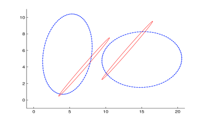
(a) Red ellipses are the initial trajectories and blue ellipses are the final trajectories.

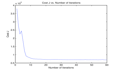
(b) Cost as a function of algorithm iterations. $J_{e}=6.93\times 10^{4}.$

Figure 2: Optimal elliptical trajectories for two agents (without using the CSC algorithm.)

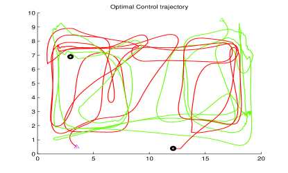
(a) Red and green trajectories obtained from TPBVP solution.

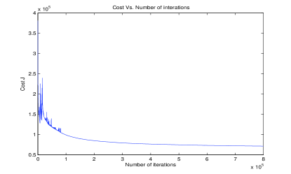
(b) Cost as a function of algorithm iterations. $J_{\text{TPBVP}}=7.15\times 10^{4}.$

Figure 3: Optimal trajectories using TPBVP solver for two agents. Initial trajectories are red curves in Fig. 2(a).

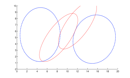
(a) Red ellipses: initial trajectories. Blue ellipses: optimal elliptical trajectories

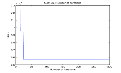
(b) Cost as a function of algorithm iterations. $J_{\text{CSC}}^{\text{Det}}=6.57\times 10^{4}.$

Figure 4: Two agent example for the deterministic environment setting using the CSC Algorithm 1 for $Q=300$ trials.

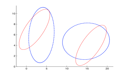
(a) Red ellipses: initial trajectories. Blue ellipses: optimal elliptical trajectories

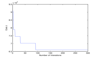
(b) Cost as a function of algorithm iterations. $J_{\text{CSC}}^{\text{Sto}}=6.60\times 10^{4}.$

Figure 5: Two-agent example for a stochastic environment setting using the CSC Algorithm 1 for $Q=300$ trials, where $A_{i}\left(\Delta t_{i}\right)\char 126\relax U\left(0.195,0.205\right)$, $\Delta t_{i}\char 126\relax 0.2e^{-0.2t}$.

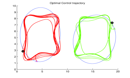
(a) Blue ellipses: initial trajectories. Red and green trajectories: TPBVP converged trajectories.

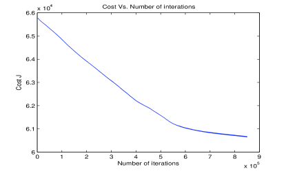
(b) Cost vs. number of iterations. $J_{\text{TPBVP}}=6.07\times 10^{4}.$

Figure 6: Left plot: elliptical trajectories (blue curve) obtained in Fig. 4(a) used as initial trajectories for the TPBVP solver.

VIII Conclusion

We have shown that an optimal control solution to the 1D persistent monitoring problem does not easily extend to the 2D case. In particular, we have proved that elliptical trajectories outperform linear ones in a 2D mission space. Therefore, we have sought to solve a parametric optimization problem to determine optimal elliptical trajectories. Numerical examples indicate that this scalable approach (which can be used on line) provides solutions that approximate those obtained through a computationally intensive TPBVP solver. Moreover, since the solutions obtained are generally locally optimal, we have incorporated a stochastic comparison algorithm for deriving globally optimal elliptical trajectories. Ongoing work aims at alternative approaches for near-optimal solutions and at distributed implementations.

References

- [1] M. Zhong and C. G. Cassandras, “Distributed coverage control and data collection with mobile sensor networks,” Automatic Control, IEEE Transactions on, vol. 56, no. 10, pp. 2445–2455, 2011.
- [2] J. Cortes, S. Martinez, T. Karatas, and F. Bullo, “Coverage control for mobile sensing networks,” IEEE Trans. on Robotics and Automation, vol. 20, no. 2, pp. 243–255, 2004.
- [3] B. Grocholsky, J. Keller, V. Kumar, and G. Pappas, “Cooperative air and ground surveillance,” IEEE Robotics & Automation Magazine, vol. 13, no. 3, pp. 16–25, 2006.
- [4] R. Smith, S. Mac Schwager, D. Rus, and G. Sukhatme, “Persistent ocean monitoring with underwater gliders: Towards accurate reconstruction of dynamic ocean processes,” in IEEE Conf. on Robotics and Automation, 2011, pp. 1517–1524.
- [5] D. Paley, F. Zhang, and N. Leonard, “Cooperative control for ocean sampling: The glider coordinated control system,” IEEE Trans. on Control Systems Technology, vol. 16, no. 4, pp. 735–744, 2008.
- [6] P. Dames, M. Schwager, V. Kumar, and D. Rus, “A decentralized control policy for adaptive information gathering in hazardous environments,” in 51st IEEE Conf. Decision and Control, 2012, pp. 2807–2813.
- [7] S. L. Smith, M. Schwager, and D. Rus, “Persistent monitoring of changing environments using robots with limited range sensing,” IEEE Trans. on Robotics, 2011.
- [8] D. E. Soltero, S. Smith, and D. Rus, “Collision avoidance for persistent monitoring in multi-robot systems with intersecting trajectories,” in Intelligent Robots and Systems (IROS), 2011 IEEE/RSJ International Conference on, 2011, pp. 3645–3652.
- [9] N. Nigam and I. Kroo, “Persistent surveillance using multiple unmanned air vehicles,” in IEEE Aerospace Conf., 2008, pp. 1–14.
- [10] P. Hokayem, D. Stipanovic, and M. Spong, “On persistent coverage control,” in 46th IEEE Conf. Decision and Control, 2008, pp. 6130–6135.
- [11] B. Julian, M. Angermann, and D. Rus, “Non-parametric inference and coordination for distributed robotics,” in 51st IEEE Conf. Decision and Control, 2012, pp. 2787–2794.
- [12] Y. Chen, K. Deng, and C. Belta, “Multi-agent persistent monitoring in stochastic environments with temporal logic constraints,” in 51st IEEE Conf. Decision and Control, 2012, pp. 2801–2806.
- [13] X. Lan and M. Schwager, “Planning periodic persistent monitoring trajectories for sensing robots in gaussian random fields,” in 2013 IEEE International Conference on Robotics and Automation, 2013, pp. 2415–2420.
- [14] C. G. Cassandras, X. Lin, and X. C. Ding, “An optimal control approach to the multi-agent persistent monitoring problem,” IEEE Trans. on Automatic Control, vol. 58, no. 4, pp. 947–961, 2013.
- [15] C. G. Cassandras, Y. Wardi, C. G. Panayiotou, and C. Yao, “Perturbation analysis and optimization of stochastic hybrid systems,” European Journal of Control, vol. 16, no. 6, pp. 642–664, 2010.
- [16] G. Bao and C. G. Cassandras, “Stochastic comparison algorithm for continuous optimization with estimation,” Journal of optimization theory and applications, vol. 91, no. 3, pp. 585–615, December 1996.
- [17] W. Zhang, M. P. Vitus, J. Hu, A. Abate, and C. J. Tomlin, “On the optimal solutions of the infinite-horizon linear sensor scheduling problem,” in 49th IEEE Conf. Decision and Control, 2010, pp. 396–401.
- [18] A. Bryson and Y. Ho, Applied optimal control. Wiley N.Y., 1975.
- [19] X. Lin and C. G. Cassandras, “An optimal control approach to the multi-agent persistent monitoring problem in two-dimensional spaces,” in Proc. of 52nd IEEE Conf. Decision and Control, 2013, pp. 6886–6891.