Near-parabolic comets observed in 2006–2010. The individualized approach to 1/a-determination and the new distribution of original and future orbits

Abstract

Dynamics of a complete sample of small perihelion distance near-parabolic comets discovered in the years 2006 – 2010 are studied (i.e. of 22 comets of $q_{\rm osc}<3.1$ au).

First, osculating orbits are obtained after a very careful positional data inspection and processing, including where appropriate, the method of data partitioning for determination of pre- and post-perihelion orbit for tracking then its dynamical evolution. The nongravitational acceleration in the motion is detected for 50 per cent of investigated comets, in a few cases for the first time. Different sets of nongravitational parameters are determined from pre- and post-perihelion data for some of them. The influence of the positional data structure on the possibility of the detection of nongravitational effects and the overall precision of orbit determination is widely discussed.

Secondly, both original and future orbits were derived by means of numerical integration of swarms of virtual comets obtained using a Monte Carlo cloning method. This method allows to follow the uncertainties of orbital elements at each step of dynamical evolution. The complete statistics of original and future orbits that includes significantly different uncertainties of 1/a-values is presented, also in the light of our results obtained earlier. Basing on 108 comets examined by us so far, we conclude that only one of them, C/2007 W1 Boattini, seems to be a serious candidate for an interstellar comet. We also found that 53 per cent of 108 near-parabolic comets escaping in the future from the Solar system, and the number of comets leaving the Solar system as so called Oort spike comets (i.e. comets suffering very small planetary perturbations) is 14 per cent.

A new method for cometary orbit quality assessment is also proposed by means of modifying the original method, introduced by Marsden et al. (1978). This new method leads to a better diversification of orbit quality classes for contemporary comets.

1 Introduction

The origin of comets is a problem discussed for centuries but still not fully understood. An important element of this puzzle is a question of the observed source of near-parabolic comets. There are two important observational facts that should help us to find an answer. First is the almost perfectly spherically symmetric distribution of their perihelia directions, what has lead Hal Levison (1996) to call these comets nearly isotropic comets (NICs). The second is the striking distribution of their original (i.e. before entering the planetary zone) orbital energies, typically expressed in terms of the reciprocal of the original semimajor axis, see for example Fernández, 2005, page 105. This distribution, highly concentrated near zero, was first pointed out by Oort (1950) and used as an evidence, that the Solar system is surrounded by a huge, spherical cloud of comets, now called the Oort Cloud. Oort analysed the sample of only 19 precise original cometary orbits but since that time hundreds of such orbits were obtained and their $1/a_{\rm{ori}}$ strong concentration in the interval between zero and $100\times 10^{-6}$au^-1 is still evident. Since that time more and more authors call comets with the original semimajor axis in this range the Oort spike comets. This term however, is a source of a serious misunderstanding since a very popular and widely repeated opinion that “Comets in the spike come from the Oort cloud” (see for example Fernández, 2005, page 104) seems to be far-reaching simplification of reality. As early as in 1978 Marsden et al. (hereafter MSE) formulated an opinion, that comets from the Oort spike “are probably making their first passage through the inner part of the solar system”. They stressed (through the use of ’probably’ in italic) that this is only a guess or assumption. This word was omitted in the majority of following papers and now is usually and incorrectly postulated that this is an obvious fact that comets having original barycentric semimajor axis greater than about 10 000 au (or even a few thousand au) are dynamically new. The simplest evidence for this to be erratic is the fact, that a significant percentage of future (when leaving planetary zone) semimajor axes of near-parabolic comets are still in the spike but potential observers during next perihelion passages cannot treat them as making their first visit among planets. The term Solar system transparency i.e. the probability that a near-parabolic comet would pass through the observability zone experiencing infinitesimal planetary perturbations was first proposed and discussed by Dybczyński (2004, 2005) and recently also studied by Fouchard et al., 2013. They showed the dependence of this probability on a perihelion distance and estimated it to vary from almost zero for smallest perihelion distances, through 20 per cent at $q=5$ au up to 70 per cent at $q=10$ au. The study of motion of the observed large perihelion distance LPCs through the zone of strong planetary perturbations, often called the Jupiter–Saturn barrier, was also recently carried by present authors (Dybczyński & Królikowska, 2011, hereafter Paper 2). In the observed sample of LPCs examined by us so far (i.e. 108 LPCs of $1/a_{{\rm ori}}<10^{-4}$ au^-1) we estimated the Solar system transparency to be on the level of 14 per cent.

In the current paper we will use both terms: ’near-parabolic comets’ and ’long period comets’, as well as the abbreviation LPCs, treating them as equivalent.

There is another strong evidence that not all Oort spike comets make their first visit into the planetary zone. The significant per cent of the previous perihelia obtained from the detailed studies of their past dynamical evolution are placed well inside the planetary zone (e.g. Paper 2, and Królikowska & Dybczyński, 2010, hereafter Paper 1). Formulating his hypothesis, Oort (1950) assumed that near-parabolic comets moving on Keplerian orbits outside the planetary perturbation zone are sometimes (mostly near an aphelion) perturbed by passing stars. Since that time, our knowledge on their dynamics has significantly increased, mainly by recognizing the importance of the Galactic perturbations in their motion (see Dones et al., 2004 for a review). Using the first order approximation, one can see that the strength of the Galactic perturbation on a perihelion distance scales with $a^{7/2}$ (Dones et al., 2004). Basing on 53 observed LPCs with $q\geq 3.0$ au we estimated this relation to be $\Delta q\sim a^{4.06\pm 0.16}$, see Paper 2 for details. While early estimations of the Galactic disc matter density $\rho$ lead to the conclusion that for a comet to ’jump over’ the Jupiter-Saturn barrier in one orbital period it is sufficient to have the semimajor axis $a>10\,000$ au, the contemporary value of $\rho=0.100$ M_⊙ pc^-3 makes this limiting semimajor axis value much larger, typically 20 000 – 28 000 au (Levison et al., 2001; Dones et al., 2004; Morbidelli, 2005).

Nowadays it is clear that information about the $1/a_{{\rm ori}}$-value is not sufficient to determine the dynamical status of so-called Oort spike comets and the previous perihelion distance must be inspected as we postulate starting from the paper by Dybczyński (2001) and what previously was discussed by Yabushita (1989). In his paper, Yabushita showed that only 18 of 48 Oort spike comets discovered up to 1989 are dynamically new (less than 40 per cent). However, to know correctly the dynamical status of ’Oort spike’ comet we should follow the cometary orbit to the previous perihelion taking into account not only the Galactic disc tide as Yabushita did in his approximation but also account for the Galactic centre term (Fouchard et al., 2005) and for perturbations from passing stars (Fouchard et al., 2011). Even then we might only know whether the previous perihelion passage of an actual comet was inside the inner part of the Solar system or beyond the planetary zone.

Starting from the classical paper of MSE it becomes clear that an another important factor, namely nongravitational (NG) effects, should be taken into account in the context of the determination of original inverse semimajor axes of near-parabolic comets. As it was already demonstrated by Królikowska (2001, 2002, 2004) the NG accelerations should be included when determining osculating orbits of LPCs, since they can significantly change their original semimajor axes. This effect was also clearly presented in Paper 1.

Therefore, the aim of this paper is twofold.

First, we develop our methods of a precise osculating orbit determination (hereafter a nominal orbit) for the purpose of previous and next perihelion passage calculations, that will be described in the second part of this investigation (Dybczyński & Królikowska, 2013a, hereafter Part II). Here, we try to determine an NG orbit for each investigated here LPC (Section 2) and next we discuss these results with the a priori possibilities of NG determinations based on the data structure (Section 4). For a complete sample of near-parabolic comets observed in 2006 – 2010, and having $q<3.1$ au and $1/a_{{\rm ori}}<150\times 10^{-6}$ au^-1, we notice the 50 per cent of success for the detection of NG effects in comet’s motion using the positional data. Additional result of our study is a new method of cometary orbit quality assessment that is described in details in Section 3.

Secondly, to know the dynamical status in the context of the previous perihelion passage of analysed here comets, we construct a swarm of osculating virtual comets (hereafter VCs) on the basis of the nominal orbit derived previously for each comet. In this part of investigation, we follow each swarm backward and forward to a distance of 250 au from the Sun. Thus, we obtain the original and future orbits for each comet together with the uncertainties of all orbital parameters. The method is described in Section 5. In that section, we focus on two different issues: (i) the change of original inverse semimajor axis due to incorporating the NG acceleration in the osculating orbit determination from the data, and (ii) the statistics of original and future $1/a$-distribution of the sample of 108 near-parabolic comets studied by us here and in our previous papers. In the second aspect, we concentrate on a detailed discussion of original and future $1/a$-distribution as well as the observed planetary perturbation distribution in the context of all so-called Oort spike comets studied by us so far (in Paper 1 & 2). Here, we use the term Oort spike because of its popularity. However, we always have in mind near-parabolic comets, remembering that they consist of two populations of dynamically new and dynamically old comets. We will return to this aspect in Part II.

In Part II, we will follow each swarm of barycentric orbits of VCs (taken at 250 au from the Sun) to the previous and next perihelion taking into account the Galactic perturbations and perturbations of all known stars. Then, we will discuss the observed distribution of Oort spike together with the problem of cometary origin. This paper is in preparation.

Table 1: Description of observational material of 22 LPCs discovered during the period 2006–2010 (columns $[4]-[8]$) and global characteristics of orbits determined here from the entire data intervals (columns $[9]-[10]$). Second and third columns show an osculating perihelion distance and perihelion time, respectively. Data distribution relative to a perihelion passage is presented in columns $[7]$ & $[8]$, where ’pre!’ (’post!’) means that all observations were taken before (after) perihelion passage; ’pre+’ (’post+’) means that we noticed significantly more pre-perihelion (or post-perihelion) measurements, and additional ’$+$’ indicates the drastic dominance of pre-perihelion (or post-perihelion) measurements in both the number and the time interval. Column $[10]$ shows the type of the best model possible to determine from the full interval of data (subscript ’un’ informs that for a given comet the GR and even the NG model determined from the entire interval of data is not satisfactory), and column $[9]$ gives the resulting orbital class determined according to Q^∗ given in column [12] and recipe given in Section 3; notice that the subscript ’un’ in [10] means that due to an inappropriate model the orbital class in a given case is also very preliminary. Column $[11]$ shows our division of investigated comets into four groups (a detailed description is in Section 4.)

Comet	qosc	T	Observational arc	No	Data	Heliocentric	Data	Orbital	Type of	Comet	Q∗
name			dates	of	arc span	distance span	type	class	model	group	eq 8
	[au]	[yyyymmdd]	[yyyymmdd – yyyymmdd]	obs	[yr]	[au]
$[1]$	$[2]$	$[3]$	$[4]$	$[5]$	$[6]$	$[7]$	$[8]$	$[9]$	$[10]$	$[11]$	$[12]$
C/2006 HW51  Siding Spring	2.266	20060929	20060423 – 20070807	187	1.3	2.87 – 4.04	full	1a	GR	C	7.5
C/2006 K3  McNaught	2.501	20070313	20060522 – 20080126	207	1.7	3.95 – 4.13	pre+	1a	NG	B	7.5
C/2006 L2  McNaught	1.994	20061120	20060614 – 20070707	408	1.1	2.74 – 3.31	full	1a	GR	C	7.5
C/2006 OF2  Broughton	2.431	20080915	20060623 – 20100511	4917	3.9	7.88 – 6.31	full	1a+	NG	A	8.5
C/2006 P1  McNaught	0.171	20070112	20060807 – 20070711	341	0.9	2.74 – 3.34	full	1b	NG	B	6.5
C/2006 Q1  McNaught	2.764	20080703	20060820 – 20101017	2744	4.2	6.83 – 7.91	full	1a+	NG	A	9.0
C/2006 VZ13  LINEAR	1.015	20070810	20061113 – 20070814	1173	0.7	3.84 – 1.02	pre++	1b	NGun	D	6.5
C/2007 N3  Lulin	1.212	20090110	20070711 – 20110101	3951	3.2	6.38 – 7.83	full	1a+	NGun	A	8.5
C/2007 O1  LINEAR	2.877	20070603	20060402 – 20071113	183	1.6	4.99 – 2.91	post++	1a	GR	C	7.5
C/2007 Q1  Garradd	3.006	20061211	20070821 – 20070914	43	24d	3.88 – 4.02	post!	3a	GR	D	3.5
C/2007 Q3  Siding Spring	2.252	20091007	20070825 – 20110925	1368	4.0	7.64 – 7.24	full	1a+	NGun	A	9.0
C/2007 W1  Boattini	0.850	20080624	20071120 – 20081217	1703	1.2	3.33 – 2.84	full	1a	NGun	B	7.5
C/2007 W3  LINEAR	1.776	20080602	20071129 – 20080908	212	0.8	2.89 – 2.17	pre+	1b	NG	B	6.5
C/2008 A1  McNaught	1.073	20080929	20080110 – 20100117	937	2.0	3.73 – 5.82	full	1a	NGun	B	8.0
C/2008 C1  Chen-Gao	1.262	20080416	20080130 – 20080528	815	0.3	1.71 – 1.41	pre++	2a	GR	D	6.0
C/2008 J6  Hill	2.002	20080410	20080514 – 20081207	390	0.6	2.04 – 3.41	post!	1b	GR	C	7.0
C/2008 T2  Cardinal	1.202	20090613	20081001 – 20090909	1345	0.9	3.60 – 1.78	pre+	1b	GR	C	7.0
C/2009 K5  McNaught	1.422	20100430	20090527 – 20111028	2539	2.4	4.35 – 6.25	full	1a+	GRun	B	8.5
C/2009 O4  Hill	2.564	20100101	20090730 – 20091214	785	0.4	3.04 – 2.57	pre!	1b	GR	C	6.5
C/2009 R1  McNaught	0.405	20100702	20090720 – 20100629	792	0.9	5.06 – 0.41	pre!	1b	NG	B	7.0
C/2010 H1  Garradd	2.745	20100618	20100219 – 20100702	47	0.2	2.82 – 2.75	full	2b	GR	D	5.0
C/2010 X1  Elenin	0.482	20110910	20101210 – 201107311	2254	0.6	4.22 – 1.04	pre!	1b	GRun	B	7.0

¹   Comet was observed to 7 September, however comet started to disintegrating in August. Thus, the data were taken to the end of July.

2 Observations and osculating orbit determination

We selected all near-parabolic comets discovered during the period 2006–2010 that have small perihelion distances, i.e. $q_{\rm osc}<3.1$ au, and $1/a_{\rm ori}<0.000150$ au^-1. During the same period 23 comets of $q_{\rm osc}\geq 3.1$ au and $1/a_{\rm ori}<0.000150$ au^-1 were detected; five of them were studied in Paper 2 and nine were still observable in November 2012. This means that data sets of these large perihelion comets were incomplete at the moment of this investigation. Therefore, in this study we restricted to complete sample of comets with small perihelion distances.

All results presented in this paper are based on positional data retrieved from the IAU Minor Planet Center in August 2012, except the case of comet C/2010 H1 where we updated the observational data in January 2013 because then four new pre-discovery observations were published at the Web for this comet. Global characteristics of the observational material are given in columns 2–8 of Table 1. Most of comets in the investigated sample were observed on both orbital legs (compare columns 3, 4 and 8), except of five objects. Two of these comets (C/2007 Q1 and C/2008 J6) were discovered after perihelion passage and three (C/2009 O4, C/2009 R1 and C/2010 X1) were not observed after perihelion passage. The last two comets have passed their perihelia close to the Sun at a distance of 0.40 au and 0.48 au, respectively. Comet C/2010 X1 started to disintegrate about one month before perihelion whereas C/2009 R1 was lost after perihelion. We can suspect that C/2009 R1 also did not survive perihelion passage. One can see that for two other comets, C/2006 VZ₁₃ ($q_{\rm osc}=1.01$ au) and C/2008 C1 ($q_{\rm osc}=1.26$ au), the observations stopped shortly after perihelion passage at the distance of 1.02 au and 1.41 au from the Sun, respectively. Thus, also in these two cases, especially for C/2006 VZ₁₃ where the last observation was taken when comet was only about 1 au from the Earth, we can make a guess about their possible break-up.

Comets passing close to the Sun in their perihelia are of special interest because we should suspect detectable influence of NG forces on their motion. It means, however, that the orbit determination for these LPCs is significantly more complicated than for LPCs with large perihelion distances.

The determination of the NG parameters in the motion of LPCs (see Section 2.1) is much more difficult than in the motion of short-period comets mainly due to limited observational material covering one apparition or even just a half apparition, as we have for six comets mentioned above (compare also columns 3,4 and 8 of Table 1). We discussed earlier in Paper 1 that the appropriate processing of astrometric data is very important for this purpose. In particular, the data weighting is crucial for the orbit fitting not only for comets discovered a long time ago but also for currently observed comets. Thus, we adopted here the same, advanced data treatment as in our previous papers. The detailed procedure of weighting is described in Paper1. In this procedure, each individual set of astrometric data has been processed (selected and weighted) during the determination of a pure gravitational orbit (GR) or NG orbit, independently.

Table 2: NG parameters derived in orbital solutions based on entire data intervals. First row of each object presents NG model given also in Table 3. Remaining models are here only to show alternative NG solutions (ignoring normal component of NG acceleration, column $[4]$, and/or assuming the time shift of $g(r)$-function relative to perihelion passage, column $[5]$). Only for C/2006 K3, C/2006 OF₂, C/2006 P1, C/2006 Q1, C/2007 W3 and C/2009 R1 NG models given in the first rows are used as preferred models for studying the dynamical evolution; compare with Table 3.

Comet	NG parameters defined by Eq. 2 in units of 10${}^{-8}\,$au day-2						$\tau$		rms	1/aori
	A1		A2		A3		$[$ days$]$		$[$arcsec$]$	$[$10-6 au${}^{-1}]$
$[1]$	$[2]$		$[3]$		$[4]$		$[5]$		$[6]$	$[7]$
C/2006 K3	15.69 $\pm$	1.67	2.25 $\pm$	2.45	$-$0.209 $\pm$	0.576	–		0.54	61.02 $\pm$	4.63
	15.66 $\pm$	1.67	2.40 $\pm$	2.41	0.0		–		0.55	61.74 $\pm$	4.25
C/2006 OF2	2.384 $\pm$	0.168	$-$1.370 $\pm$	0.131	$-$0.0059 $\pm$	0.0347	–		0.36	21.21 $\pm$	0.49
	2.389 $\pm$	0.166	$-$1.372 $\pm$	0.131	0.0		–		0.36	21.21 $\pm$	0.49
C/2006 P1	0.1329 $\pm$	0.0335	0.03138 $\pm$	0.00397	0.0		–		0.25	57.17 $\pm$	4.03
C/2006 Q1	33.504 $\pm$	0.700	1.916 $\pm$	0.550	10.604 $\pm$	0.189	–		0.37	51.08 $\pm$	0.48
	31.794 $\pm$	0.752	$-$2.710 $\pm$	0.728	10.199 $\pm$	0.189	37.6 $\pm$	4.2	0.37	49.69 $\pm$	0.47
	27.519 $\pm$	0.840	$-$11.592 $\pm$	0.632	0.0		50		0.461	44.28
C/2006 VZ13	1.874 $\pm$	0.804	$-$0.866 $\pm$	0.483	0.528 $\pm$	0.404	–		0.392	13.96 $\pm$	4.80
	1.434 $\pm$	0.686	$-$0.547 $\pm$	0.376	0.0		–		0.392	15.86 $\pm$	4.46
	4.576 $\pm$	0.115	$-$3.041 $\pm$	0.135	1.220 $\pm$	0.074	–		0.51	$-$18.39 $\pm$	3.87
	3.1277 $\pm$	0.0780	$-$1.1912 $\pm$	0.9796	0.0		–		0.54	$-$23.09 $\pm$	4.12
C/2007 N3	0.09377 $\pm$	0.00962	$-$0.00739 $\pm$	0.00611	$-$0.12700 $\pm$	0.00145	–		0.35	32.77 $\pm$	0.18
	0.08678 $\pm$	0.00814	$-$0.02141 $\pm$	0.00696	$-$0.13334 $\pm$	0.00190	11.3 $\pm$	1.9	0.35	32.39 $\pm$	0.17
	0.08650 $\pm$	0.01117	$-$0.01535 $\pm$	0.00961	0.0		11.3		0.491	32.59
C/2007 Q3	0.156 $\pm$	0.180	2.675 $\pm$	0.103	1.657 $\pm$	0.037	–		0.39	39.13 $\pm$	0.49
	0.114 $\pm$	0.239	2.086 $\pm$	0.136	0.0		–		0.48	36.61 $\pm$	0.64
	0.014 $\pm$	0.189	2.589 $\pm$	0.089	1.592 $\pm$	0.037	$-$25.2 $\pm$	5.1	0.39	40.78 $\pm$	0.56
	$-$0.454 $\pm$	0.230	2.080 $\pm$	0.118	0.0		$-$25		0.481	36.90
C/2007 W1	3.9442 $\pm$	0.0125	$-$0.6133 $\pm$	0.0175	$-$0.06023 $\pm$	0.00361	22.32 $\pm$	4.6	0.67	$-$36.56 $\pm$	1.86
	4.0627 $\pm$	0.0193	$-$0.9758 $\pm$	0.0170	$-$0.05387 $\pm$	0.00433	–		0.96	$-$82.30 $\pm$	2.61
C/2007 W3	4.968 $\pm$	0.572	2.248 $\pm$	0.581	$-$1.084 $\pm$	0.316	–		0.52	31.38 $\pm$	3.85
	4.500 $\pm$	0.614	1.822 $\pm$	0.643	$-$0.655 $\pm$	0.503	$-$22 $\pm$	21	0.52	30.70 $\pm$	6.72
	5.458 $\pm$	0.473	0.957 $\pm$	0.279	0.0		$-$22		0.521	25.71
C/2008 A1	5.5964 $\pm$	0.0570	0.7136 $\pm$	0.0384	0.16800 $\pm$	0.00815	5.76 $\pm$	0.6	0.44	123.07 $\pm$	1.50
	5.1495 $\pm$	0.0320	0.9915 $\pm$	0.0201	0.19393 $\pm$	0.00763	–		0.45	120.14 $\pm$	1.56
	5.9732 $\pm$	0.0362	0.3252 $\pm$	0.0216	0.0		10		0.491	113.73
C/2009 R1	5.798 $\pm$	0.490	$-$1.418 $\pm$	0.359	0.776 $\pm$	0.207	–		0.51	12.16 $\pm$	3.29

¹  Best fitting asymmetric NG models (in the sense of minimal value of rms) with assumed A₃=0.0),
²   NG models based on pre-perihelion data only (see also Table 3).                                                                            

2.1 The non-gravitational acceleration in the comet’s motion

To determine the NG cometary orbit we used the standard formalism proposed by Marsden et al. (1973, hereafter MSY) where the three orbital components of the NG acceleration acting on a comet are scaled with a function $g(r)$ symmetric relative to perihelion:

$$F_{i}=A_{\rm i}\cdot g(r) ,\qquad A_{{\rm i}}={\rm\leavevmode\nobreak\ const\leavevmode\nobreak\ \leavevmode\nobreak\ for}\quad{\rm i}=1,2,3,$$ (1)

$$g(r) =\alpha\left(r/r_{0}\right)^{-2.15}\left[1+\left(r/r_{0}\right)^{5.093}\right]^{-4.614},$$ (2)

where $F_{1},\,F_{2},\,F_{3}$ represent the radial, transverse and normal components of the NG acceleration, respectively and the radial acceleration is defined outward along the Sun-comet line. The normalization constant $\alpha=0.1113$ gives $g(1$ AU$)=1$; the scale distance $r_{0}=2.808$ AU. From orbital calculations, the NG parameters $A_{1},A_{2}$, and $A_{3}$ were derived together with six orbital elements within a given time interval (numerical details are described in Królikowska, 2006). The standard NG model assumes that water sublimates from the whole surface of an isothermal cometary nucleus. The asymmetric model of NG acceleration is derived by using $g(r(t-\tau))$ instead of g(r(t)). Thus, this model introduces an additional NG parameter $\tau$ – the time displacement of the maximum of the $g(r)$ relative to the moment of perihelion passage.

Typically, the radial component, $A_{1}$, derived in a symmetric model is positive (reflecting, in average, the stronger sublimation of this part of cometary surface that is directed to the Sun) and dominate in magnitude over the transverse and normal components. This model, however, does not include the possibility of location of an active region(s) on cometary surface. The negative radial component, $A_{1}<0$, derived in this model, would give a first indication for the asymmetric model of g(r) function (with rather large time displacement of a maximum of the $g(r)$ relative to perihelion) or for the existence of active region(s) on comet’s surface. Described model is very successful in representing the astrometric data, thus also in allowing the realistic dynamical evolution predictions. However, this NG force model does not represent an accurate representation of the actual processes taking place in the cometary nucleus (e.g. see Yeomans, 1994). Thus, using this standard model of NG acceleration we can only go as far as a very general and a very qualitative discussion in this field. Therefore, in this paper we place a strong emphasis on orbital dynamics of near-parabolic comets examined here, accounting only for evident physical events, like disruption or fragmentation. For example, in all such cases registered, we notice the coincidence between bursts (or disruptions) and anomalies occurring in O-C-diagram. Therefore, we decided to exclude such data intervals in the process of osculating orbit determination.

In the present investigation we decided to use an NG force model with the smallest number of parameters needed. We tested asymmetric model for several comets from the sample studied here but no improvement was observed. Moreover, in two cases, C/2006 HW₅₁ and C/2006 P1, just two NG parameters were determinable with reasonable accuracy.

For comets with long time sequences of astrometric data (e.g. belonging to comet group A – see column 11 of Table 1) we also tested a more general form of the dependence of NG acceleration on a heliocentric distance:

$$F_{i}=A_{{\rm i}}^{*}\cdot h(r),\qquad A_{{\rm i}}^{*}={\rm\leavevmode\nobreak\ const\leavevmode\nobreak\ \leavevmode\nobreak\ for}\quad{\rm i}=1,2,3.$$ (3)

where we adopted two different form for a dependence of acceleration on a heliocentric distance, $h(r)$, namely: more general $g(r)$-like function, $g^{*}(r)$ (hereafter GEN model type), and Yabushita function, $f(r)$, based on the carbon monoxide sublimation rate (Yabushita, 1996, hereafter YAB model type).

Thus, we consider here also the following two types of NG models:

• GEN:

  $$h(r)=g^{*}(r)=\alpha\left(r/r_{0}\right)^{-m}\left[1+\left(r/r_{0}\right)^{n}\right]^{-k}$$ (4)

• YAB:

  $$h(r)=f(r)=\frac{1.0006}{r^{2}}\times 10^{-0.07395(r-1)}\cdot\left(1+0.0006r^{5}\right)^{-1}$$ (5)

In a GEN type of NG model we have additional four free parameters: scale distance, $r_{0}$, and exponents $n,m,k$. The function $g^{*}(r)$ is normalized similarly as standard $g(r)$ function, thus $\alpha$ is calculated from the condition: $g^{*}({\rm 1au})=1$, also the $f(r)$ function was normalized to unity at $r=1$ au.

In contrast to comets C/2002 T2 and C/2001 Q4 investigated by Królikowska et al. (2012, hereafter Paper 3), we found that GEN and YAB types of NG model did not improve the orbital data fitting for investigated here comets with more than 3 yr interval of data covering the wide range of heliocentric distances (C/2006 OF₂, C/2006 Q1, C/2007 N3 and C/2007 Q3).

We were able to determine the NG effects for 11 of 22 comets discovered in the period 2006–2010 (see next section). As far as we know this is the richest sample of LPCs with NG effects of currently (in February 2013) published in periodicals and on the Web Pages. Many sources of osculating orbits of comets are available only in the Web. From these sources we noticed that Nakano (2013) and Rocher (2013) published NG orbits for largest per cents of comets in comparison to other Web sources. In February 2013 both sources presented NG osculating orbits for six comets from the period of 2006–2010, whereas we determined NG orbits for eleven comets discovered in this period. Additionally, only at Nakano page (2013) and at IAU Minor Planet Center (2013) values of original and future $1/a$ are given; in the second Web source for three comets with NG orbits: C/2007 W1, C/2008 A1 and C/2008 T2. More details about NG models derived in the present studies are given in the next two sections. In Section 5 we discuss the change of the $1/a_{\rm ori}$ due to incorporation of the NG acceleration in the process of osculating orbit determination using the positional data.

2.2 Osculating orbit determination from the full data interval

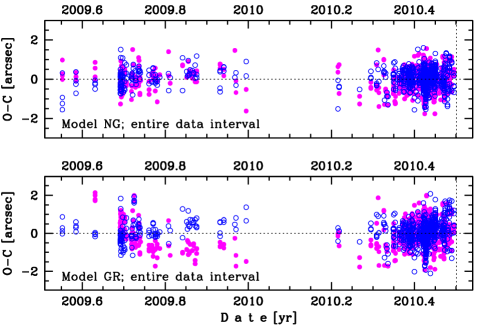
Figure 1: The O-C diagrams for comet C/2009 R1 McNaught (weighted data). The upper figure shows O-C based on an NG solution whereas the lower figure presents O-C based on a pure GR orbit. Residuals in right ascension are shown as magenta dots and in declination – as blue open circles; the moment of perihelion passage is shown by dashed vertical line.

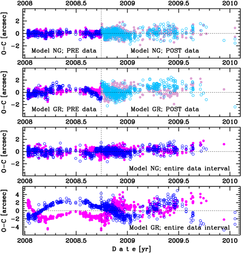
Figure 2: The O-C diagrams for comet C/2008 A1 McNaught (weighted data). Two lower panels show O-C based on the entire data interval for an NG orbit and a pure GR orbit, respectively. Two upper panels present the O-C diagrams for orbits (NG or GR) determined individually for pre-perihelion and post-perihelion orbital branches. Residuals in right ascension are shown as magenta or plum dots and in declination – as blue or light blue open circles; the moment of perihelion passage is shown by dashed vertical line.

We found that NG accelerations are well-detectable in the motion of eleven comets during their periods covered by positional observations. These are comets C/2006 K3, C/2006 OF₂, C/2006 P1, C/2006 Q1, C/2006 VZ₁₃, C/2007 N3, C/2007 Q3, C/2007 W1, C/2007 W3, C/2008 A1, C/2009 R1.

These models are shown as coloured light grey rows in Table 1, whereas the values of original and future 1/a for these models are given in Table 3, except comet C/2006 VZ₁₃ where only the model based on pre-perihelion data are shown for the reason discussed in Section 4.4.

The NG parameters of these symmetric NG models are given in Table 2 in the first row of each individual comet. Additionally, in this table we presented some alternate models that we found as less certain in the sense of orbital fitting to data (three creteria are given just below). Asymmetric NG solution (with $\tau$-parameter, see previous section) was possible to determine for six comets: C/2006 Q1, C/2007 N3, C/2007 Q3 C/2007 W1, C/2007 W3 and C/2008 A1 (see Table 2). However, only in the case of C/2007 W1 we noticed substantial improvement of orbital fitting to data and in the case of C/2008 A1 – the infinitesimal adjustment (in the sense of at least one of three criteria given in section 2.2). For that reason both asymmetric model are also given in Table 3 as the best NG solution derived from the entire data set.

It was surprising that in some cases a normal component od NG acceleration improves the orbit’s fitting to data to the much higher degree than the $\tau$, see the NG solutions for C/2006 Q1, C/2007 N3 and C/2007 Q3. In another words, neglecting the normal component A₃ and determining the A₁, $A_{2}$ and $\tau$ we get the orbital solution with significantly worse data fitting.

One can noticed that almost all these alternate models give original 1/a in a very good agreement with original 1/a-values based on NG models chosen by us to dynamical evolution investigation. The only exception is C/2007 W1 where symmetric model give more hiperbolic orbit that the asymmetric model with $\tau$, however both original 1/a-values are certainly negative. However, this comet exhibits erratic behaviour and its more appropriate solutions (given in the Tables 3 and 6) are discussed later. Comet C/2006 VZ₁₃ is quite a different case because of the almost exclusively pre-perihelion data and some possibility of disintegrating processes close to perihelion.

By ’well-detectable’ NG effects we mean that assuming standard NG model of motion (see Section 2.1) we noticed (for each of these eleven comets) the better orbit fitting to data in comparison to a pure GR orbit measured by three criteria:

• decrease in rms,

• overcoming or reducing the improper trends in O-C time variations,

• increasing the similarity of the O-C distribution to a normal distribution.

More details and examples how this analysis works are given in Papers1–3, therefore only two examples are given below.

Figs 1–2 show the comparison between the O-C diagrams of NG orbit and GR orbit for C/2009 R1 with moderately manifesting NG effects in the motion, and C/2008 A1 with spectacularly visible NG effects in the motion, respectively. We additionally noticed the decrease in rms from 0$.\!\!^{\prime\prime}$63 (GR orbit) to 0$.\!\!^{\prime\prime}$51 (NG orbit) for C/2009 R1 and from 1$.\!\!^{\prime\prime}$44 (GR orbit) to 0$.\!\!^{\prime\prime}$44 (NG orbit) for C/2008 A1. One can see in Fig. 1 that trends easily visible in the O-C diagram based on GR orbit disappear for NG orbit. Moreover at the beginning of the data set, there are four observations taken on 2009 07 20 and four in 2009 08 01. According to our selection procedure all these measurements in right ascension are not used for GR orbit determination due to unacceptable large residuals whereas in the case of NG orbit all are well-fitted as one can see in the upper panel of Fig. 1. Such a data recovery, in particular at the edges of observational period (what we noticed in many cases of the NG orbit determination) is an additional argument for a prevalence of NG orbit (and NG model). Comet C/2008 A1 is a very special case because we still can see in the O-C diagram well-visible trends in residuals in right ascension and declination for NG orbit determined from a whole data set (third panel from the top in Fig 2). Also, the distributions of residuals in $\alpha$ and $\delta$ are not fitted well to normal distributions. Thus, for this comet it was necessary to divide the data into two parts: data before and after perihelion passage. It was very surprising that for both orbital legs the NG orbits were perfectly determinable (both NG solutions are discussed later in this paper). The O-C diagrams for pre-perihelion orbits and post-perihelion orbits are presented in the two upper panels of Fig 2 for NG model and pure GR model, respectively. One can see the great improvements of NG orbit fitting for pre-perihelion data and only slight improvements for post-perihelion data. One can even get an impression that the NG orbit determined from the entire data set (third panel in Fig. 2) gives a better fitting to post-perihelion data that orbit determined from the post-perihelion subset of data. Unfortunately, some trends, in particular in declination, are still noticeable. On the other hand, however, for NG orbit based on post-perihelion data we also noticed the recovery of some measurements taken at the end of observational arc. Thus, we conclude that NG orbit based on the post-perihelion data arc seems to be more adequate to predict the future of this comet as well as the uncertainty of this prediction.

Table 3: Characteristics of models taken in this investigation for previous and next perihelion dynamical evolution. Columns $[3]$ and $[4]$ provide a qualitative assessment of the O-C distribution and O-C diagram, respectively for the types of models given in column [2], where symbol ++ means distributions well-fitted to a normal distribution or O-C diagrams without any meaningful trends in right ascension or/and declination, + denotes distributions rather similar to a Gaussian or O-C diagram with slight trends only, - means non-Gaussian distribution and significant trends in O-C diagram, - - denotes the worse characteristics of O-C distribution or/and O-C diagram. NG models with negative radial component of NG acceleration, $A_{1}<0$, are marked as NG_A1. The rms and a qualitative assessment of O-C distribution are additionally given in columns $[6]$–$[7]$ for GR model based on the same interval of data as NG model given in column $[2]$. A quality class obtained in each individual case as well as the $1/{\rm a}_{{\rm ori}}$ and $1/{\rm a}_{{\rm fut}}$ are given in columns $[8]$–$[10]$, respectively. In the case of PRE-type of model described in columns $[2]$–$[9]$, the type of model used for future $1/a$-determination is listed in column $[11]$.

Comet	Model	Fit to	O-C	rms	rmsGR	GR fit	Orbit	$1/{\rm a}_{{\rm ori}}$		$1/{\rm a}_{{\rm fut}}$		Model type for $1/{\rm a}_{{\rm fut}}$
	type	gauss		′′	′′	to gauss	class	$10^{-6}$ au-1		$10^{-6}$ au-1		if different from $[2]$
$[1]$	$[2]$	$[3]$	$[4]$	$[5]$	$[6]$	$[7]$	$[8]$	$[9]$		$[10]$		$[11]$
2006 HW51	GR	+	+	0.29			1a	47.31 $\pm$	3.37	90.12 $\pm$	3.37
	NGA1	++	++	0.28	0.29	+	1a	30.32 $\pm$	4.40	37.45 $\pm$	8.34
	PRE GR	+	++	0.29			2a	24.84 $\pm$	6.19
2006 K3	NG	++	++	0.54	0.69	+	1a	61.02 $\pm$	$\pm$  4.63	$-$131.28 $\pm$	$\pm$  4.67
2006 L2	GR	++	+	0.49			1a	12.89 $\pm$	1.43	$-$95.28 $\pm$	1.43
	NGA1	+	++	0.46	0.49	++	1a	43.56 $\pm$	4.21	$-$170.88 $\pm$	7.73
	PRE GR	++	++	0.37			1b	63.56 $\pm$	4.52
2006 OF2	NG	++	+	0.36	0.38	-	1a+	21.21 $\pm$	$\pm$  0.49	$-$658.82 $\pm$	$\pm$  0.23
	PRE GR	++	+	0.36			1a	16.42 $\pm$	0.62
2006 P1	NG	+	+	0.25	0.25	+	1b	57.17 $\pm$	$\pm$  4.03	467.65 $\pm$	$\pm$  3.56
2006 Q1	NG	+	++	0.37	0.50	-	1a+	51.08 $\pm$	$\pm$  0.48	707.44 $\pm$	$\pm$  0.31
	PRE GR	+	++	0.34			1a	49.44 $\pm$	0.45
2006 VZ13	PRE NG	++	+	0.39	0.40	+	2a	13.96 $\pm$	4.80	491.21 $\pm$	20.10	NG, class: 1b
2007 N3	PRE GR	-	+	0.33			1a	29.31 $\pm$	0.59	823.61 $\pm$	2.06	POST GR 1, class: 1a
	NG	++	+	0.35	0.50	-	1a+	32.77 $\pm$	$\pm$  0.18	828.64 $\pm$	$\pm$  0.59
2007 O1	GR	++	+	0.47			1a	23.36 $\pm$	4.70	$-$496.83 $\pm$	4.69
2007 Q1	GR	+	+	0.58			3a	54.95 $\pm$	799.09	$-$449.88 $\pm$	741.43
2007 Q3	PRE GR	+	+	0.39			1a+	41.91 $\pm$	0.53	131.77 $\pm$	3.63	POST GR, class: 1a
	NG	+	-	0.39	0.49	-	1a+	39.13 $\pm$	$\pm$  0.49	118.96 $\pm$	$\pm$  0.96
2007 W1	PRE NG	+	+	0.49	0.61	- -	1b	$-$42.71 $\pm$	2.34	554.38 $\pm$	7.09	POST NG, class: 2a
	NG$+\tau$  2	-	-	0.67	2.96	- -	1a	$-$36.56 $\pm$	$\pm$  1.86	549.97 $\pm$	$\pm$  5.79
2007 W3	NG	++	+	0.52	0.54	++	1b	31.38 $\pm$	$\pm$  3.85	343.89 $\pm$	$\pm$ 18.10
2008 A1	PRE NG	++	++	0.28	0.47		1b	120.84 $\pm$	2.03	246.52 $\pm$	2.82	POST NG, class: 1b
	NG$+\tau$  2	+	-	0.44	1.44	- -	1a	123.07 $\pm$	$\pm$ 1.50	256.41 $\pm$	$\pm$ 2.24
	NG	+	-	0.45	1.44	- -	1a	120.14 $\pm$	1.56	247.21 $\pm$	1.89
2008 C1	GR	++	++	0.36			2a	38.57 $\pm$	11.77	502.56 $\pm$	11.77
	NG	++	++	0.36	0.36	++	2a	115.95 $\pm$	59.16	648.87 $\pm$	221.41
2008 J6	GR	++	+	0.47			1b	25.35 $\pm$	4.00	$-$479.69 $\pm$	3.99
2008 T2	GR	++	+	0.38			1b	12.22 $\pm$	1.06	275.92 $\pm$	1.06
	NGA1	++	++	0.39	0.38	++	1b	19.19 $\pm$	1.14	218.90 $\pm$	7.83
	PRE GR	++	++	0.39			1b	11.47 $\pm$	1.08
2009 K5	PRE GR	-	+	0.33			1a	45.50 $\pm$	0.55	552.91 $\pm$	0.41	POST GR, class: 1a
	GR	-	-	0.47		- -	1a+	49.42 $\pm$	0.22	554.68 $\pm$	0.22
	DIST NGA1	+	++	0.39	0.38	- -	1a	44.22 $\pm$	2.75	550.33 $\pm$	1.60
2009 O4	GR	+	++	0.39			1b	55.96 $\pm$	4.91	$-$55.96 $\pm$	4.91
2009 R1	NG	++	++	0.51	0.63	+	1b	12.16 $\pm$	$\pm$  3.29	170.43 $\pm$	$\pm$ 197.25
2010 H1	GR	+	+	0.83			2b	240.15 $\pm$	75.41	784.70 $\pm$	75.46
2010 X1	GRMay	+	+	0.46			1b	24.10 $\pm$	2.20	disintegration
	GRApr	++	++	0.37			1b	27.24 $\pm$	3.95

¹  Model based on data started from heliocentric distance of 2.0 au from the Sun
    ²  Asymmetric models relative to perihelion passage based on entire data sets

The most manifesting NG accelerations we found in C/2007 W1 case where a similar approach was necessary to be used as for C/2008 A1. The same method was applied earlier for C/2007 W1 by Nakano (2009a; 2009b). We found that the orbit obtained on the basis of the whole data set proved to be inadequate to describe the actual motion of both comets (C/2007 W1 and C/2008 A1). We noticed this fact by subscript ’un’ (i.e. uncertain) in column [10] of Table 1. Among comets with very long data intervals ($>$ 3 yr) there are two other objects (C/2007 N3 and C/2007 Q3) with well visible trends in O-C diagrams taken for NG orbit and based on the full observational interval. Therefore, for these two comets it was also necessary to determine the osculating orbit from pre- and post-perihelion subsets of data, independently. Further, in the comet C/2006 VZ₁₃ case, an adequate NG orbit for past dynamical evolution were determined only for some part of pre-perihelion data (ending 40 days before perihelion passage).

Analysing orbits of eleven comets with well-detectable NG effects in their orbital motion we concluded that the motion of six of them can be model by one set of NG parameters during the period covered by data. In the case of remaining five comets the NG behaviour is more complicated. Thus, we proposed in these cases to model their motion separately before and after perihelion passage.

It turn out that NG effects are easily visible in the time interval covered by positional observations also in the motion of comet C/2010 X1. However, this is very special case because the nature of this NG behaviour is likely to be violent – this comet started to disintegrate at least about one months before perihelion passage (in August 2011). Therefore, the NG model used here is completely inadequate (see also Section 4.2). Thus, we modelled the motion of this comet based on the shorter interval of data, e.g. carried out before the disintegration process was started. It turn out, that the best orbit (GR orbit), for the past evolution was determined from an arc of data limited to the observations taken before 1 May 2011 what can suggest that a disruption started even before August 2011. For this reason we also marked the GR solution based on almost entire data interval by subscript ’un’ in Table 1.

For other three comets, C/2006 HW₅₁, C/2006 L2 and C/2008 T2, the NG effects are worse detectable than in previous cases. Additionally, the radial component of standard NG acceleration, A₁ (see Eq. 2), is negative for these objects (see also Section 2.1). However, the GR orbit is quite acceptable since only slight trends are visible in the O-C diagrams of these comets. Therefore, we discussed for them the GR orbit (Table 1) as at least similarly likely solution as NG orbit (Table 3) and included to the group of comets with weak NG effects (Section 4.3).

Comet C/2009 K5 also have marginally detectable NG effects with a negative A₁ but it differs from the previous three comets in visible trends in the O-C diagrams for GR orbit as well NG orbit. Thus, we included this comet to special objects (marked by subscript ’un’ in column $[10]$ of Table 1) where it was necessary to divide the data into pre-perihelion and post-perihelion orbital branches (see Section 4.2).

An interesting example is comet C/2008 C1 that has marginally detectable NG effects. This is surprising because of short interval of data (0.3 yr). We decided to use the GR solution as more reliable for this comet of second quality orbit (Table 1).

NG effects are completely not detectable in the orbital motion of five comets, C/2007 O1, C/2007 Q1, C/2008 J6, C/2009 O4, C/2010 H1, and for these objects we have just pure GR osculating orbits (Table 1). All these comets have osculating perihelion distance ${\rm q}_{{\rm osc}}>2$ au and two of them have poor quality orbits (see Table 1).

2.3 Osculating orbit determination from some part of data

According to the brief overview of orbital determination given in Section 2.2 we have seven special comets, C/2006 VZ₁₃, C/2007 N3, C/2007 Q3, C/2007 W1, C/2008 A1, C/2009 K5 and C/2010 X1, where we have to apply a non-standard approach and determine two individual osculating orbits (GR or NG if possible) for two orbital legs. These solutions were marked as PRE and POST models in column $[2]$ of Table 3. For C/2009 K5 we additionally presented DIST model based on data taken from the heliocentric distances larger than $r_{h}>2.5$ au.

For the remaining comets we noticed that osculating orbits (GR or NG, see Table 1) based on the entire data interval well represent their orbital motion in the period covered by observations. However, for some of these comets (wherever we though it relevant and meaningful) we also determined the osculating orbits based on only a subset of pre-perihelion measurements (i.e. for C/2006 OF₂, C/2006 Q1 and C/2008 C1). These additional orbital solutions are presented here just for comparison and wider discussion of the dynamical evolution of each comet carried out in Part II. Moreover, as was discussed in Section 2.2, for comets C/2006 HW₅₁, C/2006 L2 and C/2008 T2 the NG models based on entire set of data (where radial component of NG acceleration is negative) are also given just for comparison.

Generally, in Table 3 are presented all models (of osculating orbit) taken further in the second part of this investigation for previous and next perihelion dynamical evolution. The best model derived for each comet is given always in the first row and just these best models are used in Section 5 for statistical analysis. The NG models based on the entire data sets are shown in coloured light grey rows, similarly as in Table 1.

3 Accuracy of the cometary orbit

Table 4: Quantities for establishing accuracy of orbit. Slightly modified new version of Table II from MSE

$L$ & $M$	Mean error of 1/aosc		time span of observations
	in units of $10^{-6}$ au-1		in months or days
8			$\geq$ 48 months
7	$<$ 1		$[$24 ,	48$[$
6	$[$1 ,	5$[$	$[$12 ,	24$[$
5	$[$5 ,	20$[$	$[$ 6 ,	12$[$
4	$[$20 ,	100$[$	$[$ 3 ,	6$[$
3	$[$100 ,	500$[$	$[$1.5 ,	3$[$
2	$[$500 ,	2500$[$	$[$23 days ,	1.5 months$[$
1	$[$2 500 ,	12 500$[$	$[$12 ,	23$[$ days
0	$\geq$ 12 500		$[$7 ,	12$[$
-1			$[$3 ,	7$[$
-2			$[$1 ,	3$[$

In 1978 MSE formulated the recipe to evaluate the accuracy of the osculating cometary orbits obtained from the positional data. They proposed to measure this accuracy by the quantity $Q$ defined as

$$Q=1/2\cdot(L+M+N)+\delta,{\rm\leavevmode\nobreak\ \leavevmode\nobreak\ \leavevmode\nobreak\ where}$$ (6)

$L$ denotes a small integer number which depends on the mean error of the determination of the osculating 1/a,

$M$ – a small integer number which depends on the time interval covered by the observations,

$N$ – a small integer number that reflects the number of planets, whose perturbation were taken into account, and

$\delta$ equals 0.5 or 1 to make $Q$ an integer number.

Values of $L$, $M$ and $N$ are obtained following the scheme presented in their original Table II (MSE). According to MSE the integer $Q$-value calculated from Eq. 6 should be next replaced with the orbit quality class as follows: value of $Q=9,8$ means orbit of 1A orbital class, $Q=7$ – 1B class, $Q=6$ – 2A class, $Q=5$ – 2B class, and $Q<5$ means the worse than second class orbit.

There are three reasons for which we found that some slight, but important adjustment of the above orbital accuracy assessment should be done:

1. In the modern orbit determination all Solar system planets are taken into account, therefore we always have $N=3$. Thus, Eq. 6 can be rewritten for our purpose in a form:

   $$Q=Q^{*}+\delta,{\rm\leavevmode\nobreak\ \leavevmode\nobreak\ where\leavevmode\nobreak\ \leavevmode\nobreak\ }$$

   $$Q^{*}=0.5\cdot(L+M+3){\rm\leavevmode\nobreak\ \leavevmode\nobreak\ \leavevmode\nobreak\ \leavevmode\nobreak\ and\leavevmode\nobreak\ \leavevmode\nobreak\ \leavevmode\nobreak\ \leavevmode\nobreak\ }\delta=1{\rm\leavevmode\nobreak\ \leavevmode\nobreak\ \leavevmode\nobreak\ or\leavevmode\nobreak\ \leavevmode\nobreak\ \leavevmode\nobreak\ }0.5$$ (7)

2. Current cometary observations are generally of a high precision and the resulting osculating 1/a-uncertainties are often smaller than 10^-6 au^-1. It should be reflected in a higher $L$ number than is allowed in the original MSE table. Similarly, a higher $M$ number should be attributed to very long time intervals covered by contemporary positional observations of LPCs. Thus, the mean error of $1/a_{\rm osc}$ smaller than 1 unit (i.e. $1\times 10^{-6}$ au^-1) gives now $L=7$ and a time span of data can be greater than 48 months ($M=8$, see Table 4).

3. Almost all orbits of currently discovered LPCs would be classified as the 1A quality class. For example, we found that using the original $\delta$ definition (to be 0.5 or 1) we obtained 15 comets of orbital class 1A and just two comets (C/2007 Q1 and C/2010 H1) of an obvious cases of second or worse orbital class (extremely short orbital arcs) for the sample studied here. Thus, additional modification seems to be necessary to obtain a better diversification of orbit accuracy classes. We proposed below, the new $\delta$ definition and division the first quality class into three new classes (1a+, 1a, 1b) instead former 1A and 1B.

Thus, the more relevant definition of $Q$ for currently discovered LPCs takes the form:

$$Q=Q^{*}+\delta,{\rm\leavevmode\nobreak\ \leavevmode\nobreak\ where\leavevmode\nobreak\ \leavevmode\nobreak\ }$$

$$Q^{*}=0.5\cdot(L+M+3){\rm\leavevmode\nobreak\ \leavevmode\nobreak\ \leavevmode\nobreak\ \leavevmode\nobreak\ and\leavevmode\nobreak\ \leavevmode\nobreak\ \leavevmode\nobreak\ \leavevmode\nobreak\ }\delta=0{\rm\leavevmode\nobreak\ \leavevmode\nobreak\ \leavevmode\nobreak\ or\leavevmode\nobreak\ \leavevmode\nobreak\ \leavevmode\nobreak\ }0.5$$ (8)

How to calculate the quantities $L$ and $M$ is described in Table 4 that is a simpler form of original Table II given by MSE. Value of $\delta$ equals 0.5 or 0 to make $Q$ an integer number. When $Q^{*}$ is an intermediate between two integers (that define two consecutive orbital classes) the proposed new recipe gives the final $Q$-values exactly the same as originally proposed by MSE.

To distinguish the proposed quality system from MSE system, we use lower-case letter ’a’ and ’b’ in quality class descriptions instead of original ’A’ and ’B’ in the following way: $Q=9$ – 1a+ class, $Q=8$ – 1a class, $Q=7$ – 1b class, $Q=6$ – 2a class, $Q=5$ – 2b class, $Q=4$ – 3a class, $Q=3$ – 3b class, and $Q\leq 2$ – 4 class, where $Q$ is calculated according to eq. 8. We additionally propose to introduce a special 1a+ quality class in case of $Q=9$. The quality classes 3a, 3b and 4 were not defined by MSE, but we adopted here the idea published by Minor Planet Center (at http://www.minorplanetcenter.net/iau/info/UValue.html) as ’a logical extension to the MSE scheme’.

This new orbit quality scheme separates the orbits of a very good quality in MSE system, 1A, into three quality classes in the new system, where the worst of orbits in 1A class (Q^∗=7) in MSE are classified as 1b in the new scheme. The reader can check how it works using the Q^∗ value given in last column of Table 1 to calculate the MSE quality class.

In the MWC 08 only pure GR orbits are classified according to MSE method. It seems, however, that there are no contraindications to use such a procedure to qualify also NG orbits. These NG orbits are often of a lower quality than GR orbit obtained on the basis of the same time interval. This is an obvious consequence of higher uncertainties of NG orbital elements as a result of additional NG parameters to determine simultaneously with six orbital elements. In our opinion, the quality comparison between GR orbit and NG orbit should not be carried out exclusively on the basis of an orbital quality because NG orbit is always closer to reality by its physical assumptions, and therefore is more appropriate to describe the cometary motion than GR orbit. On the other hand, a quality assessment for NG orbit gives an easy indication of the uncertainty of orbital elements.

It is worth to stress, that any effective orbit quality assessment system (including the MSE method and this proposed here) describes a particular orbital solution based on a given data set (or subset), procedure used for this data processing as well as the adopted force model. Therefore, orbit of each individual comet can be classified differently, depending on the preferred orbital solution.

3.1 Application of the modified method of orbital quality assessment to comets considered so far

The new modified MSE procedure described above, was applied for the determination of orbital classes of all osculating orbits of the investigated here comets. The results are given in columns 12 and 9 of Table 1 and in column 8 of Table 3. As was mentioned above, one can notice the higher diversification in orbital classes between investigated comets than using the original MSE recipe. This can easily be checked using Eq. 7 and values given in column 12 of Table 1. According to the proposed method we have a lower fraction of comets of the best orbital classes: 11 (1a+ and 1a classes) instead of 15 (1A class). Additionally, these 11 comets are now divided into 5 comets of 1a+ class and 6 comets of 1a class when using entire data sets shown in Table 1. Moreover, the orbit of one comet, C/2008 C1, is reclassified as a second class orbit.

We noticed that at the IAU Minor Planet Center web pages orbital quality codes are given also for newly discovered comets. In February 2013, for five comets investigated in this paper, the quality codes are not shown, namely for C/2007 Q1 (extremely short arc of data) C/2007 W1 (NG orbit), C/2008 A1 (NG orbit), C/2008 T2 (NG orbit with negative radial component of NG acceleration) and C/2010 X1. The remaining 17 objects are classified as follows: 13 comets have 1A class, 2 comets – class 1B (C/2006 VZ₁₃, C/2010 H1), and 2 objects – of class 2A (C/2008 C1, C/2009 O4). We also estimated the orbit of C/2008 C1 as a 2a quality class, but orbit of C/2009 O4 as 1b class. However, 2A quality code for C/2009 O4 is there a natural consequence of shorter intervals of data taken for orbit determination than in the present investigation. Similarly, the JPL Small-Body Database Browser (2013) shows (in February 2013) the osculating orbits on the basis of full interval of positional data.

Table 5: New quality class assessment for 86 near-parabolic comets investigated in Paper1&2

C/	Class	C/	Class	C/	Class	C/	Class
37 comets of NG orbits
$q_{{\rm osc}}<3.1$ au
1885 X1	2a	1892 Q1	2a	1913 Y1	1b	1940 R2	2a
1946 U1	1b	1952 W1	2a	1956 R1	1b	1959 Y1	2b
1974 F1	1a	1978 H1	1b	1986 P1	1a	1989 Q1	2a
1989 X1	1b	1990 K1	1a	1991 F2	1b	1993 A1	1a
1993 Q1	1b	1996 E1	1b	1997 J2	1a+	1999 Y1	1a+
2001 Q4	1a+	2002 E2	1b	2002 T7	1a+	2003 K4	1a+
2004 B1	1a+
$q_{{\rm osc}}\geq 3.1$ au
1980 E1	1a+	1983 O1	1a	1984 W2	1a	1997 BA6	1a+
1999 H3	1a	2000 CT54	1a+	2000 SV74	1a+	2002 R3	1a
2005 B1	1a+	2005 EL173	1a+	2005 K1	1a	2006 S2	1b
49 comets of GR orbits
$q_{{\rm osc}}<3.1$ au
1992 J1	1a+	2001 K3	2a
$q_{{\rm osc}}\geq 3.1$ au
1972 L1	1a	1973 W1	1b	1974 V1	1b	1976 D2	1a
1976 U1	1b	1978 A1	1a	1978 G2	1b	1979 M3	1b
1987 F1	1a	1987 H1	1a+	1987 W3	1a	1988 B1	1a
1993 F1	1a	1993 K1	1a	1997 A1	1b	1999 F1	1a+
1999 F2	1a	1999 J2	1a+	1999 K5	1a+	1999 N4	1a
1999 S2	1a	1999 U1	1a	1999 U4	1a+	2000 A1	1a
2000 K1	1a	2000 O1	1a	2000 Y1	1a	2001 C1	1a
2001 G1	1a	2001 K5	1a+	2002 A3	1a	2002 J4	1a
2002 J5	1a+	2002 L9	1a+	2003 G1	1a	2003 S3	1a
2003 WT42	1a+	2004 P1	1a	2004 T3	1a	2004 X3	1a
2005 G1	1a	2005 Q1	1a	2006 E1	1a	2006 K1	1a+
2006 YC	2a	2007 JA21	1a	2007 Y1	2a

We also applied the modified method of orbital quality determination to pure GR as well as NG orbits of comets from Papers 1 & 2, where all those Oort spike comets were chosen from MWC 08 as objects with highest quality orbits (classes 1A or 1B). The full list of these new quality class assessment for the entire sample of near-parabolic comets is given in Table 5. An extended table, for 108 LPCs investigated by us that includes details about the observational material used for orbit determination, type of models used, as well as the orbit quality estimation, is available in our web page (Dybczyński & Królikowska, 2013b).

It turned out that among 37 comets with NG orbits, six (C/1885 X1, C/1892 Q1, C/1940 R2, C/1952 W1, C/1959 Y1 and C/1989 Q1) should be classified as second quality orbit according to a modified, more restrictive method proposed here (Table 5). Next three with pure GR orbit are now also class 2 objects (C/2001 K3, C/2006 YC and C/2007 Y1).

Summarizing, according to a more restrictive orbital quality assessment proposed here we obtained 23 comets of 1a+ class, 38 comets of 1a class, 16 – 1b class, 8 – 2a class, and 1 object of 2b class in the sample of 86 comets analysed in Papers 1 & 2 that were chosen from MWC 08 as Oort spike comets having pure GR orbit of the highest quality (class 1) or NG orbit (then the quality class is not specified in the catalogue).

4 Implication of data structure on orbit determination

In this section we show how the data structure influence the proper choice of the tailored orbit determination method, how it affects the quality of osculating orbits and the possibility of the determination of NG effects in the motion of near-parabolic comet. We performed an extensive review and tests of various models for each of investigated comets, including asymmetric ones (i.e. NG models with $\tau$-shift of maximum of $g(r)$-function relative to perihelion passage, see section 2.1) and orbital modelling based only on one branch of their orbits (pre- or post-perihelion, see section 2.3). From the entire range of solutions obtained for these comets we included here only the best models, in the sense of three criteria mentioned in Section 2.2: the decrease of rms, the similarity of O-C distribution to the Gaussian distribution and the absence of trends in O-C diagrams, and keeping a minimum number of necessary NG parameters in the case of NG models (Table 3). We found useful, for this aspects of further discussion, to divide the investigated sample of comets into four groups (see also column 11 of Table 1):

group A:

four comets with more than 3 yrs of data and heliocentric distance span at least from 6 au before perihelion to 6 au after perihelion,

group B:

eight peculiar comets, e.g. extremely bright or and/or with detected split event and/or strong/variable NG effects in their motion,

group C:

six comets of non-detectable or very weak NG effects in their motions,

group D:

four comets of a second or worse quality of osculating orbit.

Below we discuss the differences in data sets between these groups and whether and how these differences affect the precise determination of NG orbit. The reference table to individual solutions discussed in this section is implicitly Table 3.

4.1 Group A: comets with long time-intervals of observations

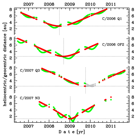
Figure 3: Comets with long time intervals of data arranged in order of decreasing $q_{\rm osc}$ (from top to bottom). Time distribution of positional observations with corresponding heliocentric (red curve) and geocentric (green curve) distance at which they were taken. Horizontal dotted lines show the perihelion distance for a given comet whereas vertical dotted lines – the moment of perihelion passage. The horizontal axis for all panels is exactly the same. For Comet C/2007 Q3 time interval, where the O-C diagrams give significant trends in right ascension and declination (remains visible even in a NG model) is shown in light gray – this period correlates with the moment when a secondary fragment broke away from the nucleus.

One can see in Fig. 3 that all four comets of this group have been observed more than three years in a broad range of heliocentric distances from at least 6 au before the perihelion passage to over 6 au after perihelion. Thus, long time sequences of data should allow us to model the NG orbital motion in great details. In particular, these should allow for examining various forms of $g(r)$-like function (Paper 3).

In fact, long time series of data allow us to determine the NG effects of all these comets basing on the entire ranges of data, and all their NG orbits are of the highest accuracy (1a+ class, see Table 1). In all cases where we were able to apply an asymmetric NG model relative to the moment of perihelion passage (Section 2.1), such a model however did not show any decrease in rms in comparison to a symmetric NG model (Table 2) and did not give a better similarity of O-C distribution to a normal distribution and/or better O-C diagram. Moreover, it was not possible to derive any dedicated form of $g(r)$-like functions for these comets. We were also not able to formulate any concrete conclusions about the potential deviation of value of the exponent $m$ in Eq. 4 from the standard value $m_{\rm STD}=-2.15$, or about the different value of scale distance than the standard $r_{0}=2.808$ au (Eq. 2).

C/2006 OF₂ Broughton

NG models of this comet provide O-C distributions very good approximated by Gaussian distribution and give very reasonable values of NG parameters with dominant and positive radial component of NG acceleration and negligible normal component in comparison to the remaining two $A_{1}$ and $A_{2}$ components (Table 2). However, even assuming $A_{3}=0$, the tau-shift can not be determined (its value oscillates with large amplitude around more than 100 days before perihelion). Due to some slight trends in the O-C diagram we added the gravitational PRE model as an alternative for studying past dynamics of this object.

C/2006 Q1 McNaught

Here, NG models result in O-C distributions good approximated by Gaussian distribution and no trends in O-C-diagram was noticed. The normal component of NG motion in the standard MSY model seems to be important in orbital fitting and gives a significantly decrease of rms in comparison to model with two NG parameters (radial and transverse components) as well as in model including also $\tau$-shift of $g(r)$-function and ignoring normal component (Table 2). We added the gravitational PRE model as an alternative for studying past dynamics of this object – just for comparison.

C/2007 N3 Lulin

This comet has the smallest perihelion distance in this group, $q_{\rm osc}=1.21$ au. Therefore, starting this investigation we suspected that we would get some interesting information about $g(r)$-like function for this comet. Unfortunately, models based on individually adjusted $g(r)$-like function did not give noticeably better fitting to observations.

For NG model with three components of NG accelerations the significant decrease of rms was noticed from 0$.\!\!^{\prime\prime}$50 to 0$.\!\!^{\prime\prime}$35. It can be seen (Table 2) that values of three NG parameters, $A_{1},A_{2},A_{3}$, although small, are well-defined, however A3 component slightly dominates over $A_{1}$ and $A_{2}$. Asymmetric model with two components of NG accelerations and tau ($A_{1}+A_{2}+\tau$) gives the rms of 0$.\!\!^{\prime\prime}$49 (significantly greater than symmetric model with $A_{3}$) Asymmetric model with four parameters ($A_{1}+A_{2}+A_{3}+\tau$) gives rms of 0$.\!\!^{\prime\prime}$35, thus indistinguishable from the symmetric model with three parameters ($A_{1}+A_{2}+A_{3}$, see Table 2).

Moreover, all considered NG models based on the entire interval of observations give the O-C distribution that substantially differs from a normal distribution. For that reason we would recommend gravitational models PRE and POST instead, especially for studying past and future dynamics of this object.

NG solution based on entire data set as well PRE (POST) type of solution give very similar values of $1/a_{\rm ori}$ ($1/a_{\rm fut}$). Thus, past and future dynamics of this comet seems to be very well defined.

C/2007 Q3 Siding Spring

This comet must be examined in a special way. In the middle of March 2010, Nick Howes reported a small secondary piece of C/2007 Q3 on the picture taken using Faulkes Telescope North. The existence of this secondary component was later confirmed during the follow-up observations taken from Mar. 17 up to Apr. 9 by many other observers (Colas et al., 2010). Indeed, this period correlates with a time interval where significant trends in both right ascension and in declination appear in the O-C diagrams even in the NG model of motion (light grey part of data in the third panel from the top of Fig. 3). GR orbit of C/2007 Q3 based only on pre-perihelion data is still 1a+ quality class.

Maybe due to this additional event, the NG model of C/2007 Q3 based on entire data interval gives radial component, $A_{1}$, smaller than the other two components $A_{2}$ and $A_{3}$ (Table 2). Similarly as in C/2007 N3 we noticed here important role of a normal component of NG acceleration in rms decreasing.

Similarly as in remaining comets in this group, the NG solution based on entire data set as well PRE (POST) type of solution give similar values of $1/a_{\rm ori}$ ($1/a_{\rm fut}$). Thus, past and future dynamics also for this comet seems be well-defined.

4.2 Group B: peculiar comets

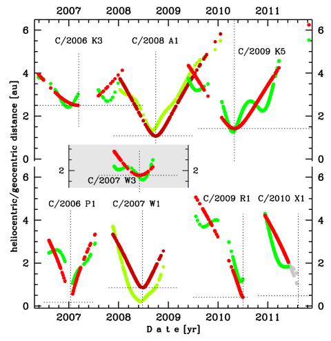
Figure 4: The same as in Fig. 3 for peculiar comets. The horizontal axis is common for all comets and is the same as in Fig.  3. The vertical scale unit is also the same as in the previous figure. Four comets with perihelion distances, $q_{\rm osc}$, below 1.0 au are shown in the bottom part of this figure.

We found that eight comets in the studied sample exhibit some kind of unusual activity or are troublesome in determining the osculating orbit. All of them we classified as peculiar objects and discussed in this section.

In the bottom part of Fig. 4 the positional measurements for four comets with the smallest perihelion distances in our sample are shown: C/2006 P1, C/2009 R1, C/2010 X1 and C/2007 W1.

Among the remaining four comets in this group we have C/2008 A1 with strong and variable NG effects in its motion, two more comets with NG effects clearly seen in the motion and easily determinable from the entire interval of data (C/2007 W3 and C/2006 K3), and C/2009 K5, whose osculating orbit was especially difficult to determine (see below).

Table 6: NG parameters derived in the present investigation and by Nakano (Nakano, 2009a, b, c) for two comets with strongly manifesting NG effects in the motion.

Source	NG model	$A_{1}$		$A_{2}$		$A_{3}$		No of	rms	interval of data
		NG parameters (Eq. 2) in units of $10^{-8}$						obs.	′′	[yyyymmdd]
$[1]$	$[2]$	$[3]$		$[4]$		$[5]$		$[6]$	$[7]$	$[8]$
C o m e t      C/2007 W1    B o a t t i n i
present	PRE	1.002 $\pm$	0.139	-0.7253 $\pm$	0.0032	-0.4916 $\pm$	0.0703	926	0.49	20071120–20080612
	POST	5.866 $\pm$	0.272	-0.783 $\pm$	0.172	0.138 $\pm$	0.250	777	0.59	20080630–20081217
NK1731A	PRE	1.905 $\pm$	0.072	-0.5243 $\pm$	0.0302	–		804	0.57	20071120–20080612
NK1731B	POST	5.753 $\pm$	0.111	-0.705 $\pm$	0.150	–		733	0.63	20080630–20081107
C o m e t      C/2008 A1    M c N a u g h t
present	NG	5.150 $\pm$	0.032	0.9915 $\pm$	0.0201	0.1939 $\pm$	0.0076	997	0.44	20080110–20100117
	PRE	4.608 $\pm$	0.136	1.894 $\pm$	0.233	1.844 $\pm$	0.203	393	0.28	20080110–20080928
	POST	10.094 $\pm$	0.282	6.142 $\pm$	0.291	-4.431 $\pm$	0.306	544	0.54	20081001–20100117
NK1807	NG	5.099 $\pm$	0.047	0.7641 $\pm$	0.0272	–		869	0.71	20080110–20090714

Comets C/2007 W1 (1.2 yr of data) and C/2008 A1 (2 yr) exhibit the most manifesting NG effects in their motion among comets studied in this paper. NG models based on the entire set of positional data proved to be completely inappropriate for both these objects; the detailed discussion of NG models based on full data sets was given in Section 2.2. Moreover, NG effects appear to be variable inside the interval covered by positional data. Such an erratic behaviour can be detected by using data taken before perihelion passage and after perihelion to determine the set of NG parameters, separately for both orbital branches. The results are given in Table 6, where also the NG parameters derived by Nakano (2009a, b, c) are shown. One can see that our values of NG parameters are in very good agreement with Nakano though he assumed that $A_{3}=0$ and used slightly different sets of data. Unfortunately, Nakano analysed NG effects for pre-perihelion and post-perihelion data separately only for C/2007 W1, so solely solutions for this comet could be compared in Table 6.

C/2006 K3 McNaught

NG effects easily determinable from the entire interval of data despite a moderate perihelion distance of 2.5 au. The radial component of NG acceleration dominates and is well-determined, we decided to include the normal component to the model since this gives slight improvements in rms and O-C-diagram and generalize the NG solution; no other tailored model is needed for this object.

C/2006 P1 McNaught

This comet ($q_{\rm osc}=0.17$ au) was the second brightest comet observed by ground-based observers since 1935 and demonstrated a spectacularly structured huge dust tail (e.g. Jones et al., 2008). It might be surprising that in case of such an active comet with extremely small perihelion distance it was possible to obtain a very well determined, standard NG orbit from the whole data set. Best NG solution is based on radial and transverse components of NG acceleration.

C/2007 W1 Boattini

This comet is also discussed at the beginning of this section together with comet C/2008 A1. We detected strong and variable NG effects in its motion. As a result we recommend separate, nongravitational PRE and POST models for studies of its past and future dynamics. The similar approach was proposed by Nakano, see Table  6 for more details. Our all osculating orbit solutions (Section 2.1, Tables 2-3) show that C/2007 W1 ($q_{\rm osc}=0.85$ au) , having a negative value of $1/a_{\rm ori}$ is an excellent candidate to be an interstellar comet. It is therefore important at this moment to refer to two quite different publications on this comet. In the first, Villanueva et al. (2011) measured a chemical composition of C/2007 W1 using NIRSPEC at Keck-2. They derived the abundance ratios of eleven volatile species relative to the water and concluded that almost all these ratios are among the highest ever detected in comets (see figure 8 therein). Thus, this comet seems to be very peculiar also in the light of chemical composition.

In the second paper interesting from our point of view, Wiegert et al. (2011) reported a new daytime meteor shower detected using Canadian Meteor Orbit Radar. They analysed the data in the 2002-2009 interval and detected Daytime Craterid shower in two years: in 2003 and 2008. Next, they concluded that this shower can be connected with C/2007 W1 because of the similarity of both sets of orbital elements, excluding eccentricities. They argued that the eccentricity of C/2007 W1 is known with so great uncertainty that this comet can be a short-period comet giving two showers. According to the authors, the second shower detected in 2008 would be after C/2007 W1 perihelion passage in 2007, the first one – at the previous perihelion passage of this comet. In our opinion, however, the orbit of this comet is known much more accurately than Wiegert et al. (2011) argued. Thus, only the shower in 2008 could be related to C/2007 W1.

C/2007 W3 LINEAR

NG effects clearly seen in the motion of this comet and the standard NG model is easily determinable from the entire interval of data. The asymmetric model is marginally determinable, however with large uncertainties of $\tau$-shift and with no improvements of orbital fitting (Table 2). No other tailored model is necessary to represent the positional data of this object.

C/2008 A1 McNaught

This comet is also discussed at the beginning of this section together with comet C/2007 W1. Due to the nature of the detected NG forces (strong and variable) we recommend separate, nongravitational PRE and POST models for studies of its past and future dynamics. For comparison we show also two models based on the entire data set: an asymmetric one and a standard, symmetric model.

C/2009 K5 McNaught

This comet also seems to be a peculiar object. Considering rather long time interval of observations (2.5 yr) it could be optionally included into the group of comets with long sequences of data since its observations cover quite large heliocentric distances from 4.35 au before perihelion to 6.25 au after perihelion (orbit 1a+ class). This fact, together with small perihelion distance, should create a perfect opportunity to determine the NG effects either from the whole data set (as for all comets of long data sets in this paper, previous subsection) or from pre-perihelion and post-perihelion data individually, as in the case of C/2007 W1 or C/2008 A1. In contrast to the expectation, the NG effects cannot be reliably determined from the entire data set of C/2009 K5 as well as individually from pre- or post- perihelion orbit branches. Thus, we decided to include this comet to peculiar objects. We recommend separate gravitational PRE and POST models for this comet and present two other models for comparison.

C/2009 R1 McNaught

This comet of a very small perihelion distance ($q_{\rm osc}=0.405$ au) was observed only prior to its perihelion passage and was lost soon after it. There is no information about this comet after perihelion and we can speculate that this comet has disintegrated. Among comets observed only before perihelion passage C/2009 R1 exhibits strong and well-determinable NG effects during interval covered by positional measurements and belongs to comets with good quality NG orbit (see also Fig. 1).

C/2010 X1 Elenin

Another peculiar comet of a very small perihelion distance ($q_{\rm osc}=0.482$ au). It starts to disintegrate about one month before perihelion and it turn out that only a pure gravitational orbit can be well determined from the shorter interval of data – the part of data not included in the orbit determination is shown in light grey in Fig. 4. On the occasion of this comet, it is worth mentioning that even when a cometary disintegration was observed, some authors derived NG orbit with standard (constant!) NG parameters A₁, A₂, A₃, although they describe the systematic acceleration acting on a comet, which is a function of the heliocentric distance from the Sun. These standard NG parameters cannot correctly account for a sudden change in orbital motion due to comet’s partial disruption. Therefore, the interpretation of results obtained in such a case should be restricted to the statement that some NG effects are clearly seen in the cometary motion but nothing more. It seems to us that the values of orbital elements in such a NG case also should be treated with great caution. Comet C/2010 X1 just may be an good example of such a case of misusing the standard MSY method.

4.3 Group C: comets of non-detectable or very weak NG effects

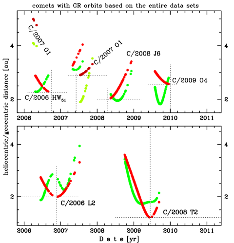
Figure 5: The same as in Fig. 3 for comets of non-detectable or very weak NG effects. The horizontal axes covers exactly the same time-interval in both panels and the same time-scale was used as in Fig. 3.

Whether NG effects are noticeable in comet’s motion or not depends on many factors such as quality and structure of data, the general level of activity and physical properties of comet (the nucleus structure, chemical composition, its shape and mass). Thus, generally each case should be individualized. However, it turns out that we often can pretty well predict whether it is possible to determine the NG orbit from the inspection of structure of the data, where by ’structure’ we mean here all that can be seen in the plot of the heliocentric and geocentric distances of all positional measurements.

It is rather not surprising that for three of six comets to be described in this section, namely for C/2007 O1 ($q_{{\rm osc}}=2.88$ au), C/2009 O4 ($q_{{\rm osc}}=2.56$ au) and C/2008 J6 ($q_{{\rm osc}}=2.00$ au) we do not succeed in determining NG effects in their orbital motion. We can expect this from quick inspection of Fig. 5.

In the remaining three cases, the situation is not as clear as above. From a review of Fig. 5 (notice that the scale of horizontal and vertical axes in both panels are the same) it is not obvious that NG effects are not detectable within time intervals covered by data. Of course, in this type of a qualitative discussion we assume some physical similarities between considered comets, mainly in their global activity.

In fact, for three comets described below, C/2006 HW₅₁, C/2006 L2 and C/2008 T2, we detected some traces of NG effects in positional data with a negative radial component of the NG acceleration (models marked as NG_A1 in column [2] of Table 3; see also discussion in Section 2.1). However, in all these cases we noticed only slight improvements in data fitting in comparison to GR orbit. Therefore, the interpretation of these NG models can be twofold. These models reflect the actual NG acceleration of these comets (for example giving some indication of the existence of active sources on the nucleus as was mention above), or the observed slight improvements in data fitting are only the result of a larger number of parameters taken into consideration when determining the NG orbit. We decided, however, to include these NG models to Table 3 solely as alternative models for dynamical status discussions based on the previous perihelion calculations, see Part II.

C/2006 HW₅₁ Siding Spring

The data structure of this comet is qualitatively quite similar to that of comet C/2006 K3, a number of measurements is also very similar (about 200 observations in both cases). Furthermore, both comets passed perihelion rather far from the Sun (more than 2.2 au). It seems, however, that the longer time interval of data (1.7 years), resulting in a wider range of observed heliocentric distances before perihelion in the case of C/2006 K3 (3.95 au at the moment of discovery in comparison to 2.87 au at for C/2006 HW₅₁), causes that the NG acceleration in C/2006 K3 is clearly visible in its motion, while in the motion of comet C/2006 HW₅₁ it is not so easily discernible. The NG effects can be firmly detected in the motion of C/2006 K3 also due to the fact that this comet was significantly more active than C/2006 HW₅₁. One can speculate that the activity of the comet C/2006 HW₅₁ is limited only to some active areas somehow specifically located on the surface of the comet causing that standard MSY model gives some traces of NG effects with negative radial component of NG acceleration. We recommend pure gravitational model for this object, but we also present NG and gravitational PRE models for comparison.

C/2006 L2 McNaught

Similar arguments to the presented above seems to be correct in the case of comet C/2006 L2, that also passed through perihelion not very close to the Sun ($q_{\rm osc}=1.994$ au) and displays some traces of NG effects with negative $A_{1}$. We recommend pure gravitational model for this object, while NG and gravitational PRE models are presented for comparison.

C/2007 O1 LINEAR

In the data of C/2007 O1, we have more than one-year gap in positional measurements. This is due to the fact that the object was initially discovered as an asteroid, and more than a year later it was rediscovered as a comet. Data of such an unusual structure, where 12 observations were collected far before perihelion when the object was more than 4 au from the Sun and the rest of data were taken after the perihelion passage, together with the rather large perihelion distance, can effectively prevent the determination of NG effects despite quite a long period formally covered by measurements, so we present only pure gravitational solution for this comet.

C/2008 J6 Hill

Comet C/2008 J6 was followed from a heliocentric distance of 2.04 au to 3.43 au, thus in a wider range of heliocentric distances what is more promising. However, it was discovered after passing through the perihelion. In this case, the chance to detect the NG acceleration in the motion of even moderately active comet is low, only GR model is presented.

C/2008 T2 Cardinal

Comet C/2008 T2 seems to be a more unusual object. In terms of the structure of data we have a situation quite similar to that of comet C/2007 W3 (Fig. 4), but here we have much more measurements as well as the comet came closer to the Sun at perihelion (1.20 au compared to 1.78 au for C/2007 W3). Both facts should allow us to determine the NG effects easier for C/2008 T2 than for C/2007 W3. However, in this comet the NG effects are loosely detectable (almost at a noise level. One can suppose that comet C/2008 T2 probably exhibits another character of activity than C/2007 W3 or/and physically differs from C/2007 W3. We recommend GR model obtained from the entire dataset for this object, but we also present NG and gravitational PRE models for comparison.

C/2009 O4 Hill

Comet C/2009 O4 was observed only before perihelion passage in the narrow range of heliocentric distance from 3.04 au to 2.57 au and only during 4.5 months period, therefore only the gravitational model can be obtained.

4.4 Group D: comets of weak quality of osculating orbits

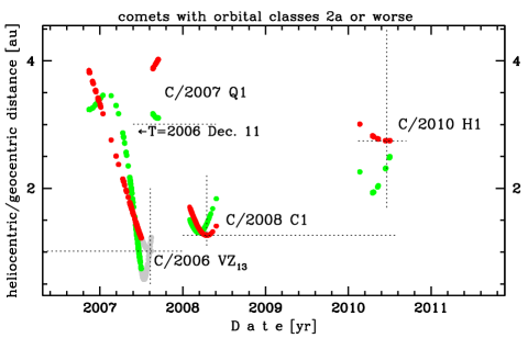
Figure 6: The same as in Fig. 3 for comets of weak quality of osculating orbits; also the same time-scale was used in horizontal axis. The time interval not taken for the determination of PRE type of osculating orbit of comet C/2006 VZ₁₃ is shown in light grey ink.

Due to a generally poor quality of osculating orbits of these four comets in comparison to others and their asymmetric distribution of observations relative to perihelion we should be very careful when making statements about their past and future motion. Moreover, we should admit that one of them (C/2006 VZ₁₃), split into separate fragments or disintegrated near perihelion.

C/2006 VZ₁₃ LINEAR

The observations of C/2006 VZ₁₃ ($q_{\rm osc}=1.01$ au, the smallest perihelion distance in this group) were stopped very soon after its perihelion passage. C/2006 VZ₁₃ (Fig.  6), was observed longer than remaining objects in this group, about eight months, while three others less than five months. However, it belongs to this group because in fact the only adequate orbit for its past dynamical evolution can be determined from the pre-perihelion data. We decided to cut the pre-perihelion string of data on July 1, 2007 ($1.23$ au from the Sun), i.e. 40 days prior to the perihelion passage because with such a restriction we derived the NG osculating orbit that gives O-C diagram free from any trends in right ascension or declination. For this reason the orbit based on this time interval is the most appropriate as starting orbit for the past dynamical evolution (see Part II of this investigation). The range of data that was not used for PRE type of model determination is shown in light grey ink in Fig.  6. Thus, the data time interval taken for the past evolutionary studies was only $\sim$7.5 months in this case. Shortening the time interval of data by almost 20 per cent resulted here in a more than four-fold reduction of a precision of $1/{\rm a}_{\rm osc}$-determination, and resulted in a decrease in its orbital class from 1b (NG orbit determined from the entire data set) to class 2a (NG orbit based on pre-perihelion data). For a future dynamical evolution we have no choice and for this purpose the NG orbit based on the entire data set was used. It is worth noting that the future orbit should be treated with great care because of our ignorance of the fate of this comet shortly after perihelion passage (the last observation was taken four days after perihelion).

C/2007 Q1 McNaught

This comet have the greatest perihelion distance ($q_{\rm osc}=3.01$ au) and the worst quality orbit (3a) in this group (and in the whole sample of comets examined in this paper) is determined for this comet.Its poor quality is a direct consequence of the shortest data arc throughout the sample (only 24 days) and also of an unusual moment of discovery, more than eight months after it passed through perihelion. Usually, when the astrometric observations include perihelion then the orbit have a chance to be more precisely determined. Only the pure gravitational orbit can be determined in this case.

C/2008 C1 Chen-Gao

Despite a very short time interval of data, the NG effects are detectable in the motion of this comet ($q_{\rm osc}=1.26$ au). However the NG parameters are not well determined and the decrease in rms is not observed, so we present the NG model for this comet only for comparison and recommend the GR model.

C/2010 H1 Garradd

It is impossible to detect the NG effects from the set of data for this comet due to very narrow data range – observations span a short time period. Additionally, we can notice that it passed the perihelion at the moderately large distances from the Sun ($q_{\rm osc}=2.745$ au), and only a small number of measurements were taken. As a result only a GR model can be obtained.

5 Original and future orbits

In the present numerical calculations, a dynamical evolution investigation of a given object starts from the swarm of VCs constructed using the osculating orbit (so-called nominal osculating orbit) determined in the respective model shown in Table 3. We performed dynamical calculations for each model presented in this table. Of course, for models based on PRE data we follow only the past evolution, whereas for models based on POST data – only the future evolution. Each individual swarm of starting osculating orbits is constructed according to a Monte Carlo method proposed by Sitarski (1998), where the entire swarm fulfil the Gaussian statistics of fitting to positional data used for a given osculating orbit determination. Similarly to our previous investigations (see for example Paper 1), each swarm consists of 5 001 VCs including the nominal orbit; we checked that the number of 5 000 orbital clones gives a sufficient sample for obtaining reliable statistics at each step of our study, including the end of our numerical calculations, i.e. at the previous and next perihelion passage (see Part II of this investigation). Therefore, we are able to determine the uncertainties of original and future reciprocal of semimajor axis ($1/a_{\rm ori}$ and $1/a_{\rm fut}$), that are here taken at 250 au from the Sun, i.e. where planetary perturbations are already completely negligible (Todorovic-Juchniewicz, 1981).

Values of $1/a_{\rm ori}$ and $1/a_{\rm fut}$ and their uncertainties derived by fitting the 1/a-distribution of original and future swarm of VCs to Gaussian distribution are given in columns $[9]$–$[10]$ of Table 3. All $1/a$-distributions as well as distributions of other orbital elements of analysed comets were still perfectly Gaussian at 250 au from the Sun. However, further evolution under the Galactic tides and stellar perturbation can potentially introduce significant deformations in the initially 6D-normal distribution of orbital elements in the swarms of VCs (up to 10D-normal distribution in the NG case), what will be shown in the Part II of this investigation.

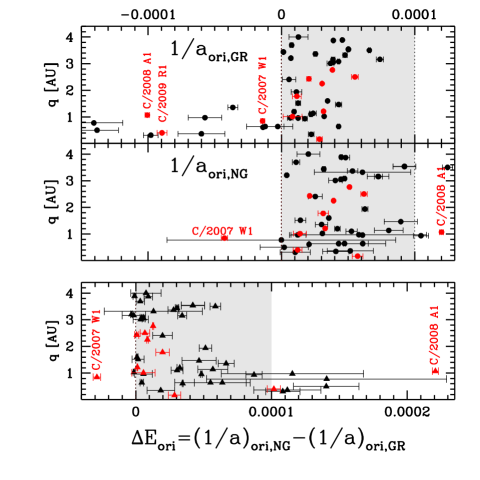
Figure 7: Shifts of $1/{\rm a}_{\rm ori}$ due to the NG acceleration for eleven comets from the period 2006-2010 (red symbols) with well-determined NG effects and 37 previously analysed comets (black symbols; Paper 1 & 2). Three largest uncertainties of $1/{\rm a}_{\rm ori,NG}$ belong to comets C/1959 Y1, C/1952 W1 and C/1892 Q1.

5.1 Original semimajor axes of NG orbits

First, it is important to notice that an osculating NG orbit determined from a given set of data is not the same orbit as one determined from these same observations but under the assumption of purely gravitational motion (Królikowska, 2001). Therefore, the change of original $1/a$-value due to incorporating the NG acceleration in the process of orbit determination can be even very large though the NG effects provide only modest changes in the original 1/a-value along an individual orbit. Typically, the original eccentricity of NG orbit are smaller than eccentricity of GR orbit for a given comet with determinable NG acceleration (where both GR and NG orbits are derived from the same set of positional data). We confirmed these general findings in the present studies. However, we found some interesting atypical behaviour for comet C/2007 W1.

The differences between the inverse original semimajor axes derived in NG model of motion and less realistic pure gravitational model of motion are presented for 11 comets examined here (red symbols) and 37 comets studied in the Paper1&2 (black symbols) in Fig. 7. In the bottom panel the dependence of the strength of NG forces on the osculating perihelion distance, $q_{\rm osc}$ is clearly visible for the whole set of 48 comets with determined NG effects.

To maintain consistency with previous our studies, the values of 1/a_ori and their uncertainties presented in this plot are based on osculating NG orbits determined from the entire data sets except of the comet C/2007 W1 where we took the value of 1/a_ori determined from the NG orbit based on pre-perihelion subset of data as significantly more adequate for this comet (see also Section 4.2). Nakano (2009a, b) also considered the pre-perihelion and post-perihelion orbital branches independently for this particular comet. He derived a similar value of 1/a${}_{\rm ori}=-0.000059$ au^-1 on the basis of pre-perihelion data only (the detailed comparison of both NG models is given in Section 4.2. However, for the NG orbit based on the entire observational interval we obtained even a more negative value of 1/a${}_{\rm ori}=-0.000082\pm 0.000003$ au^-1. Thus, C/2007 W1 Boattini is the first serious candidate for interstellar comet among LPCs examined by us so far.

Table 7: Three samples of comets with $1/a_{\rm ori}<10^{-4}$ au^-1: qS, qM and qL in comparison to MWC 08. The number of comets are given for first quality class orbits in MWC 08, except the sample of comets investigated in this paper, where 3 objects with quality class 2 and 3 are included; we indicate this by ’$+$ 3’ in columns [3] & [9].

	N u m b e r    o f    c o m e t s    i n    t h e    d i f f e r e n t    s a m p l e s
Period	$q_{{\rm osc}}<3.1$ au		$3.1\leq q_{{\rm osc}}<5.2$ au		$q_{{\rm osc}}\geq 5.2$ au		All comets
of discovery	MWC 08	Sample qS	MWC 08	Sample qM	MWC 08	Sample qL	MWC 08	analysed by us
$[1]$	$[2]$	$[3]$	$[4]$	$[5]$	$[6]$	$[7]$	$[8]$	$[9]$
before 1900	10	2	–	–	–	–	10	2
1900–1949	26	3	6	–	–	–	32	3
1950–1999	24	16	22	17	11	11	57	44
2000–2005	10	6	14	14	12	11	36	31
2006–2010	12	19 $+$ 3	3	4	3	2	18	25
All	82	46 $+$ 3	45	35	26	24	153	105 $+$ 3

In the case of comet C/2008 A1 we show in Fig. 7 the results based on the entire data interval though for this comet the NG orbit determined from the full interval is also highly unsatisfactory (as we discuss earlier). The largest differences in $\Delta{\rm E}_{\rm ori}$ was derived just for this comet (the rightmost red symbol in the bottom panel of Fig.7), whereas based on a pre-perihelion subset of data we derived 1/a${}_{\rm ori}=0.000120\pm 0.000002$ au^-1 for NG orbit and $\Delta{\rm E}_{\rm ori}=-0.000011$ au^-1. However, we would like to stress that C/2008 A1 as well as C/2007 W1 are comets that both have extremely strongly manifesting and variable NG effects inside their observational intervals.

Sets of original and future 1/a-values taken for statistical analysis (see next section) are based on the preferred osculating orbits. It is obvious that NG orbits – if determinable in the motion of a given comet – are always more realistic than pure gravitational orbit derived from the same data set.

5.2 Observed distributions of original and future semimajor axes

In the discussion below we do not pretend to describe planetary perturbations on LPCs in general. Instead, we aim to present really observed changes in $1/a$ for a significant percentage of the observed LPCs, additionally for the first time fully accounting for their uncertainties. We also discuss the contribution of the NG forces into the $1/a$ change during a cometary flyby through the planetary system.

To describe the original and future $1/a$-distributions we divided 108 comets investigated by us so far (in the present investigation and Papers 1 & 2) into three subsamples of a different completeness according to their osculating perihelion distances:

qS

– this sample consists of 49 LPCs with $q_{\rm osc}<3.1$ au and includes comets with strongly manifesting NG effects in their motion discovered before 2006 (Papers 1 & 2) and a complete sample of comets discovered in the period 2006-2010 investigated in this work. Thus, we have here 46 of 89 (52 per cent) comets discovered before 2011 with first quality class orbit by using original MSE method (Section 3) and additionally three comets of poorer quality class orbits.

qM

– complete sample of 35 LPCs with 3.1 au $\leq q_{\rm osc}<5.2$ au discovered in the period 1970-2006 (first quality class orbits, Paper 2).

qL

– almost complete sample of 24 LPCs with $q_{\rm osc}\geq 5.2$ au discovered before 2008 (first quality class orbits, Paper 2); only two objects, C/2005 L3 and C/2007 D1, were not taken into account in Paper 2 because they were still observable at the beginning of 2012.

Table 8: Contribution of planetary perturbations and NG effects to $\delta(1/a)=1/a_{\rm fut}-1/a_{\rm ori}$ for nine comets with NG orbits given as the preferred models of their motion in Table 3. Comets are arranged in order of increasing $q_{\rm osc}$. In the first row of individual comet $\delta(1/a)$ for the main NG model (given in the first rows in Table 3) is presented, the second row shows $\delta(1/a)$ obtained using the best GR model and third row displays the $\delta(1/a)$ derived using the same NG orbit as in the first row, however during integration backward and forward to the 250 au from the Sun the NG acceleration was excluded. In the second row (column $[9]$) the percentage change in $\delta(1/a)$ relative to first row is also given. Values of $1/a_{\rm ori}$, $1/a_{\rm fut}$, and $\delta(1/a)$ are given in units of $10^{-6}$ au^-1 used in this paper, and the magnitude of the NG acceleration, $A=\sqrt{A_{1}^{2}+A_{2}^{2}+A_{3}^{2}}$, in units of $10^{-8}$ au$\cdot$day^-2.

Comet	$q_{{\rm osc}}$	type of	Model of	rms	$1/a_{{\rm ori}}$	Model of	$1/a_{{\rm fut}}$	$\delta(1/a)$	N G   p a r a m e t e r s
	[au]	motion	orbit for	for $[4]$		orbit for			pre-perihelion		post-perihelion
			$1/a_{{\rm ori}}$	′′		$1/a_{{\rm fut}}$			$A$	$A_{2}/A_{1}$	$A$	$A_{2}/A_{1}$
$[1]$	$[2]$	$[3]$	$[4]$	$[5]$	$[6]$	$[7]$	$[8]$	$[9]$	$[10]$	$[11]$	$[12]$	$[13]$
C/2006 P1	0.171	NG	NG	0.25	57.2	NG	467.6	410.5	1.33	0.23	1.33	0.23
		GR	GR	0.25	31.4	GR	490.7	459.3 (11.4%)
		GR	NG	0.79	37.4	NG	496.7	459.3
C/2009 R1	0.405	NG	NG	0.51	12.2	NG	170.4	158.3	6.02	0.24	6.02	0.24
		GR	GR	0.63	-89.6	GR	-723.0	-812.6
		GR	NG	4.87	12.2	NG	-592.4	-551.7
C/2007 W1	0.850	NG	PRE,NG	0.49	-42.7	POST,NG	554.4	586.5	1.33	0.72	5.92	0.13
		GR	PRE,GR	0.61	-14.1	POST,GR	892.0	632.9 (7.9%)
		GR	PRE,NG	4.50	71.8	POST,NG	716.5	634.0
C/2006 VZ13	1.015	NG	PRE,NG	0.39	14.0	NG	491.2	269.3	2.13	0.46	5.63	0.66
		GR	GR	0.40	13.6	GR	442.2	435.6 (62%)
		GR	PRE,NG	5.31	132.8	NG	371.2	30.4
C/2008 A1	1.073	NG	PRE,NG	0.28	120.8	POST,NG	246.5	-534.1	4.98	0.41	12.62	0.61
		GR	PRE,GR	0.47	132.4	POST,GR	258.4	268.9
		GR	PRE,NG	14.11	137.6	POST,NG	1065.05	267.6
C/2007 W3	1.776	NG	NG	0.52	31.4	NG	343.9	312.5	5.56	0.45	5.56	0.45
		GR	GR	0.54	14.2	GR	408.8	394.6 (26.3%)
		GR	NG	3.70	21.2	NG	415.8	394.6
C/2006 OF2	2.431	NG	NG	0.36	21.2	NG	-658.8	-680.0	2.75	0.58	2.75	0.58
		GR	GR	0.38	23.7	GR	-662.4	-686.1 (0.9%)
		GR	NG	0.49	24.9	NG	-661.1	-686.1
C/2006 K3	2.501	NG	NG	0.54	61.0	NG	-131.3	-192.3	15.85	0.14	15.85	0.14
		GR	GR	0.69	61.9	GR	-123.0	-184.9 (3.9%)
		GR	NG	1.19	62.0	NG	-122.9	-184.9
C/2006 Q1	2.764	NG	NG	0.37	51.1	NG	707.4	656.4	35.19	0.06	35.19	0.06
		GR	GR	0.50	38.3	GR	696.6	658.3 (0.3%)
		GR	NG	2.05	52.7	NG	711.0	658.3

More detailed descriptions of these three samples are given in Table 7 where the completeness of these samples in comparison to MWC 08 is shown. MWC 08 is complete to the end of the 2007. In the period of 2006–2010, considerable number of 48 LPCs with $1/a_{\rm ori}<10^{-4}$ au^-1 were discovered (eight of them are still observable), and all of them, having $q_{\rm osc}<3.1$ au are investigated in this paper and are shown by red points in Fig. 8. In total, our sample of 108 comets discussed here constitutes more than 60 per cent of all first class Oort spike comets discovered after 1800 (78 per cent of those discovered after 1950), for which observations are finished. For the present discussion only the preferred models (shown in the first row for each comet in Table 3) were taken into consideration.

In a pure GR model of cometary motion, the values of $\delta(1/a)=1/a_{\rm fut}-1/a_{\rm ori}$ directly inform about planetary perturbation which a comet suffered passing through the planetary system. When the NG osculating orbit is derived we should expect that NG effects contribute in some extent to the value of $\delta(1/a)$. It is not so easy to measure these contributions, in particular for these comets where two separate NG osculating orbits are preferred to describe their actual orbital motion. We have made such an attempt in the case of comets with NG orbits investigated here.

Table 8 presents three values of $\delta(1/a)$ for all comets with NG models chosen by us as the preferred solution in Table 3. For each comet, the first row gives $\delta(1/a)$-value for the recommended NG model, the second row – $\delta(1/a)$-value for the best GR model, whereas the third row shows $\delta(1/a)$-value derived for the same NG osculating orbit taken as a starting orbit, however NG accelerations were not included during the integration backward and forward to 250 au from the Sun for original and future 1/a-determination. Of course, the last orbit does not represent data (see column $[5]$) since the best GR orbit that gives good data fitting (second row, column $[4]$) is substantially different than the best NG orbit. However, the difference between first row and second (and third) row may give some estimation for the NG contribution to the $\delta(1/a)$-value. For comets with separate NG orbits derived for pre-perihelion branch and post-perihelion branch, we calculate the $\delta(1/a)$ from the equation:

$$\delta(1/a)=(1/a_{\rm fut}-1/a_{\rm osc,post})-(1/a_{\rm ori}-1/a_{\rm osc,pre}),$$

where $1/a_{\rm osc,post}$ and $1/a_{\rm osc,pre}$ are values of $1/a_{\rm osc}$ for post-perihelion and pre-perihelion orbit, respectively.

One can notice using Table 8 that for comets with perihelion distance greater than 2.0 au the $\delta(1/a)$-value can be interpreted as planetary perturbations even in the NG models of motion. We have also confirmed this conclusion for all comets studied in Paper 1 & 2 where differences in $\delta(1/a)$-value between NG and GR models do not exceed 10 per cent, except C/1997 J2 where we obtained this difference at the level of 40 per cent due to a very small value of $\delta(1/a)$ ($-41$ and $-30$ for GR and NG orbit, respectively). However, for smaller perihelion distances ($q_{\rm osc}<2.0$ au) we can obtain even a change of sign of $\delta(1/a)$, like for C/2009 R1 ($q_{\rm osc}=0.405$ au) and C/2008 A1 ($q_{\rm osc}=1.07$ au) with the highest magnitude of NG acceleration (columns $[10]$–$[13]$ in Table 8). Differences of more than 30 per cent in $\delta(1/a)$ between NG and GR models are found only for three comets investigated here (two peculiar comets, C/2008 A1 and C/2009 R1, and one of weak quality of osculating orbit, C/2006 VZ₁₃) and five comets of 37 with NG orbits determined in Papers 1 & 2. In the following discussion, when we use the term ’planetary perturbation’, we keep in mind that identification of planetary perturbation with $\delta(1/a)=1/a_{\rm fut}-1/a_{\rm ori}$ in the case of NG orbit is subject to an additional contribution, that exceed 30 per cent of $\delta(1/a)$-value just for a few of them. This contribution is obviously caused by slightly different evolution of orbital elements due to NG acceleration along a given orbit.

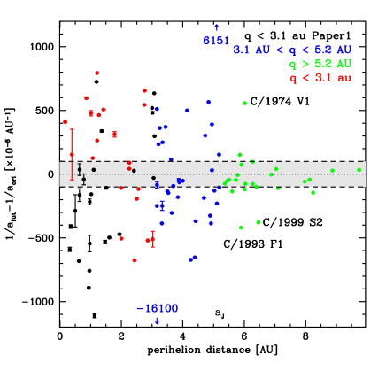
Figure 8: Change of reciprocals of semimajor axis during passage through the planetary zone, $\delta(1/a)=1/a_{\rm fut}-1/a_{\rm ori}$, as a function of osculating perihelion distance, where the sample of 22 comets investigated in this paper are shown by red dots. The sample of 86 comets studied in Paper1&2 were divided into three subsamples qS, qM and qL (see Table 7) and are given as black, blue and green dots, respectively. The vertical line marks the position of Jupiter semimajor axis at 5.2 au. The horizontal grey band between two horizontal dashed lines shows the area where planetary perturbations are smaller than $10^{-4}$ au^-1.

In Fig. 8 we show $\delta(1/a)=1/a_{\rm fut}-1/a_{\rm ori}$, in a function of osculating perihelion distance for the sample of 22 comets investigated here (red points) in comparison with all remaining 86 comets investigated by us so far. The uncertainties of $\delta(1/a)$ were derived by calculating the $\delta(1/a_{i})$ where $i=1,...,5001$ for each VC in the swarms, and then fitting the derived $\delta(1/a)$-distribution of individual swarm of VCs to Gaussian distribution. The uncertainties of perihelion distance and inclination are significantly below the size of points in these figures. It is interesting to notice that the largest $\delta(1/a)$-uncertainty in the group of comets investigated in the present paper and in the entire sample of 108 Oort spike comets, were obtained for C/2009 R1 McNaught (orbital class: 1b), easy recognizable red point with largest vertical error bar. For C/2009 R1 we have $\delta(1/a)=154\pm 199$ in units used in this paper. At a first glance, this comet with large inclination to ecliptic ($\sim 77$^∘) seems to suffer a relatively moderate planetary perturbations (NG model). However, we found that the nominal VC have passed about 1.3 au from Jupiter in 2009 (on August 25), and 0.15 au from Mercury in July 2010 (six days after perihelion passage, the last observation of this comet was taken 10 days earlier).

Among the sample of comets from the 2006–2010 period, the second comet with large error of $\delta(1/a)$ is C/2007 Q1 Garradd ($\delta(1/a)=-510\pm 62$), however, this resulted from the extremely poor quality of its orbit (class 3a).

Apart from three comets (C/1940 R2, C/1980 E1 and C/2002 A3) lying outside Fig. 8 all other suffer only moderate perturbations in $1/a$, with a significant per cent of very small values (points inside the horizontal band around zero in the figure), conversely to widely spread opinion, that comets coming closer to the Sun than Jupiter almost certainly suffer strong planetary perturbations. It means, that in the sample of analysed Oort spike comets the number of objects that have a chance for returning in the next perihelion passage as an Oort spike comet is remarkable (see middle panels in Fig. 9) and accounts to about 14 per cent of all investigated by us near-parabolic comets (108 objects). This shows the observed transparency of the Solar system (see Dybczyński, 2004). This transparency seems to be significantly different for large perihelion near-parabolic comets than for small perihelion comets and, taking into account small number statistics fluctuations it is consistent with the results of the Monte Carlo simulations of this phenomenon, recently published by Fouchard et al. (2013). The detailed percentages of comets with $1/a_{\rm fut}$ still smaller than $100\times 10^{-6}$ au^-1 within three discussed samples are as follows:

qS sample	10 per cent
qM sample	6 per cent
qL sample	33 per cent.

This feature of the $1/a_{\rm fut}$ distribution is also clearly visible in Fig. 8, where the distributions of $\delta(1/a)$ as well as the distributions of $1/a_{\rm ori}$ and $1/a_{\rm fut}$ are presented in Fig. 9 in the bottom, top and middle panels, respectively. The filled light steel-blue histograms show the distributions of 22 comets investigated in this paper. These steel-blue histograms, are overprinted on the blue histograms that represent qS sample (49 comets). Similarly, the distributions of comets of $q_{\rm osc}\geq 5.2$ au (filled light turquoise histograms, 24 objects) are overprinted on the distributions of qM$+$qL sample of comets (filled green histograms, 59 objects of $q_{\rm osc}\geq 3.1$ au). It should be stressed here that the uncertainties of $1/a_{\rm ori}$, $1/a_{\rm fut}$ and $\delta(1/a)$ are taken into account in these histograms by considering full cloud of 5001 virtual orbits for each comet. For example, the global distribution of $1/a_{\rm ori}$ in both upper panels (marked by thick black ink) is based on all clouds of VCs of 108 comets, thus in total of 540 108 VCs, whereas the global distributions of $1/a_{\rm fut}$ and $\delta(1/a)$ are based on 107 cometary swarms (in total of 535 107 VCs) where C/2010 X1 was not taken into account for future distribution because of its disruption during perihelion passage. One can see that a prominent maximum of the observed planetary perturbation is visible only for comets with $q_{\rm osc}\geq 3.1$ au whereas for qS sample of comets the distribution of planetary perturbation is broad with no sharp peak.

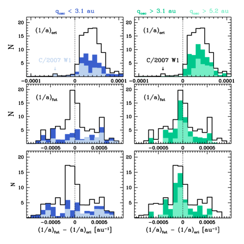
Figure 9: Distribution of $1/a_{\rm ori}$ (top panels), $1/a_{\rm fut}$ (middle panels) and $\delta(1/a)$ for small perihelion ($q_{\rm osc}<3.1$ au, left-side filled histograms) and large perihelion ($q_{\rm osc}\geq 3.1$ au, right-side filled histograms) Oort spike comets. The histogram given in each panel in thick black ink always represents the distribution of the whole sample of 108 comets. The uncertainties of $1/a$-determinations were incorporated into these $1/a$-histograms by taking the full cloud of VCs for each comet. The light steel-blue histograms in the left-side panels show the sample of 22 comets investigated in this paper, where the light turquoise histograms in the right-side panels represent the sample of comets with $q_{\rm osc}\geq 5.2$ au. Completeness of all samples are shown in Table 7.

There is another interesting feature visible in Fig. 9. The secondary peak between $0.0005$ au^-1 and $0.0006$ au^-1 is present in the distributions of $1/a_{\rm fut}$ that is visible in the qS sample as well as in the sample of comets with $q_{\rm osc}\geq 3.1$. This corresponds to the local maximum between 1 700 au and 2 000 au for the future semimajor axes. Outside the value of $0.0006$ au^-1 we observe significant and fast decrease in the $1/a_{\rm fut}$-distribution. It is interesting that the similar trend of decrease is observed around $0.0006$ au^-1 in the $1/a_{\rm ori}$-distribution for the sample of near-parabolic comets in MWC 08 (of first quality orbits).

We noticed that the investigated here sample of small perihelion Oort spike comets differs from the sample of small perihelion comets with strongly manifesting NG effects investigated in Paper 1 in the context of future history of these objects. Then, we derived that 60 per cent of them will be lost on hyperbolic orbits in the future, here we have only 33 per cent of such comets (seven objects escaping on hyperbolic trajectories and one object that disintegrated at perihelion). Taking into account all Oort spike comets with small perihelion distances investigated by us so far (49 objects) we have now 49 per cent of comets escaping in the future from Solar system on hyperbolas whereas for the whole sample of comets – the similar value of 53 per cent. Thus, the small perihelion cometary sample and the large perihelion sample appear to be quite similar in this regard. However, more comets, especially these with $q_{{\rm osc}}<3.1$ au need to be analysed with the NG effects taken into account. In the Part II we will discuss the differences between both samples in the context of dynamical status of near-parabolic comets.

6 Summary

We showed that the individualized approach to the osculating orbit determination is advisable, especially for the purpose of past and future dynamical evolution of near-parabolic comets. Developing such an attempt we have determined the osculating orbits for a complete sample of so-called Oort spike comets with a small perihelion distance ($q_{\rm osc}<3.1$ au) discovered in five year period from 2006 to 2010. For eleven of these comets (50 per cent) we detected NG effects in their orbital behaviour using entire sets of data (Table 1) and discussed various NG models (Table 2). The detailed investigation shows, however, that in five of them even more individualized approach is necessary (Table 3). Thus, we determined osculating orbits for pre-perihelion and post-perihelion orbital branch, separately. We argued that the separate NG solutions for each orbital leg for two of them, C/2007 W1 and C/2008 A1, are more adequate for past and future orbital evolution. Our solutions for both comets are very similar to solutions previously obtained by Nakano (Section 4.2). Additionally, for C/2006 VZ₁₃ the NG solution based on pre-perihelion orbital leg is presented. For the remaining two comets with NG effects detectable in the entire (very long) data sets, C/2007 N3 and C/2007 Q3, we proposed GR orbits derived from a pre-perihelion and post-perihelion branch as the best osculating orbit for past and future evolutionary calculations, respectively. Unfortunately, the NG effects were indeterminable for the pre-perihelion and post-perihelion leg separately in both comets despite long-time series of data.

Next, we discuss the possibility of NG acceleration detection in the motion of near-parabolic comets in the light of data location along their orbital tracks.

We also proposed a modified orbital accuracy assessment on the basis of classical MSE method. Using 22 Oort spike comets investigated in this paper and 86 comets examined in Papers 1 & 2 we showed that the proposed modifications provide a better diversification between orbital quality classes of currently discovered comets.

Next, we have analysed the original and future inverse semimajor axes of these 22 near-parabolic comets taken at the distance of 250 au before their entrance to the inner Solar system and at the distance of the 250 au after perihelion passage, respectively. We discussed these results in the context of the whole sample of 108, so called, Oort spike comets investigated by us so far. Our conclusions are as follows:

• We noticed a different shape and slightly different median value of $1/a_{\rm ori}$-distributions for small perihelion ($q_{\rm osc}<3.1$ au) and large perihelion ($q_{\rm osc}\geq 3.1$ au) samples of near-parabolic comets. In the upper panels in Fig. 9, the $1/a_{\rm ori}$-distribution for small perihelion comets is more broad than for large perihelion comets. However, in these distributions included are both dynamically new comets as well as dynamically old. Thus, a more detailed discussion is necessary and this will be given in Part II where the results for previous perihelion distance are presented. Having the value of $q_{\rm prev}$ we can construct $1/a_{\rm ori}$-distribution for dynamically new and dynamically old comets separately, and then discuss the shape of actual Oort spike, i.e. comets first time coming from the Oort spike in the light of dynamical investigation covering three consecutive perihelion passages (thus in a scale of tens of millions of years).

• Among investigated near-parabolic comets only C/2007 W1 seems to have an interstellar origin. This, together with Villanueva et al. (2011) findings that the abundance ratios of almost all important volatiles in C/2007 W1 are one of the highest ever detected in comets, makes this comet particularly unique.

• Prominent maximum of $\delta(1/a)$ is visible only for comets with $q_{\rm osc}\geq 3.1$ au whereas for small perihelion comets the distribution of $\delta(1/a)$ is broad with no sharp peak (Fig. 9).

• The number of comets leaving the Solar system as so called Oort spike comets is 14 per cent in the investigated sample (middle panels in Fig. 9) Moreover, about half of them (7 per cent of all, 33 per cent of qL sample) are comets with large perihelion distance ($q_{{\rm osc}}\geq 5.2$ au). To say, that these comets will be Oort spike comets in the future is rather premature and the analysis of their future motion and next perihelion distance is necessary – this will be given in Part II of this study.

• In the sample of near-parabolic comets with small perihelion distances investigated by us so far (49 objects, among them 22 investigated in this paper) we have now 49 per cent of comets escaping in the future from the Solar system on barycentric, hyperbolic orbits. Since the similar value of 53 per cent is derived for the entire sample, we conclude that the small perihelion and large perihelion near-parabolic samples appear to be similar in this regard. However, more comets, especially these with $q_{\rm osc}<3.1$ au need to be analysed by taking into account NG effects.

• We noticed a secondary peak between $0.0005$ au^-1 and $0.0006$ au^-1 in the distribution of $1/a_{\rm fut}$ (middle panels in Fig. 9). This corresponds to a local maximum between $\sim$1 700 au and 2 000 au for the future semimajor axes. Above the value of $0.0006$ au^-1 we observe a significant and fast decrease in the $1/a_{\rm fut}$-distribution. A similar trend of decrease is observed around $0.0006$ au^-1 in $1/a_{\rm ori}$-distribution for the sample of near-parabolic comets in MWC 08 (of first quality orbits).

References

- Colas et al. (2010) Colas F., Manzini F., Howes N., Brysinck, E., 2010, IAU Circ., 9135, 2
- Dones et al. (2004) Dones L., Weissman P. R., Levison H. F., Duncan M. J., 2004, in Comets II. Festou M. C., Keller H. U., Weaver H. A., eds, Universily of Arizona Press, Tuscon, pp 153–174
- Dybczyński (2001) Dybczyński P. A., 2001, A&A, 375, 643
- Dybczyński (2004) Dybczyński P. A., 2004, A&A, 428, 247
- Dybczyński (2005) Dybczyński P. A., 2005, in Knežević Z., Milani A., eds, IAU Colloq. 197: Dynamics of Populations of Planetary Systems Long term dynamical evolution of the Oort cloud comets: galactic and planetary perturbations. pp 335–340
- Dybczyński & Królikowska (2011) Dybczyński P. A., Królikowska M., 2011, MNRAS, 416, 51, Paper 2
- Dybczyński & Królikowska (2013a) Dybczyński P. A., Królikowska M., 2013a, in preparation, Part II
- Dybczyński & Królikowska (2013b) Dybczyński P. A., Królikowska M., 2013b, (http://apollo.astro.amu.edu. pl/WCP)
- Fernández (2005) Fernández J. A., ed. 2005, Comets - Nature, Dynamics, Origin and their Cosmological Relevance Vol. 328 of Astrophysics and Space Science Library, Springer, Dordrecht
- Fouchard et al. (2005) Fouchard M., Froeschlé C., Matese J. J., Valsecchi G., 2005, Celestial Mechanics and Dynamical Astronomy, 93, 229
- Fouchard et al. (2011) Fouchard M., Rickman H., Froeschlé C., Valsecchi G. B., 2011, A&A, 535, A86
- Fouchard et al. (2013) Fouchard M., Rickman H., Froeschlé C., Valsecchi G. B., 2013, Icarus, 222, 20
- IAU Minor Planet Center (2013) IAU Minor Planet Center, 2013, MPC Database Search (http://www.minorplanetcenter.net/db_search/)
- Jones et al. (2008) Jones G. H., Morrill J. S., Battams K., Owens M. J., Howard R. A., Stenborg G. A., 2008, in European Planetary Science Congress 2008 Comet C/2006 P1 (McNaught): Observations by STEREO and SOHO. p. 832 (http://meetings.copernicus.org/epsc2008)
- JPL Small-Body Database Browser (2013) JPL Small-Body Database Browser, 2013, JPL Database Search (http://ssd.jpl.nasa.gov/sbdb.cgi)
- Królikowska (2001) Królikowska M., 2001, A&A, 376, 316
- Królikowska (2002) Królikowska M., in Barbara W., ed., ESA SP-500: Dynamical evolution of five long-period comets with evident non-gravitational effects. pp 629–631
- Królikowska (2004) Królikowska M., 2004, A&A, 427, 1117
- Królikowska (2006) Królikowska M., 2006, Acta Astronomica, 56, 385
- Królikowska & Dybczyński (2010) Królikowska M., Dybczyński P. A., 2010, MNRAS, 404, 1886, Paper 1
- Królikowska et al. (2012) Królikowska M., Dybczyński P. A., Sitarski G., 2012, A&A, 544, A119, Paper 3
- Levison (1996) Levison H. F., 1996, in Rettig T. W., Hahn J. M., eds, ASP Conf. Ser. 107: Completing the Inventory of the Solar System Comet Taxonomy. pp 173–191
- Levison et al. (2001) Levison H. F., Dones L., Duncan M. J., 2001, AJ, 121, 2253
- Marsden et al. (1978) Marsden B. G., Sekanina Z., Everhart E., 1978, AJ, 83, 64
- Marsden et al. (1973) Marsden B. G., Sekanina Z., Yeomans D. K., 1973, AJ, 78, 211
- Morbidelli (2005) Morbidelli A., 2005, arXiv:astro-ph/0512256
- Nakano (2013) Nakano S., 2013, Nakano Notes (http://www.oaa.gr.jp/oaacs/nk.htm)
- Nakano (2009a) Nakano S., 2009, Nakano Note 1731a (http://www.oaa.gr.jp/oaacs/ nk1731a.htm)
- Nakano (2009b) Nakano S., 2009, Nakano Note 1731b (http://www.oaa.gr.jp/oaacs/ nk1731b.htm)
- Nakano (2009c) Nakano S., 2009, Nakano Note 1807 (http://www.oaa.gr.jp/oaacs/ nk1807.htm)
- Oort (1950) Oort J. H., 1950, Bull.Astron.Inst.Nether., 11, 91
- Rocher (2013) Rocher P., 2013, Cometary Notes (http://www.imcce.fr/en/ephemerides/donnees/comets/trinum.php)
- Sitarski (1998) Sitarski G., 1998, Acta Astronomica, 48, 547
- Todorovic-Juchniewicz (1981) Todorovic-Juchniewicz B., 1981, Acta Astronomica, 31, 192
- Villanueva et al. (2011) Villanueva G. L., Mumma M. J., Disanti M. A., Bonev B. P., Gibb E. L., Magee-Sauer K., Blake G. A., Salyk C., 2011, Icarus, 216, 227
- Wiegert et al. (2011) Wiegert P. A., Brown P. G., Weryk R. J., Wong D. K., 2011, MNRAS, 414, 668
- Yabushita (1989) Yabushita S., 1989, AJ, 97, 262
- Yabushita (1996) Yabushita S., 1996, MNRAS, 283, 347
- Yeomans (1994) Yeomans D. K., 1994, in Milani A., Martino M. D., Cellino A., eds, IAU Symp. 160: Asteroids, Comets, Meteors 1993 Vol. 160, A Review of Comets and Non Gravitational Forces. Kluwer Academic Publishers, pp 241–254