Effect of drift, selection and recombination on the equilibrium frequency of deleterious mutations

Abstract

We study the stationary state of a population evolving under the action of random genetic drift, selection and recombination in which both deleterious and reverse beneficial mutations can occur. We find that the equilibrium fraction of deleterious mutations decreases as the population size is increased. We calculate exactly the steady state frequency in a nonrecombining population when population size is infinite and for a neutral finite population, and obtain bounds on the fraction of deleterious mutations. We also find that for small and very large populations, the number of deleterious mutations depends weakly on recombination, but for moderately large populations, recombination alleviates the effect of deleterious mutations. An analytical argument shows that recombination decreases disadvantageous mutations appreciably when beneficial mutations are rare as is the case in adapting microbial populations, whereas it has a moderate effect on codon bias where the mutation rates between the preferred and unpreferred codons are comparable.

1 Introduction

A large number of population genetic studies assume one-way mutation- in some situations, beneficial mutations are neglected as they occur rarely (Muller, 1964; Felsenstein, 1974; Haigh, 1978; Gordo and Charlesworth, 2000) while in adaptation studies, deleterious mutations are ignored as they are unlikely to fix under strong selection conditions (Gerrish and Lenski, 1998; Rouzine et al., 2008; Seetharaman and Jain, 2014). The assumption of one-way mutation has an important effect on the nature of the state at large times. If the population size is infinite, a time-independent stationary state can be reached due to a balance between mutation and selection even if the mutational forces are unidirectional (Haigh, 1978). However in a finite population, when mutations are completely neglected or only unidirectional mutations are allowed, a population evolving under the influence of other evolutionary forces either does not reach an equilibrium state (Haigh, 1978), or achieves a trivial one in which one of the variants gets fixed at large times (Ewens, 2004). It is when both beneficial and deleterious mutations are taken into account, a finite population reaches a nontrivial stationary state (Wright, 1931).

An example of such a steady state is seen in the context of synonymous codons that represent the same amino acid but do not occur in equal frequencies (Hershberg and Petrov, 2008; Plotkin and Kudla, 2011). In a gene coding for a two-fold degenerate amino acid, while selection favors the preferred codon, reversible mutations between preferred and unpreferred codons and random genetic drift maintain the unpreferred one (Li, 1987; Bulmer, 1991). Assuming that the sites in the sequence evolve independently, analytical results for the equilibrium frequency of unpreferred codons have been obtained (Li, 1987; Bulmer, 1991; McVean and Charlesworth, 1999). However as the evolutionary dynamics at a genetic locus are affected by other loci (Hill and Robertson, 1966), a proper theory of codon usage bias must account for the Hill-Robertson interference between sequence loci (Comeron et al., 1999; McVean and Charlesworth, 2000; Charlesworth et al., 2009; Kaiser and Charlesworth, 2009).

Reverse and compensatory mutations have also been proposed as a possible mechanism to stop the degeneration of asexual populations (Lande, 1998; Whitlock, 2000; Goyal et al., 2012). In a finite nonrecombining population, if beneficial mutations are completely ignored, deleterious mutations accumulate irreversibly due to stochastic fluctuations by a process known as Muller’s ratchet (Muller, 1964; Howe and Denver, 2008). But when rare beneficial mutations are taken into account, the population reaches an equilibrium (Estes and Lynch, 2003; Silander et al., 2007; Howe and Denver, 2008). Recently Goyal et al. (2012) calculated the amount of beneficial mutations required to achieve a stationary state. But these authors assumed the mutation rates to be independent of the fitness, contrary to experimental evidence (Silander et al., 2007). Moreover their solution for the equilibrium frequency can become negative in some parameter range.

In this article, we are interested in understanding the stationary state of a multilocus model, which is described in detail in the following section. We consider a class of non-epistatic fitness landscapes where the fitness depends only on the number of deleterious mutations in a sequence (fitness class). As in previous works (Li, 1987; Comeron et al., 1999; McVean and Charlesworth, 2000), we assume that the beneficial mutations are back mutations, the probability of whose occurrence depends on the fitness class. More precisely, if the mutation probability per site is small, the total probability of a beneficial (deleterious) mutation increases (decreases) linearly with the fitness class. We consider the evolution of both infinitely large and finite populations, and to analyse the effect of linkage amongst the loci, we allow recombination to occur. We are primarily interested in the population size dependence of the average number of disadvantageous mutations at equilibrium. We obtain analytical results when the sites are completely linked, and compare them with the known results for a freely recombining population. For intermediate recombination rates, we obtain numerical results.

We find that the number of deleterious mutations decreases in a reverse sigmoidal fashion, as the population size is increased. For small populations, the fraction of disadvantageous mutations is seen to be roughly independent of population size and recombination rate. An understanding of this behavior is obtained from an exact solution and numerical simulations for a neutral finite population. For very large populations that can be described by a deterministic model, we find the stationary state exactly which is also unaffected by recombination. However for moderately large populations, recombination is found to alleviate the effect of deleterious mutations (Hill and Robertson, 1966; Felsenstein, 1974; Barton and Charlesworth, 1998; Charlesworth et al., 2009), and the extent to which it does so depends on the beneficial mutation rate relative to the deleterious one. We find that when beneficial mutations are rare, the equilibrium frequency of disadvantageous mutations decreases logarithmically with population size when the loci are completely linked, but exponentially fast when linkage is absent. On the other hand, when disadvantageous mutations are rare, the deleterious mutation fraction drops exponentially fast, irrespective of the recombination rate. Thus we expect that the linkage has a weak effect on codon bias where the rates at which mutations between preferred and unpreferred codons occur are of the same order (Zeng, 2010; Schrider et al., 2013). But in adapting microbial populations where beneficial mutations are rare (Sniegowski and Gerrish, 2010), recombination may be expected to reduce the frequency of disadvantageous mutations significantly.

2 Models

We consider a haploid population of size $N$ in which each individual carries a biallelic (either zero or one) sequence of finite length $L$, where zero represents the wild type allele and one denotes the deleterious mutation. The population is evolved in computer simulations using a Wright-Fisher process in which recombination followed by mutation and selection occurs in discrete, non-overlapping generations. To create an offspring, two parent individuals are chosen at random with replacement. With probability $r\leq 1/2$, a single crossover event occurs in the parent sequences at one of the $L-1$ equally likely break points to form two recombinant sequences, while with probability $1-r$, the parent sequences are copied to the offspring sequences. In either case, one of the offspring is chosen with probability half to undergo mutations and selection, and the other one is discarded. In the offspring sequence, a deleterious mutation occurs at a locus with a wild type allele with probability $\mu$ and a reverse beneficial mutation on mutant allele with probability $\nu$. The resulting sequence is allowed to survive with a probability equal to its fitness, where the fitness of a sequence with $j$ deleterious mutations is assumed to be a nonepistatic, and given by $w(j)=(1-s)^{j}$, $0\leq s<1$. This process is repeated until $N$ individuals in the next generation are obtained.

We have been able to implement the procedure described above for sequences of length up to $500$ and population sizes of the order $10^{3}$. For larger populations with long nonrecombining sequence, the computational difficulties were overcome by tracking only the number of deleterious mutations (fitness class) carried by the individual since the fitness of a sequence depends only on the number of deleterious mutations in the sequence. Here a parent chosen at random produces a clone of itself, and the offspring may undergo mutations with a probability that depends on its fitness class. In a sequence with $j$ deleterious mutations, as a deleterious (beneficial) mutation can happen at any one of the $L-j$ ($j$) sites, the rate of deleterious and beneficial mutations is given by $(L-j)\mu$ and $j\nu$ respectively. To find the number of beneficial ($b$) and deleterious ($d$) mutations acquired by the offspring, random variables were drawn from Poisson distribution with mean $j\nu$ and $(L-j)\mu$ respectively. The total number of deleterious mutations in the offspring is then given by $j^{\prime}=j+d-b$. If $j^{\prime}$ turns out to be greater than $L$ or less than zero, the offspring individual is produced with $j^{\prime}=j$ mutations. As before, the offspring is allowed to survive with probability $w(j^{\prime})$, and the process is repeated until $N$ individuals in the next generation are obtained.

All the numerical results presented here are obtained with an initial condition in which none of the individuals carry deleterious mutations. In each stochastic run, the Wright-Fisher process was implemented for about $10^{4}$ generations and it was ensured that the stationary state is reached. In the equilibrium state of each run, we measured the number of deleterious mutations present in the population and averaged them over another $10^{4}$ generations. The data were also averaged over $100$ independent stochastic runs. Although all the simulation results presented here are obtained using the Wright-Fisher process, we will also use a continuous time Moran model for some analytical calculations which is described in a later section. If the population is infinitely large, the dynamics and equilibrium state of the population fraction can be described by a deterministic equation, which we discuss next.

3 Results

3.1 INFINITE POPULATION

3.1.1 Nonrecombining population

For small selection coefficient and mutation rates, the population fraction ${X}(j,t)$ in the $j$th fitness class at time $t$ evolves in continuous time according to

$$\frac{\partial{X}(j,t)}{\partial t} = -(sj+\overline{w}(t)){X}(j,t)-[(L-j)\mu+j\nu]{X}(j,t)$$ (1)

$$+ (L-j+1)\mu{X}(j-1,t)+(j+1)\nu{X}(j+1,t)~{},~{}0\leq j\leq L$$

where ${\overline{w}}(t)=\sum_{k=0}^{L}\ln w(k)~{}{X}(k,t)\approx-s\sum_{k=0}^{L}k~{}{X}(k,t)$ is the average Malthusian fitness and $X(-1,t)=X(L+1,t)=0$ at all times. In the above equation, the first term on the right hand side (RHS) represents the contribution to the change in ${X}(j,t)$ due to reproduction and the second term gives the loss in the population fraction due to mutations. The last two terms are the gain terms due to deleterious and beneficial mutations respectively. The dynamics and the steady state solution of the deterministic model defined by (1) can be found exactly. Below we discuss the stationary state and refer the reader to Appendix A for the time-dependent solution.

In the steady state, the left hand side (LHS) of (1) equals zero and the population fraction carrying $j$ deleterious mutations is of the following product form (Woodcock and Higgs, 1996):

$$X(j)={L\choose j}~{}x^{j}~{}(1-x)^{L-j}$$ (2)

On using the above ansatz in (1) for $j=0$ and $L$, we find that the average fitness ${\bar{w}}=L(\nu{\tilde{x}}-\mu)$ where ${\tilde{x}}=x/(1-x)$ is a solution of the following quadratic equation:

$$\nu{\tilde{x}}^{2}+(s+\nu-\mu){\tilde{x}}-\mu=0$$ (3)

Plugging the ansatz (2) in the bulk equations corresponding to $j=1,...,L-1$ and rearranging the terms, we get

$$j\left(\mu-s-\nu+\mu{\tilde{x}}^{-1}-\nu{\tilde{x}}\right)-{\bar{w}}+L(\nu{\tilde{x}}-\mu)=0$$ (4)

which, by virtue of the results obtained above, shows that the ansatz (2) is consistent with the bulk equations. Since the population fraction must be positive, the allowed solution of (3) gives the fraction $x$ to be

$$x = \frac{2\mu}{\mu+\nu+s+\sqrt{(s+\nu-\mu)^{2}+4\mu\nu}}$$ (5)

Furthermore, as the RHS of (2) is a binomial distribution, the average fraction of deleterious mutations defined as $q={\bar{j}}/L=\sum_{j=0}^{L}jX(j)/L$ equals $x$.

To get some insight in the solution obtained above, we first consider some special cases by setting one of the parameters equal to zero.

(i) In the absence of selection ($s=0$), we get

$$X(j) = {L\choose j}\left(\frac{\mu}{\mu+\nu}\right)^{j}\left(\frac{\nu}{\mu+\nu}\right)^{L-j}$$ (6)

$$q = \frac{\mu}{\mu+\nu}$$ (7)

(ii) When the reverse mutation probability $\nu$ equals zero, the fraction $x=\mu/s~{},~{}\mu<s$ and therefore

$$X(j)={L\choose j}\left(\frac{\mu}{s}\right)^{j}\left(1-\frac{\mu}{s}\right)^{L-j}~{},~{}\mu<s$$ (8)

while for $\mu>s$, the fraction ${X}(j)=\delta_{j,L}$, thus signaling the well known error threshold transition (Wiehe, 1997). On the other hand, if the probability $\mu$ is zero, we have the trivial solution that the fitness class with zero deleterious mutations has frequency one, for all $\nu$.

When all the three parameters are nonzero and the sequence length is large, the following cases may be considered (Feller, 2000):

1. If $\mu,\nu,s$ are kept fixed but the sequence length is increased, we find that the population fraction of deleterious mutations is a Gaussian centred about the average number $Lx$.

2. If the deleterious mutation rate per genome $U_{d}=L\mu$ is held fixed while $\mu\to 0,L\to\infty$, the fraction $x\approx\mu/(s+\nu)$ approaches zero for finite $\nu$ and $s$. In this limit, the population fraction is a Poisson distribution given by (Pfaffelhuber et al., 2012)

$${X}(j)=e^{-\frac{U_{d}}{s+\nu}}~{}\frac{1}{j!}~{}\left(\frac{U_{d}}{s+\nu}\right)^{j}$$ (9)

3. However when both $\mu,\nu\to 0$ and $L\to\infty$ such that the product $U_{d}=L\mu,U_{b}=L\nu$ remains finite, taking $\nu\to 0$ in (9), we immediately find that the population fraction is independent of the beneficial mutation rate. To understand this rather surprising result, we first note that when beneficial mutations are completely absent, due to (8), the mean number of deleterious mutations is of order unity i.e. it does not increase with $L$. However when beneficial mutations are present, the average number of advantageous mutations that can occur is $\sim{\bar{j}}\nu$ which approaches zero as $\nu\to 0$, and thus the population remains unaffected by beneficial mutations.

3.1.2 Recombining population

So far, we discussed the stationary state of the deterministic model when recombination is absent. But in an infinitely large population, if epistasis is absent (as is the case here), the linkage disequilibrium (LD) stays at its initial value (Eshel and Feldman, 1970). Since we start with an initially monomorphic population with zero LD, the results obtained above are expected to hold in a recombining population as well. In fact, when the sequence loci are completely unlinked ($r=1/2$) (Nowak et al., 2014), Bulmer (1991) has shown that the average fraction of deleterious mutations is given by (5).

3.2 FINITE POPULATION WITHOUT SELECTION

3.2.1 Nonrecombining population

We consider a neutral Moran process for an asexual population of finite size with a mutation scheme which is more general than that described in MODELS. In this model, a parent is randomly chosen with replacement to replicate. If the offspring has $j$ mutations relative to the wildtype, the number of mutations increases (decreases) by one with probability $\mu_{j}$ ($\nu_{j}$) and remains unchanged with probability $1-\mu_{j}-\nu_{j}$. It is obvious that $\mu_{L}=\nu_{0}=0$. An individual in the parent population is then randomly chosen to die and is replaced by the possibly mutated offspring. As explained in the Appendix B, the average number ${\bar{n}}(j)$ of individuals carrying $j$ mutations evolves according to (33). In the stationary state, we obtain

$$\frac{{{\bar{n}}(j)}}{N}=\frac{1}{1+\sum_{k=1}^{L}\prod_{i=0}^{k-1}\frac{\mu_{i}}{\nu_{i+1}}}~{}\prod_{i=0}^{j-1}\frac{\mu_{i}}{\nu_{i+1}}$$ (10)

which is independent of the population size.

For the model with back mutations, as explained in MODELS, the probability $\mu_{j}=(L-j)\mu$ and $\nu_{j}=j\nu$. Using this in the above equation, we find that the average population fraction carrying $j$ mutations is given by the deterministic solution (6) and the average fraction $q={\bar{j}}/L$ by (7), where ${\bar{j}}=N^{-1}\sum_{j=0}^{L}j{\bar{n}(j)}$. These results are verified in numerical simulations of the Wright-Fisher process and are shown in Fig. 1.

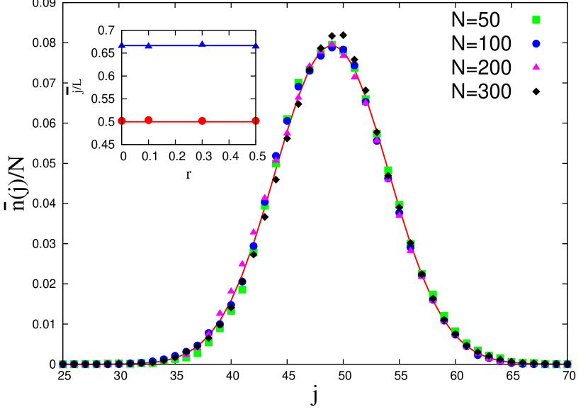
Figure 1: Neutral case: Main figure shows the steady state fraction ${\bar{n}}(j)/N$ in the mutant class $j$ with $\mu=4.9\times 10^{-5}$, $\nu=5.1\times 10^{-5}$ and $L=100$. The distribution is independent of the population size $N$, and matches with the deterministic solution (6) shown by solid line. The inset shows the average fraction of mutations relative to the wildtype as a function of recombination probability $r$ for $L=300$, $N=300$ and $\mu=10^{-4}$ when $\nu=\mu$ ($\bullet$) and $0.5\mu$ ($\blacktriangle$). The solid lines give the theoretical prediction (7).

3.2.2 Recombining population

When the recombination probability is equal to half, as the sequence loci evolve independently, the results from single locus theory are expected to hold. In this case, the frequency of mutations is given exactly by (Wright, 1931; Durrett, 2008)

$${\bar{j}}_{1}=\frac{\mu}{\mu+\nu}$$ (11)

Thus the average number of mutations in the two limiting cases, namely for a nonrecombining population ($r=0$) and a freely recombining one ($r=1/2$), is same. Furthermore, the results of our numerical simulations displayed in the inset of Fig. 1 for $0\leq r\leq 1/2$ show that the average fraction $q$ is independent of the recombination probability.

3.3 FINITE POPULATION UNDER SELECTION

3.3.1 Effect of sequence length

Our numerical simulations show that, unlike in the deterministic case, the fraction of deleterious mutations initially varies with the sequence length and approaches a constant value for long enough sequences. Motivated by the discussion for the deterministic model, we consider the three cases when the sequence length is large.

1. The limit in which $\mu,\nu,s$ are kept fixed but the sequence length is increased has been studied in previous works to gauge the effect of Hill-Robertson interference on the fraction of deleterious mutations (Comeron et al., 1999; Kaiser and Charlesworth, 2009) and to understand the effect of nonrecombining regions of different lengths in the genome of various species (Comeron et al., 1999; Campos et al., 2012). Here for a given $Ns$, the average fraction of deleterious mutations is found to increase with increasing sequence length, but saturates to a finite constant smaller than unity for long sequences. Our simulation data (not shown) is also consistent with this observation.

2. When $U_{d}$ and $\nu$ are kept finite and sequence length is increased, our simulations show that for long enough sequences, the average number of deleterious mutations ${\bar{j}}$ is a constant, as in the deterministic model.

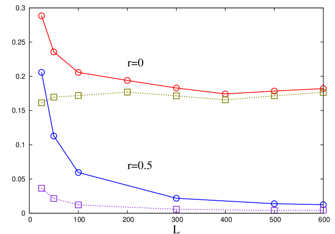
Figure S1: Variation of minimum number $j_{m}$ (broken line with $\square$) and average number $\bar{j}$ (solid line with $\circ$) of deleterious mutations with sequence length $L$ for $N=200$, $s=2\times 10^{-2}$, $U_{d}=10^{-1}$ and $U_{b}=5\times 10^{-2}$.

3. In the rest of the article, we will consider the biologically relevant limit in which the genome mutation rates $U_{b}$ and $U_{d}$ remain finite, as the number of loci in the sequence is increased (Drake et al., 1998). We find that unlike in the deterministic case, here the average fraction of deleterious mutations is finite and sensitive to the beneficial mutation rate. Figure S1 shows that the fraction $q$ decreases to a constant value, as the sequence length is increased. The data shown in the other figures of this article refers to this large-$L$ limit.

3.3.2 Nonrecombining population

The neutral Moran model described in the last section can be straightforwardly generalised to include selection, but we find that the evolution equation for the average number distribution ${\bar{n}}(j)$ does not close in the presence of selection i.e. it involves quantities that can not be expressed in terms of ${\bar{n}}(j)$. Therefore to understand the population size dependence of the average frequency $q$ of deleterious mutations, we use the results obtained in the last two sections, and employ an analytical argument which is described below.

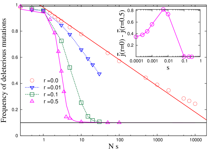
Figure 2: Directional selection and rare beneficial mutations: Figure shows the average frequency of disadvantageous mutations as a function of population size when $U_{d}=10^{-1}$, $U_{b}=10^{-3}$, $s=10^{-2}$ and $L=100$. For nonrecombining population, the line shows the best fit curve $0.087\ln(Ns)+0.98$ to the numerical data and for freely recombining population, (17) is shown. The broken lines joining the numerical data for $r=10^{-2}$ and $r=10^{-1}$ are a guide to the eye. The solid line at the bottom is the deterministic expression (5) and the one at the top shows the prediction (7) from the neutral theory. The inset shows the nonmonotonic behavior of the difference between the deleterious mutations in a nonrecombining and freely recombining population for $N=1000,L=100,U_{d}=10^{-1}$ and $U_{b}=10^{-3}$.

Small and very large populations: Figure 2 and 3 show that the fraction of disadvantageous mutations decreases monotonically with the population size $N$. When the selection is weak ($Ns\ll 1$), the fraction $q$ is expected to be close to the neutral value (7), in agreement with the data in Figs. 2 and  3. For very large populations, the deterministic solution (5) is expected to hold, and Fig. 3 clearly shows that this expectation is borne out by numerical simulations.

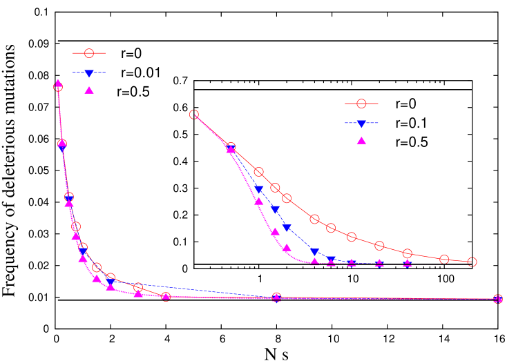
Figure 3: Directional selection and frequent beneficial mutations: Figure shows the average frequency of disadvantageous mutations as a function of population size when $L=100,s=10^{-2},U_{d}=10^{-2},U_{b}=10U_{d}$ (main) and $L=300,s=2\times 10^{-2},U_{d}=10^{-1},U_{b}=0.5U_{d}$ (inset). For freely recombining population, (17) is shown while rest of the curves are a guide to the eye. The solid line at the bottom is the deterministic expression (5) and the one at the top shows the prediction (7) from the neutral theory.

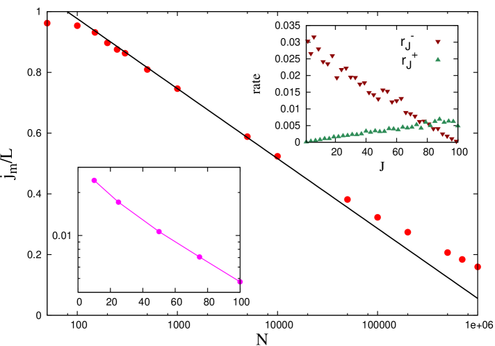
Figure 4: Behavior of least-loaded class: Main figure shows the logarithmic decrease of the deleterious mutation fraction $j_{m}/L$ with population size $N$ when beneficial mutations are rare. The theoretical prediction (15) is shown with a best fit for the intercept as $1.437$. The parameters are $s=10^{-2},U_{d}=10^{-1},U_{b}=10^{-3}$ and $L=100$. Bottom, left inset: Plot to show the exponential decay of $j_{m}/L$ as predicted from (16) when beneficial mutations occur frequently. The line joining the points is a guide to the eye. Here $U_{b}=10^{-1}$ and $U_{d}=10^{-2}$, and the other parameters are same as those in the main figure. Top, right inset: Degeneration and regeneration rates calculated in numerical simulations starting from all the individuals in the best and worst fitness class respectively. Parameters: $L=100,N=50,U_{d}=5\times 10^{-2},U_{b}=5\times 10^{-3}$ and $s=10^{-2}$.

Moderately large populations: We now discuss a rate matching argument that allows us to find the minimum number $j_{m}$ of deleterious mutations in the population. The basic idea is that if beneficial mutations are neglected, due to stochastic fluctuations, all the individuals in the least-loaded fitness class $j_{m}$ will acquire deleterious mutations and it will get lost from the population at a degeneration rate $r_{j_{m}}^{-}$ (Muller, 1964; Haigh, 1978). However due to beneficial back mutations, this process can be reversed and the population in the fitness class $j_{m}$ will be regenerated at a rate $r_{j_{m}}^{+}$. In the stationary state, on equating these two rates, the least-loaded fitness class $j_{m}$ can be found (Goyal et al., 2012). The variation of these rates with the fitness class is shown in the inset of Fig. 4, and we observe that with increasing number of deleterious mutations, the degeneration rate decreases while the regeneration rate increases. This is a direct consequence of the fact that for the fitness-dependent mutation scheme considered here (refer MODELS), the total deleterious mutation rate $(L-j)\mu$ decreases with increasing $j$, but the beneficial mutation rate $j\nu$ decreases with decreasing $j$.

In the absence of beneficial mutations, as shown in Appendix C, the average number of individuals in the least-loaded fitness class $J$ is given by $n_{J}=NX_{J}^{(0)}(J)=N(1-\mu/s)^{L-J}$ which grows exponentially with $J$. As a result, an initially fast-clicking ratchet with $n_{J}s\ll 1$ crosses over to a slow-clicking ratchet with $n_{J}s\gg 1$, when $n_{J}s$ is of order unity (Haigh, 1978; Jain, 2008). Using a diffusion theory for the slow ratchet (Stephan et al., 1993; Gordo and Charlesworth, 2000; Jain, 2008), we find that when $n_{J}\gg 1$, the degeneration rate is given by

$$r_{J}^{-}=\sqrt{\frac{N{X}^{(0)}_{J}(J)c^{3}s^{3}}{\pi}}~{}e^{-csN{X}_{J}^{(0)}(J)}$$ (12)

where

$${X}_{J}^{(0)}(J)\approx e^{-\frac{U_{d}}{s}\left(1-\frac{J}{L}\right)}$$ (13)

and $c$ is a number of order unity (Neher and Shraiman, 2012; Metzger and Eule, 2013). When deleterious mutations are absent, a maladapted population adapts at a rate that depends on the number $NU_{b}$ of beneficial mutants produced per generation. For $NU_{b}\ll 1$, the beneficial mutants arise one at a time and go to fixation sequentially, while they interfere with each other for $NU_{b}\gg 1$ (Gerrish and Lenski, 1998). The regeneration rate in these two parameter regimes is given by (Park et al., 2010; Goyal et al., 2012)

$$r_{J}^{+}\sim 2sNU_{b}~{}(J/L)~{},~{}NU_{b}\ll 1$$

$$r_{J}^{+}\sim \frac{s\ln N}{\ln^{2}U_{b}}~{}\frac{f(J)}{L}~{},~{}NU_{b}\gg 1$$ (14)

where, our numerical simulations for large populations indicate that $f(J)$ is of the form $\delta_{1}\sqrt{J}+\delta_{2}J$. The above equation shows that the rate $r_{J}^{+}$ depends weakly on $N$, and increases linearly with $J$ for large $J$.

i. Rare beneficial mutations ($U_{b}\ll U_{d}$): An expression for $j_{m}$ can be obtained by matching the rates (12) and (14). But as the degeneration rate decays fast with $N$ whereas regeneration rate depends weakly on population size, we may treat the rate $r^{+}_{j_{m}}$ as a constant in $N$. This simplification implies that $r_{j_{m}}^{-}\sim e^{-csN{X}_{j_{m}}^{(0)}(j_{m})}\sim 1$ which immediately leads to

$$\frac{j_{m}}{L}\sim-\frac{s}{U_{d}}\ln(Ns)$$ (15)

Our analytical result (15) is compared with the results of numerical simulations in Fig. 4 and for a wide range of population sizes, we see a good agreement. Figure S2 shows that the average population fraction is distributed over a narrow range of fitness classes (Li, 1987), and therefore we may expect ${\bar{j}}$ to behave in a manner similar to $j_{m}$. Indeed as shown in Fig. 2, the average fraction of disadvantageous mutations also decreases logarithmically with population size, albeit with a prefactor smaller than $s/U_{d}$.

ii. Frequent beneficial mutations ($U_{b}\gg U_{d}$): When $U_{b}\gg U_{d}$, the average frequency of deleterious mutations lies between the neutral value $\mu/\nu$ (refer (7)) and the deterministic value $\mu/(s+\nu)$ (refer (5)), and thus $q\ll 1$ for a wide range of population sizes. This implies that $j_{m}/L$ is also small compared to unity. Using this in (13), and that the degeneration rate $r_{j_{m}}^{+}$ is linear in $j_{m}$, we have

$$\frac{j_{m}}{L}\sim e^{-csNe^{-U_{d}/s}}$$ (16)

which decreases exponentially fast with population size and is consistent with our numerical observations shown in the inset of Fig. 4. Same behaviour is observed for the average fraction of deleterious mutations ${\bar{j}}/L$, refer Fig. 3.

3.3.3 Recombining population

Having discussed the case of complete linkage ($r=0$), we now turn to the limit of completely unlinked loci ($r=1/2$) where single locus theory applies. When selection is present, a diffusion theory calculation (Wright, 1931) gives the frequency of deleterious mutations for a haploid population to be (Kimura et al., 1963)

$${\bar{j}}_{1}=\frac{\mu}{\mu+\nu}~{}\frac{{}_{1}F_{1}(2N\mu+1,2N(\mu+\nu)+1,-2Ns)}{{}_{1}F_{1}(2N\mu,2N(\mu+\nu),-2Ns)}$$ (17)

where ${}_{1}F_{1}(a,b,z)$ is the confluent hypergeometric function. For $s=0$, the above expression reduces to (11). When $Ns$ is small, we have

$${\bar{j}}_{1}=\left(1+\frac{\nu}{\mu}e^{2Ns}\right)^{-1}$$ (18)

which may be obtained either from (17) (Li, 1987; Bulmer, 1991; Kondrashov, 1995; Lande, 1998) or a rate matching argument (Bulmer, 1991; Lande, 1998). When $Ns$ is large, (17) approaches $\mu/s$ (Kimura et al., 1963) as one would also expect from the deterministic solution (5). Thus as Fig. 2 and 3 show, the fraction $q$ decreases exponentially fast in a reverse sigmoidal fashion, as the population size $N$ is increased when there is no linkage between loci.

As in the two extreme cases of complete linkage and no linkage, for $0<r<1/2$, we discern three distinct regimes in the behavior of the fraction $q$ of disadvantageous mutations. Our numerical data in Figs. 2 and 3 shows that the fraction $q$ is roughly constant in population size and recombination rate when the population is small or very large. But for moderately large population, $q$ decreases with increasing population size and the general effect of recombination is to decrease the equilibrium frequency of the deleterious mutations.

4 Discussion

In this article, we examined the stationary state of a model in which both beneficial and deleterious mutations can occur. The multilocus model studied here differs from that in previous works (Gordo and Charlesworth, 2001; Goyal et al., 2012) where these mutation rates are assumed to be independent of the fitness. Here we considered a biologically realistic situation of forward and backward mutations where the rates depend linearly on the logarithmic fitness. In the general scenario where compensatory mutations can occur, nonlinear relationship between the mutation rates and logarithmic fitness has been experimentally observed (Silander et al., 2007). Here we are mainly concerned with the variation of the average number ${\bar{j}}$ of deleterious mutations with the population size.

4.1 Exact bounds on the number of deleterious mutations

For an infinitely large and nonrecombining population, exact results for the population frequency have been obtained for special choice of parameters (Woodcock and Higgs, 1996; Maia et al., 2003; Etheridge et al., 2009; Pfaffelhuber et al., 2012), and here these results were generalised to obtain exact stationary  state and dynamics. Since we consider non-epistatic fitnesses, the stationary state solution does not depend on the recombination rate (Eshel and Feldman, 1970). Moreover as the deterministic limit corresponds to very strong selection which is not favorable for disadvantageous mutations, this analysis provides a lower bound on the average number ${\bar{j}}$ of deleterious mutations.

The upper bound on ${\bar{j}}$ can be found by considering the neutral limit for a finite population. For completely linked loci, we calculated the average frequency of mutations (relative to the wildtype) exactly, and found it to be independent of the population size. Although the latter result is known from previous studies on one locus models (Durrett, 2008), to our knowledge, such a result has not been obtained using a multilocus model. Using numerical simulations and the known results for freely recombining population (Wright, 1931; Durrett, 2008), we found that the number ${\bar{j}}$ is independent of the recombination rate in the neutral limit as well. This happens because in the absence of selection, as random genetic drift creates positive and negative linkage disequilibrium (LD) with equal probability, the average LD vanishes (Hill and Robertson, 1968; Hadany and Comeron, 2008) and therefore the average number ${\bar{j}}$ is not affected by recombination. It should however be noted that the higher moments of the number of mutations may depend on both the recombination rate and population size (Hill and Robertson, 1968).

4.2 Effect of drift, selection and recombination

To get an insight into the problem when both selection and population size are finite and recombination is absent, we used a rate matching argument which states that stationarity is achieved when the rate at which the least-loaded fitness class is lost due to deleterious mutations equals the rate at which it is regenerated by beneficial mutations (Goyal et al., 2012). A similar argument has been used previously by Bulmer (1991), but in a single locus setting, to arrive at the equilibrium fraction of deleterious mutations given in (18). In recent years, some analytical understanding of the rate at which an asexual population declines in fitness (Stephan et al., 1993; Gordo and Charlesworth, 2000; Jain, 2008; Etheridge et al., 2009; Waxman and Loewe, 2010; Neher and Shraiman, 2012; Metzger and Eule, 2013) and adapts (Gerrish and Lenski, 1998; Wilke, 2004; Rouzine et al., 2008; Desai and Fisher, 2007; Park et al., 2010) has become available in multilocus models. Using these results and the rate balancing argument described above, we found analytical expressions for the minimum number of deleterious mutations that a finite asexual population under selection carries in the stationary state.

For a nonrecombining population, our main result is that the average fraction $q$ of deleterious mutations decreases from the neutral value (7) towards the deterministic fraction (5), as population size is increased. If beneficial mutations are rare ($U_{b}\ll U_{d}$), as is the case in adapting microbial populations (Sniegowski and Gerrish, 2010), $q$ changes logarithmically with population size. In an adaptation experiment on bacteriophage, it was observed that when the population size is increased by a factor ten, the logarithmic fitness increased mildly (Silander et al., 2007), which is consistent with the weak $N$-dependence seen here. Experimental data (Zeng, 2010; Schrider et al., 2013) on Drosophila shows that the mutation rate from preferred to unpreferred codon is twice as much as that for the reverse mutations. In such a case where $U_{b}\sim U_{d}$, as the inset of Fig. 3 indicates, $q$ decreases faster than the logarithm of population size, but we do not have an analytical form for it. However in the extreme case when $U_{b}\gg U_{d}$, we find that the fraction $q$ decreases exponentially fast with the population size. Similar qualitative behaviour, namely, the decrease in ${\bar{j}}$ with increasing population size is seen when recombination is nonzero, refer Figs. 2 and 3. When the population size is kept fixed and the selection coefficient is increased, the average fraction of deleterious mutations decreases as one would intuitively expect (data not shown). Although the rate balancing argument used here explains the population size dependence of the fraction of deleterious mutations, we have not been able to obtain a complete analytical understanding of its variation with selection coefficient since the $s$-dependence of the function $c$ in the degeneration rate in (12) is not known. We also performed numerical simulations keeping the product $Ns$ constant ($=10$), and find that ${\bar{j}}$ is not a function of $Ns$ unlike the one locus theory prediction (17). For $s=0.005$, we obtained ${\bar{j}}=13.7$ which increased to $28.8$ on halving $s$ which suggests that it depends more strongly on $s$ than $N$ which is consistent with (15).

For a given $Ns$, we find that the recombination reduces the frequency of the deleterious mutations (also see (Barton, 2010)). As discussed above, in a finite population, due to random genetic drift, both positive and negative LD are created. If LD is positive, the population consists of individuals with extreme fitnesses on which selection can act efficiently and thus removes the LD. On the other hand, when LD is negative, as most of the individuals are likely to have similar fitnesses, selection is ineffective in removing LD. Thus in the presence of selection, the average LD in a nonrecombining population is negative (Felsenstein, 1974; Hadany and Comeron, 2008). But once recombination is introduced, it will create individuals with extreme fitnesses thereby helping selection to weed out the deleterious mutations, and thus decreasing ${\bar{j}}$. The effect is large for intermediate values of $Ns$ since this regime corresponds to both selection and drift having a strong effect. From the results in the neutral and deterministic limit, we expect that the difference in the number of deleterious mutations carried by a nonrecombining and recombining population is nearly zero when $s\ll 1/N$ (weak selection) and $s\gg 1/N$ (strong selection). Thus, as shown in the inset of Fig. 2, the maximum advantage of recombination occurs at an intermediate value of selection coefficient as has also been observed in other studies (Gordo and Campos, 2008).

Although recombination reduces the number of deleterious mutations, the extent to which it does so depends on how common the beneficial mutations are compared to the deleterious ones. In an adapting asexual population where beneficial mutations occur rarely (Sniegowski and Gerrish, 2010), even slight recombination reduces ${\bar{j}}$ considerably indicating the advantage of recombination during adaptation (Barton and Charlesworth, 1998; Hadany and Comeron, 2008). On the other hand, in the codon bias problem where back mutation rates are comparable to the forward ones (Zeng, 2010; Schrider et al., 2013), the fraction of unpreferred codons is given by (18) if the loci are assumed to be completely unlinked, but as the inset of Fig. 3 shows, linkage increases the unpreferred codon frequency moderately (Comeron et al., 1999; McVean and Charlesworth, 2000; Charlesworth et al., 2009).

4.3 Effect of background selection - an application

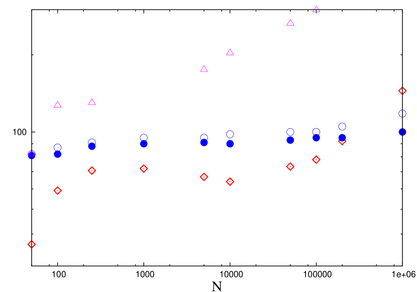
Figure S3: Figure shows the effective population size $N_{e}$ ($\lozenge$) given by (19) where $j_{m}$ is shown in Fig. 4, and click time of the Muller’s ratchet with deleterious mutation rate $U_{d}^{\prime}$ and selection coefficient $s^{\prime}$, when there are finite number of background selection sites with reversible mutations. The click time of the ratchet for (i) a population of size $N$ and without background selection sites ($\vartriangle$), (ii) a population of size $N$ with background selection sites ($\circ$) and (iii) a population of size $N_{e}$ without background selection sites ($\bullet$) are shown. Parameters: $L=100,s=0.01,U_{d}=0.1,U_{b}=0.001,U_{d}^{\prime}=0.015,s^{\prime}=0.001$.

Background selection is a type of Hill-Robertson effect (Charlesworth, 2012) and is known to increase the rate at which the Muller’s ratchet clicks (Gordo and Charlesworth, 2001; Kaiser and Charlesworth, 2010). In a finite, nonrecombining population with an infinitely long sequence in which both deleterious and beneficial mutations occur at $L$ background selection sites, and deleterious mutations accumulate at rest of the sites (Kaiser and Charlesworth, 2010), we find that the ratchet clicking time is considerably reduced from the situation when there are no background selection sites (see Fig. S3). linIf the background selection sites (BGS) remain at equilibrium in the presence of other linked loci also, they affect the evolutionary dynamics at other sites, and their effect can be quantified by a reduction in the effective population size to the number of individuals carrying the minimum number of deleterious mutations at BGS (Charlesworth, 2012; Gordo and Charlesworth, 2001). Since the minimum number of deleterious mutations in the BGS is $j_{m}$, we require the population fraction in the class $j_{m}$. For large populations with $Ns\gg 1$ where the deterministic theory is expected to hold, using (9) and (13), we obtain

$$N_{e}=Ne^{-\frac{U_{d}(1-\frac{j_{m}}{L})}{s}}$$ (19)

where $j_{m}$ is a function of population size $N$. The ratchet time with background selection for a population of size $N$ is found to be well approximated by the ratchet time without it for a population of size $N_{e}$ as shown in Fig. S3. From the results for $j_{m}$ when $U_{b}\ll U_{d}$, we expect $N_{e}$ in (19) to increase linearly with $N$ for small and large populations. But for the intermediate range of population sizes, using (15) in (19) above, we find the effective population size to be independent of $N$. These predictions were tested numerically and as shown in Fig. S3, the effective population size and the ratchet time remain roughly constant when the actual population size is varied over three orders of magnitude .

5 Conclusions

We close this article by listing some open questions. Here we investigated the effect of linkage using numerical simulations, but an analytical expression for the average ${\bar{j}}$ as a function of recombination probability is desirable. We also considered the specific case of forward and backward mutations, and an extension of these results to the more general case of compensatory mutations would be interesting.

Acknowledgement

The authors thank B. Charlesworth, M. M. Desai, S. Goyal, J. Krug and L. M. Wahl for discussions, and are grateful to B. Charlesworth for useful comments on an earlier version of the manuscript.

Appendix A: Deterministic dynamics and stationary state

Equation (1) is nonlinear in the population fraction due to the first term on the RHS. This nonlinearity can be eliminated by a change of variables from $X(j,t)$ to an unnormalised population variable $Z(j,t)$ which is defined as (Jain and Krug, 2007; Jain and Seetharaman, 2011)

$$Z(j,t)=X(j,t)~{}e^{\int_{0}^{t}dt^{\prime}~{}{\overline{w}}(t^{\prime})}$$ (20)

Then the unnormalised population fraction obeys the following linear differential equation:

$$\frac{\partial{Z}(j)}{\partial t} = -sj~{}{Z}(j,t)-[(L-j)\mu+j\nu]{Z}(j,t)$$ (21)

$$+ (L-j+1)\mu{Z}(j-1,t)+(j+1)\nu{Z}(j+1,t)$$

with boundary conditions

$${Z}(-1,t)={Z}(L+1,t)=0$$ (22)

at all times. The RHS of (21) is a three-term recursion relation (in $j$) with variable coefficients, which is usually not easy to solve.

Inspired by the results of Woodcock and Higgs (1996), we assume that the population fraction ${Z}(j,t)$ is of the following form

$${Z}(j,t)={L\choose j}~{}x_{1}^{j}(t)~{}x_{2}^{L-j}(t)$$ (23)

where $x_{1},x_{2}$ are calculated below. The normalised fraction $X(j,t)$ is then given by (Jain and Krug, 2007; Jain and Seetharaman, 2011)

$$X(j,t) = \frac{Z(j,t)}{\sum_{j^{\prime}=0}^{L}Z(j^{\prime},t)}$$ (24)

$$= {L\choose j}x^{j}(t)~{}(1-x(t))^{L-j}$$ (25)

where $x=x_{1}/(x_{1}+x_{2})$ lies between zero and one. It should be noted that the above form for the population fraction of a fitness class implies that each locus in the sequence contributes independently to the population fraction of a sequence.

Using the ansatz (23) in the boundary conditions (22), we find that $x_{1},x_{2}$ obey linear, coupled differential equations which can be expressed as

$$\frac{\partial}{\partial t}\begin{pmatrix}{x}_{1}\\ {x}_{2}\end{pmatrix}=\begin{pmatrix}-\nu-s&\mu\\ \nu&-\mu\end{pmatrix}~{}\begin{pmatrix}x_{1}\\ x_{2}\end{pmatrix}$$ (26)

On using the ansatz (23) in the bulk equation (21) for which $0<j<L$, we get

$$\frac{j}{x_{1}}\left[\frac{{\partial x}_{1}}{\partial t}+\left(\nu+s\right)x_{1}-\mu x_{2}\right]+\frac{L-j}{x_{2}}\left[\frac{{\partial x}_{2}}{\partial t}-\nu x_{1}+\mu x_{2}\right]=0$$ (27)

However due to (26), the coefficient of $j$ and $L-j$ equals zero for any $0<j<L$. Thus the ansatz (23) is consistent with the bulk equations, and the problem reduces to solving the matrix equation (26). By going to the diagonal basis, we obtain

$$\begin{pmatrix}{x}_{1}(t)\\ {x}_{2}(t)\end{pmatrix}=\begin{pmatrix}\frac{2\mu}{\nu-\mu+s+\sqrt{(\mu-s-\nu)^{2}+4\mu\nu}}&\frac{2\mu}{\nu-\mu+s-\sqrt{(\mu-s-\nu)^{2}+4\mu\nu}}\\ 1&1\end{pmatrix}~{}\begin{pmatrix}e^{\lambda_{+}t}~{}{\tilde{x}}_{1}(0)\\ e^{\lambda_{-}t}~{}{\tilde{x}}_{2}(0)\end{pmatrix}$$ (28)

where the column vectors in the matrix above are the eigenvectors of the matrix on the RHS of (26) corresponding to the eigenvalues $\lambda_{\pm}$, which are given by

$$\lambda_{\pm}=\frac{-\nu-\mu-s\pm\sqrt{(\mu-s-\nu)^{2}+4\mu\nu}}{2}$$ (29)

and ${\tilde{x}}_{1}(0),{\tilde{x}}_{2}(0)$ can be found using the initial condition $X(j,0)$.

In the steady state, the population fraction is obtained by taking the limit $t\to\infty$ in the expressions of $x_{1}(t),x_{2}(t)$ obtained above. Using the fact that the eigenvalue $\lambda_{-}$ in (29) is negative, we find that the steady state fraction $x$ is given by (5).

Appendix B: Moran model for neutral, nonrecombining population

For the Moran process defined in the main text, the probability distribution $P(n(i),t)$ of the number of individuals in the fitness class $i$ evolves according to the following equation:

$$\frac{\partial P(n(i),t)}{\partial t}$$

$$=\sum_{j\neq i}\left[\sum_{n(j)=1}^{N-n(i)}P(n(i)+1,n(j)-1,t)~{}R(n(i)+1\to n(i),n(j)-1\to n(j))\right.$$

$$-\sum_{n(j)=0}^{N-n(i)}P(n(i),n(j),t)~{}R(n(i)\to n(i)-1,n(j)\to n(j)+1)$$

$$+\sum_{n(j)=1}^{N-n(i)}P(n(i)-1,n(j)+1,t)~{}R(n(i)-1\to n(i),n(j)+1\to n(j))$$

$$-\left.\sum_{n(j)=0}^{N-n(i)}P(n(i),n(j),t)~{}R(n(i)\to n(i)+1,n(j)\to n(j)-1)\right]$$ (30)

where $R$ is the rate at which a birth-and-death event occurs, and $P(n(i),n(j),t)$ is the joint distribution of the number of individuals in the $i$th and $j$th fitness class. Using the above equation, it can be seen that the average number of individuals in the fitness class $i$ given by ${{\bar{n}}(i,t)}=\sum_{n(i)=1}^{N}n(i)P(n(i),t)$ changes as

$$\frac{\partial{{\bar{n}}(i,t)}}{\partial t}=\sum_{j\neq i}\sum_{n(i),n(j)}[{R}(n(i)\to n(i)+1,n(j)\to n(j)-1)P(n(i),n(j),t)$$

$$-{R}(n(i)\to n(i)-1,n(j)\to n(j)+1)P(n(i),n(j),t)]$$ (31)

We next find the rates at which the birth-and-death process occurs. For class $i,j=0,...,L$ and $i\neq j$, we have

$$R(n(i)\to n(i)+1,n(j)\to n(j)-1)$$ (32)

$$= (1-\mu_{i}-\nu_{i})\frac{n(i)}{N}\frac{n(j)}{N}+\mu_{i-1}\frac{n(i-1)}{N}\frac{n(j)}{N}+\nu_{i+1}\frac{n(i+1)}{N}\frac{n(j)}{N}$$

with $n(-1)=n(L+1)=0$. In the above equation, the first term on the RHS gives the probability of the event that a birth occurs in the $i$th class, the offspring does not mutate and a death occurs in the $j$th class, while the second and third term give the probability that a birth occurs in a class neighboring the $i$th class, the offspring acquires a mutation and a death occurs in the $j$th class. On using the above equation in (31), after some simple algebra, we get

$$\frac{\partial{{\bar{n}}(i,t)}}{\partial t}=\mu_{i-1}{{\bar{n}}(i-1,t)}+\nu_{i+1}{{\bar{n}}}(i+1,t)-(\mu_{i}+\nu_{i}){{\bar{n}}(i,t)}~{},~{}0\leq i\leq L$$ (33)

which can be easily solved in the stationary state to give (10).

Appendix C: Deterministic solution in the absence of beneficial mutations

Consider an infinitely large, nonrecombining population when only deleterious mutations are allowed. Let $J$ be the least-loaded fitness class so that the frequency $X_{J}^{(0)}(k,t)=0~{},~{}k<J$ at all times. Then the evolution equation (1) reduces to

$$\frac{\partial X_{J}^{(0)}(j,t)}{\partial t} = -(sj+{\bar{w}}_{J}(t))X_{J}^{(0)}(j,t)-(L-j)\mu X_{J}^{(0)}(j,t)$$ (34)

$$+ (L-j+1)\mu X_{J}^{(0)}(j-1,t)~{},~{}J\leq j\leq L$$

where the average fitness ${\bar{w}}_{J}(t)=-s\sum_{k=J}^{L}kX_{J}^{(0)}(k,t)$. In the stationary state, the equation for $j=J$ gives

$${\bar{w}}_{J}=-(L-J)\mu-sJ$$ (35)

On iterating the two-term recursion relation for $X_{J}^{(0)}(j)$, we obtain

$$X_{J}^{(0)}(j)={L-J\choose j-J}\left(\frac{\mu}{s}\right)^{j-J}\left(1-\frac{\mu}{s}\right)^{L-j}~{},~{}\mu<s$$ (36)

For $J=0$, (8) is recovered.

Figure S2: Distribution of the average fraction of individuals in each mutant class for a completely linked sequence for various population sizes, and $L=100$, $U_{d}=10^{-1}$, $U_{b}=10^{-3}$ and $s=10^{-2}$.

References

- Barton and Charlesworth (1998) Barton, N. and B. Charlesworth, 1998 Why sex and recombination? Science 281: 1986–1990.
- Barton (2010) Barton, N., 2010 Genetic linkage and natural selection. Phil. Trans. R. Soc. B 365: 2559–2569
- Bulmer (1991) Bulmer, M., 1991 The selection-mutation-drift theory of synonymous codon usage. Genetics 149: 897–907.
- Campos et al. (2012) Campos, J. L., B. Charlesworth, and P. R. Haddrill, 2012 Molecular evolution in non recombining regions of the Drosophila melanogaster genome. Genome Bio Evol. 4(3): 278–288.
- Charlesworth (2012) Charlesworth, B., 2012 The effects of deleterious mutations on evolution at linked sites. Genetics 190: 5–22.
- Charlesworth et al. (2009) Charlesworth, B., A. J. Betancourt, and V. B. Kaiser, 2009 Genetic recombination and molecular evolution. Cold Spring Harb Symp Quant Biol. 74: 177–186.
- Comeron et al. (1999) Comeron, J. M., M. Kreitman, and M. Aguadé, 1999 Natural selection on synonymous sites is correlated with gene length and recombination in Drosophila. Genetics 151: 239–249.
- Desai and Fisher (2007) Desai, M. and D. Fisher, 2007 Beneficial mutation-selection balance and the effect of linkage on positive selection. Genetics 176: 1759–1798.
- Drake et al. (1998) Drake, J. W., B. Charlesworth, D. Charlesworth, and J. F. Crow, 1998 Rates of spontaneous mutation. Genetics 148: 1667–1686.
- Durrett (2008) Durrett, R., 2008 Probability Models for DNA Sequence Evolution. Springer, New York.
- Eshel and Feldman (1970) Eshel, I. and M. Feldman, 1970 On the evolutionary effect of recombination. Theo. Pop. Biol. 1: 88–100.
- Estes and Lynch (2003) Estes, S. and M. Lynch, 2003 Rapid fitness recovery in mutationally degraded lines of Caenorhabditis elegans. Evolution 57: 1022–1030.
- Etheridge et al. (2009) Etheridge, A., P. Pfaffelhuber, and A. Wakolbinger, 2009 How often does the ratchet click? facts, heuristics, asymptotics. In J. Blath, P. Mörters, and M. Scheutzow (Eds.), Trends in Stochastic Analysis, London Mathematical Society Lecture Note Series 353, pp. 365–390. Cambridge University Press.
- Ewens (2004) Ewens, W., 2004 Mathematical Population Genetics. Springer, Berlin.
- Feller (2000) Feller, W., 2000 An introduction to probability theory and its applications, Vol. I. John Wiley and sons.
- Felsenstein (1974) Felsenstein, J., 1974 The evolutionary advantage of recombination. Genetics 78: 737–756.
- Gerrish and Lenski (1998) Gerrish, P. J. and R. E. Lenski, 1998 The fate of competing beneficial mutations in an asexual populations. Genetica 102: 127–144.
- Gordo and Campos (2008) Gordo, I. and P.R.A. Campos, 2008 Sex and deleterious mutations. Genetics 179: 621–626.
- Gordo and Charlesworth (2000) Gordo, I. and B. Charlesworth, 2000 The degeneration of asexual haploid populations and the speed of Muller’s ratchet. Genetics 154: 1379–1387.
- Gordo and Charlesworth (2001) Gordo, I. and B. Charlesworth, 2001 The speed of Muller’s ratchet with background selection, and the degeneration of Y chromosomes. Genet. Res. 78: 149–161.
- Goyal et al. (2012) Goyal, S., D. J. Balick, E. R. Jerison, R. A. Neher, B. I. Shraiman, and M. M. Desai, 2012 Dynamic mutation selection balance as an evolutionary attractor. Genetics 191: 1309–1319.
- Hadany and Comeron (2008) Hadany, L. and J. M. Comeron, 2008 Why are sex and recombination so common? Ann. N. W. Acad. Sci 1133: 26–43.
- Haigh (1978) Haigh, J., 1978 The accumulation of deleterious genes in a population - Muller’s ratchet. Theoret. Population Biol. 14: 251–267.
- Hershberg and Petrov (2008) Hershberg, R. and D. A. Petrov, 2008 Selection on codon bias. Annu. Rev. Genet. 42: 287–299.
- Hill and Robertson (1966) Hill, W. G. and A. Robertson, 1966 The effect of linkage on limits to artificial selection. Genet. Res., Camb. 8: 269–294.
- Hill and Robertson (1968) Hill, W. G. and A. Robertson, 1968 Linkage disequilibrium in finite populations. Theoretical and Applied Genetics 38: 226–231.
- Howe and Denver (2008) Howe, D. K. and D. R. Denver, 2008 Muller’s ratchet and compensatory mutation in Caenorhabditis briggsae mitochondrial genome evolution. BMC Evolutionary Biology 8: 62.
- Jain (2008) Jain, K., 2008 Loss of least-loaded class in asexual populations due to drift and epistasis. Genetics 179: 2125–2134.
- Jain and Krug (2007) Jain, K. and J. Krug, 2007 Adaptation in simple and complex fitness landscapes. In U. Bastolla, M. Porto, H. Roman, and M. Vendruscolo (Eds.), Structural Approaches to Sequence Evolution: Molecules, Networks and Populations, pp. 299–340. Springer, Berlin.
- Jain and Seetharaman (2011) Jain, K. and S. Seetharaman, 2011 Nonlinear deterministic equations in biological evolution. J. Nonlin. Math. Phys. 18: 321–338.
- Kaiser and Charlesworth (2009) Kaiser, V. B. and B. Charlesworth, 2009 The effects of deleterious mutations on evolution in non-recombining genomes. Trends in Genetics 25: 339–348.
- Kaiser and Charlesworth (2010) Kaiser, V. B. and B. Charlesworth, 2010 Muller’s ratchet and the degeneration of the Drosophila miranda neo-Y chromosome. Genetics 185: 339–348.
- Kimura et al. (1963) Kimura, M., T. Maruyama, and J. F. Crow, 1963 The mutation load in small populations. Genetics 48: 1303–1312.
- Kondrashov (1995) Kondrashov, A., 1995 Contamination of the genome by very slightly deleterious mutations: why have we not died 100 times over? J. theor. Biol. 175: 583–594.
- Lande (1998) Lande, R., 1998 Risk of population extinction from fixation of deleterious and reverse mutations. Genetica 102-103: 21–27.
- Li (1987) Li, W. H., 1987 Models of nearly neutral mutations with particular implications for nonrandom usage of synonymous codons. J Mol Evol 24: 337–345.
- Maia et al. (2003) Maia, L. P., D. F. Botelho, and J. F. Fontanari, 2003 Analytical solution of the evolution dynamics on a multiplicative-fitness landscape. J. Math. Biol. 47: 453–456.
- McVean and Charlesworth (1999) McVean, G. A. T. and B. Charlesworth, 1999 A population genetic model for the evolution of synonymous codon usage: patterns and predictions. Genet. Res., Camb. 74: 145–158.
- McVean and Charlesworth (2000) McVean, G. A. T. and B. Charlesworth, 2000 The effects of Hill-Robertson interference between weakly selected mutations on patterns of molecular evolution and variation. Genetics 155: 929–944.
- Metzger and Eule (2013) Metzger, J. J. and S. Eule, 2013 Distribution of the fittest individuals and the rate of Muller’s ratchet in a model with overlapping generations. PLoS Comp. Biol 9: e1003303.
- Muller (1964) Muller, H. J., 1964 The relation of recombination to mutational advance. Mutation Res. 1: 2–9.
- Neher and Shraiman (2012) Neher, R. and B. Shraiman, 2012 Fluctuations of fitness distributions and the rate of Muller’s ratchet. Genetics 191: 1283 – 1293.
- Nowak et al. (2014) Nowak, S., J. Neidhart, I.G. Szendro, and J. Krug, 2014 Multidimensional epistasis and the transitory advantage of sex. arXiv: 1403.6406v1.
- Park et al. (2010) Park, S.-C., D. Simon, and J. Krug, 2010 The speed of evolution in large asexual populations. J. Stat. Phys. 138: 381–410.
- Pfaffelhuber et al. (2012) Pfaffelhuber, P., P. Staab, and A. Wakolbinger, 2012 Muller’s ratchet with compensatory mutations. Ann. Appl. Probab. 22: 2108 – 2132.
- Plotkin and Kudla (2011) Plotkin, J. B. and G. Kudla, 2011 Synonymous but not the same: the causes and consequences of codon bias. Nat. Rev. Genet. 12: 32–42.
- Rouzine et al. (2008) Rouzine, I., E. Brunet, and C. Wilke, 2008 The traveling-wave approach to asexual evolution: Muller’s ratchet and speed of adaptation. Theo. Pop. Biol. 73: 24–46.
- Schrider et al. (2013) Schrider, D. R., D. Houle, M. Lynch, and M. W. Hahn, 2013 Rates and genomic consequences of spontaneous mutational events in Drosophila melanogaster. Genetics 194: 937–954.
- Seetharaman and Jain (2014) Seetharaman, S. and K. Jain, 2014 Adaptive walks and distribution of beneficial fitness effects. Evolution 68: 965–975.
- Silander et al. (2007) Silander, O., O. Tenaillon, and L. Chao, 2007 Understanding the evolutionary fate of finite populations: the dynamics of mutational effects. PLoS Biology 5: 922–931.
- Sniegowski and Gerrish (2010) Sniegowski, P. D. and P. J. Gerrish, 2010 Beneficial mutations and the dynamics of adaptation in asexual populations. Phil. Trans. R. Soc. B 365: 1255–1263.
- Stephan et al. (1993) Stephan, W., L. Chao, and J. G. Smale, 1993 The advance of Muller’s ratchet in a haploid asexual population - approximate solutions based on diffusion theory. Genet. Res. Camb. 61: 225–232.
- Waxman and Loewe (2010) Waxman, D. and L. Loewe, 2010 A stochastic model for a single click of Muller’s ratchet. J. theor Biol. 264: 1120–1132.
- Whitlock (2000) Whitlock, M. C., 2000 Fixation of new alleles and the extinction of small populations: drift load, beneficial alleles, and sexual selection. Evolution 54: 1855–1861.
- Wiehe (1997) Wiehe, T., 1997 Model dependency of error thresholds: the role of fitness functions and contrasts between the finite and infinite sites models. Genet. Res. Camb. 69: 127–136.
- Wilke (2004) Wilke, C. O., 2004 The speed of adaptation in large asexual populations. Genetics 167: 2045–2053.
- Woodcock and Higgs (1996) Woodcock, G. and P. G. Higgs, 1996 Population evolution on a multiplicative single-peak fitness landscape. J. theor. Biol. 179: 61–73.
- Wright (1931) Wright, S., 1931 Evolution in Mendelian populations. Genetics 16: 97–159.
- Zeng (2010) Zeng, K., 2010 A simple multiallele model and its application to identifying preferred-unpreferred codons using polymorphism data. Mol. Biol. Evol. 27 (6): 1327–1337.
SUPPORTING INFORMATION