Collective pairing of resonantly coupled microcavity polaritons

Abstract

We consider the possible phases of microcavity polaritons tuned near a bipolariton Feshbach resonance. We show that, as well as the regular polariton superfluid phase, a “molecular” superfluid exists, with (quasi-)long-range order only for pairs of polaritons. We describe the experimental signatures of this state. Using variational approaches we find the phase diagram (critical temperature, density and exciton-photon detuning). Unlike ultracold atoms, the molecular superfluid is not inherently unstable, and our phase diagram suggests it is attainable in current experiments.

The wealth of physics explored with ultracold atomic gases Bloch et al. (2008) relies on the ability to tune parameters such as the interaction strength. A crucial tool to achieve this is the Feshbach resonance mechanism Chin et al. (2010): By using a magnetic field one may vary the detuning $\nu$ between two channels (hyperfine states) of the atoms; a closed channel (bound molecule) and open (scattering) channel. When $\nu$ is large and positive, the closed channel is far above open channel atoms, the formation of molecules is energetically suppressed and atoms scatter with a weakly attractive effective interaction. When $\nu$ is large and negative, atoms are paired into molecules and the effective interaction is weakly repulsive. Near resonance ($\nu\simeq 0$), the interaction is very large. This enables tunable pairing and regimes of strong correlations, allowing many interesting possibilities both at few- and many-body level.

Ultracold atom experiments are however intrinsically metastable, not true minima of the free energy. Three-body collisions must be avoided to prevent relaxation to, e.g., a solid phase. Also, Feshbach molecular states are highly rovibrationally excited states and can relax to lower states. Exploring regimes of strong interactions while suppressing such relaxation processes is inherently challenging. For fermionic atoms, Pauli exclusion suppresses scattering rates, so strongly interacting regimes can be accessed. In this case there is a smooth crossover between a Bardeen-Cooper-Schrieffer (BCS) condensate of weakly attractive fermions and a Bose-Einstein condensate (BEC) of repulsive molecules Ketterle and Zwierlein (2008); Leggett and Zhang (2012).

The situation for bosons near a Feshbach resonance differs substantially: Unlike fermions, both a condensate of molecules and a condensate of unpaired bosons can exist. As discussed below this means that a “molecular” superfluid phase with no off-diagonal long-range order (ODLRO) for atoms can arise, with a further symmetry breaking phase transition between “atomic” and “molecular” superfluids. Bosonic mixtures have attracted considerable theoretical interest Timmermans et al. (1999); Mueller and Baym (2000); Jeon et al. (2002); Kuklov et al. (2004a, b); Radzihovsky et al. (2004); Romans et al. (2004); Radzihovsky et al. (2008); Basu and Mueller (2008); Zhou et al. (2008); Koetsier et al. (2009); Bhaseen et al. (2009); Radzihovsky and Choi (2009); Hohenadler et al. (2010); Ejima et al. (2011); Bhaseen et al. (2012); Zhou and Mashayekhi (2013). However, experiments have been limited by stability issues: The molecular superfluid phase generally requires high densities Basu and Mueller (2008); Koetsier et al. (2009), where three body losses are significant Rem et al. (2013). There have been suggestions to use optical lattices Kuklov et al. (2004a) to reach the strongly interacting regime while avoiding high densities, but to date, molecular pairing phases of bosonic atoms remain elusive.

Microcavity polaritons Kavokin et al. (2007); Carusotto and Ciuti (2013), the quasiparticles resulting from strong coupling between cavity photons and quantum well excitons, do not suffer the metastability problems of cold atoms and so present a more promising venue to study bosonic pairing phases. Microcavity polaritons have been observed to form a BEC Kasprzak et al. (2006); Balili et al. (2007), and, as recently discussed Wouters (2007); Carusotto et al. (2010), interactions between polaritons with opposite polarizations can support either a bound state (bipolariton) or a scattering resonance depending on the exciton-photon detuning. Several signatures of this physics have been seen Saba et al. (2000); Borri et al. (2003); Wen et al. (2013a), including recent direct observations of the scattering resonance vs detuning Takemura et al. (2014, 2013). Polaritons are expected not to suffer from the issues of three body inelastic losses Basu and Mueller (2008); Koetsier et al. (2009); Rem et al. (2013) which plague cold bosonic atoms: Unlike ultracold atoms, a polariton BEC is not a metastable state, rather it is the minimum free energy state as long as the polariton population is conserved. In addition, there is no deeply bound molecular state below the bipolariton. Polaritons do have a finite lifetime, however recent experiments have demonstrated a 5–10 fold increase in lifetime Wen et al. (2013b), leading to a system very close to thermal equilibrium. A full non-equilibrium treatment of spin dynamics and relaxation is beyond the scope of this work. However, unlike cold atoms, such losses are not intrinsically linked to the resonance physics, and so they can be addressed and improved independently. Thus, polaritons may form a more promising venue to study pairing phases.

In this Letter we explore the phase diagram of collective paired phases arising from a bipolariton resonance in microcavities. By using the cavity-exciton detuning to tune the interactions Wouters (2007); Carusotto et al. (2010), we reveal a phase transition between atomic (i.e. polariton) and molecular (i.e. bipolariton) BEC phases. We show that temperatures and detunings required for typical materials such as GaAs are attainable and we discuss experimental signatures for detecting such phases.

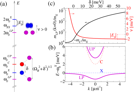
Figure 1: (Color online) (a) Cartoon of one- and two-particle energy scales, showing how the cavity(C)–exciton(X) detuning $\delta$ determines the inter-channel detuning $\nu$. (b) Lower (LP) and upper (UP) polariton dispersions (solid [magenta] lines), along with the C (X) dispersion (dashed [red (blue)] lines) for $\delta=2$ meV. (c) Dependence of the rescaled polariton mass at zero momentum $m_{LP}({\mathbf{k}}=0)/m_{X}$ (left [black]) and of the inter-channel detuning $\nu$ (right [red]) on $\delta$. Plots are for GaAs parameters ($\Omega_{R}=4.4$ meV, $|E_{b}|=2$ meV Wouters (2007), photon mass $m_{C}=10^{-4}m_{X}$, exciton mass $m_{X}=0.4m_{e}$).

Model —

In the model we consider, bipolaritons play the rôle of closed channel molecules, while the two (polarized) LP modes are the open channel modes. The inter-channel detuning is (see Fig. 1), with $E_{b}$ the biexciton binding energy and $2\omega_{{\mathbf{k}}}^{LP}=\omega_{{\mathbf{k}}}^{C}+\omega_{{\mathbf{k}}}^{X}-\sqrt{(\omega_{{\mathbf{k}}}^{C}-\omega_{{\mathbf{k}}}^{X})^{2}+\Omega_{R}^{2}}$, where both the exciton and cavity photon dispersions are quadratic, $\omega^{C,X}_{{\mathbf{k}}}=\omega^{C,X}_{{\mathbf{0}}}+\frac{k^{2}}{2m_{C,X}}$. In fact, as discussed later and in SM , the bipolariton bound state is almost identical to a biexciton. However, it possesses a non-zero photon component and for this reason we refer to it as a bipolariton. Even a small photon content has important consequences in breaking the degeneracy between dark and bright excitonic states SM . The inter-channel detuning $\nu$ can be controlled by varying the cavity-exciton detuning $\delta=\omega_{0}^{C}-\omega_{0}^{X}$ (see Fig. 1). A resonant enhancement of the interactions occurs near the bare resonance $\nu\simeq 0$.

We derive the many-body properties of resonantly coupled polaritons by considering a two-channel model, which includes both LPs in the right- and left-circular polarization basis, $\hat{\psi}_{\uparrow,\downarrow}$ and bipolariton $\hat{\psi}_{m}$ fields. One could, alternatively, work with a single-channel model with no explicit bipolariton field, at the expense of needing a finite range attractive potential $U^{\uparrow\downarrow}({\mathbf{r}})$ supporting a resonant bound state Gurarie and Radzihovsky (2007). Such an approach unnecessarily complicates the derivation of many-body physics, while a single-channel model with a contact potential cannot describe deeply bound bipolariton states.

The effective two-channel polariton model has been derived starting from a model describing coupled exciton, biexction and photon fields and rotating to the LP $\hat{\psi}_{\uparrow,\downarrow}$ and bipolariton $\hat{\psi}_{m}$ fields (see the scheme in Fig. 1 (a)). This yields the following grand-canonical Hamiltonian written in momentum space, $\hat{\psi}_{\sigma}({\mathbf{r}})=\sum_{{\mathbf{k}}}e^{i{\mathbf{k}}\cdot{\mathbf{r}}}\hat{a}_{{\mathbf{k}}\sigma}/\sqrt{\mathcal{A}}$ (where ${\mathbf{k}}$ is the in-plane [2D] momentum, $\mathcal{A}$ the system area, and $\hbar=1$ throughout):

$$\hat{H}=\sum_{\sigma=\uparrow,\downarrow,m}\sum_{{\mathbf{k}}}\hat{a}_{{\mathbf{k}}\sigma}^{\dagger}\left(\epsilon_{{\mathbf{k}}\sigma}-\mu_{\sigma}\right)\hat{a}_{{\mathbf{k}}\sigma}\\ +\displaystyle\frac{1}{\mathcal{A}}\sum_{\sigma\sigma^{\prime}}\sum_{{\mathbf{k}},{\mathbf{k}}^{\prime},{\mathbf{q}}}\displaystyle\frac{U_{{\mathbf{k}}{\mathbf{k}}^{\prime}{\mathbf{q}}}^{\sigma\sigma^{\prime}}}{2}\hat{a}_{{\mathbf{k}}\sigma}^{\dagger}\hat{a}_{{\mathbf{k}}^{\prime}\sigma^{\prime}}^{\dagger}\hat{a}_{{\mathbf{k}}^{\prime}-\frac{{\mathbf{q}}}{2}\sigma^{\prime}}\hat{a}_{{\mathbf{k}}+\frac{{\mathbf{q}}}{2}\sigma}\\ +\displaystyle\frac{1}{\sqrt{\mathcal{A}}}\sum_{{\mathbf{k}},{\mathbf{Q}}}\displaystyle\frac{g_{{\mathbf{k}}{\mathbf{Q}}}}{2}\left(\hat{a}_{{\mathbf{k}}+\frac{{\mathbf{Q}}}{2}\uparrow}^{\dagger}\hat{a}_{-{\mathbf{k}}+\frac{{\mathbf{Q}}}{2}\downarrow}^{\dagger}\hat{a}_{{\mathbf{Q}}m}+\text{h.c.}\right)\;.$$ (1)

Here $\epsilon_{{\mathbf{k}}\uparrow,\downarrow}=\omega_{{\mathbf{k}}}^{LP}-\omega_{0}^{LP}$ is the full LP dispersion (see Fig. 1 (b)). The coupling $g_{{\mathbf{k}}{\mathbf{Q}}}$ between open and closed channels, and the closed channel (bipolariton) dispersion can be derived by including the exciton-photon coupling in the exciton $T$-matrix, following Wouters (2007) (see SM for details). Because $m_{C}\ll m_{X}$, coupling to photons only weakly renormalizes the scattering resonance properties, hence, the bipolariton and biexciton dispersions almost coincide, so that $\epsilon_{{\mathbf{k}}m}=\frac{k^{2}}{2m_{m}}$ with $m_{m}\simeq 2m_{X}$. In the absence of a magnetic field, the $\uparrow$ and $\downarrow$ populations are equal and the effective chemical potentials are $\mu_{\uparrow}=\mu_{\downarrow}=\mu$ and $\mu_{m}=2\mu-\nu$, with $\nu$ as discussed above. The case with $\mu_{\uparrow}\neq\mu_{\downarrow}$ will be the subject of future study.

To account for the varying excitonic fraction along the LP dispersion, the interaction terms include the Hopfield coefficient, $2c_{{\mathbf{k}}}^{2}=1+(\omega_{{\mathbf{k}}}^{C}-\omega_{{\mathbf{k}}}^{X})/\sqrt{(\omega_{{\mathbf{k}}}^{C}-\omega_{{\mathbf{k}}}^{X})^{2}+\Omega_{R}^{2}}$. One finds that $g_{{\mathbf{k}}{\mathbf{Q}}}=c_{{\mathbf{k}}+\frac{{\mathbf{Q}}}{2}}c_{-{\mathbf{k}}+\frac{{\mathbf{Q}}}{2}}\sqrt{\Delta^{X}/m_{X}}$ where $\Delta^{X}\simeq 4|E_{b}|$ Wouters (2007) is the excitonic resonance width Gurarie and Radzihovsky (2007). The equivalent polaritonic energy scale $\Delta^{LP}_{{\mathbf{k}}{\mathbf{Q}}}=mg_{{\mathbf{k}}{\mathbf{Q}}}^{2}$ is given in terms of the LP mass at zero momentum $m=m_{LP}({\mathbf{k}}=0)=[c_{0}^{2}/m_{X}+(1-c_{0}^{2})/m_{C}]^{-1}$ (see Fig. 1 (c)). Similarly, the polariton interaction strengths also depend on the Hopfield coefficients Wouters and Carusotto (2007), $U_{{\mathbf{k}}{\mathbf{k}}^{\prime}{\mathbf{q}}}^{\sigma\sigma^{\prime}}={\tilde{U}_{{\mathbf{k}}{\mathbf{k}}^{\prime}{\mathbf{q}}}^{\sigma\sigma^{\prime}}}/{m}=c_{{\mathbf{k}}}c_{{\mathbf{k}}^{\prime}}c_{{\mathbf{k}}^{\prime}-\frac{{\mathbf{q}}}{2}}c_{{\mathbf{k}}+\frac{{\mathbf{q}}}{2}}{\tilde{U}^{\sigma\sigma^{\prime}}_{X}}/{m_{X}}$, where $\tilde{U}^{\sigma\sigma^{\prime}}$ and $\tilde{U}^{\sigma\sigma^{\prime}}_{X}$ are dimensionless constants. Note that the parameters $U^{\uparrow\uparrow}=U^{\downarrow\downarrow}$, $2U^{\uparrow\downarrow}$, and $U^{mm}$ are the background (i.e., far from resonance) interaction strengths. Near resonance, the physical interaction also includes effects of the hybridization $g_{{\mathbf{k}}{\mathbf{Q}}}$. To estimate experimentally relevant parameters we consider GaAs microcavities (as in Fig. 1), for which $\Omega_{R}=4.4$ meV, $|E_{b}|=2$ meV Wouters (2007), $m_{C}=10^{-4}m_{X}$, $m_{X}=0.4m_{e}$, the resonance $\nu=0$ is at $\delta=3.84$ meV, and $\tilde{U}^{\uparrow\uparrow}_{X}=\tilde{U}^{\downarrow\downarrow}_{X}=6$ and we take $\tilde{U}^{\uparrow\downarrow}=0$ Wouters (2007). Because $m_{C}\ll m_{X}$, the LP fluid is much more weakly interacting than the excitonic fluid, i.e., $\tilde{U}^{\sigma\sigma^{\prime}}\ll\tilde{U}^{\sigma\sigma^{\prime}}_{X}$, except when $\delta\gg\Omega_{R}$ and the LP becomes pure exciton. As widely discussed for atoms Mueller and Baym (2000); Basu and Mueller (2008); Koetsier et al. (2009), repulsive closed-channel interactions, $\tilde{U}^{mm}_{X}>0$, are required for stability. Biexciton interactions are indeed repulsive, as discussed in the context of biexciton condensation see e.g. Mysryowicz (1995), and we take $\tilde{U}^{mm}_{X}=4$.

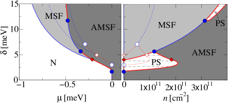
Figure 2: (Color online) $T=0$ phase diagram for a GaAs microcavity, plotting cavity-exciton detuning $\delta$ vs. chemical potential $\mu$ (left) or total density $n$ (right). The normal phase N is white, MSF shaded light- and AMSF is dark-grey. First (thick [red]) and second (thinner [blue]) order lines are separated by tricritical points ([blue] circles), while critical end-points are (red) diamonds. Horizontal dot-dashed lines connect the same chemical potential first-order boundaries in the phase separated (PS) region. Dashed lines are the mean-field boundaries neglecting quantum fluctuations.

Zero temperature —

Figure 2 shows the $T=0$ phase diagram for the GaAs parameters specified above. The axes are the detuning $\delta$ and either the chemical potential $\mu$ or the total density, $n=\sum_{{\mathbf{k}}}\langle\hat{a}_{{\mathbf{k}}\uparrow}^{{\dagger}}\hat{a}_{{\mathbf{k}}\uparrow}+\hat{a}_{{\mathbf{k}}\downarrow}^{{\dagger}}\hat{a}_{{\mathbf{k}}\downarrow}+2\hat{a}_{{\mathbf{k}}m}^{{\dagger}}\hat{a}_{{\mathbf{k}}m}\rangle/\mathcal{A}$. Details of the calculation appear below. Varying $\delta$ changes both the inter-channel detuning $\nu$ and the LP dispersion $\omega_{k}^{LP}$. Three phases exist : The normal phase (N), $\psi_{\uparrow}=\psi_{\downarrow}=\psi_{m}=0$ (where $\psi_{\sigma}=\langle\hat{\psi}_{\sigma}\rangle=\langle\hat{a}_{{\mathbf{k}}\sigma}\rangle\delta_{{\mathbf{k}},0}/\sqrt{\mathcal{A}}$) and two condensed phases arising from the spontaneous symmetry breaking of the $U(1)\times U(1)$ global symmetry, $\hat{\psi}_{\uparrow,\downarrow}\mapsto e^{i\phi_{\uparrow,\downarrow}}\hat{\psi}_{\uparrow,\downarrow}$, $\hat{\psi}_{m}\mapsto e^{i(\phi_{\uparrow}+\phi_{\downarrow})}\hat{\psi}_{m}$. Condensation of atoms, $\psi_{\uparrow}=\psi_{\downarrow}\neq 0$, guarantees that of molecules, $\psi_{m}\neq 0$ (but not vice-versa). We denote this phase as an atomic and molecular superfluid phase (AMSF): Here, the $U(1)\times U(1)$ symmetry is completely broken. The third phase is characterized by the absence of atomic ODLRO but where molecules do condense, the MSF phase Kuklov et al. (2004a, b); Radzihovsky et al. (2004); Romans et al. (2004); Radzihovsky et al. (2008). The MSF phase has a residual $U(1)$ symmetry (rotations with $\phi_{\uparrow}+\phi_{\downarrow}=\text{const}.$).

For $\delta\lesssim 1.6$ meV, Fig. 2 shows a second order N-AMSF transition, as expected when bipolaritons are irrelevant. As $\delta$ increases, $\nu$ decreases and the bare resonance occurs at $\delta=3.84$ meV. The MSF phase appears at slightly higher $\delta\simeq 4.0$ meV. This is because near the resonance — between the lower two tricritical points (solid [blue] circles) — the the N-AMSF phase transition becomes first order, leading to phase separation (right panel of Fig. 2), a dramatic signature of the resonance effects. Phase separation occurs either between N and AMSF below the critical end-point (solid [red] diamond at $\delta\simeq 4.0$ meV), or above, between MSF and AMSF. Above the second tricritical point, there is a second order N-MSF transition at $2\mu=\nu$, which is then followed by a second order MSF-AMSF transition. This MSF-AMSF transition occurs when the renormalized bipolariton energy (due to the interaction $\tilde{U}_{X}^{mm}$) reaches the polariton energy, as discussed in Basu and Mueller (2008). At even higher detunings, the MSF-AMSF transition becomes first order again, driven by the changing polariton dispersion, (see SM ).

As well as clear signatures in the form of the phase diagram, the different collective paired phases can be experimentally identified via spatial correlation functions. In particular, at $T=0$, the AMSF phase is characterized by ODLRO of both unpaired polaritons and bipolaritons. At $T\neq 0$, as the system is 2D, this evolves into off-diagonal quasi long-range order (ODqLRO), i.e., power-law decay of the correlation functions $g^{(1)}_{\uparrow,\downarrow}({\mathbf{r}})=\langle\hat{\psi}_{\uparrow,\downarrow}^{\dagger}({\mathbf{r}})\hat{\psi}_{\uparrow,\downarrow}(0)\rangle$ and $g^{(1)}_{m}({\mathbf{r}})=\langle\hat{\psi}_{\uparrow}^{\dagger}({\mathbf{r}})\hat{\psi}_{\downarrow}^{\dagger}({\mathbf{r}})\hat{\psi}_{\downarrow}(0)\hat{\psi}_{\uparrow}(0)\rangle$. In contrast, the MSF phase is characterized by the absence of any order for unpaired polaritons, but the power-law decay of $g^{(1)}_{m}({\mathbf{r}})$: The observation of such pair correlations without polariton correlations would provide unambiguous evidence for an MSF phase. An experimental scheme to measure $g^{(1)}_{m}$ is given in SM .

To derive the $T=0$ phase diagram we employ a variational approach, by considering a normalized Bogoliubov–Nozières ground state Nozières and Saint James (1982) including atomic and molecular condensates, as well as pairing terms:

$$|\psi\rangle=\mathcal{N}\exp\Bigg{(}\displaystyle\sqrt{\mathcal{A}}\sum_{\sigma=\uparrow,\downarrow,m}\psi_{\sigma}\hat{a}_{0\sigma}^{\dagger}\\ +\sum_{{\mathbf{k}}}\sum_{\gamma=a,b,m}\tanh\theta_{{\mathbf{k}}\gamma}\hat{b}_{{\mathbf{k}}\gamma}^{\dagger}\hat{b}_{-{\mathbf{k}}\gamma}^{\dagger}\Bigg{)}|0\rangle\;.$$

The operators $\hat{b}_{{\mathbf{k}}\gamma}$ are related to $\hat{a}_{{\mathbf{k}}\sigma}$ by:

$$\begin{pmatrix}\hat{a}_{{\mathbf{k}}\uparrow}^{{\dagger}}\\ \hat{a}_{{\mathbf{k}}\downarrow}^{\dagger}\end{pmatrix} =\displaystyle\frac{1}{\sqrt{2}}\begin{pmatrix}1&1\\ -1&1\end{pmatrix}\begin{pmatrix}\hat{b}_{{\mathbf{k}}a}^{{\dagger}}\\ \hat{b}_{{\mathbf{k}}b}^{\dagger}\end{pmatrix} \hat{a}_{{\mathbf{k}}m}^{{\dagger}} =\hat{b}_{{\mathbf{k}}m}^{{\dagger}}\;.$$

Note that $\sigma=\uparrow,\downarrow,m$, while $\gamma=a,b,m$. This transformation produces the most general ($\uparrow\leftrightarrow\downarrow$ symmetric) variational ground state including pairing. Minimizing the energy $\langle\hat{H}\rangle$ over the variational parameters $\psi_{\uparrow}=\psi_{\downarrow}=\psi_{0}$, $\psi_{m}$, and $\theta_{{\mathbf{k}}\gamma}$ we find that $\theta_{{\mathbf{k}}\gamma}$ has the functional form $\tanh 2\theta_{{\mathbf{k}}\gamma}={\alpha_{\gamma}}/{(\epsilon_{{\mathbf{k}}\gamma}+\beta_{\gamma})}$, with $\beta_{\gamma}>0,|\alpha_{\gamma}|\leq\beta_{\gamma}$, and $\epsilon_{{\mathbf{k}}a,b}=\omega_{{\mathbf{k}}}^{LP}-\omega_{0}^{LP}$. The energy can thus be numerically minimized in terms of eight variational parameters $\alpha_{\gamma},\beta_{\gamma}$, and $\psi_{\sigma}$, making it easy to determine first order phase boundaries, as well as to find cases where the global minimum energy is not an extremum (zero derivative), but instead occurs at $|\alpha_{\gamma}|=\beta_{\gamma}$.

As $\tilde{U}^{\sigma\sigma^{\prime}}\ll\tilde{U}^{\sigma\sigma^{\prime}}_{X}\sim 1$ fluctuation corrections to mean field (MF) theory should be small. At the same time, as bipolaritons have a much larger mass than LPs, bipolariton fluctuations give a non-negligible shift. The dashed lines and empty symbols in Fig. 2 show the MF predictions. Fluctuations do shift the phase boundaries, but the phase diagram topology qualitatively matches MF predictions Radzihovsky et al. (2008), except for the TCP at large detuning where the MSF-AMSF transition becomes first order again (see SM ). At MF level the two tricritical points are at $(\mu,\nu)=(0,\Delta^{LP}_{00}/(4\bar{U}))$ and $(-\Delta^{LP}_{00}/(2\bar{W}),-\Delta^{LP}_{00}[\bar{W}^{-1}+(8\bar{U})^{-1}])$ where $\bar{U}=\tilde{U}^{\uparrow\uparrow}+\tilde{U}^{\uparrow\downarrow}$ and $\bar{W}=[\tilde{U}^{mm}(\tilde{U}^{\uparrow\uparrow}+\tilde{U}^{\uparrow\downarrow})]^{1/2}$.

Finite temperature —

We have shown that, in GaAs, a polariton MSF phase can be found at $T=0$ for $\delta\gtrsim 4.0$ meV. However, to see if such a phase is readily accessible, we must determine its critical temperature. Since the closed channel mass is $m_{M}\simeq 2m_{X}$, the critical temperature is expected to be much lower than corresponding LP condensation temperatures.

In order to extend our results to finite temperature, we use variational mean-field theory (VMFT) Radzihovsky et al. (2008); Kleinert (1995), based on the inequality Feynman (1998) $\mathcal{F}=-k_{B}T\ln\operatorname{tr}e^{-\hat{H}/k_{B}T}\leq\mathcal{F}_{v\text{MF}}=\mathcal{F}_{\text{MF}}+\langle\hat{H}-\hat{H}_{\text{MF}}\rangle_{\text{MF}}$. In a similar spirit to the $T=0$ calculation, $\hat{H}_{\text{MF}}$ is chosen to allow the same one- and two-point correlation functions and its variational parameters are used to minimize $\mathcal{F}_{v\text{MF}}$:

$$\hat{H}_{\text{MF}}=\sum_{\gamma}\Bigg{\{}-\sqrt{\mathcal{A}}\psi_{\gamma}\left(\alpha_{\gamma}+\beta_{\gamma}\right)\left(\hat{b}_{0\gamma}^{\dagger}+\hat{b}_{0\gamma}\right)\\ +\displaystyle\frac{1}{2}\sum_{{\mathbf{k}}}\begin{pmatrix}\hat{b}_{{\mathbf{k}}\gamma}^{\dagger}&\hat{b}_{-{\mathbf{k}}\gamma}\end{pmatrix}\begin{pmatrix}\epsilon_{{\mathbf{k}}\gamma}+\beta_{\gamma}&\alpha_{\gamma}\\ \alpha_{\gamma}&\epsilon_{{\mathbf{k}}\gamma}+\beta_{\gamma}\end{pmatrix}\begin{pmatrix}\hat{b}_{{\mathbf{k}}\gamma}\\ \hat{b}_{-{\mathbf{k}}\gamma}^{\dagger}\end{pmatrix}\Bigg{\}}\;,$$

where $\psi_{a}=0$ and $\psi_{b}=\sqrt{2}\psi_{0}$. As before, the functional form of the matrix elements above is the optimal form. We evaluate $\mathcal{F}_{\text{MF}}$ and averages $\langle\ldots\rangle_{\text{MF}}$ by standard Bogoliubov diagonalization Pitaevskii and Stringari (2003). This yields the free energy $\mathcal{F}_{v\text{MF}}$ as a function of the same eight parameters $\alpha_{\gamma}$, $\beta_{\gamma}$, and $\psi_{0},\psi_{m}$, again allowing numerical minimization. Note that the $T=0$ limit of this approach reproduces the results presented above.

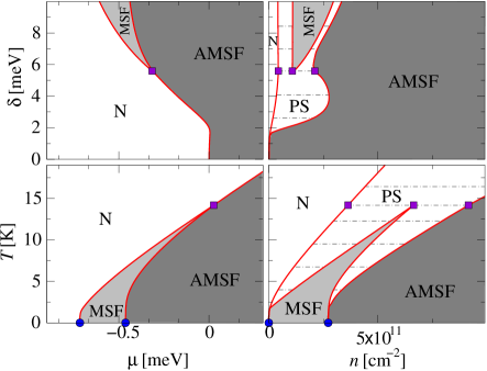
Figure 3: (Color online) Finite temperature phase diagrams with the same notation, color scheme and GaAs parameters as in Fig. 2. The critical end-point of Fig. 2 is now replaced by a triple point ([purple] square). Temperature is fixed to $T=4$ K ($k_{B}T=0.34$ meV) in the top panels, while detuning is $\delta=10$ meV in the bottom ones.

For 2D Bose gases the actual $T\neq 0$ transition to a superfluid phase is of the Berezinskii-Kosterlitz-Thouless (BKT) type Pitaevskii and Stringari (2003). Instead, VMFT predicts a first order transition. The N-AMSF and MSF-AMSF transitions can be very weakly first order due to the small polariton mass SM . Despite the absence of true ODLRO, the quasi-condensate density plays a similar role to the mean-field order parameter Kagan et al. (2000); Prokof’ev and Svistunov (2002). This allows Hartree-Fock Popov (1983); Pitaevskii and Stringari (2003) or equivalent approaches (such as VMFT) to reproduce the equation of state of the system outside of the critical region. As such, the location of phase boundaries predicted by VMFT should be accurate, and we have verified this for the homonuclear weakly interacting 2D Bose gas by comparison to the Monte-Carlo results of Prokof’ev and Svistunov (2002). In the 3D homonuclear case, other approaches such as applications of the Nozières-Schmitt-Rink approximation Nozieres and Schmitt-Rink (1985) have been considered, predicting only second order transitions Koetsier et al. (2009).

Figure 3 shows the phase diagram both vs $\delta$ at fixed $T$ (top panels) and vs $T$ at fixed $\delta$ (bottom panels). The main new features introduced by non-zero temperature are the existence of a non-zero critical density for the normal state and the extension to arbitrarily large detuning of the phase separated region as discussed above. Because the N-MSF transition is now first order, the critical end-point at $T=0$ is replaced by a triple point. At yet higher temperatures, the triple point moves to higher $\delta$ and eventually merges with the tricritical point (see SM ). In the phase diagram vs temperature at $\delta=10$ meV, one sees that the MSF phase survives up to $T\sim 14.2$ K ($1.28$ meV). For ZnO Li et al. (2013) the MSF phase can survives to higher temperatures and lower detunings SM .

Conclusions

To conclude, we argue that microcavity polaritons are an ideal system to explore collective pairing phases of bosons. In particular, in addition to the standard polariton superfluid phase, where both polaritons and bipolaritons are characterized by off-diagonal quasi long-range order, we highlight a new phase which displays molecular superfluidity (MSF), i.e., order for bipolaritons but not for polaritons. This phase covers an increasing region of the phase diagram at either larger cavity-exciton detunings or lower temperatures. While for the GaAs parameters considered here we predict the MSF phase to survive up to $T\sim 14$ K at a cavity-exciton detuning $\delta=10$ meV, this temperature can be higher for materials with larger Rabi splitting, such as ZnO.

I Model parameters

Our manuscript calculates the phase diagram of the polariton system using the two-channel model, given in Eq. (1) of the manuscript. This model describes the interacting lower polariton (LP) fields in the two circular polarization states $\hat{\psi}_{\uparrow,\downarrow}({\mathbf{r}})=[\hat{\psi}_{x}({\mathbf{r}})\pm i\hat{\psi}_{y}({\mathbf{r}})]/\sqrt{2}$ ($x,y$ are the linear polarization components) and the bipolariton $\hat{\psi}_{m}({\mathbf{r}})$ field. Such a model is the low-energy effective theory of a more complicated model of interacting excitons strongly coupled to photons. Most properties of the bipolariton field in our model are the same as those of pure biexcitons, although the bipolariton does contain a small photon component. This small photon component provides crucial distinctions from a pure biexciton state. In particular, the photon component ensures that optically active states are the lowest in energy.

To clarify these points, we give here a short account of the derivation of the effective polariton and bipolariton parameters appearing in the two-channel model, such as the effective interaction strengths $U^{\sigma\sigma^{\prime}}_{{\mathbf{k}}{\mathbf{k}^{\prime}}{\mathbf{q}}}$ (where $\sigma,\sigma^{\prime}=\uparrow,\downarrow,m$) and the Feshbach resonance coupling $g_{{\mathbf{k}}{\mathbf{Q}}}$, the inter-channel detuning $\nu$, the bipolariton mass $m_{m}$, and their dependence on the exciton-photon detuning $\delta=\omega_{0}^{C}-\omega_{0}^{X}$, where $\omega_{{\mathbf{k}}}^{C,X}$ are the photon and exciton energies. Changing the detuning $\delta$ changes the LP composition, and hence affects the polariton dispersion, its scattering properties, and the overlap with the biexciton states. Many of these results are also reported in the manuscript, for completeness we include all relevant formulae here.

The LP dispersion $\omega_{{\mathbf{k}}}^{LP}$ has the form $2\omega_{{\mathbf{k}}}^{LP}=\omega_{{\mathbf{k}}}^{C}+\omega_{{\mathbf{k}}}^{X}-\sqrt{(\omega_{{\mathbf{k}}}^{C}-\omega_{{\mathbf{k}}}^{X})^{2}+\Omega_{R}^{2}}$, as given in (and shown in Fig. 1 of) the manuscript. The non-quadratic form of this dispersion results from the varying composition of the LP, as determined by the Hopfield coefficients, $2c_{{\mathbf{k}}}^{2},2s_{{\mathbf{k}}}^{2}=1\pm(\omega_{{\mathbf{k}}}^{C}-\omega_{{\mathbf{k}}}^{X})/\sqrt{(\omega_{{\mathbf{k}}}^{C}-\omega_{{\mathbf{k}}}^{X})^{2}+\Omega_{R}^{2}}$, which give the exciton and photon fraction of the lower polariton at a given momentum ${\mathbf{k}}$.

In order to derive the appropriate dimensionless parameters characterizing the interaction strengths, it is necessary to identify an effective mass of the LP. This corresponds to the expansion at small ${\mathbf{k}}$, $\omega_{{\mathbf{k}}}^{LP}-\omega_{0}^{LP}\simeq k^{2}/2m$, where $m=m_{LP}({\mathbf{k}}=0)$. This polariton mass is given by

$$\frac{m}{m_{X}}=\frac{1}{c_{0}^{2}+s_{0}^{2}m_{X}/m_{C}}\;,$$ (1)

where the Hopfield coefficients at ${\mathbf{k}}=0$ take a simple form:

$$c_{0}^{2},s_{0}^{2}=\displaystyle\frac{1}{2}\left[1\pm\displaystyle\frac{\delta}{\sqrt{\delta^{2}+\Omega_{R}^{2}}}\right].$$ (2)

We will discuss what changes would occur if this quadratic approximation of the LP dispersion were used in calculating the phase diagram; in particular, in Sec. III, we will compare these results with those obtained in the manuscript by making use of the full LP dispersion.

From the LP dispersion, we can also express the detuning between closed and open channels (the inter-channel detuning), $\nu=-|E_{b}|-2[\omega_{0}^{LP}-\omega_{0}^{X}]$, in terms of the exciton-photon detuning $\delta$:

$$\nu=-|E_{b}|-\delta+\sqrt{\delta^{2}+\Omega_{R}^{2}}\;.$$ (3)

A plot of the dependence of $\nu$ and $m/m_{X}$ on the detuning $\delta$ for typical GaAs parameters can be found in the manuscript Fig. 1(c).

The background polariton interaction strengths $U^{\uparrow\uparrow}=U^{\downarrow\downarrow}$, $2U^{\uparrow\downarrow}$ can be written in terms of the corresponding excitonic interaction strengths. They depend on the polariton or exciton mass used to define dimensionless interaction constants $\tilde{U}^{\sigma\sigma^{\prime}}$ and $\tilde{U}^{\sigma\sigma^{\prime}}_{X}$, as well as on the excitonic fraction, i.e., the Hopfield coefficient $c_{{\mathbf{k}}}$, which introduces a non-trivial dependence of the polariton interaction strengths on the momentum ($\hbar=1$):

$$U_{{\mathbf{k}}{\mathbf{k}}^{\prime}{\mathbf{q}}}^{\sigma\sigma^{\prime}}=\frac{\tilde{U}_{{\mathbf{k}}{\mathbf{k}}^{\prime}{\mathbf{q}}}^{\sigma\sigma^{\prime}}}{m}=c_{{\mathbf{k}}}c_{{\mathbf{k}}^{\prime}}c_{{\mathbf{k}}^{\prime}-\frac{{\mathbf{q}}}{2}}c_{{\mathbf{k}}+\frac{{\mathbf{q}}}{2}}\frac{\tilde{U}^{\sigma\sigma^{\prime}}_{X}}{m_{X}}\;,$$ (4)

where $\sigma,\sigma^{\prime}$ run over $\uparrow,\downarrow$ only here. The background bipolariton interaction $U^{mm}$ does not involve the polariton Hopfield coefficients because, as we will see below, the bipolariton is strongly excitonic regardless of momentum.

The hybridization (coupling) $g_{{\mathbf{k}}{\mathbf{Q}}}$ between pairs of LPs in opposite polarizations and bipolaritons, as well as the bipolariton mass $m_{m}$, can be estimated from the expression for the LP-LP scattering $T$-matrix, $t_{LPLP}(E,{\mathbf{k}},{\mathbf{k}}^{\prime},{\mathbf{Q}})$. The bipolariton appears as a scattering resonance in this $T$-matrix, and its mass depends on the dispersion of that resonance. The $T$-matrix can be evaluated starting from the $T$-matrix for two excitons in opposite polarizations, $t_{XX}(E,{\mathbf{k}},{\mathbf{k}}^{\prime},{\mathbf{Q}})$, scattering from momenta $({\mathbf{k}}+{\mathbf{Q}}/2,-{\mathbf{k}}+{\mathbf{Q}}/2)$ to momenta $({\mathbf{k}}^{\prime}+{\mathbf{Q}}/2,-{\mathbf{k}}^{\prime}+{\mathbf{Q}}/2)$. Assuming that the exciton scattering is dominated by the biexciton resonance, one can assume the following simplified expression for $t_{XX}(E,{\mathbf{k}},{\mathbf{k}}^{\prime},{\mathbf{Q}})$:

$$t_{XX}(E,{\mathbf{k}},{\mathbf{k}}^{\prime},{\mathbf{Q}})\simeq\frac{4\pi}{m_{X}}\displaystyle\frac{\Delta^{X}}{E-\omega_{XX}-\frac{Q^{2}}{2(2m_{X})}}\;.$$ (5)

We then include the exciton-photon coupling to evaluate $t_{LPLP}(E,{\mathbf{k}},{\mathbf{k}}^{\prime},{\mathbf{Q}})$. Using the results of Ref. Wouters (2007), one has that

$$t_{LPLP}(E,{\mathbf{k}},{\mathbf{k}}^{\prime},{\mathbf{Q}})=\displaystyle\frac{c_{{\mathbf{k}}+\frac{{\mathbf{Q}}}{2}}c_{-{\mathbf{k}}+\frac{{\mathbf{Q}}}{2}}c_{{\mathbf{k}}^{\prime}+\frac{{\mathbf{Q}}}{2}}c_{-{\mathbf{k}}^{\prime}+\frac{{\mathbf{Q}}}{2}}}{t_{XX}^{-1}(E,{\mathbf{k}},{\mathbf{k}}^{\prime},{\mathbf{Q}})-D(E,{\mathbf{Q}})}\;,$$ (6)

where

$$D(E,{\mathbf{Q}})=\sum_{{\mathbf{p}}}\left[\displaystyle\frac{c_{{\mathbf{p}}}^{2}c_{-{\mathbf{p}}+{\mathbf{Q}}}^{2}}{E-\omega_{{\mathbf{p}}}^{LP}-\omega_{-{\mathbf{p}}+{\mathbf{Q}}}^{LP}}-\displaystyle\frac{1}{E-2\omega_{{\mathbf{p}}}^{X}}\right.\\ \left.+\displaystyle\frac{2c_{{\mathbf{p}}}^{2}s_{-{\mathbf{p}}+{\mathbf{Q}}}^{2}}{E-\omega_{{\mathbf{p}}}^{LP}-\omega_{-{\mathbf{p}}+{\mathbf{Q}}}^{UP}}+\displaystyle\frac{s_{{\mathbf{p}}}^{2}s_{-{\mathbf{p}}+{\mathbf{Q}}}^{2}}{E-\omega_{{\mathbf{p}}}^{UP}-\omega_{-{\mathbf{p}}+{\mathbf{Q}}}^{UP}}\right]\;,$$ (7)

and where the dispersion of the upper polariton (UP) is $2\omega_{{\mathbf{k}}}^{UP}=\omega_{{\mathbf{k}}}^{C}+\omega_{{\mathbf{k}}}^{X}+\sqrt{(\omega_{{\mathbf{k}}}^{C}-\omega_{{\mathbf{k}}}^{X})^{2}+\Omega_{R}^{2}}$. The propagator $D(E,{\mathbf{Q}})$ is generally a smooth function of the energy $E$, except at isolated points. For zero center of mass momentum, ${\mathbf{Q}}=0$, these isolated points, where it diverges logarithmically, occur near the 2-particle band-edge energies (i.e., $E\sim 2\omega_{0}^{LP}$, $E\sim\omega_{0}^{LP}+\omega_{0}^{UP}$, and $E\sim 2\omega_{0}^{UP}$). Because $m_{C}\ll m_{X}$, the ratio between polariton and exciton mass $m/m_{X}$ also generally satisfies $m/m_{X}\ll 1$, unless at very large detuning $\delta\gg\Omega_{R}$ (see manuscript Fig. 1(c)). The existence of this small parameter suppresses the renormalization term $D(E,{\mathbf{Q}})$. In general it causes only a small shift of the resonance energy away from $\omega_{XX}+\frac{Q^{2}}{2(2m_{X})}$, thus giving:

$$t_{LPLP}(E,{\mathbf{k}},{\mathbf{k}}^{\prime},{\mathbf{Q}}) \simeq\frac{4\pi}{m}\displaystyle\frac{g_{{\mathbf{k}}{\mathbf{Q}}}g_{{\mathbf{k}}^{\prime}{\mathbf{Q}}}m}{E-\omega_{XX}-\frac{Q^{2}}{2(2m_{X})}},$$ (8)

$$g_{{\mathbf{k}}{\mathbf{Q}}} =c_{{\mathbf{k}}+\frac{{\mathbf{Q}}}{2}}c_{-{\mathbf{k}}+\frac{{\mathbf{Q}}}{2}}\sqrt{\Delta^{X}/m_{X}}.$$ (9)

The Feshbach coupling $g_{{\mathbf{k}}{\mathbf{Q}}}$ is related to the resonance width $\Delta^{LP}_{{\mathbf{k}}{\mathbf{Q}}}$ by $\Delta^{LP}_{{\mathbf{k}}{\mathbf{Q}}}=mg_{{\mathbf{k}}{\mathbf{Q}}}^{2}$ Gurarie and Radzihovsky (2007), so that

$$\Delta^{LP}_{{\mathbf{k}}{\mathbf{Q}}}=c_{{\mathbf{k}}+\frac{{\mathbf{Q}}}{2}}^{2}c_{-{\mathbf{k}}+\frac{{\mathbf{Q}}}{2}}^{2}\Delta^{X}\displaystyle\frac{m}{m_{X}}\;.$$ (10)

We have verified that, for the system parameters relevant for current experiments in GaAs (see later section “GaAs parameters”), the above approximation,

$$g^{2}_{{\mathbf{k}}{\mathbf{Q}}}\simeq c_{{\mathbf{k}}+\frac{{\mathbf{Q}}}{2}}^{2}c_{-{\mathbf{k}}+\frac{{\mathbf{Q}}}{2}}^{2}\Delta^{X}/m_{X}\;,$$ (11)

is accurate up to $\delta\lesssim 33$ meV, and $0.1$ meV away from the resonance (i.e., $\nu=0$ which corresponds to $\delta=3.84$ meV), with an error below $5\%$, in the limit ${\mathbf{k}}\to 0$ and ${\mathbf{Q}}\to 0$.

Thus we have seen that most properties of bipolaritons are the same as those of pure biexcitons. However, even when the photon fraction is very small, the photon component has crucial effects. Firstly, given the small ratio, $m_{C}/m_{X}=10^{-4}$, even a 1% photon fraction reduces the polariton mass $m$ by two orders of magnitude compared to the bare excitonic mass. As such, a 99% excitonic polariton system can behave quite distinctly from a pure excitonic system Li et al. (2013); Trichet et al. (2013). In addition to the change of mass (relevant for when later we will make use of the quadratic approximation of the LP dispersion) there is another significant effect on excitons when including a small mixing with photons. In GaAs, excitons can have angular momentum $J_{z}=\pm 2,\pm 1$. These states are almost degenerate, with a weak (typically a few $\mu$eV van Kesteren et al. (1990)) electron-hole exchange term favoring the “dark” $J_{z}=\pm 2$ states Combescot et al. (2007). Photons couple only to the optically active “bright” state $J_{z}=\pm 1$ thus lower the energy of these states. If the Rabi splitting is typically $10^{3}$ times larger than the exchange splitting, i.e. a few meV rather than a few $\mu$eV, then only 0.1% photon fraction is required to overcome the exchange splitting. Thus, while the ground state of a pure excitonic system is expected to be dark, the ground state of 99.9% excitonic system is likely bright Li et al. (2013); Trichet et al. (2013). Such photon induced splitting of bright and dark states can also be important for the bipolariton, even when the bipolariton mass and energy are very similar to those of the biexciton.

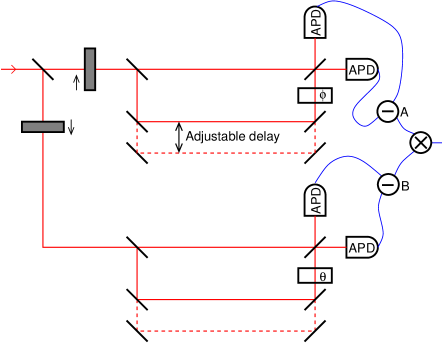
S. Fig. 1: Schematic optical detection setup for measuring time-dependent pair correlations $g^{(1)}_{m}(0,t)$.

II Detection of pairing correlations

In the manuscript we discussed the distinct signatures for detecting the MSF and AMSF phases. The clearest signature is that the MSF phase would show pair coherence, but no polariton coherence. Experiments to determine whether polariton coherence exists, by measuring $g^{(1)}_{\sigma}({\mathbf{r}},t)=\langle\hat{\psi}_{\sigma}^{\dagger}({\mathbf{r}},t)\hat{\psi}_{\sigma}(0,0)\rangle$ are routine and can be extracted from interference fringe visibility maps between two images of the condensate. Measuring such correlations clearly distinguishes the AMSF phase from the MSF or Normal phase. However, to unambiguously distinguish between the normal and the MSF phases it is necessary instead to measure the following molecular first order correlation function $g^{(1)}_{m}({\mathbf{r}},t)=\langle\hat{\psi}_{\uparrow}^{\dagger}({\mathbf{r}},t)\hat{\psi}_{\downarrow}^{\dagger}({\mathbf{r}},t)\hat{\psi}_{\downarrow}(0,0)\hat{\psi}_{\uparrow}(0,0)\rangle$. In this section we present one possible scheme to measure $g^{(1)}_{m}(0,t)$; a similar setup with spatial resolution could be used to measure $g^{(1)}_{m}({\mathbf{r}},t)$. Other possible schemes to measure these quantities are possible, our aim here is to illustrate the possibility of such measurements.

Supplemental Figure 1 shows a possible experimental scheme that measures the pair correlations $g^{(1)}_{m}(0,t)$. The scheme is based on cross-correlation measurements between a pair of balanced homodyne detectors, which separately measure two-time correlations of the different polarization states. Light from the sample is split on an initial beamsplitter and filtered into the two circular polarization components, $\uparrow$ and $\downarrow$. This light is then sent through a variable delay interferometer, with an adjustable phase shift $\phi$ for $\uparrow$ polarization ($\theta$ for $\downarrow$ polarization). The same delay is used for both the $\uparrow$ and $\downarrow$ branches of the apparatus. The light is then measured via a balanced homodyne scheme, so that at $A$ the output is:

$$I_{A} =\frac{1}{2}\langle[\hat{\psi}^{\dagger}_{\uparrow}(t)-ie^{-i\phi}\hat{\psi}^{\dagger}_{\uparrow}(t^{\prime})][\hat{\psi}_{\uparrow}(t)+ie^{i\phi}\hat{\psi}_{\uparrow}(t^{\prime})]\rangle$$

$$-\frac{1}{2}\langle[-i\hat{\psi}^{\dagger}_{\uparrow}(t)+e^{-i\phi}\hat{\psi}^{\dagger}_{\uparrow}(t^{\prime})][i\hat{\psi}_{\uparrow}(t)+e^{i\phi}\hat{\psi}_{\uparrow}(t^{\prime})]\rangle$$

$$=ie^{i\phi}\langle\hat{\psi}^{\dagger}_{\uparrow}(t)\hat{\psi}_{\uparrow}(t^{\prime})\rangle+\text{h.c.}\;,$$

where $t^{\prime}=t+\tau$, $\tau$ is the adjustable delay, and $\phi$ the phase shift. This signal on its own averages to zero in the MSF phase as there is no single polariton phase coherence. A similar form applies for the lower branch of the interferometer $B$ with $\uparrow\mapsto\downarrow$ and $\phi\mapsto\theta$. When calculating the cross correlation $I_{\text{out}}=\langle I_{A}\times I_{B}\rangle$, one therefore obtains a signal:

$$I_{\text{out}}= -e^{i(\phi+\theta)}\langle\hat{\psi}^{\dagger}_{\uparrow}(t)\hat{\psi}_{\uparrow}(t^{\prime})\hat{\psi}^{\dagger}_{\downarrow}(t)\hat{\psi}_{\downarrow}(t^{\prime})\rangle$$

$$+e^{i(\phi-\theta)}\langle\hat{\psi}^{\dagger}_{\uparrow}(t)\hat{\psi}_{\uparrow}(t^{\prime})\hat{\psi}^{\dagger}_{\downarrow}(t^{\prime})\hat{\psi}_{\downarrow}(t)\rangle$$

$$+e^{i(\theta-\phi)}\langle\hat{\psi}^{\dagger}_{\uparrow}(t^{\prime})\hat{\psi}_{\uparrow}(t)\hat{\psi}^{\dagger}_{\downarrow}(t)\hat{\psi}_{\downarrow}(t^{\prime})\rangle$$

$$-e^{-i(\phi+\theta)}\langle\hat{\psi}^{\dagger}_{\uparrow}(t^{\prime})\hat{\psi}_{\uparrow}(t)\hat{\psi}^{\dagger}_{\downarrow}(t^{\prime})\hat{\psi}_{\downarrow}(t)\rangle\;.$$ (12)

In the absence of a symmetry breaking magnetic field, correlations should be invariant under the replacement $\uparrow\leftrightarrow\downarrow$ and so the middle two lines involve the same expectation. Choosing $\phi-\theta=\pi/2$ then means these middle two lines vanish. Choosing also $\phi+\theta=\pi$, so that $\phi=3\pi/4,\theta=\pi/4$, the first and last lines have the same prefactor giving:

$$I_{\text{out}} =\langle\hat{\psi}^{\dagger}_{\uparrow}(t)\hat{\psi}_{\uparrow}(t^{\prime})\hat{\psi}^{\dagger}_{\downarrow}(t)\hat{\psi}_{\downarrow}(t^{\prime})\rangle$$

$$+\langle\hat{\psi}^{\dagger}_{\uparrow}(t^{\prime})\hat{\psi}_{\uparrow}(t)\hat{\psi}^{\dagger}_{\downarrow}(t^{\prime})\hat{\psi}_{\downarrow}(t)\rangle\;.$$ (13)

In the steady state, this implies that $I_{\text{out}}\propto g_{m}^{(1)}(0,\tau)+g_{m}^{(1)}(0,-\tau)$, and as the coherent part of the two-time correlation function should be symmetric in $\tau$, such a scheme allows measurement of the pair coherence.

III Comparing the case of full LP dispersion with the quadratic approximation limit

In the manuscript we always use the full LP dispersion $\omega^{LP}_{{\mathbf{k}}}$. It is however instructive to compare this to the quadratic approximation $\omega_{{\mathbf{k}}}^{LP}-\omega_{0}^{LP}\simeq k^{2}/2m$ discussed above. This approximation corresponds to assuming that the occupation of the low-momentum polariton states dominates all relevant expectations values, and so in this limit it is consistent to also replace all Hopfield factors with $c_{{\mathbf{k}}},s_{{\mathbf{k}}}\to c_{0},s_{0}$.

Approximating the LP dispersion by its low-momentum expansion is expected to be accurate in the limit when fluctuations beyond mean-field are small: The mean-field results do not depend on the polariton dispersion at all, since they involve only the ${\mathbf{k}}=0$ fields. As discussed in the manuscript, in the photonic limit the small polariton mass $m\ll m_{X}$ suppresses fluctuations, however at large $\delta$, fluctuations are significant, and the full dispersion yields different predictions. Nonetheless, all the qualitative features of the phase diagrams obtained by using the full LP dispersion can be explained also by considering the quadratic approximation.

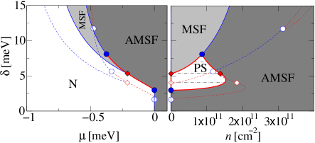
S. Fig. 2: Comparison between the phase diagrams at $T=0$ in the quadratic approximation $\omega_{{\mathbf{k}}}^{LP}-\omega_{0}^{LP}\simeq k^{2}/2m$ (solid lines), and with the full LP dispersion $\omega_{{\mathbf{k}}}^{LP}$ (dashed lines). The latter correspond to the boundaries shown in the Fig. 2 of the manuscript. Notation and color scheme are the same as in the manuscript.

We plot in S. Fig. 2 the comparison between the phase diagram at $T=0$ in the quadratic approximation, and with the full dispersion. The basic topology is qualitatively the same, with the difference that in the quadratic approximation the MSF-AMSF phase separation re-emerges only at very large $\delta$ compared with the case of the full LP dispersion. This can also be seen more clearly in S. Fig. 3 which shows the results of the quadratic approximation, but choosing a “heavier” cavity photon mass, $m_{C}=10^{-3}m_{X}$. This demonstrates that this feature is not dependent on the non-quadratic dispersion, but arises whenever the polariton density of states becomes very large, as occurs at large detunings. This in turn leads to a fluctuation dominated regime, which can drive the phase boundary first order. Since the full LP dispersion becomes strongly excitonic at large momentum, this generally increases the polariton density of states as compared to the quadratic approximation, enhancing such an effect.

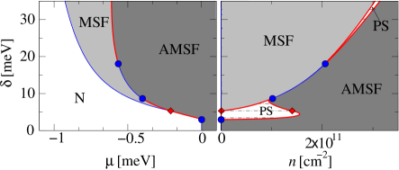
S. Fig. 3: Zero temperature phase diagram calculated in the quadratic approximation, but choosing an artificially large cavity photon mass $m_{C}/m_{X}=10^{-3}$. This shows that the phase separation occurring at large $\delta$ is not specific to the non-quadratic polariton dispersion.

In a similar way, other apparent differences between the quadratic approximation and the full dispersion cases arising at finite temperature can also be shown to be reproduced in the quadratic approximation with heavier photons. For example, the phase diagram at $\delta=10$K shown in Fig. 3 of the manuscript, and S. Fig. 6 appears to behave differently at low temperature. The behavior of the full dispersion is however closely replicated by the quadratic approximation if one takes $m_{C}/m_{X}=10^{-2}$, as shown in S. Fig. 4. This confirms the statement that while the full dispersion introduces important quantitative changes, no qualitatively new behavior occurs due to the full dispersion.

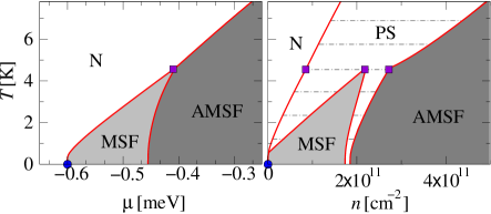
S. Fig. 4: Finite temperature phase diagram at fixed exciton-photon detuning $\delta=10$ meV, calculated in the quadratic approximation but taking artificially large cavity photon mass $m_{C}/m_{X}=10^{-2}$. This is qualitatively similar to the behavior seen in Fig. 3 of the manuscript.

The use of the quadratic approximation has the advantage to allowing significantly faster determination of the phase boundaries in our variational approach. The variational approach requires finding the free energy for each value of the variational parameters, and this requires estimating the integrals $\int d{\mathbf{k}}\langle a^{\dagger}_{{\mathbf{k}}\sigma}a_{{\mathbf{k}}\sigma^{\prime}}\rangle$ and $\int d{\mathbf{k}}\langle a_{{\mathbf{k}}\sigma}a_{{\mathbf{k}}\sigma^{\prime}}\rangle$. Within the quadratic approximation, these integrals are almost all analytic. This significant speedup allows a more comprehensive study of the three dimensional phase diagram (temperature $T$, detuning $\delta$ versus either density $n$ or detuning $\mu$), for which the full dispersion would be prohibitively computationally expensive. As such, the remainder of this supplemental material presents a comprehensive set of phase diagrams calculated in the quadratic approximation.

IV Quadratic approximation: Evolution of phase diagram with temperature and detuning

In the manuscript we presented several cuts through the three-dimensional phase diagram as a function of temperature, detuning and density (or chemical potential) for parameters relevant to GaAs. These cuts illustrate the main features that can be seen, namely the sequence of N-MSF-AMSF transitions and the direct N-AMSF transition; the existence of a first order transition and the associated phase separation (PS) near resonance at all temperatures, and the temperature dependence of the various phase boundaries. In this section we provide further cuts to illustrate more fully how the shape of the phase diagram evolves with changing detuning and temperature. Below we first present further figures illustrating the behavior for the system parameters which are relevant for GaAs microcavities. Then we compare the form of the phase diagram for GaAs parameters with that for ZnO parameters.

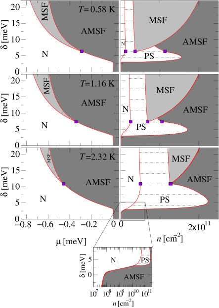
S. Fig. 5: Finite temperature phase diagrams for GaAs parameters in the low-momentum quadratic approximation for the LP dispersion plotted as a function of detuning $\delta$ for three different fixed temperatures ($T=0.58$ K, $T=1.16$ K, and $T=2.32$ K). Notation and color scheme are the same as those in the manuscript Fig. 3. For the last panel, corresponding to $T=2.32$ K, we also show the behavior of the N-PS-AMSF weakly first order boundary at low density and for negative detuning $\delta$ (please note the log-scale in density). As also discussed below, the behavior of the N-PS-AMSF first order transition for large and negative detunings $\delta$ follows the BKT scaling $T\sim n/m$, where $m$ is the LP mass. Thus, at fixed temperature, it exists a small, but finite, critical density for the N-PS-AMSF transition which is around $4$ order of magnitudes smaller than the critical density for the N-PS-MSF transition at positive and large detunings (which follows $T\sim n/m_{m}$).

IV.1 GaAs parameters

For GaAs, we fix the photon mass to $m_{C}=10^{-4}m_{X}$, the exciton mass $m_{X}=0.4m_{e}$, the Rabi splitting $\Omega_{R}=4.4$ meV, the biexciton binding energy $|E_{b}|=2$ meV, and the excitonic resonance width $\Delta^{X}=4|E_{b}|$ Wouters (2007). Additionally, $\tilde{U}^{\uparrow\uparrow}_{X}=\tilde{U}^{\downarrow\downarrow}_{X}=6$ Wouters (2007) and we also fix $\tilde{U}^{\uparrow\downarrow}_{X}=0$ and $\tilde{U}^{mm}_{X}=4$. Additional cuts through the phase diagram to those provided in the manuscript are here given in S. Figs. 5 and 6. These show cuts at various fixed temperatures (S. Fig. 5) or fixed detunings (S. Fig. 6).

The zero temperature phase diagram (see manuscript Fig. 2) is characterized by phase boundaries that are mostly second order, with a limited region in detuning near the resonance where the transition either between MSF-AMSF or N-AMSF is first order, thus implying phase separation (PS) for a range of densities. However, as S. Fig. 5 and S. Fig. 6 clearly show, at any non-zero temperature, all phase boundaries that were second order at zero temperature, evolve at finite temperature to weakly first order — as calculated within variational mean-field theory (VMFT). This is because, as discussed in the manuscript, at finite temperature, the real phase transitions are of the Berezinskii-Kosterlitz-Thouless type, involving a jump in the superfluid density, and VMFT approximates this by a weakly first order transition. The size of the jump depends on the mass of the condensing boson, and so the N-AMSF or MSF-AMSF transitions (determined by the polariton mass) show a very small jump. This density jump at the MSF-AMSF is just visible in the cut at $T=2.32$ K in S. Fig. 5, and is more pronounced in the manuscript Fig. 3 top panel where $T=4$ K. In the lower temperature cuts in S. Fig. 5 the jump is hardly visible. In contrast the jump at the N-MSF transition controlled by the biexciton mass $m_{m}=2m_{X}$, and is hence much larger, and so is clearly visible at all temperature in S. Fig. 5. Note also that, at large and negative detuning, the N-AMSF transition follows the BKT scaling $T\sim n/m$, where $m$ is the LP mass, while at large and positive detuning, the N-MSF transition follows $T\sim n/m_{m}$ and it depends on the biexciton mass $m_{m}=2m_{X}$. In particular, the AMSF region at large and negative detuning extends down up to a critical finite density (at finite temperature), as it is clearly shown in the low-density magnification of the bottom panel ($T=2.32$ K) of S. Fig. 5.

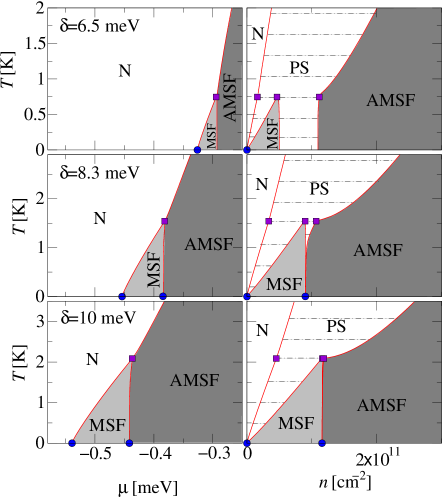
S. Fig. 6: Finite temperature phase diagrams for GaAs parameters in the low-momentum quadratic approximation for the LP dispersion plotted as a function of temperature $T$ for three different fixed exciton-photon detunings ($\delta=6.5$ meV, $\delta=8.3$ meV, and $\delta=10$ meV). Notation and color scheme are the same as the manuscript Fig. 3.

Since all phase boundaries are (at least weakly) first order, there are no true tricritical points, however the cuts at $T=0.58$ K and $T=1.16$ K show a remnant of the $T=0$ tricritical points (where the N-AMSF transition changes order near $\delta\simeq 3$ meV, and where the MSF-AMSF transition changes order near $\delta\simeq 7$ meV). At such points the finite temperature transition switches from being very weakly first order (controlled by the polariton mass) to being strongly first order, due to the resonance. As the temperature increases, while the lower “tricritical point” does not change substantially, the triple point approaches the upper “tricritical point”, so that, for $T\simeq 2.32$ K, the “tricritical point” and triple point have merged, as seen in the bottom panel of the S. Fig. 5.

The cuts at fixed $\delta$ in S. Fig. 6 show the same evolution that we have just described at fixed $T$. The size of jump in density at the AMSF-MSF transition is determined by whether the detuning is above or below the $T=0$ tricritical point. At $\delta=6.5$ meV (which, at $T=0$, is in between the critical end-point and the upper tricritical point), there is a first order transition between MSF-AMSF even at zero temperature. The panel at $\delta=8.3$ meV is very close to (and slightly above) the $T=0$ upper tricritical point, so the MSF-AMSF transition is second order at zero temperature and evolves to strongly first order at higher temperatures. Finally, for $\delta=10$ meV, the zero temperature transition is second order and becomes (weakly) first order at non-zero temperature.

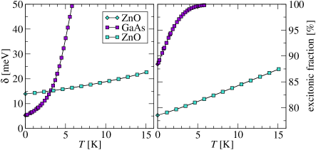
S. Fig. 7: Location of the triple points as a function of temperature for GaAs and ZnO parameters in the low-momentum quadratic approximation for the LP dispersion — note that at $T=0$ the triple points (squares) evolves into a critical end-point (diamond). Left panel: required detuning. Right panel: equivalent excitonic fraction.

IV.2 Evolution of triple point

The finite temperature phase diagrams presented above indicate that the MSF region shrinks on either reducing the detuning $\delta$ or on increasing the temperature $T$. This behavior can be quantified by evaluating the location of the triple point at which N, MSF and AMSF phases all meet. In order for an MSF phase to be possible, one must have a lower temperature, or a larger $\delta$ than that of the triple point. Supplemental Figure 7 shows the evolution of the detuning of the triple point vs temperature — note that at $T=0$ the triple points (squares) evolves into a critical end-point (diamond). We show results both for GaAs parameters as discussed above, as well as for ZnO parameters discussed below. One may use the Hopfield coefficient $c_{0}^{2}$ to translate a detuning into an excitonic fraction; this is shown in the right panel of S. Fig. 7. It is clear from this figure that while the MSF phase can be reached for the commonly used microcavities made of GaAs, it requires relatively low temperatures, and high excitonic fractions. In ZnO, however, the conditions are significantly more favorable. It should however be noted that comparing Fig. 3 of the manuscript to the $\delta=10$ meV panel in S. Fig 6 shows that the quadratic approximation may significantly underestimate the critical temperature. This suggests experimental parameters may be even more favorable than S. Fig. 7 indicates.

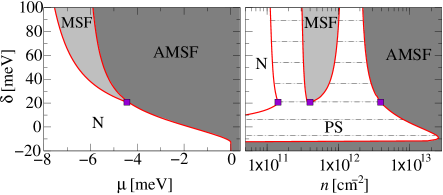
S. Fig. 8: Finite temperature phase diagram for ZnO parameters in the low-momentum quadratic approximation for the LP dispersion, as discussed below, for a temperature $T=11.6$ K. Note that a logarithmic scale has been used for density in the right hand panel.

IV.3 ZnO parameters

For ZnO, while the photon and exciton masses are similar to those of GaAs, $m_{C}=10^{-4}m_{X}$ and $m_{X}=0.2m_{e}$ (for the exciton mass see the Supplementary Information of Ref. Li et al. (2013)), the most important change is the significant increase of biexciton binding energy to $|E_{b}|=18$ meV Makino et al. (2005) (also the exciton binding energy increases from $10$ meV for GaAs to around $85$ meV, depending on the well width). The Rabi-Splitting for ZnO also is typically larger than for GaAs, reaching values up to $200-300$ meV Li et al. (2013). However, for the observation of the MSF phase, it is in fact advantageous to consider a smaller Rabi splitting than the largest values that have been achieved Li et al. (2013); Trichet et al. (2013), and we fix $\Omega_{R}=20$ meV. Reducing the Rabi splitting is easy to achieve, by using a longer microcavity, with a higher mode volume. We hence choose a reasonable value where the MSF phase occurs at easily attainable detunings and temperatures. Supplemental Figure 8 shows a characteristic phase diagram of ZnO at a relatively high temperature of $T=11.6$ K, showing that the MSF phase can in this case be seen for high temperatures and detunings comparable to the Rabi splitting.

References

- Bloch et al. (2008) I. Bloch, J. Dalibard, and W. Zwerger, Rev. Mod. Phys. 80, 885 (2008).
- Chin et al. (2010) C. Chin, R. Grimm, P. Julienne, and E. Tiesinga, Rev. Mod. Phys. 82, 1225 (2010).
- Ketterle and Zwierlein (2008) W. Ketterle and M. W. Zwierlein, Nuovo Cimento Rivista Serie 31, 247 (2008).
- Leggett and Zhang (2012) A. J. Leggett and S. Zhang, in Lecture Notes in Physics, Vol. 836, Lecture Notes in Physics, Vol. 836, edited by W. Zwerger (Springer Berlin Heidelberg, Berlin, Heidelberg, 2012) pp. 33–47.
- Timmermans et al. (1999) E. Timmermans, P. Tommasini, M. Hussein, and A. Kerman, Phys. Rep. 315, 199 (1999).
- Mueller and Baym (2000) E. J. Mueller and G. Baym, Phys. Rev. A 62, 053605 (2000).
- Jeon et al. (2002) G. Jeon, L. Yin, S. Rhee, and D. Thouless, Phys. Rev. A 66, 011603 (2002).
- Kuklov et al. (2004a) A. Kuklov, N. Prokof’ev, and B. Svistunov, Phys. Rev. Lett. 92, 030403 (2004a).
- Kuklov et al. (2004b) A. Kuklov, N. Prokof’ev, and B. Svistunov, Phys. Rev. Lett. 92, 050402 (2004b).
- Radzihovsky et al. (2004) L. Radzihovsky, J. Park, and P. Weichman, Phys. Rev. Lett. 92, 1 (2004).
- Romans et al. (2004) M. Romans, R. Duine, S. Sachdev, and H. Stoof, Phys. Rev. Lett. 93, 020405 (2004).
- Radzihovsky et al. (2008) L. Radzihovsky, P. B. Weichman, and J. I. Park, Ann. Phys. 323, 2376 (2008).
- Basu and Mueller (2008) S. Basu and E. J. Mueller, Phys. Rev. A 78, 53603 (2008).
- Zhou et al. (2008) L. Zhou, J. Qian, H. Pu, W. Zhang, and H. Ling, Phys. Rev. A 78, 053612 (2008).
- Koetsier et al. (2009) A. Koetsier, P. Massignan, R. Duine, and H. Stoof, Phys. Rev. A 79, 063609 (2009).
- Bhaseen et al. (2009) M. J. Bhaseen, M. Hohenadler, A. O. Silver, and B. D. Simons, Phys. Rev. Lett. 102, 135301 (2009).
- Radzihovsky and Choi (2009) L. Radzihovsky and S. Choi, Phys. Rev. Lett. 103, 95302 (2009).
- Hohenadler et al. (2010) M. Hohenadler, A. O. Silver, M. J. Bhaseen, and B. D. Simons, Phys. Rev. A. 82, 1 (2010).
- Ejima et al. (2011) S. Ejima, M. J. Bhaseen, M. Hohenadler, F. H. L. Essler, H. Fehske, and B. D. Simons, Phys. Rev. Lett. 106, 15303 (2011).
- Bhaseen et al. (2012) M. J. Bhaseen, S. Ejima, F. H. L. Essler, H. Fehske, M. Hohenadler, and B. D. Simons, Phys. Rev. A 85, 033636 (2012).
- Zhou and Mashayekhi (2013) F. Zhou and M. S. Mashayekhi, Ann. Phys. 328, 83 (2013).
- Rem et al. (2013) B. S. Rem, A. T. Grier, I. Ferrier-Barbut, U. Eismann, T. Langen, N. Navon, L. Khaykovich, F. Werner, D. S. Petrov, F. Chevy, and C. Salomon, Phys. Rev. Lett. 110, 163202 (2013).
- Kavokin et al. (2007) A. V. Kavokin, J. J. Baumberg, G. Malpuech, and F. P. Laussy, Microcavities (Oxford University Press, Oxford, 2007).
- Carusotto and Ciuti (2013) I. Carusotto and C. Ciuti, Rev. Mod. Phys. 85, 299 (2013).
- Kasprzak et al. (2006) J. Kasprzak, M. Richard, S. Kundermann, A. Baas, P. Jeambrun, J. M. J. Keeling, F. M. Marchetti, M. H. Szymańska, R. André, J. L. Staehli, V. Savona, P. B. Littlewood, B. Deveaud, and L. S. Dang, Nature 443, 409 (2006).
- Balili et al. (2007) R. Balili, V. Hartwell, D. Snoke, L. Pfeiffer, and K. West, Science 316, 1007 (2007).
- Wouters (2007) M. Wouters, Phys. Rev. B 76, 045319 (2007).
- Carusotto et al. (2010) I. Carusotto, T. Volz, and A. Imamoğlu, Europhys. Lett. 90, 37001 (2010).
- Saba et al. (2000) M. Saba, F. Quochi, C. Ciuti, U. Oesterle, J. Staehli, B. Deveaud, G. Bongiovanni, and A. Mura, Phys. Rev. Lett. 85, 385 (2000).
- Borri et al. (2003) P. Borri, W. Langbein, and U. Woggon, Semicond. Sci. Technol. 18, S351 (2003).
- Wen et al. (2013a) P. Wen, G. Christmann, J. J. Baumberg, and K. A. Nelson, New J. Phys. 15, 025005 (2013a).
- Takemura et al. (2014) N. Takemura, S. Trebaol, M. Wouters, M. T. Portella-Oberli, and B. Deveaud, Nat Phys 10, 500 (2014).
- Takemura et al. (2013) N. Takemura, S. Trebaol, M. Wouters, M. T. Portella-Oberli, and B. Deveaud, (2013), arXiv:1310.6506 .
- Wen et al. (2013b) P. Wen, Y. Sun, K. A. Nelson, B. Nelsen, G. Liu, M. Steger, D. W. Snoke, L. N. Pfeiffer, and K. West, “Phase diagram of Bose condensation of long-lifetime polaritons in equilibrium,” (2013b).
- (35) See Supplemental Material at … for derivation of effective model, details of pair coherence detection scheme, and further cuts throughg phase diagram.
- Gurarie and Radzihovsky (2007) V. Gurarie and L. Radzihovsky, Ann. Phys. 322, 2 (2007).
- Wouters and Carusotto (2007) M. Wouters and I. Carusotto, Phys. Rev. B 75, 075332 (2007).
- Mysryowicz (1995) A. Mysryowicz, in Bose-Einstein Condensation, edited by A. Griffin, D. W. Snoke, and S. Stringari (Cambridge University Press, Cambridge, 1995) p. 330.
- Note (1) For imbalanced populations in presence of a Zeeman field, two additional phases are allowed Zhou et al. (2008): , , and , , .
- Nozières and Saint James (1982) P. Nozières and D. Saint James, J. Physique 43, 1133 (1982).
- Kleinert (1995) H. Kleinert, Path Integrals in Quantum Mechanics, Statistics and Polymer Physics (World Scientific, Singapore, 1995).
- Feynman (1998) R. P. Feynman, Statistical Mechanics: A Set Of Lectures (Advanced Books Classics) (Westview Press, 1998) p. 368.
- Pitaevskii and Stringari (2003) L. P. Pitaevskii and S. Stringari, Bose-Einstein Condensation (Clarendon Press, Oxford, 2003).
- Kagan et al. (2000) Y. Kagan, V. A. Kashurnikov, A. V. Krasavin, N. V. Prokof’ev, and B. V. Svistunov, Phys. Rev. A 61, 43608 (2000).
- Prokof’ev and Svistunov (2002) N. Prokof’ev and B. Svistunov, Phys. Rev. A 66, 043608 (2002).
- Popov (1983) V. N. Popov, Functional Integrals in Quantum Field Theory and Statistical Physics (D. Reidel, Dordrecht, 1983).
- Nozieres and Schmitt-Rink (1985) P. Nozieres and S. Schmitt-Rink, J. Low. Temp. Phys. 59, 195 (1985).
- Li et al. (2013) F. Li, L. Orosz, O. Kamoun, S. Bouchoule, C. Brimont, P. Disseix, T. Guillet, X. Lafosse, M. Leroux, J. Leymarie, M. Mexis, M. Mihailovic, G. Patriarche, F. Réveret, D. Solnyshkov, J. Zuniga-Perez, and G. Malpuech, Phys. Rev. Lett. 110, 196406 (2013).
- Trichet et al. (2013) A. Trichet, E. Durupt, F. Médard, S. Datta, A. Minguzzi, and M. Richard, Phys. Rev. B 88, 121407 (2013).
- van Kesteren et al. (1990) H. van Kesteren, E. Cosman, W. van der Poel, and C. Foxon, Phys. Rev. B 41, 5283 (1990).
- Combescot et al. (2007) M. Combescot, O. Betbeder-Matibet, and R. Combescot, Phys. Rev. Lett. 99, 176403 (2007).
- Makino et al. (2005) T. Makino, Y. Segawa, M. Kawasaki, and H. Koinuma, Semicond. Sci. Technol. 20, S78 (2005).