New Approach to Cosmological Fluctuation using the Background Field Method and CMB Power Spectrum

Abstract

A new field theory formulation is presented for the analysis of the CMB power spectrum distribution in the cosmology. The background-field formalism is fully used. Stimulated by the recent idea of the emergent gravity, the gravitational (metric) field $g_{\mu\nu}$ is not taken as the quantum-field, but as the background field. The statistical fluctuation effect of the metric field is taken into account by the path (hyper-surface)-integral over the space-time. Using a simple scalar model on the curved (dS₄) space-time, we explain the above things with the following additional points:  1) Clear separate treatment of the classical effect, the statistical effect and the quantum effect;  2) The cosmological fluctuation comes not from the ’quantum’ gravity but from the unkown ’microscopic’ movement;  3) IR parameter ($\ell$) is introduced for the time axis as the periodicity. Time reversal(Z₂)-symmetry is introduced in order to treat the problem separately with respect to the Z₂ parity. This procedure much helps both UV and IR regularization to work well.

1 Introduction

The more the data of the CMB experiment accumulates, the richer structure of our universe is exposed. In this fascinating period, the CMB spectrum data plays so important role to understand our universe. We approach this spectrum using the background-field method[1] which keeps the important position in the quantum field theory.

The wonderful development of the string theory and D-brane theory has brought us the intimate relation between gravity and (condensed-)matter physics through AdS/CFT correspondence. Especially the relation to the hydrodynamics gradually becomes important through the discussion about the ratio of viscosity and entropy. As the continuum field theory, the gravitational theory and the fluid theory share common problems such as the velocity distribution in the galaxy and that in the rotated (viscous) fluid. Another important recent trend is about the view to the gravitational (metric) field. The standpoint ”emergent gravity”[2] is gradually taken seriously. It claims gravity is not fundamental one, but emerges from the statistical property, such as entropy, of the medium (entropic force).

With these new trends of the gravitational theory, we newly formulate the power spectrum calculation. The spectrum tells us how the light coming from one direction correlates with the other one that comes from another direction. Generally the correlation between the lights from $n$ directions is described by certain n-point function. It corresponds to S-matrix in the quantum field theory. We formulate the $n$-point function using the background-field formalism[1].

2 CMB power spectrum in the background-field formalism

Let us consider the coupled system of the scalar field $\Phi(x)$ and the gravitational (metric) field $g_{\mu\nu}(x)$ in the 3(space)+1(time) dimensional manifold.   $\ \bm{<<}\ S[\Phi;g_{\mu\nu}]={\int d^{4}x}\sqrt{-g}({-1}/{16\pi G_{N}}\cdot\\ (R-2\lambda)+{\cal L}_{mat}),{\cal L}_{mat}\equiv-1/2\cdot{\rm NewA}_{\mu}\Phi{\rm NewA}^{\mu}\Phi-{m^{2}}/{2}\cdot\Phi^{2}-V(\Phi),\ V(\Phi)={\sigma}/{4!}\cdot\Phi^{4},\ (1)\bm{>>}\$   where $\sigma>0$, $G_{N}$ is the Newton’s gravitational constant, $m$ is the scalar mass, and $\lambda$ is the cosmological constant. $V(\Phi)$ is the scalar potential. ${\cal L}_{mat}$ is the matter($\Phi$) part of the Lagrangian. The used notaion is $(x^{\mu})=(x^{0},x^{1},x^{2},x^{3})\equiv(t,x,y,z),\ -\infty<t,x,y,z<+\infty$. We expand the scalar-field around its classical background field ($\Phi_{cl}$) in order to quantize the matter-field in the background-field formalism: $\Phi=\Phi_{cl}+\varphi$, where $\Phi_{cl}$ is the classsical solution of the matter part ((B) of (3)). The effective action $\Gamma[\Phi_{cl};g_{\mu\nu}]$ is defined as   $\ \bm{<<}\ {\rm e}^{i\Gamma[\Phi_{cl};g_{\mu\nu}]}=\int{\cal D}\varphi\exp i\left\{S[\Phi_{cl}+\varphi;g_{\mu\nu}]-{\delta S[\Phi_{cl};g_{\mu\nu}]}/{\delta\Phi_{cl}}\cdot\varphi\right\}.\ (2)\bm{>>}\$   Here we do not Taylor-expand the gravitational field, which means, in the present treatment, the gravitational field $g_{\mu\nu}(x)$ is not field-quantized and is treated as the background (classical) field. $\varphi$ is the quantum field. The scalar (matter) field only is quantized.

$\Phi_{cl}$ and $g_{\mu\nu}$ must satisfy the on-shell condition:   $\ \bm{<<}\ \mbox{On-shell Condition}:\ \mbox{(A)}\ \ {\delta\Gamma[\Phi_{cl};g_{\mu\nu}]}/{\delta\Phi_{cl}}=0;\ \mbox{(B)}\ \ {\delta\Gamma[\Phi_{cl};g_{\mu\nu}]}/{\delta g_{\mu\nu}}=0.\ (3)\bm{>>}\$   In the present work, $\Phi_{cl}$ and $g_{\mu\nu}$ are the background fields. At the tree level (of the scalar quantum-loop expansion), Eq.(A) is   $\ \bm{<<}\ {\delta S[\Phi_{cl};g_{\mu\nu}]}/{\delta\Phi_{cl}}=0;\sqrt{-g}\{{\rm NewA}^{2}\Phi_{cl}-m^{2}\Phi_{cl}\}=\sqrt{-g}{\delta V(\Phi_{cl})}/{\delta\Phi_{cl}}.\ (4)\bm{>>}\$   The above solution $\Phi_{cl}$ is formally obtained as   $\ \bm{<<}\ \Phi_{cl}(x)=\Phi_{0}(x)+\int D(x-x^{\prime})\sqrt{-g}({\delta V(\Phi_{cl})}/{\delta\Phi_{cl}})|_{x^{\prime}}d^{4}x^{\prime},\ \sqrt{-g}({\rm NewA}^{2}-m^{2})D(x-x^{\prime})=\delta^{4}(x-x^{\prime}),\ (5)\bm{>>}\$   where $\Phi_{0}$ is the free field, $\sqrt{-g}({\rm NewA}^{2}-m^{2})\Phi_{0}=0$, and $D(x-x^{\prime})$ is the propagator on the curved geometry $g_{\mu\nu}$. ( $\Phi_{0}$ is later used as the external source to generate the n-point function of the spectrum. ) The above equation gives the tree graph expansion where the expansion parameter is a small coupling ($\sigma$ in (1)) in $V(\Phi_{cl})$. (c.f. Loop-expansion (2) is that of the power of $\hbar$. )

On the other hand, Eq.(B) of (3) is, at the tree level, written as   $\ \bm{<<}\ {\delta S[\Phi_{cl};g_{\mu\nu}]}/{\delta g_{\mu\nu}}=0;\ R_{\mu\nu}-1/2\cdot Rg_{\mu\nu}+\lambda g_{\mu\nu}=8\pi G_{N}T_{\mu\nu},\ T^{\mu\nu}={2}/{\sqrt{-g}}\cdot{\delta(\sqrt{-g}{\cal L}_{mat})}/{\delta g_{\mu\nu}},\ T_{\mu\nu}=\partial_{\mu}\Phi_{cl}\partial_{\nu}\Phi_{cl}-g_{\mu\nu}\left(1/2\cdot\partial^{\sigma}\Phi_{cl}\partial_{\sigma}\Phi_{cl}+{m^{2}}/{2}\cdot\Phi_{cl}^{2}+V(\Phi_{cl})\right).\ (6)\bm{>>}\$

3 dS₄ Geometry, Bunch-Davies Vacuum and Casimir Energy

3.1 dS₄ Geometry and Conformal Time

The metric $g_{\mu\nu}$ must satisfy the on-shell condition (3), or (4) and (6) at the tree level. Now we restrict the form of $g_{\mu\nu}$ from the requirement of the space-time symmetry: homogenity and isotropy. $\ \bm{<<}\ ds^{2}=g_{\mu\nu}(x)dx^{\mu}dx^{\nu}=-dt^{2}+a(t)^{2}(dx^{2}+dy^{2}+dz^{2}),\ a(t)={\rm e}^{\rho(t)},\ (7)\bm{>>}\$   where we take the spacially flat case. If we take $a(t)$ as follows :   $\ \bm{<<}\ {\rho(t)}/{t}=H_{0}(\mbox{constant})>0{\quad,}\quad{\rm e}^{H_{0}t}\equiv a_{infl}(t){\quad,}\quad\left(g^{infl}_{\mu\nu}\right)=\mbox{diag}(-1,{\rm e}^{2H_{0}t},{\rm e}^{2H_{0}t},{\rm e}^{2H_{0}t}){\quad,}\quad ds^{2}=g_{\mu\nu}^{infl}(x)dx^{\mu}dx^{\nu}=-dt^{2}+{\rm e}^{2H_{0}t}(dx^{2}+dy^{2}+dz^{2}){\quad,}\quad-\infty<t,x,y,z<\infty{\quad,}\ (8)\bm{>>}\$   the space-time geometry becomes 4dim de Sitter (dS₄) which describes the inflation universe. $H_{0}$ is a positive constant (Hubble constant).

In the following of this section, we consider the dS₄ metric, $g_{\mu\nu}^{infl}$, as the background field. We now transform from $t$ to the conformal time $\eta$ defined by   $\ \bm{<<}\ d\eta={\rm e}^{-H_{0}t}dt{\quad,}\quad\eta=-{1}/{H_{0}}\cdot{\rm e}^{-H_{0}t}{\quad,}\quad-\infty<t<\infty{\quad,}\quad-\infty<\eta<0.\ (9)\bm{>>}\$   The metric transforms to the conformally-flat type.   $\ \bm{<<}\ ds^{2}=g_{\mu\nu}^{infl}(x)dx^{\mu}dx^{\nu}={\tilde{g}}_{\mu\nu}(\chi)d\chi^{\mu}d\chi^{\nu}={1}/{(H_{0}\eta)^{2}}\cdot(-d\eta^{2}+dx^{2}+dy^{2}+dz^{2}),\ \sqrt{-{\tilde{g}}}={1}/{(H_{0}\eta)^{4}},\ (\chi^{\mu})=(\chi^{0},\chi^{1},\chi^{2},\chi^{3})=(\eta,x,y,z),\ (10)\bm{>>}\$   The perturbative solution $\Phi_{cl}$, (5), is given by   $\ \bm{<<}\ \Phi_{cl}(\chi)=\Phi_{0}(\chi)+\int{\tilde{D}}(\chi,\chi^{\prime})~{}\left.\frac{1}{(H_{0}\eta^{\prime})^{4}}\frac{\delta V(\Phi_{cl})}{\delta\Phi_{cl}}\right|_{\chi^{\prime}}d^{4}\chi^{\prime},\ \sqrt{-{\tilde{g}}}({\tilde{\nabla}}^{2}-m^{2})\Phi_{0}=-\left\{\partial_{\eta}\frac{1}{(H_{0}\eta)^{2}}\partial_{\eta}+\frac{m^{2}}{(H_{0}\eta)^{4}}-\frac{1}{(H_{0}\eta)^{2}}{\vec{\nabla}}^{2}\right\}\Phi_{0}=0,\ (11)\bm{>>}\$   where ${\tilde{\nabla}}^{2}={\tilde{g}}^{\mu\nu}{\tilde{\nabla}}_{\mu}{\tilde{\nabla}}_{\nu}\ ({\tilde{\nabla}}_{\mu}=\partial/\partial\chi^{\mu}+\cdots)$ and $\Phi_{0}$ is the free field. ${\tilde{D}}(\chi,\chi^{\prime})$ is the propagator on the dS₄ geometry ${\tilde{g}}_{\mu\nu}(\chi)$ ( or $g^{infl}_{\mu\nu}(x)$).   $\ \bm{<<}\ \sqrt{-{\tilde{g}}}({\tilde{\nabla}}^{2}-m^{2}){\tilde{D}}(\chi,\chi^{\prime})=\\ -\left\{\partial_{\eta}\frac{1}{(H_{0}\eta)^{2}}\partial_{\eta}+\frac{m^{2}}{(H_{0}\eta)^{4}}-\frac{1}{(H_{0}\eta)^{2}}{\vec{\nabla}}^{2}\right\}{\tilde{D}}(\chi,\chi^{\prime})=\delta^{4}(\chi-\chi^{\prime}),\ (12)\bm{>>}\$

3.2 Z₂ Symmetry, Periodicity and IR parameter $\ell$

In the (matter-field) quantization on dS_n (and AdS_n) geometry, the control of the IR-divergence is important[3]. In order to regularize the IR behavior, we introduce the following symmetries in the time coordinate $t$:   $\ \bm{<<}\ \mbox{Z}_{2}\mbox{ Symmetry}:\ \ t\ \leftrightarrow\ -t,\ \ \mbox{Periodicity}:\ \ t\rightarrow t+2\ell,\ (12b)\bm{>>}\$   where $\ell$ is the period parameter (IR parameter). As for the conformal time, we redefine it as follows,   $\ \bm{<<}\ \eta=\left\{\begin{array}[]{cccc}-{1}/{H_{0}}\cdot{\rm e}^{-H_{0}t}\ ,&d\eta=-H_{0}\eta dt\ ,&0<t<\ell\ ,&{-1}/{H_{0}}\cdot<\eta<{-1}/{\omega}\\ +{1}/{H_{0}}\cdot{\rm e}^{H_{0}t}\ ,&d\eta=H_{0}\eta dt\ ,&-\ell<t<0\ ,&{1}/{\omega}<\eta<{1}/{H_{0}}\end{array}\right.\ (13)\bm{>>}\$   ($\omega\equiv{\rm e}^{\ell H_{0}}H_{0}\gg\ H_{0}$) which leads to the relation $\eta\leftrightarrow-\eta$ corresponding to the Z₂ symmetry in (12b). In this definition the far past ($t\rightarrow-\ell$) corresponds to $\eta\rightarrow 1/\omega$, the far future ($t\rightarrow+\ell$) corresponds to $\eta\rightarrow-1/\omega$. $t=\mp 0$ correspond to the singular points $\eta=\pm 1/H_{0}$. See Fig.1.

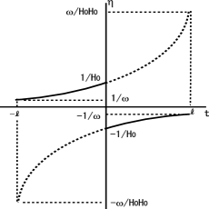
Figure 1: Conformal time ($\eta$) versus ordinary time ($t$). Time-reversal correspondence is valid. Eq.(13)

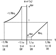
Figure 2: Scale factor in dS₄ geometry. Eq.(14).

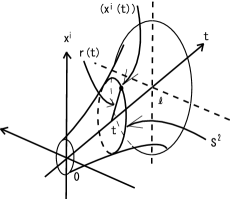
Figure 3: Hyper-surface in dS₄ space-time. Eq.(23b).

Hence $a_{inf}(t)={\rm e}^{H_{0}t}$ is expressed as
$\ \bm{<<}\ 0<t<\ell\ (-{1}/{H_{0}}<\eta<{-1}/{\omega})\ :\quad\eta=-{{\rm e}^{-H_{0}t}}/{H_{0}}{\quad,}\quad d\eta=-H_{0}\eta dt{\quad,}\quad a_{inf}(\eta)=-{1}/{H_{0}\eta}\\ -\ell<t<0\ ({1}/{\omega}<\eta<{1}/{H_{0}})\ :\quad\eta={{\rm e}^{H_{0}t}}/{H_{0}}{\quad,}\quad d\eta=H_{0}\eta dt{\quad,}\quad a_{inf}(\eta)=H_{0}\eta\ (14)\bm{>>}\$   See Fig.2.

Let us switch, from $\Phi_{0}(\eta,{\vec{x}})$ and ${\tilde{D}}(\chi,\chi^{\prime})$, to the spacially-Fourier-transformed expression $\phi_{{\vec{p}}}(\eta)$ and ${\tilde{D}}_{\vec{p}}(\eta,\eta^{\prime})$:   $\ \bm{<<}\ \Phi_{0}(\eta,{\vec{x}})=\int{d^{3}{\vec{p}}}/{(2\pi)^{3}}\cdot{\rm e}^{i{\vec{p}}\cdot{\vec{x}}}\phi_{{\vec{p}}}(\eta),\ {\tilde{D}}(\chi,\chi^{\prime})=\int{d^{3}{\vec{p}}}/{(2\pi)^{3}}\cdot{\rm e}^{i{\vec{p}}\cdot({\vec{x}}-{\vec{x}}^{\prime})}{\tilde{D}}_{\vec{p}}(\eta,\eta^{\prime}),\ (15)\bm{>>}\$   where ${\tilde{D}}_{\vec{p}}(\eta,\eta^{\prime})$ is called ’Momentum/Position propagator’[3]. From (11), $\phi_{{\vec{p}}}(\eta)$ satisfies the following Bessel eigenvalue equation.   $\ \bm{<<}\ \left\{{\partial_{\eta}}^{2}-{2}/{\eta}\cdot\partial_{\eta}+{m^{2}}/{(H_{0}\eta)^{2}}+M^{2}\right\}\phi_{M}(\eta)=\{s(\eta)^{-1}{\hat{L}}_{\eta}+M^{2}\}\phi_{M}(\eta)=0,\ M^{2}\equiv{\vec{p}}^{2},\ s(\eta)\equiv{1}/{(H_{0}\eta)^{2}},\ (16)\bm{>>}\$   where ${\hat{L}}_{\eta}\equiv\partial_{\eta}s(\eta)\partial_{\eta}+{m^{2}}/{(H_{0}\eta)^{4}}$. From (12), ${\tilde{D}}_{\vec{p}}(\eta,\eta^{\prime})$ satisfies
$\ \bm{<<}\ \{{\hat{L}}_{\eta}+{\vec{p}}^{2}s(\eta)\}{\tilde{D}}_{{\vec{p}}}^{\mp}(\eta,\eta^{\prime})=\left\{\begin{array}[]{cc}\epsilon(\eta)\epsilon(\eta^{\prime}){\hat{\delta}}(|\eta|-|\eta^{\prime}|)&\mbox{for P=}-\\ {\hat{\delta}}(|\eta|-|\eta^{\prime}|)&\mbox{for P=}+\end{array}\right.\ (17)\bm{>>}\$   where $\epsilon(\eta)$ is the sign function.

The Bessel equation (16) gives us the free field wave function as  $\phi_{M}(\eta)=\eta^{3/2}Z_{\nu}(M\eta){\quad,}\quad\nu=\sqrt{(3/2)^{2}-(m/H_{0})^{2}}$, where $\nu=0,1/2,\sqrt{5}/2,$ and $3/2$ correspond to $m=(3/2)H_{0},\sqrt{2}H_{0},H_{0},$ and $0$ respectively. When $m$ is non-negative real number, the scalar mass has the upper-bound: $0\leq m\leq(3/2)H_{0}$. (We may also consider the imaginary mass: $m^{2}<0$. )

3.3 Boundary Condition, Bunch-Davies Vacuum and Casimir Energy

As for the boundary condition for Z₂-parity odd free field ($P=-$), we take the following one based on the requirement of the continuity at $\eta=\pm 1/\omega,\pm 1/H_{0}$ ($t=\mp\ell,\mp 0$): $\Phi_{0}(\eta\rightarrow\pm 1/\omega,{\vec{x}})=0(\mbox{Dirichlet}),\ \Phi_{0}(\eta\rightarrow\pm 1/H_{0},{\vec{x}})=0(\mbox{Dirichlet})$. As for the boundary condition for Z₂-parity even case ($P=+$), we take the following one based on the requirement of the smoothness at $\eta=\pm 1/\omega,\pm 1/H_{0}$ ($t=\mp\ell,\mp 0$): $\left.\partial_{\eta}\Phi_{0}\right|_{\eta\rightarrow\pm 1/\omega}=0(\mbox{Neumann}),\ \left.\partial_{\eta}\Phi_{0}\right|_{\eta\rightarrow\pm 1/H_{0}}=0(\mbox{Neumann})$.

Casimir energy is given by $\sigma$-independent part (free part) of the 1-loop effective action in (2). $\ \bm{<<}\ \exp[i\Gamma^{\mbox{1-loop}}]=\exp\left[\int{d^{3}{\vec{p}}}/{(2\pi)^{3}}\cdot 2\int_{-1/H_{0}}^{-1/\omega}d\eta\{-1/2\cdot\ln(-s(\eta)^{-1}{\hat{L}}_{\eta}-{\vec{p}}^{2})\}\right]=\exp\int_{0}^{\infty}{d\tau}/{\tau}\cdot 1/2\cdot\Tr H_{\vec{p}}(\eta,\eta^{\prime};\tau),\ (18)\bm{>>}\$   where $H_{\vec{p}}(\eta,\eta^{\prime};\tau)$ is the Heat-Kernel:   $\ \bm{<<}\{{\partial}/{\partial\tau}-(s^{-1}{\hat{L}}_{\eta}+{\vec{p}}^{2})\}H_{\vec{p}}(\eta,\eta^{\prime};\tau)=0,\ H_{\vec{p}}(\eta,\eta^{\prime};\tau)=(\eta|{\rm e}^{(s^{-1}{\hat{L}}_{\eta}+{\vec{p}}^{2})\tau}|\eta^{\prime}).\ (19)\bm{>>}$   This is a formal expression using Dirac’s abstract states $|\eta),(\eta|$. It is rigorously defined by using the complete and orthogonal eigen functions { $\phi_{n}(\eta)$} of the operator $s^{-1}{\hat{L}}_{\eta}$.
$\ \bm{<<}\ \phi_{n}(\eta)\equiv(n|\eta)=(\eta|n),\ \{s(\eta)^{-1}{\hat{L}}_{\eta}+{M_{n}}^{2}\}\phi_{n}(\eta)=0,\ (\eta|\eta^{\prime})=\left\{\begin{array}[]{lc}(H_{0}\eta)^{2}\epsilon(\eta)\epsilon(\eta^{\prime}){\hat{\delta}}(|\eta|-|\eta^{\prime}|)&\mbox{for }P=-\\ (H_{0}\eta)^{2}\delta(|\eta|-|\eta^{\prime}|)&\mbox{for }P=+\\ \end{array}\right.\\ \left(\int_{-1/H_{0}}^{-1/\omega}+\int_{1/\omega}^{1/H_{0}}\right)\frac{d\eta}{(H_{0}\eta)^{2}}(n|\eta)(\eta|k)=2\int_{-1/H_{0}}^{-1/\omega}\frac{d\eta}{(H_{0}\eta)^{2}}(n|\eta)(\eta|k)=(n|k)=\delta_{n,k}{\quad,}\\ \left(\int_{-1/H_{0}}^{-1/\omega}+\int_{1/\omega}^{1/H_{0}}\right)\frac{d\eta}{(H_{0}\eta)^{2}}|\eta)(\eta|=2\int_{-1/H_{0}}^{-1/\omega}\frac{d\eta}{(H_{0}\eta)^{2}}|\eta)(\eta|=1{\quad,}\quad\sum|n)(n|=1.\ (20)\bm{>>}\$
The set { $\phi_{n}(\eta)$} constitutes Bunch-Davies vacuum.

3.4 Wick Rotation for ${\vec{p}}$

From the previous result, we evaluate Casimir energy of the dS₄ space-time.   $\ \bm{<<}\ -H_{0}^{-3}E_{Cas}^{dS4}=\int{d^{3}{\vec{p}}}/{(2\pi)^{3}}\cdot 2\int_{-1/H_{0}}^{-1/\omega}d\eta\{1/2\cdot\int^{\infty}_{0}{d\tau}/{\tau}\cdot(\eta|{\rm e}^{\tau(s(\eta)^{-1}{\hat{L}}_{\eta}+{\vec{p}}^{2})}|\eta)\}=\int_{0}^{\infty}{d\tau}/{\tau}\cdot 1/2\cdot\Tr H_{\vec{p}}(\eta,\eta^{\prime};\tau).\ (21)\bm{>>}\$   This expresssion diverges very badly (UV-divergence). To regularize it, we do
$\ \bm{<<}\ \mbox{Wick rotation for {\it space}-components of momentum}\quad p_{x}\ ,\ p_{y}\ ,\ p_{z}\ \longrightarrow ip_{x}\ ,\ ip_{y}\ ,\ ip_{z}\ (22)\bm{>>}\$ The regularized expression is the same as Casimir energy for (E)AdS₄. The regularized one behaves milder but still diverges.

4 Metric Fluctuation and Averaging Over the 4D Space-Time using the Generalized Path-Integral

We note again the metric field $g_{\mu\nu}(x)$ is treated as the background one. It is defined by the variation equation of $\Gamma[\Phi_{cl};g_{\mu\nu}]$, (B) of (3). Let us express the effective action as the integral of the space-time coordinates $x^{\mu}$: $S=\Gamma[\Phi_{cl}(x);g_{\mu\nu}(x)]\equiv\int d^{4}x{\cal L}[x^{\mu}]$. We regard this quantity as an action for a statistic-mechanical system composed of its dynamical variables ($x^{i}$: $i=1,2,3$) and time ($x^{0}=t$). Here we consider the small fluctuation of coordinates $x^{i}$, keeping $x^{0}=t$ fixed, in the dS₄ geometry $g^{inf}_{\mu\nu}(x)$: $x^{i}\rightarrow x^{i}+\sqrt{\epsilon}f^{i}({\vec{x}},t)={x^{i}}^{\prime},\ t=t^{\prime}\ (x^{0}={x^{0}}^{\prime})$, where $\epsilon$ is a small positive parameter for dictating the perturbation order. ( We regard the present system not as the (metric) field theory but as the statistic-mechanical system of space coordinates ${\bf x}$ and time $t$. Hence this fluctuation should not be regarded as the gauge variation. ) This fluctuation can be absorbed into the metric fluctuation (around $g^{inf}_{\mu\nu}$) as the requirement of the invariance of the line element (general coordinate invariance).
$\ \bm{<<}\ g^{inf}_{\mu\nu}(x)d{x^{\mu}}^{\prime}d{x^{\nu}}^{\prime}={g_{\mu\nu}}^{\prime}(x)dx^{\mu}dx^{\nu}{\quad,}\quad{g_{\mu\nu}}^{\prime}(x)=g_{\mu\nu}^{inf}(x)+\epsilon h_{\mu\nu}(x),\ h_{00}={\rm e}^{2H_{0}t}\partial_{0}f^{i}\cdot\partial_{0}f^{i}{\quad,}\\ h_{0i}=h_{i0}={\rm e}^{2H_{0}t}\partial_{i}f^{j}\cdot\partial_{0}f^{j},\ h_{ij}={\rm e}^{2H_{0}t}\partial_{i}f^{k}\cdot\partial_{j}f^{k},\ \{{\frac{1}{2}}(\partial_{i}f^{j}+\partial_{j}f^{i})dx^{j}+2\partial_{0}f^{i}dt\}dx^{i}=0.\ (23)\bm{>>}\$ We see the coordinates-fluctuation produces the metric- fluctuation (around the homogeneous and isotropic (dS₄) metric) , as far as the above constraint is preserved. The constraint comes from the difference in the perturbation order between the metric fluctuation ($\epsilon$) and the coordinate fluctuation ($\sqrt{\epsilon}$).

A cause of the fluctuation is the effect of the underlying unknown ’micro’ dynamics (just like Brownian motion of nano-particles in liquid and gas in the early days of the atomic physics). We treat it as the statistical fluctuation phenomena. We adopt the following strategy to compute the fluctuation effect. The coordinates are fluctuating ( , and the metric is also fluctuating as stated in the previous paragraph, ) in a statistical ensemble. In order to compute the statistical average, we must specify the statistical distribution. We note again that this effect is treated, in the present standpoint, not as the quantum one but as purely the statistical one. In order to specify the statistical ensemble in the geometrically-meaningful way, we prepare the following 3 dimensional hyper-surface in dS₄ space-time based on the isotropy requirement in space ($x,y,z$): $\ \bm{<<}\ x^{2}+y^{2}+z^{2}=r(t)^{2},\ (23b)\bm{>>}\$ where $r(t)$ is the radius of S² in the 3D plane standing at t of the time axis. See Fig.4. $r(t)$ is an arbitrary function and will be used for the averaging by considering all possible forms.

The hyper-surface is specified by $r(t)$. In the following path-integral, we regard the hyper-surface as a (generalized) path. On the path (23b), we obtain the induced metric $g_{ij}$ as   $\ \bm{<<}\ ds^{2}=g^{infl}_{\mu\nu}dx^{\mu}dx^{\nu}=-dt^{2}+{\rm e}^{2H_{0}t}dx^{i}dx^{i}=(-\frac{1}{r^{2}\dot{r}^{2}}x^{i}x^{j}+\delta^{ij}{\rm e}^{2H_{0}t})dx^{i}dx^{j}\equiv g_{ij}dx^{i}dx^{j},\ (24)\bm{>>}\$   The constraint in (23) reduces to   $\ \bm{<<}\ \{{\frac{1}{2}}(\partial_{i}f^{j}+\partial_{j}f^{i})v^{j}+2\partial_{0}f^{i}\}v^{i}=0,\ v^{i}\equiv\frac{dx^{i}}{dt},\ f^{i}=f^{i}({\vec{x}}(t),t),\ {\frac{1}{2}}v^{i}{\vec{v}}\cdot\partial_{i}{\vec{f}}+{\frac{1}{2}}\{({\vec{v}}\cdot{\rm NewA}){\vec{f}}\}\cdot{\vec{v}}+\partial_{0}{\vec{f}}\cdot{\vec{v}}=0,\ (25)\bm{>>}\$   In the last formula, Lagrange derivative (which is used in the hydrodynamics) appears. As the geometrical quantity to define the statistical distribution, we take the area $A$ of the hypersurface.   $\ \bm{<<}\ A[x^{i},\dot{x}^{i}]=\int\sqrt{\det g_{ij}}~{}d^{3}{\vec{x}}=\frac{2\sqrt{2}}{3}\int_{0}^{\ell}{\rm e}^{-3H_{0}t}\sqrt{\dot{r}^{2}-{\rm e}^{-2H_{0}t}}~{}dt.\ (26)\bm{>>}\$   Hence the averaged (over the fluctuation) effective action is given by   $\bm{<<}\ \Gamma^{avg}[\Phi_{cl};g_{\mu\nu}]=\int_{1/\Lambda}^{1/\mu}d\rho\int_{r(0)=\rho,r(\ell)=\rho}{\cal D}x^{i}(t)\times\Gamma[\Phi_{cl}({\vec{x}}({\tilde{t}}),{\tilde{t}});g_{\mu\nu}({\vec{x}}({\tilde{t}}),{\tilde{t}})]\exp(-\frac{1}{2\alpha^{\prime}}A[x^{i},\dot{x}^{i}]).\ (26b)\bm{>>}$   where $\mu,\Lambda$ and $\frac{1}{\alpha^{\prime}}$ are IR cutoff, UV cutoff and the surface tension parameter respectively.

More generally, we can consider, instead of $A/2\alpha^{\prime}$,   $\ \bm{<<}\ H[x^{i},\dot{x}^{i}]=\int\sqrt{\det g_{ij}}~{}({1}/{2\alpha^{\prime}}+{1}/{2\kappa}\cdot{\hat{R}}(g_{ij})+O({\partial_{i}}^{4}))d^{3}{\vec{x}},\ \ (27)\bm{>>}\$   where $\kappa$ is the gravitational constant on the 3D hyper-surface. ${\hat{R}}(g_{ij})$ is the curvature of the 3D hyper-surface. We regard $\alpha^{\prime}$ and $\kappa$ as model-parameters to describe the power spectrum.

The 2-point function of the spectrum is given by[1]
$\ \bm{<<}\ \mbox{2-Point Function}\ \ \delta^{2}\Gamma^{avg}/\delta{\tilde{\Phi}}_{0}(t)\delta{\tilde{\Phi}}_{0}(t^{\prime}),\ {\tilde{\Phi}}_{0}(t_{1})\equiv\Phi_{0}({\vec{x}}(t_{1}),t_{1}),\ (28)\bm{>>}\$   See Fig.5.

Natural extension of the above model is AdS₅ extra-dimensional one.
$\ \bm{<<}\ \mbox{2-Point Function}\ \ \delta^{2}\Gamma^{avg}/\delta{\tilde{\Phi}}_{0}(w)\delta{\tilde{\Phi}}_{0}(w^{\prime}),\ {\tilde{\Phi}}_{0}(w_{1})\equiv\Phi_{0}({\vec{x}}(w_{1}),t(w_{1}),w_{1}),t(w)=t(w^{\prime})=i\tau.\ (29)\bm{>>}$   See Fig.5.

5 Discussion and Conclusion

We have presented a new approach to the cosmological fluctuation[4,5,6,7]. It is regarded as the statistical fluctuation of space-coordinates due to the un-known ”micro” dynamics. We adopt the (generalized) path-integral formalism to introduce the statistical ensemble. In the formulation, the geometric object (area $A$, (26)) is taken as the key quantity which determines the statistical distribution. In this new model some new parameters appear: surface tension ($1/\alpha^{\prime}$), IR parameter ($\ell$), IR cut-off ($\mu$), UV cut-off ($\Lambda$), etc.. They are taken to explain the observational data.

References:
[1] L.D. Faddeev and A.A. Slavnov, ”Gauge Fields: Introduction to Quantum Theory”, Benjamin/Cummings Pub., C1980, and references therein;
[2] E. Verlinde, arXiv:1001.0785[hep-th] and references therein;
[3] L. Randall and M. D. Schwartz, JHEP 0111:003, 2001, arXiv:0108114[hep-th]:
[4] S. Ichinose, Jour. Phys. Conf. Ser. 384(2012)012028, arXiv:1205.1316;
[5] S. Ichinose, Jour.Phys.:Conf.Scr.222(2010)012048, arXiv:1001.0222;
[6] S. Ichinose, Prog.Theor.Phys. 121(2009)727, ArXiv:0801.3064v8;
[7] S. Ichinose, ”Geometric Approach to Quant. Stat. Mech. and Minimal Area Principle”, arXiv:1004.2573.

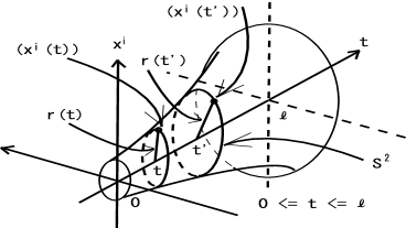
Figure 4: Two points ${\vec{x}}(t),{\vec{x}}(t^{\prime})$ in (28).

Figure 5: Two points ($t(w),{\vec{x}}(w)$), ($t(w^{\prime}),{\vec{x}}(w^{\prime})$) in (29). $t(w)=t(w^{\prime})=i\tau\ ,\ {\vec{x}}\cdot{\vec{x}}+\tau^{2}=r^{2}(w)\ ,\ {\vec{x}}^{\prime}\cdot{\vec{x}}^{\prime}+\tau^{2}=r^{2}(w^{\prime})$ .