SFB/CPP-13-54 TTP13-28
Colour octet potential to three loops

Abstract

We consider the interaction between two static sources in the colour octet configuration and compute the potential to three loops. Special emphasis is put on the treatment of pinch contributions and two methods are applied to reduce their evaluation to diagrams without pinches.

PACS numbers: 12.38.-t, 12.38.Bx

1 Introduction

The potential energy between two heavy quarks is a fundamental quantity in physics. In fact, the history of computing loop corrections to the potential of quarks forming a colour singlet configuration goes back to the mid-seventies with the idea to describe a bound state of heavy coloured objects in analogy to the hydrogen atom [1]. One-loop corrections were computed shortly afterwards in Refs. [2, 3]. The two-loop corrections have only been evaluated towards the end of the nineties by two groups [4, 5, 6] and about five years ago the three-loop corrections have been considered in Refs. [7, 8, 9], again in two independent calculations.

In this paper we consider the potential in momentum space which we define as

$$V^{[c]}(|{\vec{q}}\,|) = -{4\pi C^{[c]}\frac{\alpha_{s}(|{\vec{q}}\,|)}{{\vec{q}}\,^{2}}}\Bigg{[}1+\frac{\alpha_{s}(|{\vec{q}}\,|)}{4\pi}a_{1}^{[c]}+\left(\frac{\alpha_{s}(|{\vec{q}}\,|)}{4\pi}\right)^{2}a_{2}^{[c]}$$ (1)

$$\mbox{}+\left(\frac{\alpha_{s}(|{\vec{q}}\,|)}{4\pi}\right)^{3}\left(a_{3}^{[c]}+8\pi^{2}C_{A}^{3}\ln\frac{\mu^{2}}{{\vec{q}}\,^{2}}\right)+\cdots\Bigg{]}\,,$$

where $C_{A}=N_{c}$ and $C_{F}=(N_{c}^{2}-1)/(2N_{c})$ are the eigenvalues of the quadratic Casimir operators of the adjoint and fundamental representations of the $SU(N_{c})$ colour gauge group, respectively. The strong coupling $\alpha_{s}$ is defined in the $\overline{\rm MS}$ scheme and for the renormalization scale we choose $\mu=|{\vec{q}}\,|$ in order to suppress the corresponding logarithms. The general results, both in momentum and coordinate space, can be found in Appendix A.

In Eq. (1) we have introduced the superscript ${[c]}$ which indicates the colour state of the quark-anti-quark system. In Refs. [4, 5, 6, 7, 8, 9] only the singlet configurations ($c=1$) have been considered, which is phenomenologically most important. However, quarks in the fundamental representation can also combine to a colour octet state. At tree-level and one-loop order only the overall colour factor changes from $C^{[1]}=C_{F}$ to $C^{[8]}=C_{F}-C_{A}/2$. Starting from two loops [10, 11] the coefficients $a_{i}^{[c]}$ get additional contributions. In this paper we compute $a_{3}^{[8]}$ and compare the result to $a_{3}^{[1]}$ [7, 8, 9].

The term proportion to $\ln\mu^{2}$ in Eq. (1) has its origin in an infra-red divergence which has been subtracted minimally. It appears for the first time at three-loop order [12] and is canceled against the ultraviolet divergence of the ultrasoft contributions which have been studied in Refs. [13, 14, 15]. As anticipated in Eq. (1), the ultrasoft contribution for the colour-singlet and colour-octet case differs only by the overall colour factor which is confirmed by our explicit calculation.

Let us for completeness mention that it is possible to generalize the concept of the heavy-quark potential to generic colour sources which in principle can also be in the adjoint representation of $SU(3)$ as, e.g., the gluino in supersymmetric theories. Various combinations of quark, squark and gluino bound state systems have been considered in Ref. [11] and the corresponding potential has been evaluated up to two loops.

A further generalization of the three-loop corrections to $V^{[1]}$ has been considered in Ref. [16] where it is still assumed that the heavy sources form a colour singlet state, however, the colour representation is kept general.

The remainder of the paper is organized as follows: in the next Section we explain in detail how we treat the diagrams involving pinches. Afterwards we present our results in Section 3 and conclude in Section 4.

2 Calculation

As compared to the singlet case the calculation of the octet potential is substantially more complicated which is connected to the occurrence of so-called pinch contributions as shall be discussed in the following. Pinch contributions occur in those cases where a deformation of the integration contour, needed to circumvent poles in the complex plane of the zero-component of the integration momentum, is not possible.

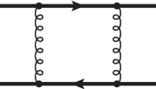
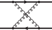
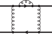
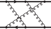
(a)	(b)	(c)	(d)
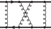
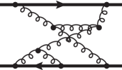
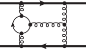
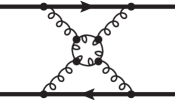
(e)	(f)	(g)	(h)

Figure 1: Feynman diagrams up to three-loop order contributing to $V^{[c]}$. Thick lines represent static quarks, thin solid lines massless fermions and curled lines gluons.

For illustration let us consider the planar ladder diagram in Fig. 1(a). Since the momentum transfer $q$ between the heavy quarks is space-like and the static propagators only contain the energy component of the momentum we obtain for the loop integral the expression

$$\int{\rm d}^{D}k\,f(k,\vec{q}\,)\,\frac{1}{(k_{0}+i0)(k_{0}-i0)}\,,$$ (2)

where $f(\vec{q}\,)$ collects all prefactors and the contribution from the gluon propagators, and $D=4-2\epsilon$ is the space-time dimension.

There are several possibilities to treat the one-loop diagram in Eq. (2) and obtain a relation to a well-defined integral. For example, it is possible to apply the principle value prescription

$$\frac{1}{(k_{0}+i0)(k_{0}-i0)} \to \frac{1}{2}\left[{1\over(k_{0}+i\varepsilon)^{2}}+\frac{1}{(k_{0}-i\varepsilon)^{2}}\right]\,,$$ (3)

which is valid in the soft region for the integration momenta. With the help of Eq. (3) it is possible to treat all contributions involving pinches in one loop momentum [10, 11, 17]. The application to diagrams with two or more pinch contributions in one diagram, a situation which appears at two loops and beyond, is not obvious.

Another possibility is based on the fact that in QED with only one (heavy) lepton pair the potential between the fermion and anti-fermion is given by the tree-level term (see, e.g., discussion in Refs. [18, 7]) which means that the loop corrections are exactly canceled by the iteration terms of lower-order contributions. The latter arise from the fact that the potential is proportional to the logarithm of the quark-anti-quark four-point amplitude which has to be expanded in the coupling constant. Translating this knowledge to QCD means that the sum of all one-loop contributions proportional to $C_{F}^{2}$ have to vanish which in turn leads to the graphical equation

$$\begin{matrix}\includegraphics{figs/example1l}\,.\end{matrix}$$ (4)

In this way the planar-ladder contribution can be replaced by the crossed ladder which is free of pinch contributions. The same method has successfully been applied at two loops [10, 11, 17] [see Ref. [17] for the two-loop analogue of Eq. (4)].

In the following we provide a general prescription for the treatment of the pinch contributions which works to all loop orders and for arbitrary number of involved propagators. We formulate the algorithm in a way which is convenient for our application. Alternative formulations can be found in Refs. [2, 18].

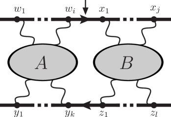
Figure 2: Generic Feynman diagram involving a pinch contribution. The blobs $A$ and $B$ may contain further pinches which are treated recursively (see description of algorithm). The arrow indicates where the static line is cut at first.

It is convenient to formulate the algorithm in coordinate space. Using the Feynman rules from Appendix B the one-loop ladder diagram in Fig. 1(a) takes the form

$$g_{s}^{4}\int\limits_{-\frac{T}{2}}^{\frac{T}{2}}dw_{0}\int\limits_{-\frac{T}{2}}^{\frac{T}{2}}dx_{0}\int\limits_{-\frac{T}{2}}^{\frac{T}{2}}dy_{0}\int\limits_{-\frac{T}{2}}^{\frac{T}{2}}dz_{0}\;\theta\left(x_{0}-w_{0}\right)\theta\left(z_{0}-y_{0}\right)$$

$$\hskip 107.63855pt\times D_{00}\left(w_{0}-y_{0},\vec{r}\right)D_{00}\left(x_{0}-z_{0},\vec{r}\right)\,,$$ (5)

where the colour structure has been ignored. In Eq. (5) the integration over the spacial components has been performed and the $\theta$ functions of the vertices have been used to restrict the integration limits of the temporal integrals to $[-T/2,T/2]$. Note that $\theta(x_{0}-w_{0})$ refers to the upper and $\theta(y_{0}-z_{0})$ to the lower source line. In analogy one obtains for the generic diagram in Fig. 2 the following combination of $\theta$ functions:

$$\theta\left(w^{0}_{2}-w^{0}_{1}\right)\dots\theta\left(w^{0}_{i}-w^{0}_{i-1}\right)\theta\left(x^{0}_{1}-w^{0}_{i}\right)\theta\left(x^{0}_{2}-x^{0}_{1}\right)\dots\theta\left(x^{0}_{j}-x^{0}_{j-1}\right)\,.$$ (6)

A crucial ingredient to the algorithm described below is the cut of a static propagator. This is equivalent to setting the corresponding propagator to unity, i.e., the associated $\theta$ function in Eq. (6) is set to one. Actually, the omission of $\theta(x_{1}-w_{i})$ from Eq. (6) (see also Fig. 2) relaxes the original conditions on the zero components

$$w^{0}_{1}<\dots<w^{0}_{i}<x^{0}_{1}<\dots<x^{0}_{j}\text{.}$$ (7)

to

$$w^{0}_{1}<\dots<w^{0}_{i}\wedge x^{0}_{1}<\dots<x^{0}_{j}\,.$$ (8)

The latter is satisfied by all Feynman diagrams which are obtained from the original one by permutations of vertices in the upper source line as long as the order of the vertices involving $w$’s and $x$’s is kept. Thus the result for the cut diagram is obtained by summing all such contributions. Let us illustrate this mechanism by the following three-loop diagram

$$\begin{matrix}\includegraphics{figs/example_cut}\,.\end{matrix}$$ (9)

The procedure for cutting an anti-source propagator is, of course, in close analogy.

We are now in the position to describe the algorithm which can be applied to all diagrams involving pinch contributions. The output of the algorithm are equations which relate pinch diagrams to diagrams without pinches. The latter can be computed along the lines of Refs. [7, 8, 9]. In all steps QED-like colour factors are assumed; the multiplication with the proper colour factor happens after applying the obtained relations. In parallel to the description of the algorithm we illustrate its principle of operation on explicit two- and three-loop examples.

1. Consider a diagram with a pinch. In case there is more than one pinch the following steps have to be applied to each one consecutively. In case more than one source or anti-source propagator is involved [see, e.g., Fig. 1(c)] the operations are performed for the most left and most right propagator and the resulting equations are added.

2. Express the pinch diagram by the corresponding diagram with a cut source propagator and the remaining contributions according to Eq. (9).

   For our three-loop example the corresponding equation looks as follows

   $$\begin{matrix}\includegraphics{figs/example1}\,.\end{matrix}$$ (10)

3. Replace the diagram with a cut source propagator by the diagram where both the source and anti-source propagators are cut and the remaining contributions which are obtained in analogy to step 1. Write the diagram with two cuts as a product of lower-order contributions.

   The application of these rules to our example leads to

   $$\begin{matrix}\includegraphics{figs/example2}\,.\end{matrix}$$ (11)

4. In a next step the diagrams with a cut in the source propagator have to be treated. This is done by replacing them by the sum of diagrams obtained by considering all allowed permutations of the source vertices.

   In our example this leads to

   $$\begin{matrix}\includegraphics{figs/example3}\,.\end{matrix}$$ (12)

5. Solve the resulting equation for the considered pinch diagram.

   In our example the original diagram appears on the right-hand side with a negative sign. This finally leads to

   $$\begin{matrix}\includegraphics{figs/example4}\,.\end{matrix}$$ (13)

   Note that all diagrams on the right-hand side of this equation are either products of lower-order contributions or are free of pinches and can thus be computed in the standard way.

6. It might be that during the described procedure scaleless integrals appear which are set to zero within dimensional regularization. This is in particular true for non-amputated diagrams.

7. It is advantageous to add diagrams with the same colour factor before applying the described algorithm since in some cases the pinch diagram appears on the right-hand side which are symmetric to the original one, however, step 5 can not be performed.

   As an example consider the two two-loop diagrams which can be written as

   $$\begin{matrix}\includegraphics{figs/example5a}\,,\\ \includegraphics{figs/example5b}\,.\end{matrix}$$ (14)

   In this version the equations can not be used. However, the sum of the equations leads to

   $$\begin{matrix}\includegraphics{figs/example6}\,.\end{matrix}$$ (15)

8. In case there are still pinch contributions on the right-hand side of the equation the described procedure is applied iteratively.

   Consider, e.g., the two-loop ladder diagram which, after applying the above steps once, leads to

   $$\begin{matrix}\includegraphics{figs/example7}\,.\end{matrix}$$ (16)

   Using Eq. (15) and the one-loop relation (4) results in the equation

   $$\begin{matrix}\includegraphics{figs/example8}\,.\end{matrix}$$ (17)

It is straightforward to implement the described algorithm in a computer program. We have verified that we reproduce the two-loop results in the literature [10, 11, 17]. Furthermore, we have verified the exponentiation of the singlet potential up to three loops and we have checked that all iteration terms predicted from lower-order contributions are reproduced.

Sample Feynman diagrams contributing to $V^{[8]}$ up to three loops are shown in Fig. 1. We generate the amplitudes with the help of qgraf [19] and process the output further using q2e and exp [20, 21] in order to arrive at FORM-readable results. At that point projectors are applied, traces are taken and the scalar products in the numerator are decomposed in terms of denominator factors. The resulting scalar expressions are mapped to the integral families defined in Refs. [22, 23, 24, 25].

The algorithm used for the treatment of the pinch contributions described above is applied to the output file of qgraf. While adding the results of all diagrams the obtained relations are applied and thus the sum is expressed in terms of well-defined integrals.

The computation of the integrals proceeds along the lines of Refs. [7, 8, 9]. In particular we use FIRE [26, 27] to reduce the integrals to a minimal set, the so-called master integrals. Actually, only of the order of one hundred integrals remain to be reduced after using the tables generated for the computation of the three-loop singlet contribution. They are quite simple and require only a few days of CPU time.

We managed to express the final result for $a_{3}^{[8]}$ in terms of the same 41 master integrals as $a_{3}^{[1]}$. Thus, our final result only contains three coefficients (of the $\epsilon$ expansion) which are not yet known analytically. Details on the computation of the master integrals can be found in Refs. [23, 24, 25, 28]. For most of the integrals even explicit results are provided. For example, the 14 master integrals containing a massless one-loop subdiagram can be found in [25] and 16 integrals among the most complicated ones are provided in Ref. [24].

We have performed a second calculation of $a_{3}^{[8]}$ which is described in the following. The calculation of the loop integrals is based on Refs. [9, 16] and for the treatment of the pinch contributions we follow Refs. [29, 30]. The basic idea outlined in these references is that the colour factor of the diagrams without pinch is changed in such a way that the pinch contribution is taken into account. At the same time the pinch diagrams are set to zero.

To reach this goal we define for a colour diagram $x$

$$E\left(x\right) := C\left(x\right)-\sum_{d\in\mathrm{Dec^{\prime}}\left(x\right)}T^{-n\left(d\right)}E\left(d\right)\,,$$ (18)

which corresponds to Eq. (4) of Ref. [29]. In this equation $\mathrm{Dec}^{\prime}\left(x\right)$ represents the set of nontrivial decompositions of $x$ and $n\left(d\right)$ is the number of webs in $d$. $T$ equals $N_{c}$ for the singlet case and $N_{c}C_{F}$ for the octet case.

Each Feynman diagram $F$ can be expressed in terms of a product of the colour factor $C\left(F\right)$ and the momentum space integral $I\left(F\right)$. If the colour factor $C\left(F\right)$ of each diagram is replaced by the new colour factor $E\left(F\right)$ calculated with the help of Eq. (18), all contributions from iterations will be eliminated. Moreover, $E\left(F\right)$ is zero for all pinch diagrams and hence their evaluation is not needed anymore.

Let us for illustration consider the contribution from the one-loop planar and crossed ladder diagrams of Fig. 1(a) and (b). For the octet potential we can write

$$\delta V_{\rm ladder}^{[8],(1)} = I\left(\leavevmode\hbox{\begin{minipage}[c]{34.69038pt}\includegraphics[width=455.24408pt]{figs/fig15}\end{minipage}}\right)\times\frac{1}{N_{c}C_{F}}\leavevmode\hbox{\begin{minipage}[c]{26.01613pt}\includegraphics[width=455.24408pt]{figs/fig18}\end{minipage}}+I\left(\leavevmode\hbox{\begin{minipage}[c]{34.69038pt}\includegraphics[width=455.24408pt]{figs/fig16}\end{minipage}}\right)\times\frac{1}{N_{c}C_{F}}\leavevmode\hbox{\begin{minipage}[c]{26.01613pt}\includegraphics[width=455.24408pt]{figs/fig10}\end{minipage}}\,,$$ (19)

where the colour factors $C(F)$ are presented in graphical from after the factor $1/(N_{c}C_{F})$. If one now replaces $C(F)$ by $E(F)$ and used Eq. (18) one obtains

$$V^{[8],(1)}_{\rm ladder}|_{C\rightarrow E} =I\left(\leavevmode\hbox{\begin{minipage}[c]{34.69038pt}\includegraphics[width=455.24408pt]{figs/fig15}\end{minipage}}\right)\times\frac{1}{N_{c}C_{F}}\left[\leavevmode\hbox{\begin{minipage}[c]{26.01613pt}\includegraphics[width=455.24408pt]{figs/fig18}\end{minipage}}-\frac{1}{N_{c}C_{F}}\left(\leavevmode\hbox{\begin{minipage}[c]{26.01613pt}\includegraphics[width=455.24408pt]{figs/fig6}\end{minipage}}\right)^{2}\right]$$

$$\qquad\qquad+I\left(\leavevmode\hbox{\begin{minipage}[c]{34.69038pt}\includegraphics[width=455.24408pt]{figs/fig16}\end{minipage}}\right)\times\frac{1}{N_{c}C_{F}}\left[\leavevmode\hbox{\begin{minipage}[c]{26.01613pt}\includegraphics[width=455.24408pt]{figs/fig10}\end{minipage}}-\frac{1}{N_{c}C_{F}}\left(\leavevmode\hbox{\begin{minipage}[c]{26.01613pt}\includegraphics[width=455.24408pt]{figs/fig6}\end{minipage}}\right)^{2}\right]$$

$$=I\left(\leavevmode\hbox{\begin{minipage}[c]{34.69038pt}\includegraphics[width=455.24408pt]{figs/fig15}\end{minipage}}\right)\times 0+I\left(\leavevmode\hbox{\begin{minipage}[c]{34.69038pt}\includegraphics[width=455.24408pt]{figs/fig16}\end{minipage}}\right)\times\frac{1}{N_{c}C_{F}}\left[\leavevmode\hbox{\begin{minipage}[c]{26.01613pt}\includegraphics[width=455.24408pt]{figs/fig10}\end{minipage}}-\leavevmode\hbox{\begin{minipage}[c]{26.01613pt}\includegraphics[width=455.24408pt]{figs/fig18}\end{minipage}}\right]\,,$$

which is equivalent to the relation (4) obtained with the method described above.

In the results which we present below both methods described in this Section lead to the same final expressions which is a strong check for their correctness.

3 Results for $V^{[8]}$

In this section we present results for the coefficients $a_{i}^{[c]}$ in Eq. (1) for $SU(N_{c})$ with generic number of colours, $N_{c}$. Let us for convenience repeat the one- and two-loop results which read (The octet results have been obtained in Refs. [10, 11].)

$$a_{1}^{[1]} = \frac{31}{9}C_{A}-\frac{20}{9}T_{F}n_{l}\,,$$

$$a_{2}^{[1]} = \left(\frac{4343}{162}+4\pi^{2}-\frac{\pi^{4}}{4}+\frac{22}{3}\zeta(3)\right)C_{A}^{2}-\left(\frac{1798}{81}+\frac{56}{3}\zeta(3)\right)C_{A}T_{F}n_{l}$$

$$\quad-\left(\frac{55}{3}-16\zeta(3)\right)C_{F}T_{F}n_{l}+\left(\frac{20}{9}\right)^{2}T_{F}^{2}n_{l}^{2}\,,$$

$$a_{1}^{[8]} = a_{1}^{[1]}\,,$$

$$a_{2}^{[8]} = a_{2}^{[1]}+N_{c}^{2}\pi^{2}\left(\pi^{2}-12\right)\,.$$ (20)

It is remarkable that the difference between the singlet and octet contribution at two loops involves only $\pi^{2}$ and $\pi^{4}$ terms.

At three-loop order it is convenient to decompose the coefficient in the form

$$a_{3}^{[c]} = a_{3}^{[c],(3)}n_{l}^{3}+a_{3}^{[c],(2)}n_{l}^{2}+a_{3}^{[c],(1)}n_{l}+a_{3}^{[c],(0)}\,,$$ (21)

where $n_{l}$ is the number of light quarks. For the first two coefficients we have

$$a_{3}^{[1],(3)} = -\left(\frac{20}{9}\right)^{3}T_{F}^{3}\,,$$

$$a_{3}^{[1],(2)} = \left(\frac{12541}{243}+\frac{368\zeta(3)}{3}+\frac{64\pi^{4}}{135}\right)C_{A}T_{F}^{2}+\left(\frac{14002}{81}-\frac{416\zeta(3)}{3}\right)C_{F}T_{F}^{2}\,,$$

$$a_{3}^{[8],(3)} = a_{3}^{[1],(3)}\,,$$

$$a_{3}^{[8],(2)} = a_{3}^{[1],(2)}\,.$$ (22)

For the coefficients $a_{3}^{[c],(1)}$ and $a_{3}^{[c],(0)}$ we expect a similar feature as in the two-loop result of Eq. (20) and thus we write

$$a_{3}^{[1],(1)} = -709.717\,C_{A}^{2}T_{F}+\left(-\frac{71281}{162}+264\zeta(3)+80\zeta(5)\right)C_{A}C_{F}T_{F}$$

$$\quad+\left(\frac{286}{9}+\frac{296\zeta(3)}{3}-160\zeta(5)\right)C_{F}^{2}T_{F}-56.83(1)\,\frac{d_{F}^{abcd}d_{F}^{abcd}}{N_{A}}$$

$$= -367.319\,N_{c}^{2}+17.3611(7)-12.597(2)\,\frac{1}{N_{c}^{2}}\,,$$

$$a_{3}^{[8],(1)} = a_{3}^{[1],(1)}+\delta a_{3}^{[8],(1)}\,,$$

$$a_{3}^{[1],(0)} = 502.24(1)\,C_{A}^{3}-136.39(12)\,\frac{d_{F}^{abcd}d_{A}^{abcd}}{N_{A}}$$

$$= -17.049(7)\,N_{c}+499.396\,N_{c}^{3}\,,$$

$$a_{3}^{[8],(0)} = a_{3}^{[1],(0)}+\delta a_{3}^{[8],(0)}\,,$$ (23)

with

$$\delta a_{3}^{[8],(1)} = 6.836(1)+40.125\,N_{c}^{2}\,,$$

$$\delta a_{3}^{[8],(0)} = -97.579(16)\,N_{c}^{3}\,.$$ (24)

By comparing Eq. (24) with the results in Eq. (23) expressed in terms of $N_{c}$ one observes that the coefficients of $n_{l}/N_{c}^{2}$ and $N_{c}$ are identical for the singlet and octet case and differences only occur in $n_{l}N_{c}^{2}$, the $N_{c}$-independent $n_{l}$ term, and the $N_{c}^{3}$ contribution. In this context it is interesting to present the complete result for $a_{3}^{[8],(1)}$ which reads

$$a_{3}^{[8],(1)} = -327.193\,N_{c}^{2}+\frac{66133}{648}-\frac{112\pi^{2}}{9}-\frac{272\zeta(3)}{3}+\frac{8\pi^{4}}{3}-\frac{32\pi^{2}\zeta(3)}{3}+20\zeta(5)$$ (25)

$$\mbox{}-12.597(2)\,\frac{1}{N_{c}^{2}}\,.$$

In contrast to the singlet case in Eq. (23) it is possible to obtain an analytic result for the $N_{c}$-independent part.

Unfortunately, the quantities $\delta a_{3}^{[8],(0)}$ and $\delta a_{3}^{[8],(1)}$ are only available numerically. Thus, it is not immediately possible to check the analytic structure of the difference between the singlet and octet coefficient. Nevertheless it is possible to show that it contains a factor $\pi^{2}$, a feature which is also observed at two-loop order [10, 11] and for ${\cal N}=4$ supersymmetric Yang Mills theories [17]. The proof of this claim is based on the observation that the master integrals which are present in the expressions for $\delta a_{3}^{[8],(1)}$ and $\delta a_{3}^{[8],(1)}$ are of the form

$$I = \int\int\int\frac{{\rm d}^{D}k}{(4\pi)^{D}}\frac{{\rm d}^{D}p}{(4\pi)^{D}}\frac{{\rm d}^{D}l}{(4\pi)^{D}}\frac{1}{k_{0}+i0}\frac{1}{p_{0}+i0}\,f(k,p,l,q)\,,$$ (26)

where $q$ is the external momentum. The integrand has the special property that one can find variable transformations of $k$, $p$ and $l$ which leave the form invariant except for the static propagators in front of $f(k,p,l,q)$. In fact, one can show that the following relations hold

$$I = \int\int\int\frac{{\rm d}^{D}k}{(4\pi)^{D}}\frac{{\rm d}^{D}p}{(4\pi)^{D}}\frac{{\rm d}^{D}l}{(4\pi)^{D}}\frac{1}{-k_{0}+i0}\frac{1}{p_{0}+i0}\,f(k,p,l,q)$$ (27)

$$= \int\int\int\frac{{\rm d}^{D}k}{(4\pi)^{D}}\frac{{\rm d}^{D}p}{(4\pi)^{D}}\frac{{\rm d}^{D}l}{(4\pi)^{D}}\frac{1}{k_{0}+i0}\frac{1}{-p_{0}+i0}\,f(k,p,l,q)$$

$$= \int\int\int\frac{{\rm d}^{D}k}{(4\pi)^{D}}\frac{{\rm d}^{D}p}{(4\pi)^{D}}\frac{{\rm d}^{D}l}{(4\pi)^{D}}\frac{1}{-k_{0}+i0}\frac{1}{-p_{0}+i0}\,f(k,p,l,q)\,.$$

Adding the four representations of $I$ leads to

$$I = \frac{1}{4}\int\int\int\frac{{\rm d}^{D}k}{(4\pi)^{D}}\frac{{\rm d}^{D}p}{(4\pi)^{D}}\frac{{\rm d}^{D}l}{(4\pi)^{D}}\left(\frac{1}{k_{0}+i0}+\frac{1}{-k_{0}+i0}\right)\left(\frac{1}{p_{0}+i0}+\frac{1}{-p_{0}+i0}\right)$$ (28)

$$\mbox{}\times f(k,p,l,q)\,.$$

The expressions in the round brackets can be identified with $(-2\pi i)\delta(k_{0})$ and $(-2\pi i)\delta(p_{0})$, respectively, which immediately leads to an overall factor $\pi^{2}$.

	$a_{1}^{[c]}/4$			$a_{2}^{[c]}/4^{2}$			$a_{3}^{[c]}/4^{3}$
$n_{l}$	3	4	5	3	4	5	3	4	5
singlet	1.750	1.472	1.194	16.80	13.19	9.740	81.25	49.39	22.83
octet	1.750	1.472	1.194	4.973	1.366	$-$2.087	57.33	31.22	10.41

Table 1: Numerical values for the coefficients of $[\alpha_{s}(\mu=|\vec{q}\,|)/\pi]^{i}$ ($i=1,2,3$) of the singlet and octet potential.

In Tab. 1 we present numerical results for the coefficients of $(\alpha_{s}/\pi)^{i}$ ($i=1,2,3$) both for the singlet and the octet potential where for the number of light quarks, $n_{l}$, we choose the values $3,4$ and $5$, which corresponds to the charm, bottom and top quark case, and for the renormalization scale $\mu=|\vec{q}\,|$. At two-loop order one observes a compensation of the relatively large two-loop singlet contribution by the additional term present in the octet case. This term is $n_{l}$ independent which even leads to negative values for $a_{2}^{[8]}$ for $n_{l}=5$. Also at three loops the additional term is negative for all considered values of $n_{l}$ and leads to a significant reduction, for $n_{l}=5$ by more than a factor two.

4 Conclusions

In this paper we have have computed the potential between two heavy quarks is a colour-octet configuration to three-loop order. The computation of the underlying integrals profits from the calculation of the singlet potential performed in Refs. [7, 8, 9], However, in contrast to the singlet case the octet potential receives contributions form diagrams with pinches which significantly complicates the calculation. We discussed two algorithms which are used to obtain the pinch contributions by reducing the calculation to integrals without pinches.

Our final result is presented in Eqs. (22), (23), (24) and (25). One observes quite some similarity to the singlet result. Actually, expressing the coefficients $a_{3}^{[1]}$ and $a_{3}^{[8]}$ in terms of $N_{c}$ we observe that two out of five coefficients are identical.

As a physical application of the octet potential one can think of top quarks produced at hadron colliders in a colour-octet state. For the description of the threshold effects the octet potential serves as a crucial ingredient (see, e.g., Refs [31, 32]). Note, however, that the precision of the current calculations does not yet require three-loop corrections to the potential. In a further possible application one could use $V^{[8]}$ in order to compare with lattice simulations of the potential.

Appendix A $V^{[c]}$ in coordinate and momentum space for general renormalization scale $\mu$

In coordinate space Eq. (1) generalized to arbitrary values of the renormalization scale reads

$$\tilde{V}^{[c]} = -{C^{[c]}\alpha_{s}(\mu)\over{r}}\Bigg{[}1+{\alpha_{s}(\mu)\over 4\pi}\tilde{c}_{1}^{[c]}(\mu r)+\left({\alpha_{s}(\mu)\over 4\pi}\right)^{2}\tilde{c}_{2}^{[c]}(\mu r)$$ (29)

$$\mbox{}+\left({\alpha_{s}(\mu)\over 4\pi}\right)^{3}\left(\tilde{c}_{3}^{[c]}(\mu r)+\frac{64\pi^{2}}{3}N_{c}^{3}\ln(\mu r)\right)+\cdots\Bigg{]}\,,$$

where

$$\tilde{c}^{[c]}_{1}(\mu r) = \tilde{a}_{1}^{[c]}+8\beta_{0}\ln\left(\mu re^{\gamma}\right)\,,$$

$$\tilde{c}^{[c]}_{2}(\mu r) = \tilde{a}_{2}^{[c]}+64\beta_{0}^{2}\left[\ln^{2}\left(\mu re^{\gamma}\right)+\frac{\pi^{2}}{12}\right]+\left(32\beta_{1}+16\beta_{0}\tilde{a}_{1}^{[c]}\right)\ln\left(\mu re^{\gamma}\right)\,,$$

$$\tilde{c}^{[c]}_{3}(\mu r) = \tilde{a}_{3}^{[c]}+512\beta_{0}^{3}\left[\ln^{3}\left(\mu re^{\gamma}\right)+\frac{\pi^{2}}{4}\ln\left(\mu re^{\gamma}\right)+2\zeta(3)\right]$$

$$\quad+\left(640\beta_{0}\beta_{1}+192\beta_{0}^{2}\tilde{a}_{1}^{[c]}\right)\left[\ln^{2}\left(\mu re^{\gamma}\right)+\frac{\pi^{2}}{12}\right]$$

$$\quad+\left(128\beta_{2}+64\beta_{1}\tilde{a}_{1}^{[c]}+24\beta_{0}\tilde{a}_{2}^{[c]}\right)\ln\left(\mu re^{\gamma}\right)\,,$$

and

$$\tilde{a}_{1}^{[c]} = a_{1}^{[c]}\,,$$

$$\tilde{a}_{2}^{[c]} = a_{2}^{[c]}\,,$$

$$\tilde{a}_{3}^{[c]} = a_{3}^{[c]}+\frac{64\pi^{2}}{3}N_{c}^{3}\gamma\,.$$

The corresponding relation in momentum space reads

$$V^{[c]} = -{4\pi C^{[c]}\alpha_{s}(\mu)\over{\vec{q}}\,^{2}}\Bigg{[}1+{\alpha_{s}(\mu)\over 4\pi}c_{1}^{[c]}(\mu^{2}/\vec{q}\,^{2})+\left({\alpha_{s}(\mu)\over 4\pi}\right)^{2}c_{2}^{[c]}(\mu^{2}/\vec{q}\,^{2})$$

$$\mbox{}+\left({\alpha_{s}(\mu)\over 4\pi}\right)^{3}\left(c_{3}^{[c]}(\mu^{2}/\vec{q}\,^{2})+8\pi^{2}N_{c}^{3}\ln{\mu^{2}\over{\vec{q}}\,^{2}}\right)+\cdots\Bigg{]}\,,$$

where

$$c_{1}^{[c]}(\mu^{2}/\vec{q}\,^{2}) = a_{1}^{[c]}+4\beta_{0}\ln\left(\frac{\mu^{2}}{\vec{q}\,^{2}}\right)\,,$$

$$c_{2}^{[c]}(\mu^{2}/\vec{q}\,^{2}) = a_{2}^{[c]}+16\beta_{0}^{2}\ln^{2}\left(\frac{\mu^{2}}{\vec{q}\,^{2}}\right)+\left(16\beta_{1}+8\beta_{0}a_{1}^{[c]}\right)\ln\left(\frac{\mu^{2}}{\vec{q}\,^{2}}\right)\,,$$

$$c_{3}^{[c]}(\mu^{2}/\vec{q}\,^{2}) = a_{3}^{[c]}+64\beta_{0}^{3}\ln^{3}\left(\frac{\mu^{2}}{\vec{q}\,^{2}}\right)+\left(160\beta_{0}\beta_{1}+48\beta_{0}^{2}a_{1}^{[c]}\right)\ln^{2}\left(\frac{\mu^{2}}{\vec{q}\,^{2}}\right)$$

$$\quad+\left(64\beta_{2}+32\beta_{1}a_{1}^{[c]}+12\beta_{0}a_{2}^{[c]}\right)\ln\left(\frac{\mu^{2}}{\vec{q}\,^{2}}\right)\,,$$

and

$$\beta_{0} = \frac{1}{4}\left[\frac{11}{3}C_{A}-\frac{4}{3}T_{F}n_{l}\right]\,,$$

$$\beta_{1} = \frac{1}{16}\left[\frac{34}{3}C_{A}^{2}-4C_{F}T_{F}n_{l}-\frac{20}{3}C_{A}T_{F}n_{l}\right]\,,$$

$$\beta_{2} = \frac{1}{64}\bigg{[}\frac{2857}{54}C_{A}^{3}-\frac{1415}{27}C_{A}^{2}T_{F}n_{l}-\frac{205}{9}C_{A}C_{F}T_{F}n_{l}\bigg{]}\,.$$

Appendix B Coordinate-space Feynman rules

In coordinate space the QED Feynman rules for a static lepton interacting with a photon read
$\theta\left(y_{0}-x_{0}\right)$ source propagator $\theta\left(y_{0}-x_{0}\right)$ antisource propagator $\frac{g_{\mu\nu}}{4\pi^{2}\left(y-x\right)^{2}}$ photon propagator $-ig_{s}g^{\mu 0}\delta\left(\vec{x}-\frac{\vec{r}}{2}\right)\theta\left(\frac{T^{2}}{4}-x_{0}^{2}\right)$ source vertex $ig_{s}g^{\mu 0}\delta\left(\vec{x}+\frac{\vec{r}}{2}\right)\theta\left(\frac{T^{2}}{4}-x_{0}^{2}\right)$ antisource vertex
The relation between the $g_{s}$ and $\alpha_{s}$ is given by $\alpha_{s}=g_{s}^{2}/(4\pi)$.

References

- [1] T. Appelquist and H. D. Politzer, Phys. Rev. Lett. 34 (1975) 43.
- [2] W. Fischler, Nucl. Phys. B 129 (1977) 157.
- [3] A. Billoire, Phys. Lett. B 92 (1980) 343.
- [4] M. Peter, Phys. Rev. Lett. 78 (1997) 602 [arXiv:hep-ph/9610209].
- [5] M. Peter, Nucl. Phys. B 501 (1997) 471 [arXiv:hep-ph/9702245].
- [6] Y. Schroder, Phys. Lett. B 447 (1999) 321 [arXiv:hep-ph/9812205].
- [7] A. V. Smirnov, V. A. Smirnov and M. Steinhauser, Phys. Lett. B 668 (2008) 293 [arXiv:0809.1927 [hep-ph]].
- [8] A. V. Smirnov, V. A. Smirnov and M. Steinhauser, Phys. Rev. Lett. 104 (2010) 112002 [arXiv:0911.4742 [hep-ph]].
- [9] C. Anzai, Y. Kiyo and Y. Sumino, Phys. Rev. Lett. 104 (2010) 112003 [arXiv:0911.4335 [hep-ph]].
- [10] B. A. Kniehl, A. A. Penin, Y. Schroder, V. A. Smirnov and M. Steinhauser, Phys. Lett. B 607 (2005) 96 [arXiv:hep-ph/0412083].
- [11] T. Collet and M. Steinhauser, Phys. Lett. B 704 (2011) 163 [arXiv:1107.0530 [hep-ph]].
- [12] T. Appelquist, M. Dine and I. J. Muzinich, Phys. Rev. D 17 (1978) 2074.
- [13] N. Brambilla, A. Pineda, J. Soto and A. Vairo, Phys. Rev. D 60 (1999) 091502 [hep-ph/9903355].
- [14] B. A. Kniehl and A. A. Penin, Nucl. Phys. B 563 (1999) 200 [hep-ph/9907489].
- [15] B. A. Kniehl, A. A. Penin, V. A. Smirnov and M. Steinhauser, Nucl. Phys. B 635 (2002) 357 [hep-ph/0203166].
- [16] C. Anzai, Y. Kiyo and Y. Sumino, Nucl. Phys. B 838 (2010) 28 [arXiv:1004.1562 [hep-ph]].
- [17] M. Prausa and M. Steinhauser, arXiv:1306.5566 [hep-th].
-
[18]
Y. Schroder,
“The static potential in QCD”, PhD thesis (1999),
University of Hamburg,
http://www-library.desy.de/cgi-bin/showprep.pl?desy-thesis-99-021. - [19] P. Nogueira, J. Comput. Phys. 105 (1993) 279.
- [20] R. Harlander, T. Seidensticker and M. Steinhauser, Phys. Lett. B 426 (1998) 125, arXiv:hep-ph/9712228.
- [21] T. Seidensticker, arXiv:hep-ph/9905298.
- [22] A. V. Smirnov, V. A. Smirnov and M. Steinhauser, PoS RADCOR 2007 (2007) 024 [arXiv:0805.1871 [hep-ph]].
- [23] A. V. Smirnov, V. A. Smirnov and M. Steinhauser, Nucl. Phys. Proc. Suppl. 183 (2008) 308 [arXiv:0807.0365 [hep-ph]].
- [24] A. V. Smirnov, V. A. Smirnov and M. Steinhauser, PoS RADCOR 2009 (2010) 075 [arXiv:1001.2668 [hep-ph]].
- [25] A. V. Smirnov, V. A. Smirnov and M. Steinhauser, Nucl. Phys. Proc. Suppl. 205-206 (2010) 320 [arXiv:1006.5513 [hep-ph]].
- [26] A. V. Smirnov, JHEP 0810 (2008) 107, arXiv:0807.3243 [hep-ph].
- [27] A. V. Smirnov and V. A. Smirnov, arXiv:1302.5885 [hep-ph].
- [28] C. Anzai and Y. Sumino, J. Math. Phys. 54 (2013) 033514, arXiv:1211.5204 [hep-th].
- [29] J. G. M. Gatheral, Phys. Lett. B 133 (1983) 90.
- [30] J. Frenkel and J. C. Taylor, Nucl. Phys. B 246 (1984) 231.
- [31] K. Hagiwara, Y. Sumino and H. Yokoya, Phys. Lett. B 666 (2008) 71 [arXiv:0804.1014 [hep-ph]].
- [32] Y. Kiyo, J. H. Kühn, S. Moch, M. Steinhauser and P. Uwer, Eur. Phys. J. C 60 (2009) 375 [arXiv:0812.0919 [hep-ph]].