July 15, 2013

Velocity-Field Theory, Boltzmann’s Transport Equation and Geometry

Abstract

Boltzmann equation describes the time development of the velocity distribution in the continuum fluid matter. We formulate the equation using the field theory where the velocity-field plays the central role. The matter (constituent particles) fields appear as the density and the viscosity. Fluctuation is examined, and is clearly discriminated from the quantum effect. The time variable is emergently introduced through the computational process step. The collision term, for the (velocity)**4 potential (4-body interaction), is explicitly obtained and the (statistical) fluctuation is closely explained. The present field theory model does not conserve energy and is an open-system model. (One dimensional) Navier-Stokes equation or Burger’s equation, appears. In the latter part, we present a way to directly define the distribution function by use of the geometry, appearing in the mechanical dynamics, and Feynman’s path-integral.

1.  Introduction Boltzmann equation was introduced to explain the second law of the thermodynamics in the dynamical way, in 1872, by Boltzmann. We considers the (visco-elastic) fluid matter and examine the dynamical behavior using the velocity-field theory. The scale size we consider is far bigger than the atomic scale ($\sim 10^{-10}$m) and is smaller than or nearly equal to the optical microscope scale ($\sim 10^{-6}$m). The equation describes the temporal development of the distribution function $f(t,{\bf x},{\bf v})$ which shows the probability of a fluid-molecule (particle) having the velocity ${\bf v}$ at the space ${\bf x}$ and time $t$.  We reformulate the Boltzmann equation using the field theory of the velocity field ${\bf u}({\bf x},~{}^{\prime}t^{\prime})$. Basically it is based on the minimal energy principle. We do not introduce time $t$. Instead of $t$, we use the computational step number $n$. The system we consider consists of the huge number of fluid-particles (molecules) and the physical quantities, such as energy and entropy, are the statistically-averaged ones. It is not obtained by the deterministic way like the classical (Newton) mechanics. We introduce the statistical ensemble by using the well-established field-theory method, the background-field method. Renormalization phenomenon occurs not from the quantum effect but from the statistical fluctuation due to the inevitable uncertainty caused by 1) step-wise (discrete-time) formulation and 2) continuum formulation for the space.

The dissipative system we consider is characterized by the dissipation of energy. Even for the particle classical (Newton) mechanics, the notion of energy is obscure when the dissipation occurs. We consider the movement of a particle under the influence of the friction force. The emergent heat (energy) during the period [t₁, t₂] can not be written as the following popularly-known form.  $\bm{<<}\int_{x_{1}}^{x_{2}}F_{\mbox{friction}}~{}dx=\left[E(x(t),\dot{x}(t))\right]_{t_{1}}^{t_{2}}=E|_{t_{2}}-E|_{t_{1}}\ ,\ x_{1}=x(t_{1})\ ,\ x_{2}=x(t_{2})\ ,\ (1)\bm{>>}$ where $x(t)$ is the orbit (path) of the particle. It depends on the path (or orbit) itself. It cannot be written as the form of difference between some quantity at time t₁ and t₂. In this situation, we realize the time itself should be re-considered when the dissipation occurs. We have stuck to, due to Einstein’s idea of ”space-time democracy”, the view that space and time should be treated on the equal footing. We present here the step-wise approach to the time-development.

We do not use time variable. Instead we use the computational-process step number $n$. Hence the increasing of the number $n$ is identified as the time development. The connection between step $n$ and step $n-1$ is determined by the minimal energy principle. In this sense, time is ”emergent” from the minimal energy principle. The direction of flow (arrow of time) is built in from the beginning.

2. Emergent Time and Diffusion (Heat) Equation We consider 1 dimensional viscous fluid , and the velocity field $\{u(x);-\infty<x<\infty\}$ describes the velocity distribution in the 1 dim space. Let us take the following energy functional[1] of the velocity-field u(x), $\bm{<<}I_{n}[u(x)]={\int dx}\{\frac{\sigma}{2{\tilde{\rho}}_{0}}(\frac{du}{dx})^{2}+V(u)+u\frac{dV^{1}(x)}{dx}+\frac{1}{2h}(u-u_{n-1})^{2}\}+I_{n}^{0},\ V(u)=\frac{m^{2}}{2}u^{2}+\frac{\lambda}{4!}u^{4},\ (2)\bm{>>}$ where $u=u(x),\ u_{n-1}=u_{n-1}(x),\sigma\equiv 1,\ {\tilde{\rho}}_{0}\mbox{({\it mass-density})}\equiv 1,\ n=1,2,\cdots$. $I_{n}^{0}$ is a ’constant’ term which is independent of $u(x)$. Later we will fix it. $\sigma$ is the viscosity constant and is also taken to be 1. $m^{2}$ is the mass density: (the mass of the fluid-particle)/ 2$\ell$. The quantity (2) is the total energy of the fluid. The velocity potential $V(u)$ has the mass term and the 4-body interaction term. $V^{1}(x)$ is the (ordinary) position-dependent potential. ${dV^{1}(x)}/{dx}$ is the external source (force) in this velocity-field theory. $h$ is some constant which will be identified as the time-separation for one step. $u_{n-1}(x)$ is taken to be a given velocity field at the (n-1)-th step. The n-th step velocity field $u_{n}(x)$ is given by the minimal principle of the n-th energy functional $I_{n}(u)$. This approach is callled ”discrete Morse flows method”.

For simplicity we take the periodic boundary condition for the space: $u(x)=u(x+2\ell)$, where $2\ell$ is the periodic length. We may restrict the space region as $-\ell\leq x\leq\ell$. The variation equation $\delta I_{n}(u)=0(u(x)\rightarrow u(x)+\delta u(x))$ gives $\bm{<<}\ \frac{1}{h}(u_{n}(x)-u_{n-1}(x))=\frac{\sigma}{{\tilde{\rho}}_{0}}\frac{d^{2}u_{n}}{dx^{2}}-\frac{\delta V(u_{n})}{\delta u_{n}}-\frac{dV^{1}_{n}(x)}{dx},\ \frac{\delta V(u)}{\delta u}=m^{2}u+{\lambda}/{3!}\cdot u^{3},\ (3)\bm{>>}$ where we have replaced the minimal solution by $u_{n}$. From the construction, we have the relation: $I_{n}[{u_{n}}]\ \leq\ I_{n}[u_{n-1}]$. We, however, cannot say $I_{n}[{u_{n}}]\ \leq\ I_{n-1}[u_{n-1}]$. The above equation describes the n-th step velocity field $u_{n}(x)$ in terms of $u_{n-1}(x)$ and vice versa. Hence it can be used for the computer simulation.

We here introduce the discrete time variable $t_{n}$ as the step number n of $u_{n}$: $t_{n}=nh=n{\tau_{0}}\cdot h/{\tau_{0}},\ {\tau_{0}}\equiv h\sqrt{\lambda\sigma}/m,\ n=0,1,2,\cdots$, where ${\tau_{0}}$ is the time unit. The eq.(3) is, in terms of the ’renewed’ field $u(x,t)$, expressed as $\ \bm{<<}\ {1}/{h}\cdot(u(x,t_{n-1}+h)-u(x,t_{n-1}))={\partial^{2}u(x,t_{n})}/{\partial x^{2}}-{\delta V(u(x,t_{n}))}/{\delta u(x,t_{n})}-{\partial V^{1}(x,t_{n})}/{\partial x},\ (4)\bm{>>}\$ where we use $u(x,t_{n})\equiv u_{n}(x),\ t_{n}=t_{n-1}+h$. As $h\ \rightarrow\ 0$, we obtain $\partial u(x,t)/\partial t=\sigma/{\tilde{\rho}}_{0}\cdot\partial^{2}u(x,t)/\partial x^{2}-\delta V(u(x,t))/\delta u(x,t)-\partial V^{1}(x,t)/\partial x$, where we have replaced both $t_{n}$ and $t_{n-1}$ by $t$. This is 1 dim diffusion equation with the potential $V(u)$.

We remind that the variational principle for the n-step energy functional $I_{n}[u(x)]$   (2), $\delta I_{n}=I_{n}[u+\delta u]-I_{n}[u]=0$, gives $u_{n}(x)$ for the given $u_{n-1}(x)$. We regard the increase of the step number as the time development. Taking into account the fact that, at the (n-1)-step, the matter-particle at the point $x$ flows at the speed of $u_{n-1}(x)$, the energy functional $I_{n}$, (2), should be replaced by the following one[1]. $\ \bm{<<}\ {\tilde{I}}_{n}[u(x)]={\int dx}\{{\sigma}/{2{\tilde{\rho}}_{0}}\cdot({du}/{dx})^{2}+V(u)+u{dV^{1}(x)}/{dx}+{1}/{2h}\cdot(u(x+hu_{n-1})-u_{n-1})^{2}\}+{\tilde{I}}_{n}^{0}.\ (5)\bm{>>}\$ Note that $u(x)-u_{n-1}(x)$ in eq.(2) is replaced by $u(x+hu_{n-1}(x))-u_{n-1}(x)$. The step-wise recursion relation (3) is corrected as $\ \bm{<<}\ {1}/{h}\cdot(u_{n}(x)-u_{n-1}(x))+u_{n-1}(x){d{u_{n}}(x)}/{dx}={\sigma}/{{\tilde{\rho}}_{0}}\cdot{d^{2}u_{n}}/{dx^{2}}-{\delta V(u_{n})}/{\delta u_{n}}-{dV^{1}_{n}(x)}/{dx}.\ (6)\bm{>>}\$

As done before, let us replace the step number $n$ by the discrete time $t_{n}=nh$. Taking the continuous time limit ($h\ \rightarrow\ 0$), we obtain $\ \bm{<<}\ \frac{\partial u(x,t)}{\partial t}+u(x,t)\frac{\partial u(x,t)}{\partial x}=\frac{\sigma}{{\tilde{\rho}}_{0}}\frac{\partial^{2}u(x,t)}{\partial x^{2}}-\frac{\delta V(u(x,t))}{\delta u(x,t)}-\frac{\partial V^{1}(x,t)}{\partial x}\ .\ (7)\bm{>>}\$ This is called Burgers’s equation (with the velocity potential $V(u)$ and the external force $\partial V^{1}/\partial x$) and is considered to be 1 dimensional Navier-Stokes equation. Note that the non-linear term in the LHS of eq.(7) appears not from the potential ( velocity-field interaction) but from the self-consistency of the velocity-field change from step $n-1$ to step $n$. ${\partial}/{\partial t}+u{\partial}/{\partial x}\equiv{D}/{Dt}$ is called Lagrange derivative.

The equation (7), for the massless case $m=0$, is invariant under the global Weyl transformation.
$\ \bm{<<}\ V^{1}(x,t)\rightarrow\mbox{e}^{-2\varepsilon}V^{1}(\mbox{e}^{\varepsilon}x,\mbox{e}^{2\varepsilon}t)\ ,\ u(x,t)\rightarrow\mbox{e}^{-\varepsilon}u(\mbox{e}^{\varepsilon}x,\mbox{e}^{2\varepsilon}t)\ ,\ \partial_{x}\rightarrow\mbox{e}^{-\varepsilon}\partial_{x}\ ,\ \partial_{t}\rightarrow\mbox{e}^{-2\varepsilon}\partial_{t}\ ,\ t\rightarrow\mbox{e}^{2\varepsilon}t\ ,\ x\rightarrow\mbox{e}^{\varepsilon}x\ ,\ (8)\bm{>>}\$ where $\varepsilon$ is the real constant parameter.

For simplicity, we explain in one space-dimension (dim). The generalization to 2 dim and 3 dim is straightforward.

3. Statistical Fluctuation Effect We are considering the system of large number of matter-particles, hence the physical quantities, such as energy and entropy, are given by some statistical average. In the present approach, the system behavior $u_{n}(x)=u(x,t_{n})$ is completely determined by eq.(6) when the initial configuration $u_{0}(x)=u(x,0)$ is given. We have obtained the solution by the continuous variation $\delta u(x)$ to ${\tilde{I}}_{n}[u]$, (5). In this sense, $u_{n}(x)$ is the ’classical path’. Here we should note that the present formalism is an effective way to calculate the physical properties of this statistical system. Approximation is made in the following points: a1) So far as $h\neq 0$, the finite time-increment gives uncertainty to the minimal solution $u_{n}(x)$. This is because we cannot specify the minimum configuration definitely, but can only do it with finite uncertainty; a2) The real fluid matter is made of many micro particles with small but non-zero size. The existence of the characteristic particle size gives uncertainty to the minimal solution in this space-continuum formalism. Furthermore the particle size is not constant but does distribute in the statistical way. The shape of each particle differs. The present continuum formalism has limitation to describe the real situation accurately; a3)  The system energy generally changes step by step. The present model (2) describes an open-system. It means the present system energetically interacts with the outside. Such interaction is caused by the dissipative term in (2).

We claim the fluctuation comes not from the quantum effect but from the statistics due to the uncertainty which comes from the finite time-separation and the spacial distribution of size and shape. To take into account this fluctuation effect, we newly define the n-th energy functional $\Gamma[u(x);u_{n-1}(x)]$ in terms of the original one ${\tilde{I}}_{n}[u(x)]$, (5), using the path-integral: $\ \bm{<<}\ \mbox{e}^{-{\frac{1}{\alpha}}\Gamma[u(x);u_{n-1}(x)]}=\int{\cal D}u(x)\mbox{e}^{-{\frac{1}{\alpha}}{\tilde{I}}_{n}[u(x)]}\newline .(8b)\bm{>>}\$ In the above path-integral expression, all paths $\{u(x);-\ell\leq x\leq\ell\}$ are taken into account.

We are considering the minimal path $u_{n}(x)$ as the dominant configuration and the small deviation $q(x)$ around it: $u(x)=u_{n}(x)+{\sqrt{\alpha}}q(x),\ |{\sqrt{\alpha}}q|\ll|u_{n}|,\ {\delta{\tilde{I}}_{n}[u]}/{\delta u}|_{u=u_{n}}=0$. Here a new expansion parameter $\alpha$ is introduced. ([$\alpha$]=[$I_{n}$]=ML²T^-2) As the above formula shows, $\alpha$ should be small. The concrete form should be chosen depending on problem by problem. It should not include Planck constant, $\hbar$, because the fluctuation does not come from the quantum effect. It should be chosen as: b1) the dimension is consistent; b2) it is proportional to the small scale parameter which characterizes the relevant physical phenomena such as the mean-free path of the fluid particle; b3) the precise value should be best-fitted with the experimental data.

The background-field method tells us to do the Taylor-expansion around ${u_{n}}$.
$\ \bm{<<}\ {\tilde{I}}_{n}[u(x)]={\tilde{I}}_{n}[u_{n}(x)+{\sqrt{\alpha}}q(x)]=\sum_{l=0}^{\infty}\alpha^{l/2}\cdot{q(x)^{l}}/{l!}\cdot({\delta^{l}{\tilde{I}}_{n}[u]}/{\delta u(x)^{l}})|_{u_{n}}=\sum_{l=0}^{\infty}S_{l}[u_{n}],\ {\delta{\tilde{I}}_{n}[u]}{\delta u(x)}|_{u_{n}}\\ =0,\mbox{e}^{-{\frac{1}{\alpha}}\Gamma[u_{n}(x);u_{n-1}(x)]}=\mbox{e}^{-{\frac{1}{\alpha}}{\tilde{I}}_{n}[u_{n}(x)]}\int{\cal D}q\exp\left[\int dx\{-1/\alpha\cdot S_{2}+O(q^{3})\}\right],\ S_{0}={\tilde{I}}_{n}[u_{n}],S_{1}=\int dx\\ q(x)({\delta{\tilde{I}}_{n}[u]}/{\delta u})|_{u_{n}}=0,{\frac{1}{\alpha}}S_{2}={\frac{1}{2}}\frac{d}{dx}(q\frac{dq}{dx})+{\frac{1}{2}}qDq+O(h),\ D\equiv-\frac{\sigma(=1)}{{\tilde{\rho}}_{0}(=1)}\frac{d^{2}}{dx^{2}}+\lambda{u_{n}}^{2}+m^{2}+\frac{1}{h}-\frac{du_{n-1}}{dx},\ (9)\bm{>>}\$ where we make the Gaussian(quadratic, 1-loop) approximation.
$\ \bm{<<}\ \mbox{e}^{-{\frac{1}{\alpha}}\Gamma[u_{n}(x);u_{n-1}(x)]}=\mbox{e}^{-{\frac{1}{\alpha}}{\tilde{I}}_{n}[u_{n}(x)]}\times(\det D)^{-1/2},\ (\det D)^{-1/2}=\exp\left\{{\frac{1}{2}}\Tr\int_{0}^{\infty}\frac{\mbox{e}^{-\tau D}}{\tau}d\tau+\mbox{const}\right\},\ (10)\bm{>>}\$ where $\tau$ is called Schwinger’s proper time. ([$\tau$]=[$D^{-1}$]=L/M.)

We evaluate $\ln(\det D)^{-1/2}={\frac{1}{2}}\int_{0}^{\infty}d\tau\Tr G(x,y)/\tau={\frac{1}{2}}\int_{0}^{\infty}d\tau\int_{-\ell}^{\ell}dx~{}G(x,x)/\tau$. Up to the first order of ${\bar{V}}$, the result is given by $\ \bm{<<}\ \sqrt{\epsilon\Lambda/\pi}-{1}/{2\sqrt{\pi\epsilon\mu}}\cdot\int_{-\ell}^{\ell}dz\epsilon(\lambda{u_{n}}(z)^{2}+m^{2}+{1}/{h}+{du_{n-1}(z)}/{dz}),\ (11)\bm{>>}\$ where the infrared cut-off parameter $\mu\equiv\sqrt{\sigma}/\ell$ and the ultraviolet cut-off parameter $\Lambda\equiv h^{-1}$ are introduced. $\epsilon^{-1}\equiv\sigma/{\tilde{\rho}}_{0}=1$. We see the mass parameter $m^{2}$ shifts under the influence of the fluctuation. $\ \bm{<<}\ m^{2}\ \rightarrow\ m^{2}+{\alpha}/{\sqrt{\pi\epsilon\mu}}\cdot\epsilon\lambda=m^{2}+\alpha\lambda\sqrt{{\ell{\tilde{\rho}}_{0}}/{\pi\sigma\sqrt{\sigma}}},\ (12)\bm{>>}\$

The coupling $\lambda$ is also shifted by the O(${\bar{V}}^{2}$) correction. The shift of these parameters corresponds to the renormalization in the field theory. In this effective approach, we have physical cut-offs $\mu$ and $\Lambda$ which are expressed by the (finite) parameters appearing in the starting energy-functional. When the functional (5) (effectively) works well, all effects of the statistical fluctuation reduces to the simple shift of the original parameters. This corresponds to the renormalizability condition in the field theory.

4. Boltzmann’s Transport Equation We use, for simplicity, the original names for the shifted parameters. The step-wise development equation (6), with $\delta V/\delta u=m^{2}u+{\lambda}/{3!}\cdot{u}^{3}+u_{n-1}\cdot{d{u_{n}}}/{dx}$, $V^{1}_{n}=0$, is written as $\ \bm{<<}\ \frac{1}{h}(u_{n}(x)-u_{n-1}(x))=\frac{d^{2}u_{n}}{dx^{2}}-m^{2}u_{n}-\frac{\lambda}{3!}{u_{n}}^{3}-u_{n-1}\frac{du_{n}}{dx}\ \ \mbox{or}\ \ u_{n-1}(x)=\frac{u_{n}(x)-h\{{d^{2}u_{n}}/{dx^{2}}-m^{2}u_{n}-{\lambda}/{3!}\cdot{u_{n}}^{3}\}}{1-h\cdot{du_{n}}/{dx}}.\ (13)\bm{>>}\$ The latter form is convenient for the ’backward’ recursive computation: ${u_{n}}\rightarrow u_{n-1}$. When the system reaches the equilibrium state after sufficient recursive computation ($n\gg 1$), we may assume $u_{n-1}(x)=u_{n}(x)\equiv{u^{\infty}}(x)$. ${u^{\infty}}(x)$ satisfies: ${d^{2}{u^{\infty}}}/{dx^{2}}-m^{2}{u^{\infty}}-{\lambda}/{3!}\cdot{{u^{\infty}}}^{3}-{u^{\infty}}\cdot{d{u^{\infty}}}/{dx}=0$.

We here introduce the distribution function $f_{n}(x,v)$ as the probability for the matter-point particle in the space interval $x\sim x+dx$ and the velocity interval $v\sim v+dv$, at the step $n$, is given by ${1}/{{\bar{N}}_{n}}\cdot f_{n}(x,v)dxdv$, where ${\bar{N}}_{n}$ is the total particle number of the system at the step $n$. Then the n-th distribution ${f_{n}}(x,v)$ and the equilibrium distribution $f^{\infty}(x,v)$ are introduced as $\ \bm{<<}\ {u_{n}}(x)={1}/{\rho_{n}(x)}\cdot\int v{f_{n}}(x,v)dv,\ {u_{n}}(x)\rightarrow{u^{\infty}}(x)\ \mbox{and}\ {f_{n}}(x,v)\rightarrow{f^{\infty}}(x,v)\ \mbox{as}\ n\rightarrow\infty,\ (14)\bm{>>}\$ where ${u^{\infty}}(x)$ is the equilibrium velocity distribution. $\rho_{n}(x)$ is the particle number density. The continuity equation is given by ${1}/{h}\cdot(\rho_{n}(x)-\rho_{n-1}(x))+{d}/{dx}\cdot({\rho_{n}}(x){u_{n}}(x))=0$.

The recursion relation (13) is expressed, in terms of the distribution functions, as $\ \bm{<<}{1}/{h}\cdot[\\ f_{n}(x+hu_{n-1}(x),v)-f_{n-1}(x,v)]={\partial^{2}f_{n}(x,v)}/{\partial x^{2}}-m^{2}f_{n}(x,v)-{\lambda}/{3!}\cdot{f_{n}}(x,v){{u_{n}}(x)}^{2},\ (15)\bm{>>}\$ where ${u_{n}}(x)={1}/{\rho_{n}(x)}\cdot\int v{f_{n}}(x,v)dv$. This is the Boltzmann’s transport equation for the 2-body and 4-body velocity-interactions. We can express the step-wise expression (15) in the continuous time $t$ form as in Sec.2. This is the integrodifferential equation for $f_{n}(x,v)$ when $\rho_{n}$ is a constant. The right hand side (RHS) is called collision term. We notice when we may replace $u_{n-1}$, in the LHS of eq.(15), by ${u_{n}}$, the above recursion relation determine the (n-1)th step distribution $f_{n-1}$ by the n-th step data, ${f_{n}}$ and ${u_{n}}$.

In the remaining sections, we present an alternative approach to the distribution function $f_{n}(x,v)$.

5. Classical and Quantum Mechanics and Its Trajectory Geometry We can treat the classical mechanics and its quantization ( the quantum mechanics, not the quantum field theory) in the same way. In this case, the model is simpler than the previous case (space-field theory) and we can see the geometrical structure clearly. Let us begin with the energy function of a system variable , $x$, (1 degree of freedom). For example the position (in 1 dimensional space) of the harmonic oscillator with friction. We take the following $n$-th energy function to define the step flow. $\ \bm{<<}\ K_{n}(x)=V(x)+{\eta}/{2h}\cdot(x-x_{n-1})^{2}+{m}/{2h^{2}}\cdot(x-2x_{n-1}+x_{n-2})^{2}+K_{n}^{0},\ (16)\bm{>>}\$ where $V(x)$ is the general potential and $K_{n}^{0}$ is a constant which does not depend on $x$. For the harmonic oscillator $V(x)=kx^{2}/2$ where $k$ is the spring constant. $\eta$ is the friction coefficient and $m$ is the particle mass. We assume $x_{n-1}$ and $x_{n-2}$ are given values. As in Sec.2, the n-th step position ${x_{n}}$ is given by the minimal principle of the n-th energy function $K_{n}(x)$: $\delta K_{n}=0,x\rightarrow x+\delta x$. $\ \bm{<<}\ ({\delta V}/{\delta x})|_{x={x_{n}}}+{\eta}/{h}\cdot({x_{n}}-x_{n-1})+{m}/{h^{2}}\cdot({x_{n}}-2x_{n-1}+x_{n-2})=0.\ (17)\bm{>>}\$ With the time $t_{n}$, the continuous limit ($h\rightarrow 0$) gives us $\ \bm{<<}\ {dV(x)}/{dx}+\eta\cdot{dx}/{dt}+m\cdot{d^{2}x}/{dt^{2}}=0\quad(17b)\bm{>>}\$, where $t_{n}=nh\rightarrow t,\ {x_{n}}=x(t_{n})\rightarrow x(t),\ ({x_{n}}-x_{n-1})/h=dx/dt|_{t_{n}}\rightarrow dx/dt,\ ({x_{n}}-2x_{n-1}+x_{n-2})/h=d^{2}x/dt^{2}|_{t_{n}}\rightarrow d^{2}x/dt^{2}\$. For the case of $V=kx^{2}/2$, this is the harmonic oscillator with the friction  $\eta$. See Fig.2. This is a simple dissipative system.

The recursion relation (17) gives us, for the initial data $x_{0}$ and $x_{1}$, the series { ${x_{n}}=x(t_{n})|n=0,1,2,\cdots$ }. This is the classical ’path’. The fluctuation of the path comes from the uncertainty principle of the quantum mechanics in this case. (We are treating the system of 1 degree of freedom. No statistical procedure is necessary. ) As the time-interval $h$ tends to zero, the energy uncertainty grows ($\Delta t\cdot\Delta E\geq\hbar$). Hence the path ${x_{n}}$, obtained by the recursion relation (17), has more uncertainty as $h$ goes to 0. As in Sec.3, we can generalize the n-th energy function $K_{n}(x)$, (16), to the following one $\Gamma(x_{n-1},x_{n-2})$ in order to take into account the quantum effect. $\ \bm{<<}\ \mbox{e}^{-\frac{1}{\hbar}h\Gamma(x_{n-1},x_{n-2})}=\int_{-\infty}^{\infty}dx~{}\mbox{e}^{-\frac{1}{\hbar}hK_{n}(x)},K_{n}(x)=V(x)+\frac{\eta}{2h}(x-x_{n-1})^{2}+\frac{m}{2h^{2}}(x-2x_{n-1}+x_{n-2})^{2}+K_{n}^{0}.\ (18)\bm{>>}\$ We can evaluate the quantum effect by the expansion around the classical value ${x_{n}}$ : $x={x_{n}}+\sqrt{\hbar}~{}q$ where $\hbar$ is Planck constant: $\Gamma_{n}\equiv\Gamma({x_{n}};x_{n-1},x_{n-2})=K_{n}({x_{n}})+{\hbar}/{2h}\cdot\ln(k+{\eta}/{h}+{m}/{h^{2}})$, where the final expression is for the oscillator model: $V=kx^{2}/2$. The quantum effect does not depend on the step number $n$. It means the quantum effect contributes to the energy as an additional fixed constant at each step. The energy rate is obtained as $\ \bm{<<}\ h\cdot{d\Gamma({t_{n}})}/{d{t_{n}}}=\Gamma_{n+1}-\Gamma_{n}=V(x_{n+1})-V({x_{n}})+{\eta}/{2h}\cdot\{(x_{n+1}-x_{n})^{2}-(x_{n}-x_{n-1})^{2}\}+{m}/{2h^{2}}\cdot\{(x_{n+1}-2x_{n}+x_{n-1})^{2}-(x_{n}-2x_{n-1}+x_{n-2})^{2}\}K_{n+1}^{0}-K_{n}^{0}.\ (19)\bm{>>}\$ The present system is again an open system, and the energy generally changes.

In terms of the position difference ${x_{n}}-x_{n-1}\equiv\Delta x_{n}$ and the velocity difference $({x_{n}}-2x_{n-1}+x_{n-2})/h\equiv v_{n}-v_{n-1}\equiv\Delta v_{n}$, we can rewrite the energy at $n$-step and read the metric as follows[2,3].
$\ \bm{<<}\ K_{n}({x_{n}})=V({x_{n}})+{\eta}/{2h}\cdot({x_{n}}-x_{n-1})^{2}+{m}/{2h^{2}}\cdot({x_{n}}-2x_{n-1}+x_{n-2})^{2}+K_{n}^{0}={1}/{h^{2}}\cdot\{V({x_{n}})(\Delta t)^{2}+{\eta h}/{2}\cdot(\Delta{x_{n}})^{2}+{mh^{2}}/{2}\cdot(\Delta v_{n})^{2}\}+K_{n}^{0},\ (20)\bm{>>}\$ where $h$ (time increment) in the first term within the round brackets is replaced by $\Delta t$. This shows us the metric for the n-step energy function is given by
$\ \bm{<<}\ (\Delta s_{n})^{2}\equiv 2h^{2}K_{n}({x_{n}})=2V({x_{n}}^{\prime}/\sqrt{\eta h})(\Delta t)^{2}+(\Delta{x_{n}}^{\prime})^{2}+(\Delta v_{n}^{\prime})^{2},\ {x_{n}}^{\prime}\equiv\sqrt{\eta h}{x_{n}},\ {v_{n}}^{\prime}\equiv\sqrt{mh^{2}}v_{n},\ (21)\bm{>>}\$ where , for the oscillator model, $V({x_{n}}^{\prime}/\sqrt{\eta h})=(k^{\prime}/2){{x_{n}}^{\prime}}^{2},k^{\prime}\equiv k/\eta h$. Eq.(21) shows the energy-line element ${\Delta s}^{2}$ in the ($t,{x_{n}}^{\prime},{v_{n}}^{\prime}$) space. Note that the above metric is along the path $x_{n}=x(t_{n}),\ v_{n}=v(t_{n})=(x(t_{n})-x(t_{n-1}))/h$ given by (17). The metric is used, in the next section, as the geometrical basis for fixing the statistical ensemble.

We take the freedom of the value $K_{n}^{0}$ in the following way. $\ \bm{<<}\ K_{n}^{0}=-V({x_{n}})-{m}/{2h^{2}}\cdot({x_{n}}-2x_{n-1}+x_{n-2})^{2}+V(x_{0})+{m}/{2h^{2}}\cdot(x_{1}-x_{0})^{2}.\ (22)\bm{>>}\$ This is chosen in such a way that the step $n$ energy $K_{n}({x_{n}})$, for the no dissipation ($\eta=0$), does not depend on the step number $n$ and the value is the total energy at the initial step (last 2 terms in (22)). The graphs of movement and energy change can be plotted for various viscosities. For the no friction case, the oscillator keeps the initial energy. When the viscous effect appears, the energy changes step by step, and finally reaches a constant nonzero value. We understand the finally-remaining energy (constant) as the dissipative one. Physically (in the real matter) the energy is realized as the pressure and the temperature which characterize the particle’s ”environment”(out-side world). For the resonate case ($4k/m\ =\ (\eta/m)^{2}$), both the movement and the energy are large.

6. Statistical Ensemble, Geometry and Initial Condition In this section, we consider some statistical ensemble of the classical mechanical system taken in the previous section. Namely, we take $N$ ’copies’ of the classical model and regard them as a set of (1 dimensional) particles, where the dynamical configuration distributes in the probabilistic way. $N$ is a large number. The set has $N$ degrees of freedom: $x_{1},x_{2},\cdots,x_{N}$. As the physical systems, (1 dimensional) viscous gas and viscous liquid are examples. Each particle obeys the (step-wise) Newton’s law (17) with different initial conditions. $N$ is so large that we do not or can not observe the initial data. Usually we do not have interest in the trajectory of every particle and do not observe it. We have interest only in the macroscopic quantities such as total energy and total entropy. The N particles (fluid molecules) in the present system are weakly interacting each other in such way that each particle almost independently moves except that energy is exchanged.

As the statistical ensemble, we adopt Feynman’s idea of ”path-integral”[2,3,4,5,6,7,8] . We take into account all possible paths $\{y_{n}\}$. $\{y_{n}\}$ need not satisfy (17) nor certain initial condition. As the measure for the summation (integral) over all paths, we propose the following ones based on the geometry of (21). Let us consider the following 2 dim surface in the 3 dim manifold ($X,P,t$): $\bm{<<}\ X^{2}+P^{2}=r^{2}(t),\ 0\leq t\leq\beta,\ (22b)\bm{>>}$ where $r(t)$ is arbitrary (non-negative) function of $t$. We respect here the isotropy of the 2 dim phase space ($X,P$). See Fig.2. By varying the form of $\{r(t):\ 0\leq t\leq\beta\}$, we obtain different surfaces. Regarding each of them as a path used in Feynman’s path-integral, we obtain the following statistical ensemble. First the induced metric $g_{ij}$ on the surface (22b) is given as $\ \bm{<<}\ \left.(ds^{2})_{D}\right|_{\mbox{on-path}}=\left.2V(X)dt^{2}+dX^{2}+dP^{2}\right|_{\mbox{on-path}}=\sum_{i,j=1}^{2}g_{ij}dX^{i}dX^{j},\ (g_{ij})=\left(\begin{array}[]{cc}1+{2V}/{r^{2}\dot{r}^{2}}\cdot X^{2}&{2V}/{r^{2}\dot{r}^{2}}\cdot XP\\ {2V}/{r^{2}\dot{r}^{2}}\cdot PX&1+{2V}/{r^{2}\dot{r}^{2}}\cdot P^{2}\end{array}\right),\ (23)\bm{>>}\$ where $(X^{1},X^{2})=(X,P)$. Then the area of the surface (22b) is given by $\ \bm{<<}\ A=\int\sqrt{\det g_{ij}}d^{2}X=\int\sqrt{1+{2V}/{\dot{r}^{2}}}dXdP.\ (24)\bm{>>}\$ We consider all possible surfaces of (22b). The statistical distribution is, using the area $A$, given by $\ \bm{<<}\ \mbox{e}^{-\beta F}=\int_{0}^{\infty}d\rho\int{\begin{array}[]{c}r(0)=\rho\\ r(\beta)=\rho\end{array}}\prod_{t}{\cal D}X(t){\cal D}P(t)\mbox{e}^{-\frac{1}{\alpha}A},\ (25)\bm{>>}\$

In relation to Boltzmann’s equation (Sec.4), we have directly defined the distribution function $f(t,x,v)$ using the geometrical quantities in the 3 dim bulk space.

7. Conclusion We have presented the field theory approach to Boltzmann’s transport equation where the velocity-field distribution $u_{n}(x)$ plays the central role[9]. The collision term is explicitly obtained. Time is not used, instead the step number $n$ plays the role. We have presented the $n$-th energy functional (5) which gives the step $n$ configuration ${u_{n}}(x)$ from the minimal energy principle. We regard the step flow ( the increase of $n$ ) as the evolution of the system, namely, time-development. Navier-Stokes equation is obtained by identifying time $t$ as $nh$. Time ”emerges” and flows in a fixed direction. Fluctuation effect, due to the micro structure and micro (step-wise) movement, is taken into account by generalizing the $n$-th energy functional ${\tilde{I}}_{n}[u(x)]$, (5), to $\Gamma[u(x);u_{n-1}(x)]$, (8b), where the classical path ${u_{n}}(x)$ is dominant but all possible paths are taken into account (path-integral). Renormalization is explicitly done. The total energy generally does not conserve. The system is an open one, namely, the energy comes in from or go out to the outside. In the latter part we have presented a direct approach to the distribution function $f_{n}(x,v)$ based on the geometry emerging from the mechanical (particle-orbit) dynamics. We have examined the dissipative system using the minimal (variational) principle which is the key principle in the standard field theory.

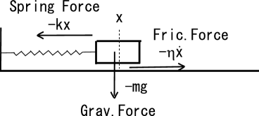
Figure 1: The harmonic oscillator with friction, (17b).

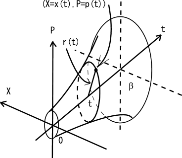
Figure 2: The two dimensional surface, (22b), in 3D bulk space (X,P,t).

References [1] N. Kikuchi, ”Nematics-Mathematical and Physical Aspects”, eds. J. -M. Coron, J. -M. Ghidaglia and Hélein, NATO Adv. Sci. Inst. Ser. C: Math. Phys. Sci. 332, Kluwer Acad. Pub., 1991, p195; [2] S. Ichinose, J.Phys:Conf.Ser.258(2010)012003, arXiv:1010.5558; [3] S. Ichinose, arXiv:1004.2573; [4] S. Ichinose, Prog.Theor.Phys.121(2009)727, ArXiv:0801.3064v8; [5] S. Ichinose, ArXiv:0812.1263[hep-th]; [6] S. Ichinose, Int.Jour.Mod.Phys.24A(2009)3620 , arXiv:0903.4971; [7] S. Ichinose, J. Phys. : Conf.Ser.222 (2010)012048, ArXiv:1001.0222; [8] S. Ichinose, J. Phys. : Conf.Ser.384(2012)012028, ArXiv:1205.1316; [9] S. Ichinose, arXiv:1303.6616(hep-th)