Effects of Multi-Field Phantom Inflation in Big Rip

Abstract

In this paper we study the behavior of the multi-field in phantom inflation, when massive scalar fields work collectively, in which the scale factor is a power law. We evaluate its parameter values by applying certain constraints on our model parameters, and we investigate that before the Big Rip singularity occurs the universe is in phantom inflationary phase. Furthermore, we calculate these values for this period then compare with current observations of CMB, BAO and observational Hubble data. We find that results may be consistent with observations. This implies that in the dark-energy equation of state (EOS) parameter $\omega_{DE}$ at the Big Rip remains finite, with the divergence of pressure and dark energy density.

Keywords: Phantom power-law, Cosmology, Multi-field.

1 Introduction

Cosmological observations made, by end of the last century and at the beginning of this century, have conclusive evidence for late cosmic acceleration [1]. It is driven by an unknown fluid violating strong energy condition (SEC), such that $\omega<-\frac{1}{3}$, with $\omega$ being the ratio of pressure density to energy density. This exotic fluid is known as dark energy (DE). The phantom field, in which the parameter of the equation of state $\omega<-1$, has still gained increasingly attention [2], motivated by the study of dark energy, e.g. [3], [4], [5], [6], [7], [8],[9], [10], [11]. The actions obeying the Phantomlike behavior may be arise in supergravity [12], scalar tensor gravity [13], higher derivative gravity [14], braneworld [15], string theory [16], and other scenarios [17, 18], and also from quantum effects [19]. The visible universe driven by the phantom field will evolve to a singularity, in which the energy density become infinite at finite time, which is called the Big Rip, see Refs. [20], [21], [22], [23], [24], [25] for other future singularities.

Recently, the little rip scenario has been proposed [26], in which the current acceleration of universe is driven by the phantom field, the energy density increases without bound, but $\omega$ tends to $-1$ asymptotically and rapidly, and thus the rip singularity dose not occur within finite time, however, in little rip scenario, the universe arrives at the singularity only at infinite time.

The simplest recognition of phantom field is a normal scalar field with reverse sign in its dynamical term. This reverse sign results in that, behave differently from the evolution of normal inflation during the normal inflation, the phantom field during the phantom inflation will be driven by its potential climb up along its potential. With the use of General Relativity (GR)which based on Friedmann equations, it observed that phantom-dominated epoch of the universe goes faster, but ends up in the form of Big-Rip singularity in a finite future time [2]. Phantom dark energy fields are characterized by violating the main energy condition, $\rho+p>0$. Also the conservation equation has the striking consequence that the energy density increases with expansion and with condition $\omega<-1$ matter is called Phantom energy [27]. On the basis of observational data Caldwell noted that $EOS$ parameter $"\omega"$ has a very short range in the neighborhood of $\omega=-1$ with more likelihood to the side of $\omega<-1$. He found that this possibility could not be neglected for the dark energy fluid. Alternatively, a very good description of the evolution of universe, is discussed in [28, 29] and [30].

Here, we will argue that after a finite period of the Big Rip phase the universe might return the evolution of observational universe. However, it is possible that some times after the energy density of the phantom field arrives at a high energy level, or before the rip singularity of universe is arrived, the energy of field will be released, and the universe reheats, after which the evolution of hot big bang recurs. For phantom scalar field a power law cosmology is defined by the cosmological scale factor evolving as $t^{\beta}$, see Refs. [31].

In our model, when many massive fields work collectively to drive phantom inflationary phase under certain constraints is known as multi-field (Nfield) phantom cosmology, in which the scale factor is a power law. In addition, it is very interesting to generalize the above studies for Nfield phantom cosmology with various potentials remains open.

Here, we study a general behavior of Nfield phantom inflation with the scale factor given in terms of parameter $\beta$ with out any dimension. The modified form of the scale factor is $a(t)=a_{0}(({t_{s}-t})/({t_{s}-t_{0}}))^{\beta}$ in order to achieve the self-stability, where $t_{s}$ is a required positive reference time [28].

The field starts from near an unstable equilibrium (taken to be at the origin) and climb up the potential to a stable maxima. In the phantom model, the observable Big Rip occurs during the climb up of scalar field and its magnitude is at most of order $M_{p}$ the Planck mass.

The arrangement of remaining sections of this paper is as; in section $2$, we formulate the whole picture of phantom power-law cosmology for multi-field. In section $3$ we consider observational data to impose certain bounds to investigate results for the multi-field parameters, and finally, section $4$ is devoted for conclusion and discussion.

2 Nfield with Power-Law Expansion

In this section we present Phantom cosmology under power law expansion, when many fields are working collectively with $\phi_{i}$ is the $ith$ phantom scalar field. For the simplicity of our model, we assume the homogenous and isotropic Friedmann-Robertson Walker (FRW) background metric,

$$ds^{2}=-dt^{2}+a^{2}(t)\left[\frac{dr^{2}}{1-kr^{2}}+r^{2}d{\Omega_{2}}^{2}\right].$$ (1)

Where $a(t)$ is a scale factor of the universe, $\Omega_{2}$ is $2$-dimension unit sphere volume, $t$ is the cosmic time and $k$ represents the curvature of $3$-dimensional space with $k=1,0,-1$ corresponds to open, flat and closed universe respectively. Our model is given by the following action, see Refs. [32, 33]:

$$S=\int{d^{4}x}\sqrt{-g}\left[\frac{R}{16\pi{G}}+\sum_{i}\left[\frac{1}{2}{g^{\mu\nu}}{\partial_{\mu}{\phi_{i}}}{\partial_{\nu}{\phi_{i}}}-V_{i}(\phi_{i})\right]+L_{m}\right].$$ (2)

Which involves $N$ phantom scalar fields, where $R$ is the Ricci scalar, $V_{i}$ potential of $ith$ phantom field and $G$ the Newton gravitational constant. The Lagrangian $L_{m}$ stands for the total matter of the universe including (dark plus baryonic). Finally, we concentrate on small redshifts, therefore, we are neglected the radiation sector, with speed of light as unity [32].

We assume the flat geometry of the universe i.e. $k=0$, for this model, the $ith$ phantom field satisfies the equations,

$$H^{2}=\frac{1}{3M^{2}_{p}}{\sum_{i}}[\rho_{\phi_{i}}+\rho_{m_{i}}]{},$$ (3)

$$\ddot{\phi_{i}}+3H\dot{\phi_{i}}-V^{\prime}(\phi_{i})=0{},$$ (4)

where $H(t)={\dot{a}}/{a}$ is the Hubble parameter represents the expansion rate of the universe at time $t$ and $M_{p}=(8\pi G)^{-\frac{1}{2}}$ is the Planck mass. $H^{2}>0$ requires that in all case for phantom evolution $\dot{\phi}^{2}$ must be smaller than its potential energy. In the above expression $\rho_{\phi_{i}}$ and $p_{\phi_{i}}$ are the energy density and pressure of the $ith$ phantom scalar field respectively, which are different from normal inflations model, reads [34, 35],

$$\rho_{\phi_{i}}=-\frac{1}{2}{\dot{\phi_{i}}}^{2}+V_{i}(\phi_{i}).$$ (5)

$$p_{\phi_{i}}=-\frac{1}{2}{\dot{\phi_{i}}}^{2}-V_{i}(\phi_{i}).$$ (6)

By varying with respect to scalar, we obtain the evaluation equation:

$$\dot{\rho_{\phi_{i}}}+3H(p_{\phi_{i}}+\rho_{\phi{i}})=0.$$ (7)

After simplification Eq. (7) can be evaluated for multi-field as follows:

$$\sum_{i}{\ddot{\phi}_{i}}+3H\sum_{i}{\dot{\phi}_{i}}-\sum_{i}\frac{dV_{i}}{d\phi_{i}}=0.$$ (8)

As in phantom cosmology the dark energy sector is attributed to the phantom fields, and thus its equation-of-state parameter is given by

$$\omega_{DE}=\frac{p_{DE}}{\rho_{DE}}=\frac{p_{\phi}}{\rho_{\phi}}.$$ (9)

And for matter-dominated universe, we have expression

$$\omega_{m_{i}}=\frac{p_{m_{i}}}{\rho_{m_{i}}}.$$ (10)

Finally, in the case of matter density, Eq. (7) becomes

$$\dot{\rho_{m_{i}}}+3H(1+\omega_{m_{i}})\rho_{m_{i}}=0,$$ (11)

with the simple form of its solution for multi-field is

$$\sum_{i}\rho_{m_{i}}=\rho_{m_{0}}\sum_{i}({\frac{1}{a^{n_{i}}}}),$$ (12)

where $n_{i}=3(1+\omega_{m_{i}})$ and here, we are dealing only with massive scalar fields, but the case of massless scalar fields are neglected in this regime. With the help of Eqs. (5) and (6), Eq. (4) can calculate the result for Nfield as

$$\dot{H}=\frac{1}{6M^{2}_{p}}\left[3\sum_{i}{\dot{\phi}_{i}^{2}}-\sum_{i}{\rho_{m_{i}}}n_{i}\right].$$ (13)

This result is consistent with single field inflation model when $N=1$, where $N$ stands for number of field. When we are working with Phantom cosmology, we replace $t$ by $t_{s}-t$; the reference time $t_{s}$ is sufficiently positive, then we obtain the scale factor by

$$a(t)=a_{0}{\left(\frac{t_{s}-t}{t_{s}-t_{0}}\right)}^{\beta},$$ (14)

with the Hubble parameter and its derivatives with respect to time is

$$H(t)=\frac{-\beta}{(t_{s}-t)},$$ (15)

$$\dot{H(t)}=-\frac{\beta}{(t_{s}-t)^{2}}.$$ (16)

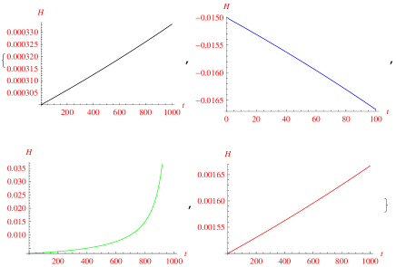
Figure 1: The evolution of $H$, the upper-left sketch corresponds to the parametrization of $(15)$ for $\beta=-3$, $t_{s}>t$, the upper-right sketch corresponds to the parametrization of $(15)$ for $\beta=15$, $t_{s}>t$, the lower-left sketch corresponds to the parametrization of $(15)$ for $\beta=-3$, $t_{s}=t$ and the lower-right sketch corresponds to the parametrization of $(15)$ for $\beta=-15$, $t_{s}>t$,

Now we investigate the behavior of universe which is depending on the value of $\beta$, thus for the value of $\beta$ less than zero, we observe an accelerating $(\ddot{a}(t)>0)$ universe and expanding $(\dot{a}(t)>0)$ universe, we find that $\dot{H(t)}$ is positive therein, which implies that it provides super acceleration, this is only possible for phantom power-law cosmology case. In addition, for the exponent $\beta<0$, and at late time $t=t_{s}$, as shown in Figure $1$, the scale factor $a(t)$ and Hubble parameter $H(t)$ of the universe both diverge as a result it goes to a Big Rip.
Such actions are common in phantom cosmology and their realization is a self-consistency test of our work, however, the important point which is already discussed in Ref. [36].

By using Eqs. (3) and (5) in Eq. (13), we find the potential $\langle V(t)\rangle=(\sum_{i}V_{i})/N$ which is the average value of $V_{i}(t)$ . Since $n_{i}=3(1+\omega_{m_{i}});\;\ 1\leq i\leq N$. For dust dominated universe $\omega_{mi}\rightarrow 0$, this implies that $n_{i}=3$ and as a result we obtain $\sum_{i}n_{i}=3N$. Therefore, it is given by

$$\langle V(t)\rangle=\frac{\sum_{i}V_{i}(t)}{N}=\left[M_{p}^{2}\left(\frac{3\beta^{2}-\beta}{(t_{s}-t)^{2}}\right)-\frac{5}{6}\frac{\rho_{m_{0}}}{{a_{0}}^{3}}\left(\frac{t_{s}-t_{0}}{t_{s}-t}\right)^{3{\beta}}\right].$$ (17)

From Eq. (13) we can obtain

$$\langle{{\dot{\phi}}(t)}^{2}\rangle=\left[\frac{-2\beta{M_{p}^{2}}}{(t_{s}-t)^{2}}+\frac{\rho_{m_{0}}}{{a_{0}}^{3}}\left(\frac{t_{s}-t_{0}}{t_{s}-t}\right)^{3{\beta}}\right].$$ (18)

Using the values from Eqs. (17) and (18) in Eq. (5)

$$\langle\rho_{\phi}\rangle=\left[M_{p}^{2}{\frac{3\beta^{2}}{(t_{s}-t)^{2}}}-\frac{4\rho_{m_{0}}}{3{a_{0}}^{3}}\left(\frac{t_{s}-t_{0}}{t_{s}-t}\right)^{3{\beta}}\right].$$ (19)

Again putting Eqs. (17) and (18) into Eq. (6) we get

$$\langle p_{\phi}\rangle=\left[M_{p}^{2}\frac{(-3\beta^{2}-\beta+3\beta)}{(t_{s}-t)^{2}}+(t_{s}-t)H(t)+\frac{\rho_{m0}}{3{a_{0}}^{3}}\left(\frac{t_{s}-t_{0}}{t_{s}-t}\right)^{3{\beta}}\right].$$ (20)

In the case of phantom Nfield, the dark energy equation-of-state parameter is

$$\omega_{DE}(t)={p_{\phi}}/{\rho_{\phi}},$$

which implies that

$$w_{DE}(t)=(-1+{\frac{1}{\beta}}).$$ (21)

We see that for Big Rip behavior, $\omega_{DE}(t)$ always having finite value [20].
For $\beta$ less than zero possesses additionally a positive $\dot{H(t)}$ that leads to super-acceleration [37]. So such kind of scenario expansion is always came with acceleration. From Eq. (21), for $\omega<0$ we come to know that the value of $\omega$ is very narrow to phantom divide.
Furthermore, with the value of $\beta$ less than zero, at $t$ equal to $t_{s}$ the scale factor and the Hubble parameter diverge, that is the universe results to a Big Rip. We investigate that these behaviors of Nfield phantom cosmology are very similar with result of single field phantom cosmology with power-law [36]. Here, we have limited the parameter $\beta$ small, however, it is interesting to consider the phenomena of $\beta\gg 1$, i.e. there is a new step, by which the density of dark energy observed might be linked to that of inflation, as in the eternal expanding cyclic scenario.

3 A Bound for $N$ for Nfield and Fit the Observational Data

In this section, we apply the techniques that conform the values of multi-field with the observational data. Now we are fitting the observational data, presenting our results in the case of many fields are working collectively. We observed that our values for all parameters in Table I are best fitted with minor error of accuracy, which is negligible for large scale, we also provide the $1\sigma$ bound of every parameter. Similarly in Table II we present the maximum possibility of the values up to $1\sigma$ bound for the derived parameters, namely the power-law exponent $\beta$, the present matter energy density value $\rho_{m_{0}}$, the present critical energy density value $\rho_{c_{0}}$ and the Big Rip time $t_{s}$. As we observed that $\beta$ is always less than zero, as expected in consistent phantom cosmology.

Furthermore, we observed that the Big Rip time is one order of magnitude greater than the present age of the universe, which shows that such an outcome is predictable in phantom cosmology, unless one include additional mechanisms as shown in Ref. [38].

$$\langle V(t)\rangle\simeq\left[{\frac{6.5\times 10^{27}}{{(3.30\times 10^{18}-t})^{2}}\large}-2.52\times 10^{-371}\times(3.30\times 10^{18}-t)^{19.54}\right].$$ (22)

While when we consider $WMAP7$ data alone, it provides

$$\langle V(t)\rangle\simeq\left[{\frac{6.41\times 10^{27}}{{(3.30\times 10^{18}-t})^{2}}\Large}-1.98\times 10^{-369}\times(3.30\times 10^{18}-t)^{19.37}\right].$$ (23)

Here we noted that in above results although the second term is very small at early times of the universe, but becomes very important at late times, this situation is close to the Big Rip. Now the scalar field evolution at late time $(t\rightarrow t_{s})$, $\rho_{m_{0}}$ can be neglected and also set $a_{0}=1$.
Thus we obtain the new results for Nfield in phantom cosmology as follows:

$${\dot{\phi}}=\sqrt{\sum_{i}(\dot{\phi}_{i})^{2}}\simeq{\frac{\sqrt{-2N\beta}{M_{p}}}{(t_{s}-t)}},$$ (24)

which implies that

$$\phi(t)\simeq{\sqrt{-2N\beta}{M_{p}}}\ln|{t_{s}-t}|.$$ (25)

Thus the result is similar with single field Phantom model when $N=1$ see [36]. However for large field we can find some new interesting results for future. Additionally, the total change of all fields is determined by the radial motion in field space ( for example see Ref. [35]), we have

$$\Delta\phi\simeq{\frac{\sqrt{\sum_{i}({\dot{\phi}_{i}})^{2}}}{H}}\simeq-\sqrt{{\frac{-2N}{\beta}}}M_{p}.$$ (26)

Thus we see that for $\beta<-1$, the total absolute change of all fields is directly proportional to the square root of $N$ and inversely proportional to square root value of exponent $\beta$, for the value $\beta=0$, this change is undefined, which is not possible in Phantom cosmology.
Furthermore, for the combined $WMAP7+BAO+H_{0}$, which implies that

$$\phi(t)\cong{{\sqrt{N}}}[({-2.645\times 10^{13}}).\ln|{3.30\times 10^{18}-t}|],$$ (27)

while single $WMAP7$ data provides that

$$\phi(t)\cong{{\sqrt{N}}}[({-2.643\times 10^{13}}).\ln|{3.30\times 10^{18}-t}|].$$ (28)

According to our exactions the phantom field and the kinetic energy diverge at the Big Rip time.

  Parameter $$H_{0}+WMAP7+BAO$$   WMAP7

TABLE I: Observational maximum likelihood values in $1\sigma$ confidence level has taken from [39].

  Parameter $$H_{0}+WMAP7+BAO$$   WMAP7

TABLE II: Derived maximum likelihood values in $1\sigma$ confidence level for the power-law exponent, present value of critical energy density, present matter density, and $t_{s}$ at Big Rip time.

4 Conclusion and Discussion

In Big Rip phase, $\omega<-1$, the energy density of the all phantom field together will increase with time, and arrive at a high energy scale at finite time, and at this epoch the phantom field has $\omega\simeq-1$. Here, we actually required that before $\omega\simeq-1$, the phantom field must have arrived at a high energy regime, which assures the occurrence of inflation. However, the some Phantom fields loose their energy and jump back, this process is continuous and inflation never goes to end, such type is known as eternal phantom inflation which will be shown in later work.

In this paper, we study the Nfield phantom model, in which collection of massive scalar fields drive it in early time of universe. Now from Eq. (27) and Eq. (28), we find the different values of $t$ and put them in Eq. (22) and Eq. (23), to evaluate the average value of potential for the Nfield Phantom power-law i.e. $\langle V(\phi)\rangle$.

Thus, for the $WMAP7+BAO+H_{0}$ , the potential is fitted as

$$\langle V(\phi)\rangle\approx[{6.48\times 10^{27}}e^{0.77\times 10^{-13}({\phi}/\sqrt{N})}-2.52\times 10^{-371}e^{-7.44\times 10^{-13}({\phi}/\sqrt{N})}],$$

and while for $WMAP7$, we can find

$$\langle V(\phi)\rangle\approx[{6.39\times 10^{27}}e^{0.78\times 10^{-13}({\phi}/\sqrt{N})}-1.98\times 10^{-369}e^{-7.5\times 10^{-13}({\phi}/\sqrt{N})}],$$

respectively.

In our study of multi-field phantom cosmology, we observed that the cosmic scale factor $a(t)$ is obeying the power law, for $N=1$, it will give the result similar to single field, but when $N$ is very very large, the value of $V(\phi)$ vary between $4\times 10^{27}$ to $5.41\times 10^{27}$. When we construct the whole scenario, we fit the observationally data of $WMAP7+BAO+H_{0}$ and $WMAP7$ alone by applying bound on the multi-field by focusing on exponent $\beta$ and the Big Rip time $t_{s}$. By using separately WMAP7 data, we obtained the value $\beta\cong{-6.523\pm 0.38}$, while the Big Rip is observed at $t_{s}\cong 102.8\pm 3.475\;Gyr$.
However, the dark energy equation of state parameter $\omega_{DE}$ lies below the phantom divide, it was expected and at Big Rip time it always remains finite and nearly equal to $-1.1533$. Although the phantom dark anergy density and pressure are diverging behavior at the Big Rip. By using $WMAP7+BAO+H_{0}$ data set alone we find $\beta\approx{-6.51_{+{0.24}}^{-0.25}}$, while the Big Rip is observed at $t_{s}\approx 104.5_{+{1.9}}^{-2.0}~{}Gyr$, in $1\sigma$ confidence level. Definitely, the subject of Nfield quantization of such scenarios is open and needs further investigation on this.

5 Acknowledgment

We thank Yun-Song Piao for useful discussions and comments.We also thank HEC (Higher Education Commission Pakistan) for providing the facilities to carry out the research work.

References

- [1] S.J. Perlmutter et al., Astrophys. J. 517,565 (1999); D.N. Spergel et al., Astrophys. J. Suppl. 148 175 (2003); G. Calcagni, Phys. Rev. D69, 103508 (2004).
- [2] R.R. Caldwell, Phys. Lett. B545, 23 (2002)
- [3] R.R. Caldwell, M. Kamionkowski and N.N. Weinberg, Phys. Rev. Lett. 91, 071301 (2003).
- [4] P. Singh, M. Sami and N. Dadhich, Phys. Rev. D68, 023522 (2003); M. Sami and A. Toporensky, Mod. Phys. Lett. A19, 1509 (2004).
- [5] J.G. Hao, X.Z. Li, Phys. Rev. D67, 107303 (2003).
- [6] S. Nojiri, S.D. Odintsov, Phys. Lett. B562, 147 (2003); E. Elizalde, S. Nojiri, S.D. Odintsov, Phys. Rev. D70, 043539 (2004).
- [7] Z.K. Guo, Y.S. Piao, and Y.Z. Zhang, Phys. Lett. B594, 247 (2004).
- [8] J.M. Aguirregabiria, L.P. Chimento, R. Lazkoz, Phys. Rev. D70, 023509 (2004); L.P. Chimento, D. Pavon, Phys. Rev. D73, 063511 (2006).
- [9] Kujat, R.J. Scherrer, A.A. Sen, Phys. Rev. D74 083501 (2006).
- [10] V. Faraoni, Class. Quant. Grav. 22, 3235 (2005); J.V. Faraoni, A. Jacques, Phys. Rev. D76, 063510 (2007).
- [11] K. Bamba, C.Q. Geng, Prog. Theor. Phys. 122, 1267 (2009); K. Bamba, M. Jamil, D. Momeni, R. Myrzakulov, arXiv:1203.2103; K. Bamba, K. Yesmakhanova, K. Yerzhanov, R. Myrzakulov, arXiv:1203.3401.
- [12] H.P. Nilles, Phys. Rept. 110 1 (1984).
- [13] B. Boisscau, G. Esposito-Farese, D. Polarski and A.A. Starobinsky, Phys. Rev. lett. 85 2236 (2000).
- [14] M.D. Pollock, Phys. Lett. B215, 635 (1988).
- [15] V. Sahni and Y. Shtanov, JCAP 0311, 014 (2003).
- [16] P. Frampton, Phys. Lett. B555, 139 (2003).
- [17] L.P. Chimento and R. Lazkoz, Phys. Rev. Lett. 91 211301 (2003).
- [18] H. Stefancic, Eur. Phys. J. C36, 523 (2004).
- [19] V.K. Onemli, R.P. Woodard, Class. Quant. Grav. 19, 4607 (2002); V.K. Onemli, R.P. Woodard, Phys. Rev. D70, 107301 (2004); E.O. Kahya, V.K. Onemli, Phys. Rev. D76, 043512 (2007); E.O. Kahya, V.K. Onemli, and R.P. Woodard, Phys. Rev. D81, 023508 (2010).
- [20] S. Nojiri, S.D. Odintsov, S. Tsujikawa, Phys. Rev. D71, 063004 (2005).
- [21] J.D. Barrow, Class. Quant. Grav. 21, L79 (2004); Class. Quant. Grav. 21, 5619 (2004).
- [22] H. Stefancic, Phys. Rev. D71, 084024 (2005).
- [23] I.H. Brevik, O. Gorbunova, Gen. Rel. Grav. 37, 2039 (2005).
- [24] M.P. Dabrowski, Phys. Lett. B625, 184 (2005).
- [25] M. Bouhmadi-Lopez, P.F. Gonzalez-Diaz, P. Martin- Moruno, Phys. Lett. B659, 1 (2008).
- [26] P.H. Frampton, K.J. Ludwick, R.J. Scherrer, Phys. Rev. D84, 063003 (2011).
- [27] A. Liddle “An Introduction to Modern Cosmology” (Second Edition) (2003).
- [28] S. Nojiri and S.D. Odintsov, Gen. Rel. Grav. 38, 1285 (2006); I.P. Neupane and H. Trowland, arXiv:0902.1532; I. P. Neupane and C. Scherer, JCAP 0805, 009 (2008).
- [29] E. W. Kolb, Astrophys. J. 344, 543 (1989).
- [30] M. Jamil, A. Qadir, Gen. Rel. Grav. 43, 1069-1082 (2011)
- [31] A. Dev, D. Jain and D. Lohiya , arXiv:0804.3491v1 (2008).
- [32] R. R. Caldwell, Phys. Lett. B 545, 23 (2002); P. Singh, M. Sami and N. Dadhich, Phys. Rev. D 68, 023522 (2003); J. M. Cline, S. Jeon and G. D. Moore, Phys. Rev. D 70, 043543 (2004); V. K. Onemli and R. P. Woodard, Phys. Rev. D 70, 107301 (2004); W. Hu, Phys. Rev. D 71, 047301 (2005); M. R. Setare and E. N. Saridakis, JCAP 0903, 002 (2009); E. N. Saridakis, Nucl. Phys. B 819, 116 (2009); S. Dutta and R. J. Scherrer, Phys. Lett. B 676, 12 (2009).
- [33] Y.F. Cai and W. Xue, Phys. Lett. B 680, 395-398 (2009).
- [34] I. Ahmad, Y.S. Piao and C.F. Qiao, JCAP 0802, 002 (2008).
- [35] I. Ahmad, Y.S. Piao and C.F. Qiao, JCAP 0806, 023 (2008).
- [36] C. Kaeonikhom , B. Gumjudpai and E.N. Saridakis, Phys. Lett. B 695, 45-54 (2011)
- [37] S. Das, P. S. Corasaniti and J. Khoury, Phys. Rev. D 73, 083509 (2006); M. Kaplinghat and A. Rajaraman, Phys. Rev. D 75, 103504 (2007).
- [38] M. Sami and A. Toporensky, Mod. Phys. Lett. A 19, 1509 (2004);
- [39] E. Komatsu et al. arXiv:1001.4538v3 (2011).