PTF11agg as the First Evidence for Reverse Shock Emission from a Postmerger Millisecond Magnetar

Abstract

Based on the stiff equations of state of neutron stars (NS) and the discovery of high-mass NSs, a NS-NS merger will leave behind, with high probabilities, a rapidly rotating massive magnetar. The central magnetar will dissipate its rotational energy to the outflow by injecting Poynting flux, which will become lepton-dominated so that a long-lasting reverse shock (RS) is developed. We calculate the emission of the RS as well as the emission of forward shock (FS) and find that in most cases the RS emission is stronger than FS emission. It is found that the recently discovered transient, PTF11agg, can be neatly accounted for by the RS emission powered by a millisecond magnetar. Other alternative models have been considered and cannot explain the observed light curves well. We therefore suggest that PTF11agg be the first evidence for RS emission from a postmerger millisecond magnetar.

1 Introduction

When binary neutron stars (BNS) merge, a black hole is usually assumed to be formed (Faber & Rasio, 2012). With the theoretical work on stiff equations of state and the discovery of massive neutron stars (Lattimer, 2012), several authors (Dai et al., 2006; Zhang, 2013) suggest that a stable massive neutron star (NS) may be formed as a post-merger product. This suggestion is supported by numerical-relativity simulations (Hotokezaka et al., 2013; Giacomazzo & Perna, 2013). Because the newborn NSs are differentially rotating rapidly, the onset of magneto-rotational instability could boost the magnetic field of such NSs to magnetar levels (Duncan & Thompson, 1992; Kluźniak & Ruderman, 1998; Dai & Lu, 1998a). Energy injection from millisecond magnetars is also invoked to account for the unusual X-ray emission following some short gamma-ray bursts (SGRBs) (Dai et al., 2006; Fan & Xu, 2006; Rowlinson et al., 2010, 2013).

The electromagnetic signatures of NS-NS mergers include SGRBs (Eichler et al., 1989; Barthelmy et al., 2005; Gehrels et al., 2005; Rezzolla et al., 2011), radio afterglows (Nakar & Piran, 2011; Metzger & Berger, 2012; Rosswog et al., 2013; Piran et al., 2013), day-long optical macronovae (Li & Paczyński, 1998; Kulkarni, 2005; Rosswog, 2005; Metzger et al., 2010; Roberts et al., 2011; Metzger & Berger, 2012), and possible X-ray emissions (Palenzuela et al., 2013) due to the interaction of the NS magnetospheres during the inspiral and merger. Zhang (2013) recently suggested that, by the formation of rapidly spinning magnetars, there is a significant fraction of NS-NS mergers that may be detected as bright X-ray transients associated with gravitational wave bursts (GWBs) without apparent association of SGRBs. Subsequently, based on the energy injection scenario proposed by Dai & Lu (1998b), Gao et al. (2013) considered the rich electromagnetic signatures of the forward shock (FS) driven by ejecta subject to continuous injection of Poynting flux from the central magnetars.

We here consider the electromagnetic signatures not only of FS that was considered by Gao et al. (2013), but also of reverse shock (RS) because it is more likely that the magnetar wind would be dominated by ultra-relativistic leptons ($e^{+}e^{-}$ pairs) within radius $\sim 10^{17}\mathord{\thinspace\rm cm}$ (Dai, 2004; Coroniti, 1990; Michel, 1994).

The structure of this paper is as follows. In Section 2 we outline our model, analytical method, and results. Section 3 presents the numerical method and its application to the recently discovered transient source PTF11agg. In Section 4 we discuss other alternative models to interpret PTF11agg.

2 The Model

The basic picture of the model is illustrated in Figure 1 of Gao et al. (2013). The merger of BNSs ejects a mildly anisotropic outflow with typical velocity $0.1-0.3c$ and mass $M_{\mathrm{ej}}\sim 10^{-4}-10^{-2}M_{\odot}$ (Rezzolla et al., 2010; Hotokezaka et al., 2013; Rosswog et al., 2013). The onset of Poynting flux launched $\sim 10\mathord{\thinspace\rm s}$ later catches up the ejecta and crosses the ejecta in $t_{\Delta}\sim 3\mathord{\thinspace\rm s}L_{0,47}^{-1/2}\Delta_{7}^{1/2}M_{\mathrm{ej},-3}^{1/2}$ (Gao et al., 2013), where $L_{0}\equiv\xi L_{\mathrm{sd},0}$ is the power injected into the ejecta by the magnetar wind, $L_{\mathrm{sd},0}=1\times 10^{47}\mathord{\thinspace\rm erg}\mathord{\thinspace\rm s}^{-1}P_{0,-3}^{-4}B_{p,14}^{2}R_{6}^{6}$ is the luminosity of the central magnetar. Here we adopt the usual convention $Q=10^{n}Q_{n}$. The value of $\Delta\sim 10^{7}\mathord{\thinspace\rm cm}$ is just a reasonable suggestion and is unimportant here because our results do not depend on this value. It is known that the Poynting flux from the magnetar via magnetic dipole radiation is nearly isotropic. Thus, the Poynting flux will always catch up with the ejecta, though the latter could be asymmetric.

The dynamics of the blast wave is determined by

$$L_{0}\min\left(t,T_{\mathrm{sd}}\right)=\left(\gamma-\gamma_{\mathrm{ej},0}\right)M_{\mathrm{ej}}c^{2}+2\left(\gamma^{2}-1\right)M_{\mathrm{sw}}c^{2},$$ (1)

where $T_{\mathrm{sd}}$ is the spin-down time of the central magnetar in the observer frame, $M_{\mathrm{sw}}=\left(4/3\right)\pi r^{3}nm_{p}$ is the swept-up mass of the ambient medium (region 1), $\gamma\simeq\gamma_{3}$ is the Lorentz factor of the forward-shocked medium (region 2), $\gamma_{\mathrm{ej},0}$ is the initial Lorentz factor of the ejecta. In the analytical calculations, we set $\gamma_{\mathrm{ej},0}=1$, and in the numerical calculations discussed in Section 3 we set $\gamma_{\mathrm{ej},0}$ according to the typical initial velocity of the ejecta $\beta_{\mathrm{ej},0}\simeq 0.2$. Because the fraction of the total power is $\xi$ $\sim 0.8-0.9$ (Zhang, 2013), we will approximate it as $\xi\approx 1$ in the following calculation. Equation $\left(\ref{dynamics}\right)$ is different from equation (1) of Gao et al. (2013) by a factor 2 in the second term on the right hand side because the injected energy is deposited both in FS and in RS and the energy contained in FS and RS is comparable (Blandford & McKee, 1976).

The FS emission is calculated quantitatively similar to that derived by Gao et al. (2013). The energy density and number density of the reverse-shocked wind (region 3) is determined by (Sari & Piran, 1995; Blandford & McKee, 1976) $e_{3}/(n_{3}m_{e}c^{2})=\bar{\gamma}_{3}-1\simeq\bar{\gamma}_{3}$ and $n_{3}/n_{4}=4\bar{\gamma}_{3}+3\simeq 4\bar{\gamma}_{3}$ with $n_{4}=L_{0}/4\pi r^{2}\gamma_{4}^{2}m_{e}c^{3}$, where $\gamma_{4}$ is the Lorentz factor of the unshocked wind (region 4). The minimum Lorentz factor of the $e^{+}e^{-}$ in region 3 is (Sari et al., 1998) $\gamma_{3m}=\epsilon_{e}[(p-2)/\left(p-1\right)]\bar{\gamma}_{3}$, where a constant fraction $\epsilon_{e}$ (subject to the condition $\epsilon_{e}+\epsilon_{B}=1$) of the shock energy goes into $e^{+}e^{-}$ so that the magnetic field of region 3 is determined by $B_{3}=\left(8\pi\epsilon_{B}e_{3}\right)^{1/2}$ (Sari et al., 1998). The self-absorption frequency $\nu_{a}$ is calculated according to Wu et al. (2003).

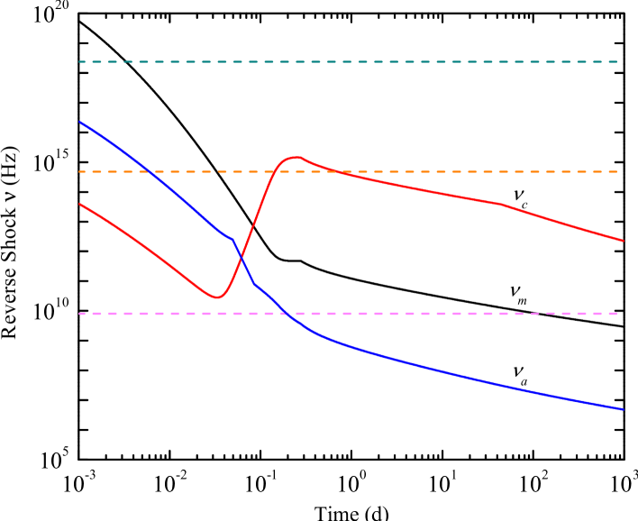
Figure 2: Characteristic frequencies of PTF11agg (Numerical results). The three dashed lines mark radio (8 $\mathord{\thinspace\rm GHz}$), optical ($R$) and X-ray bands, respectively.

Before the FS becomes relativistic, the slow expansion of the ejecta implies a large $\bar{\gamma}_{3}\simeq\gamma_{4}$. Therefore $e^{+}e^{-}$ in region 3 are very hot, resulting in high X-ray flux, which will last for several hundred seconds before optical emission takes over. The continuous energy injection will maintain the optical flux to a relatively high level until the time $T_{\mathrm{sd}}$. During this process, radio emission becomes progressively dominated and could last for years before rapid decline. At time $T_{\mathrm{sd}}$, the central engine turns off and region 4 disappears, thereafter region 3 begins to spread linearly, i.e., the width of region 3 in comoving frame $\Delta_{3}\propto r$. Additionally, because the $e^{+}e^{-}$ are in slow cooling regime after $T_{\mathrm{sd}}$ (see Figure 2), $\gamma_{3m}$ is essentially constant thereafter.

Gao et al. (2013) discussed four cases depending on different parameter configurations. Here we consider only Case I in their paper, viz. the case $T_{\mathrm{dec}}<T_{\mathrm{sd}}$. We find that the optical transient PTF11agg (Cenko et al., 2013) can be neatly interpreted according to RS emission powered by a millisecond magnetar (Figure 3).

Here we first list the corresponding timescales and Lorentz factor at $T_{\mathrm{dec}}$ that are similar to that derived by Gao et al. (2013):

$$T_{\mathrm{N1}} = 2.1\times 10^{-2}\mathord{\thinspace\rm d}L_{0,47}^{-1}M_{\mathrm{ej},-4}$$ (2)

$$T_{\mathrm{dec}} = 0.28\mathord{\thinspace\rm d}L_{0,47}^{-7/10}M_{\mathrm{ej},-4}^{4/5}n^{-1/10}$$ (3)

$$T_{\mathrm{N2}} = 2.4\times 10^{2}\mathord{\thinspace\rm d}L_{0,47}^{1/3}T_{\mathrm{sd},5}^{1/3}n^{-1/3}$$ (4)

$$\gamma_{\mathrm{dec}} = 6.7L_{0,47}^{3/10}M_{\mathrm{ej},-4}^{-1/5}n^{-1/10}+1,$$ (5)

where we use day instead of second as the units of time to ease comparison with the observational data (Figure 1 and 3). Here $T_{\mathrm{N1}}$ and $T_{\mathrm{N2}}$ are the times $\gamma-1=1$, viz. the transition times between relativistic and Newtonian dynamics, $T_{\mathrm{dec}}$ is the deceleration time whereafter the blast wave begins to decelerate. It can be seen that the above analytically derived values are in good agreement with the numerical results (Figure 1) except for $T_{\mathrm{N2}}$, which could be overestimated by one magnitude. The reason is that we set the radius $r_{\mathrm{N2}}=cT_{\mathrm{N2}}$ in the analytical calculations. This approximation significantly underestimates the actual radius because of the prominent relativistic time propagation effect (Zhang & Mészáros, 2004) before $T_{\mathrm{N2}}$. A better approximation is to take $r_{\mathrm{N2}}=4\bar{\gamma}^{2}cT_{\mathrm{N2}}$ with the average Lorentz factor $\bar{\gamma}$ lying between $1$ and $\gamma_{\mathrm{dec}}$.

The temporal scaling indices of various parameters are listed in Table 1. From Figure 2 and Table 1 we see that there are three more times that shape the temporal evolution of the corresponding parameters and lightcurves:

$$T_{\mathrm{ct}} = 6.0\times 10^{-2}\mathord{\thinspace\rm d}L_{0,47}^{-2/3}M_{\mathrm{ej},-4}^{5/6}\epsilon_{B,-1}^{1/6}$$ (6)

$$T_{ac} = 0.11\mathord{\thinspace\rm d}L_{0,47}^{-\left(8p+25\right)/2\left(6p+19\right)}M_{\mathrm{ej},-4}^{\left(5p+16\right)/\left(6p+19\right)}\epsilon_{B,-1}^{\left(2p+5\right)/2\left(6p+19\right)}\gamma_{4,4}^{-1/\left(6p+19\right)}$$ (7)

$$T_{mc} = 0.13\mathord{\thinspace\rm d}L_{0,47}^{-5/7}M_{\mathrm{ej},-4}^{6/7}\epsilon_{B,-1}^{1/7}\epsilon_{e}^{1/7}\gamma_{4,4}^{1/7},$$ (8)

where $T_{ac}$ and $T_{mc}$ are the respective crossing time of $\nu_{c}$ with $\nu_{a}$ and $\nu_{m}$. More words are needed for $T_{\mathrm{ct}}$. Owing to the brake caused by the massive ejecta, the magnetar wind cannot drive the ejecta to large radius at beginning, resulting in high energy density and therefore strong magnetic field of region 3. Consequently, the $e^{+}e^{-}$ cool so fast that the cooling Lorentz factor (Sari et al., 1998) $\gamma_{c}\approx 1$. Only after $T_{\mathrm{ct}}$ does $\gamma_{c}$ deviate significantly from 1. So $T_{\mathrm{ct}}$ is defined by the condition $3\pi m_{e}c=\sigma_{T}\gamma B_{3}^{2}T_{\mathrm{ct}}$.

The various frequencies of the RS emission at $T_{\mathrm{dec}}$ are

$$\nu_{a,\mathrm{dec}} = 1.8\times 10^{10}\mathord{\thinspace\rm Hz}L_{0,47}^{51/50}M_{\mathrm{ej},-4}^{-12/25}\epsilon_{B,-1}^{1/5}\epsilon_{e}^{-1}\gamma_{4,4}^{-8/5}n^{13/50}\frac{p-1}{p-2}\left[\frac{p+2}{p+\frac{2}{3}}\left(p-1\right)\right]^{3/5}$$ (9)

$$\nu_{m,\mathrm{dec}} = 9.9\times 10^{12}\mathord{\thinspace\rm Hz}\epsilon_{B,-1}^{1/2}\epsilon_{e}^{2}\gamma_{4,4}^{2}n^{1/2}\left(\frac{p-2}{p-1}\right)^{2}$$ (10)

$$\nu_{c,\mathrm{dec}} = 5.1\times 10^{14}\mathord{\thinspace\rm Hz}L_{0,47}^{1/5}M_{\mathrm{ej},-4}^{-4/5}\epsilon_{B,-1}^{-3/2}n^{-9/10}$$ (11)

$$F_{\nu,\max,\mathrm{dec}} = 5.6\times 10^{3}\mathord{\thinspace\rm mJy}L_{0,47}^{9/10}M_{\mathrm{ej},-4}^{2/5}\epsilon_{B,-1}^{1/2}\gamma_{4,4}^{-1}n^{1/5}D_{27}^{-2}.$$ (12)

3 Numerical Approach and the Transient Source PTF11agg

Recently, the wide-field survey telescope Palomar Transient Factory (PTF) reported the discovery of a transient source, PTF11agg, of very unusual nature (Cenko et al., 2013). PTF11agg consists of a bright, rapidly fading optical transient of two days long and an associated year-long scintillating radio transient, without a high-energy trigger. It is demonstrated that a galactic origin of such a transient is ruled out (Cenko et al., 2013). We inspect the observed properties and lightcurves of PTF11agg and speculate that this transient could be the first evidence for RS emission powered by a magnetar.

There are several lines of reasoning for this speculation. First, a magnetar wind can power the optical RS emission until $T_{\mathrm{sd}}$, which is typically 1 day. Second, the duration of radio emission of PTF11agg is in accord with our estimate of the duration of radio RS emission powered by a millisecond magnetar. Third, the energy scale of the blast wave of PTF11agg is just the same as the rotational energy of a millisecond magnetar. It is measured by means of interstellar scattering and scintillation that PTF11agg had an angular diameter of $\Theta\approx 20\mathord{\thinspace\rm\mu as}$ at observer’s time $\Delta t_{\mathrm{obs}}\approx 100$ days. By this time the emitting source should be in the transrelativistic or Newtonian regime so that the Sedov-Taylor energy is approximately applicable, $E_{0}=(4/3)\pi r^{3}nm_{p}c^{2}$. Adopting the typical values $n\simeq 1\mathord{\thinspace\rm cm}^{-3}$ and $z\simeq 1$, we estimate the total energy injected to be $\sim 10^{52}\mathord{\thinspace\rm erg}$, i.e., the energy scale of a typical millisecond magnetar. Fourth, although the simplest on-axis long GRB (LGRB) afterglow explanation proposed by Cenko et al. (2013) cannot be ruled out at this time, we will see (Figure 3) that the magnetar model proposed in this paper provides a much better fit to the data with more reasonable fitting parameters.

Based on the above lines of reasoning, we perform numerical calculations as well as analytical calculations presented above. In our numerical calculations, we first solve equation $\left(\ref{dynamics}\right)$ for $\gamma$, from which the velocity of the ejecta can be got. We then precede to accumulatively calculate the radius of the shock front. $M_{\mathrm{sw}}$, $n_{4}$ and other quantities are then calculated straightforwardly. Because we do not know a priori the redshift of the source, we just guess a redshift in the range $0.5\lesssim z\lesssim 3.0$ as constrained by Cenko et al. (2013). Then we determine a group of parameters that best fit the data for such a redshift. If the resulting size of the blast wave at $\Delta t_{\mathrm{obs}}\approx 100$ days does not satisfactorily give the measured angular size, we guess another redshift until a self-consistent fitting is found. In passing, although we do not bother to include the redshift $z$ in equations listed above, we do include it in the numerical calculations.

The initial radius of the swept region is set to $r_{0}=6\times 10^{10}\mathord{\thinspace\rm cm}$ which is the distance the ejecta, with a typical velocity $v\approx 0.2c$, traveled before the magnetar wind is launched (Gao et al., 2013). The numerically determined best-fit lightcurves are depicted in Figure 3 with the analytical result marked piecewisely. The best-fit parameters are listed in Table 2. In Figure 3 we do not include the two points (standing for a faint quiescent optical counterpart) in the optical lightcurve at later times (i.e., $t>10\mathord{\thinspace\rm days}$, see Figure 6 of Cenko et al., 2013) because by these times the optical flux coming from the transient source fell below $0.1\mathord{\thinspace\rm\mu Jy}$ so that the faint quiescent optical counterpart stood out. We find that the magnetar wind was launched at $t_{0}=0$:55:06 on 2011 January 30, i.e., $4.368$ hours before the first image was taken at 5:17:11 on the same day (Cenko et al., 2013). This launch time is more than 1 hour later than determined by Cenko et al. (2013), resulting in a shallower optical decay index.

From Table 2 we see that $M_{\mathrm{ej}}=1.2\times 10^{-4}M_{\odot}$, consistent with the numerical simulations (Rezzolla et al., 2010). The luminosity $L_{0}$ and the local frame spin down timescale $T_{\mathrm{sd}}/\left(1+z\right)$ of the magnetar give the initial rotation period of the magnetar $P_{0}=3.1\mathord{\thinspace\rm ms}$ in local frame and the dipole magnetic field $B_{p}=2.0\times 10^{15}\mathord{\thinspace\rm G}$ for the typical values $R_{6}=1$ and $I_{45}=1.5$. The derived $P_{0}=3.1\mathord{\thinspace\rm ms}$ lies between the minimum rotation period of a stable NS $P_{\mathrm{crit}}\sim 1\mathord{\thinspace\rm ms}$ and the maximum rotation period $P_{\mathrm{dyn}}\sim 5\mathord{\thinspace\rm ms}$ when the $\alpha$-$\Omega$ dynamo action quickly builds up the magnetic field before the NS dissipates its internal heat via cooling (Duncan & Thompson, 1992; Thompson & Duncan, 1993). $\gamma_{4}=4.6\times 10^{4}$ is consistent with the value derived for the Crab pulsar (Atoyan, 1999; Dai, 2004). The inferred circumburst density $n=0.13\mathord{\thinspace\rm cm}^{-3}$ is consistent with the findings by other studies (Berger et al., 2005; Soderberg et al., 2006; Berger, 2007). In contrast, the circumburst density for LGRBs is usually higher than for SGRBs. This strengthens the argument that PTF11agg was a circum-binary transient rather than a LGRB afterglow considered by Cenko et al. (2013) because they inferred $n\sim 10^{-3}\mathord{\thinspace\rm cm}^{-3}$. We therefore conclude that the best-fit values are all well within the reasonable ranges.

Figure 3 shows that the temporal decay indices of optical flux and radio flux both depend on the parameter $p$. This same parameter also sensitively determines the time $T_{m,\mathrm{rad}}$ when $\nu_{m}=\nu_{\mathrm{rad}}$ because $\nu_{m}\propto\left[\left(p-2\right)/\left(p-1\right)\right]^{2}$. In the numerical calculations we find that $p$ is accurately determined as $p=2.2$, any deviation of even $0.05$ would significantly modify the resulting lightcurves so as not to fit the data closely. $T_{\mathrm{sd}}$ is also accurately determined as can be seen from the optical lightcurve in Figure 3. To get a satisfactory fit, $n$ cannot deviate from the given value by more than $0.08$. The only loosely constrained value is $\epsilon_{B}$, for which a deviation of $0.05$ is also acceptable. But too large a value of $\epsilon_{B}\sim 0.2$ is not favored by the data.

Figure 3 shows that the radio flux suffered from a rapid decline, with a temporal decay index $\alpha=3\left(p+1\right)/10\simeq 1$, after the time $T_{m,\mathrm{rad}}\approx 113$ days. Before $T_{m,\mathrm{rad}}$ the derived radio spectral index $\beta=1/3$ is consistent with the observations (see Figure 4 of Cenko et al., 2013). We infer $\gamma=1.9$ at $\Delta t_{\mathrm{obs}}\approx 42$ days and $\gamma=1.5$ at $\Delta t_{\mathrm{obs}}\approx 100$ days, consistent with the limits derived by Cenko et al. (2013). In fact, the ejecta gained a maximum Lorentz factor $\gamma\simeq 22$ at $T_{\mathrm{dec}}$ (see Figure 1). To get a high Lorentz factor, as is required by PTF11agg, in our model that is baryon polluted, the parameters should be tuned so that $T_{\mathrm{dec}}\simeq T_{\mathrm{sd}}$, in which case $\gamma$ can be as large as $\gtrsim 50$ for the typical values we adopt (i.e. Case II discussed by Gao et al., 2013). This is nearly the case for PTF11agg because we find $T_{\mathrm{dec}}=0.15\mathord{\thinspace\rm d}$ and $T_{\mathrm{sd}}=0.28\mathord{\thinspace\rm d}$, i.e., PTF11agg in fact lies between Case I and Case II discussed by Gao et al. (2013).

Of particular interest is the optical lightcurve between $T_{\mathrm{dec}}$ and $T_{\mathrm{sd}}$ (see Figure 3). Analytical calculation shows that the flux density in this time interval $F_{\nu,\mathrm{opt}}\propto F_{\nu,\max}\nu_{m}^{\left(p-1\right)/2}$ with $F_{\nu,\max}\propto t^{1/2}$ and $\nu_{m}$ first declines and then flattens (see Table 1). This behavior nicely accounts for the observed optical lightcurve. We mention that, as seen from Figure 3, the FS emission is negligible compared to the RS emission.

The total injected energy $E_{0}=L_{0}T_{\mathrm{sd}}$ in the observer frame implies a total fluence of $S_{\mathrm{bol}}=2.4\times 10^{-7}\mathord{\thinspace\rm erg}\mathord{\thinspace\rm cm}^{-2}$, which is well below the $\gamma$-ray sensitivity to fluences $\left(10\mathord{\thinspace\rm keV}-5\mathord{\thinspace\rm MeV}\right)$ of $S_{\gamma}\gtrsim 6\times 10^{-7}\mathord{\thinspace\rm erg}\mathord{\thinspace\rm cm}^{-2}$ of the Third InterPlanetary Network (IPN) with essentially all-sky coverage (Cenko et al., 2013). Other detectors with a higher sensitivity cover only a narrow field of view, e.g., $8.8\mathord{\thinspace\rm sr}$ and $2\mathord{\thinspace\rm sr}$ for GBM and Swift BAT respectively, therefore missing the very early high-energy emission with a high probability.

We also try to fit the lightcurves without RS involved and find that no good fit can be achieved under the simple assumptions such as constant $\epsilon_{e}$ and $\epsilon_{B}$ and $2<p<3$.

4 Discussion and Conclusions

In this paper we suggest that at least a fraction of BNS mergers produce massive NSs rather than black holes. The ensuing dynamo actions operate to boost the magnetic field to the magnetar level. The rotational energy of the central magnetars is injected into the ejecta as Poynting flux, which could become lepton dominated so that strong RS could be developed. The optical RS emission could last for $\sim 1$ day and radio emission for years. We then apply our model to the optical transient PTF11agg.

To interpret the observed lightcurves of PTF11agg, three possibilities were considered by Cenko et al. (2013): an untriggered LGRB, an orphan afterglow due to viewing-angle effects, and a dirty or failed fireball. The untriggered GRB interpretation is not favored because the a posteriori detection probability is only $2.6\%$ in the high-cadence field where PTF11agg was detected (Cenko et al., 2013). The orphan afterglow interpretation is also marginal because it requires that the observer’s sightline cannot be outside the jet opening angle (Cenko et al., 2013). While the third explanation (Dermer et al., 2000; Huang et al., 2002; Rhoads, 2003) is possible, the fit to the data is not as good as that in Figure 3, as far as we know.

Consequently, we suggest that PTF11agg may represent the first evidence for the RS emission powered by a post-merger millisecond magnetar. The magnetars formed by other scenarios, such as supernova collapse, cannot be the candidates for PTF11agg because in these scenarios $M_{\mathrm{ej}}\gtrsim 10M_{\odot}$ and the ejecta can never reach a relativistic speed.

Comparison of Figure 3 with Figure 6 of Cenko et al. (2013) shows that the predicted radio lightcurves are quite different, especially in the early time duration. Consequently, to differentiate this explanation from the LGRB afterglow model, early observations of the radio lightcurve are crucial. Another differentiation is the gravitational wave (GW) associated with the preceding NS-NS merger. The next generation of GW detectors (Acernese et al., 2008; Abbott et al., 2009; Kuroda et al., 2010) are promising in detecting GW signals from nearby PTF11agg-like compact binary mergers up to a distance $\lesssim 100\mathord{\thinspace\rm Mpc}$. Other EM signals, including SGRBs, radio afterglows, optical macronovae, and X-ray emissions are also helpful in identifying post-merger magnetars. To confirm the binary-merger nature of a source like PTF11agg at cosmological distances, i.e., $z\gtrsim 1$, however, the most promising counterpart is SGRBs. But one should be aware of the caveat that SGRBs can only be observed in a narrow angle and the RS emission discussed in our model is weakest in this angle (see Figure 1 of Gao et al., 2013).

Table 1: Analytical Temporal Scaling Indices of Different Parameters of the RS.

	$\gamma-1$	$r$	$\nu_{a}$	$\nu_{m}$	$\nu_{c}$	$F_{\nu,\max}$
$t<T_{N1}$	$1$	$\frac{3}{2}$	$-\frac{3p+14}{2\left(p+4\right)}$	$-\frac{3}{2}$	$-\frac{3}{2}$	$-\frac{1}{2}$
$T_{N1}<t<T_{\mathrm{ct}}$	$1$	$3$	$-\frac{3p+14}{p+4}$	$-5$	$-3$	$-2$
$T_{\mathrm{ct}}<t<T_{ac}$	$1$	$3$	$-\frac{3p+2}{p+4}$	$-5$	$9$	$-2$
$T_{ac}<t<T_{mc}$	$1$	$3$	$-\frac{6\left(3p+2\right)}{5}$	$-5$	$9$	$-2$
$T_{mc}<t<T_{\mathrm{dec}}$	$1$	$3$	$-\frac{13}{5}$	$-5$	$9$	$-2$
$T_{\mathrm{dec}}<t<T_{\mathrm{sd}}$	$-\frac{1}{4}$	$\frac{1}{2}$	$-\frac{3}{5}$	$0$	$-1$	$\frac{1}{2}$
$T_{\mathrm{sd}}<t<T_{\mathrm{N2}}$	$-\frac{3}{8}$	$\frac{1}{4}$	$-\frac{3}{4}$	$-\frac{9}{16}$	$-\frac{17}{16}$	$-\frac{9}{16}$
$T_{\mathrm{N2}}<t$	$-\frac{6}{5}$	$\frac{2}{5}$	$-\frac{18}{25}$	$-\frac{3}{5}$	$-\frac{3}{5}$	$-\frac{3}{5}$

Table 2: Best-fit RS parameters for PTF11agg.

$L_{0,47}$	$T_{\mathrm{sd}}$	$M_{\mathrm{ej},-4}$	$n$	$\gamma_{4,4}$	$p$	$\epsilon_{B}$	$z$
$\mathord{\thinspace\rm erg}\mathord{\thinspace\rm s}^{-1}$	$\mathord{\thinspace\rm d}$	$M_{\odot}$	$\mathord{\thinspace\rm cm}^{-3}$
$4.1$	$0.28$	$1.2$	$0.13$	$4.6$	$2.2$	$0.1$	$2.2$

Figure 1: Evolution of the ejecta’s Lorentz factor of PTF11agg.

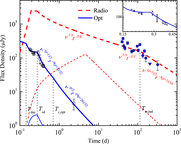
Figure 3: Fitting to the observed data. Solid lines correspond to optical light curves, and dashed lines to radio light curves, among which thick curves are for RS emission and thin curves for FS emission. Dotted vertical lines indicate the characteristic times. $T_{c,\mathrm{opt}}$ is the time $\nu_{c}=\nu_{\mathrm{opt}}$ whereafter the cooling frequency $\nu_{c}$ falls below the optical bandpass $\nu_{\mathrm{opt}}$, $T_{m,\mathrm{rad}}$ is the time $\nu_{m}=\nu_{\mathrm{rad}}$ whereafter the minimum frequency $\nu_{m}$ falls below the radio bandpass $\nu_{\mathrm{rad}}$. Inset is the zoom-in of the optical light curve. The data points are taken from Cenko et al. (2013).

References

- Abbott et al. (2009) Abbott, B.P. et al. 2009, RPPh, 72, 076901
- Acernese et al. (2008) Acernese, F. et al. 2008, CQGra, 25, 114045
- Atoyan (1999) Atoyan, A.M. 1999, A&A, 346, L49
- Barthelmy et al. (2005) Barthelmy, S.D. et al. 2005, Nature, 438, 994
- Berger (2007) Berger, E. 2007, ApJ, 670, 1254
- Berger et al. (2005) Berger, E. et al. 2005, Nature, 438, 988
- Blandford & McKee (1976) Blandford, R., & McKee, C. 1976, PhFl, 19, 1130
- Cenko et al. (2013) Cenko, S.B., Kulkarni, S.R., Horesh, A., Corsi, A., & Fox, D.B. 2013, ApJ, 769, 130
- Coroniti (1990) Coroniti, F.V. 1990, ApJ, 349, 538
- Dai (2004) Dai, Z.G. 2004, ApJ, 606, 1000
- Dai & Lu (1998a) Dai, Z.G., & Lu, T. 1998a, PhRvL, 81, 4301
- Dai & Lu (1998b) Dai, Z.G., & Lu, T. 1998b, A&A, 333, L87
- Dai et al. (2006) Dai, Z.G., Wang, X.Y., Wu, X.F., & Zhang, B. 2006, Science, 311, 1127
- Dermer et al. (2000) Dermer, C.D., Chiang, J., & Mitman, K.E. 2000, ApJ, 537, 785
- Duncan & Thompson (1992) Duncan, R.C., & Thompson, C. 1992, ApJL, 392, L9
- Eichler et al. (1989) Eichler, D., Livio, M., Piran, T., & Schramm, D. N. 1989, Nature, 340, 126
- Faber & Rasio (2012) Faber, J.A., & Rasio, F.A. 2012, LRR, 15, 8
- Fan & Xu (2006) Fan Y.-Z., & Xu, D. 2006, MNRAS, 372, L19
- Gao et al. (2013) Gao, H., Ding, X., Wu, X.F., Zhang, B., & Dai, Z.G. 2013, ApJ, 771, 86
- Gehrels et al. (2005) Gehrels, N. et al. 2005, Nature, 437, 851
- Giacomazzo & Perna (2013) Giacomazzo, B., & Perna, R. 2013, ApJL, 771, L26
- Hotokezaka et al. (2013) Hotokezaka, K. et al. 2013, PhRvD, 87, 024001
- Huang et al. (2002) Huang, Y.F., Dai, Z.G., & Lu, T. 2002, MNRAS, 332, 735
- Kluźniak & Ruderman (1998) Kluźniak, W., & Ruderman, M. 1998, ApJL, 505, L113
- Kulkarni (2005) Kulkarni, S. R. 2005, arXiv:astro-ph/0510256
- Kuroda et al. (2010) Kuroda, K., LCGT Collaboration 2010, CQGra, 27, 084004
- Lattimer (2012) Lattimer, J. M. 2012, ARNPS, 62, 485
- Li & Paczyński (1998) Li, L.-X., & Paczyński, B. 1998, ApJL, 507, L59
- Metzger & Berger (2012) Metzger, B.D., & Berger, E. 2012, ApJ, 746, 48
- Metzger et al. (2010) Metzger, B.D. et al. 2010, MNRAS, 406, 2650
- Michel (1994) Michel, F.C. 1994, ApJ, 431, 397
- Nakar & Piran (2011) Nakar, E., & Piran, T. 2011, Nature, 478, 82
- Palenzuela et al. (2013) Palenzuela, C. et al. 2013, arXiv:1301.7074
- Piran et al. (2013) Piran, T., Nakar, E., & Rosswog, S. 2013, MNRAS, 430, 2121
- Rezzolla et al. (2010) Rezzolla, L. et al. 2010, CQGra, 27, 114105
- Rezzolla et al. (2011) Rezzolla, L. et al. 2011, ApJL, 732, L6
- Rhoads (2003) Rhoads, J.E. 2003, ApJ, 591, 1097
- Roberts et al. (2011) Roberts, L. F., Kasen, D., Lee, W. H., & Ramirez-Ruiz, E. 2011, ApJL, 736, L21
- Rosswog (2005) Rosswog, S. 2005, ApJ, 634, 1202
- Rosswog et al. (2013) Rosswog, S., Piran, T., & Nakar, E. 2013, MNRAS, 430, 2585
- Rowlinson et al. (2010) Rowlinson, A. et al. 2010, MNRAS, 409, 531
- Rowlinson et al. (2013) Rowlinson, A. et al. 2013, MNRAS, 430, 1061
- Sari & Piran (1995) Sari, R., & Piran, T. 1995, ApJL, 455, L143
- Sari et al. (1998) Sari, R., Piran, T., & Narayan, R. 1998, ApJL, 497, L17
- Soderberg et al. (2006) Soderberg, A.M. et al. 2006, ApJ, 650, 261
- Thompson & Duncan (1993) Thompson, C., & Duncan, R.C. 1993, ApJ, 408, 194
- Wu et al. (2003) Wu, X.F., Dai, Z.G., Huang, Y.F., & Lu, T. 2003, MNRAS, 342, 1131
- Zhang (2013) Zhang, B. 2013, ApJL, 763, L22
- Zhang & Mészáros (2004) Zhang, B., & Mészáros, P. 2004, IJMPA, 19, 2385