GeV Emission during X-Ray Flares from Late Internal Shocks: Application to GRB 100728A

Abstract

Recently, the GeV radiation during the X-ray flare activity in GRB 100728A was detected by Feimi/LAT. Here we study the dynamics and emission properties of collision between two homogeneous shells based on the late internal shock model. The GeV photons can be produced from X-ray flare photons up-scattered by relativistic electrons accelerated by forward-reverse shocks, where involved radiative processes include synchrotron self-Compton and crossing inverse-Compton scattering. By analytical and numerical calculations, the observed spectral properties in GRB 100728A can be well explained.

1 Introduction

Gamma-ray bursts (GRBs) are the brightest explosive phenomena in the universe, the study of which has been being one of the most interesting fields in astrophysics. Thanks to the launch of the Fermi satellite in 2008, the Large Area Telescope (LAT) onboard Fermi has detected high-energy photons in energy range from 20 MeV to 300 GeV. Several mechanisms have been proposed to predict the origin of GeV photons along with the GRB afterglow phase (for a review see Zhang 2007): (1) In the external shock scenario, high-energy photons may be produced by synchrotron radiation and synchrotron self-Compton (SSC) processes from forward-reverse shocks (Meszaros & Rees & Papatheanassiou, 1994; Meszaros & Rees, 1994; Dermer et al., 2000; Zhang & Meszaros, 2001; Sari & Esin, 2001) or crossing inverse-Compton (CIC) processes between forward-reverse shocks (Wang et al., 2001a, b; Pe’er & Waxman, 2005). (2) In the hadronic and photo-pion scenario, there may be synchrotron radiation of protons, $\pi^{+}$ from $p\gamma$, $pn$ and $pp$ interactions, and positrons produced from $\pi^{+}$ decay and $\pi^{0}$ decay from $p\gamma$ interactions (Gupta & Zhang, 2007). (3) Electrons from pair productions during interaction of $>$100 GeV photons from GRBs with cosmic infrared background photons might also emit GeV photons by inverse scattering off cosmic microwave background photons (Dai & Lu, 2002; Wang et al., 2004).

On the other hand, one of the key discoveries is bright X-ray flares superimposing on underlying afterglow emission from nearly a half of GRBs observed by Swift (Burrows et al., 2005). The rapid rise and decay behavior of X-ray flares is widely understood as being due to some long-lasting activity of the central engines. Such an activity might be caused by an instable accretion disk around a black hole (Perna et al., 2006), accretion of fragments of the collapsing stellar core onto a central compact object in the collapsar model (King et al., 2005), a modulation of accretion flow by a magnetic barrier (Proga & Zhang, 2006), or magnetic reconnection of a newborn neutron star (Dai et al., 2006).

GRB 100728A is a case with simultaneous detections by Swift and Fermi (Abdo et al., 2011), which detected GeV photons during X-ray flares. The GeV photons during the X-ray flare activity detected by Fermi/LAT have been thought to arise from external inverse-Compton (EIC) scattering off X-ray flare photons by electrons in a relativistic forward shock (Fan & Piran, 2006; Fan et al., 2008; Wang et al., 2006; He et al., 2012). Here we propose a different explanation, in which the detected GeV photons are produced by SSC and CIC scattering off X-ray flare photons by electrons accelerated in the late internal shock model. This model was suggested by Fan & Wei (2005) and Zhang et al. (2006), and its motivations are based on two following facts. First, the rapid rising and decaying timescales and their distributions of X-ray flares require that the central engine restarts at a later time (Lazzati & Perna, 2007). Second, Liang et al. (2006) fitted the light curves of X-ray flares detected by Swift by assuming that the decaying phase of an X-ray flare is due to the high latitude emission from a relativistic outflow. These authors found that the ejection time of this outflow from the central engine is nearly equal to the peak time of an observed X-ray flare produced by the outflow.

This paper is organized as follows: we calculate the dynamics of a collision between two shells and properties of synchrotron and IC emission to produce X-ray flares and higher-energy emissions in section 2. In section 3, we present numerical calculations and light curves of the model. In this section, we also make an application to GRB 100728A and present constraints on the model parameters. In the final section, some conclusions are given.

2 The Synchrotron and IC Emission from Late Internal Shocks

In the internal shock model, a fireball consisting of a series of shells with different Lorentz factors can form prompt emission through shell-shell interactions. Similarly, collisions between shells with different velocities ejected from the central engine at late times after the GRB trigger can form late internal shocks, the emission from which reproduce X-ray flares.

2.1 Dynamics of Two Shell Collisions

For one X-ray flare we here consider the following shell-shell collision: a prior slow shell A with bulk lorentz factor $\gamma_{A}$ and kinetic-energy luminosity $L_{k,A}$, and a posterior fast shell B with bulk lorentz factor $\gamma_{B}$ $(\gamma_{A}<\gamma_{B})$ and kinetic-energy luminosity $L_{k,B}$. The collision of the two shells takes place at radius

$${R_{col}}={\beta_{B}}c\frac{{{\beta_{A}}\Delta{t_{ej}}}}{{({\beta_{B}}-{\beta_{A}})}}\simeq\frac{{2\gamma_{A}^{2}c\Delta{t_{ej}}}}{{1-{{({\gamma_{A}}/{\gamma_{B}})}^{2}}}}\equiv 2\gamma_{A}^{2}c\delta t,$$ (1)

where $\Delta{t_{ej}}$ is the ejection interval of the two shells, and $\delta t$ is redefined interval. During the collision, there are four regions separated by forward-reverse shocks: (1) the unshocked shell A, (2) the shocked shell A, (3) the shocked shell B, and (4) the shocked shell B, where regions 2 and 3 are separated by a contact discontinuity.

The particle number density of a shell measured in its comoving frame can be calculated by

$${n^{\prime}_{i}}=\frac{{{L_{k,i}}}}{{4\pi{R^{2}}\gamma_{i}^{2}{m_{p}}{c^{3}}}},$$ (2)

where $R$ is the radius of the shell and subscript $i$ can be taken as A or B.

Yu & Dai (2009) had analyzed the dynamics of a late-time shell-shell collision in detail. In order to get a high theoretical X-ray luminosity, it is reasonable to assume $\gamma_{A}\ll\gamma_{B}$ and $L_{k,A}=L_{k,B}\equiv L_{k}$. Assume that $\gamma_{1}$, $\gamma_{2}$, $\gamma_{3}$, and $\gamma_{4}$ are Lorentz factors of regions 1, 2, 3 and 4, respectively. As a result, we have $\gamma_{1}=\gamma_{A}$, $\gamma_{4}=\gamma_{B}$, and $n^{\prime}_{1}\gg n^{\prime}_{4}$. If a fast shell with low particle number density catches up with a slow shell with high particle number density and then collides with each other, a Newtonian forward shock (NFS) and a relativistic reverse shock (RRS) may be generated (Yu & Dai, 2009). So we can obtain $\gamma_{1}\simeq\gamma_{2}=\gamma_{3}=\gamma\ll\gamma_{4}$. Then, according to the jump conditions between the two sides of a shock (Blandford & McKee, 1976), the comoving internal energy densities of the two shocked regions can be calculated by ${e^{\prime}_{2}}=({\gamma_{21}}-1)(4{\gamma_{21}}+3){n^{\prime}_{1}}{m_{p}}{c^{2}},{e^{\prime}_{3}}=({\gamma_{34}}-1)(4{\gamma_{34}}+3){n^{\prime}_{4}}{m_{p}}{c^{2}}$, where $\gamma_{21}=\frac{1}{2}({\gamma_{1}}/{\gamma_{2}}+{\gamma_{2}}/{\gamma_{1}})$ and $\gamma_{34}=\frac{1}{2}({\gamma_{3}}/{\gamma_{4}}+{\gamma_{4}}/{\gamma_{3}})$ are the Lorentz factors of region 2 relative to the unshocked region 1, and region 3 relative to region 4, respectively. It is required that $e^{\prime}_{2}=e^{\prime}_{3}$ because of the mechanical equilibrium. We have

$$\frac{{({\gamma_{21}}-1)(4{\gamma_{21}}+3)}}{{({\gamma_{34}}-1)(4{\gamma_{34}}+3)}}=\frac{{n^{\prime}_{4}}}{{n^{\prime}_{1}}}={\left({\frac{{{\gamma_{1}}}}{{{\gamma_{4}}}}}\right)^{2}}\equiv f.$$ (3)

Two relative Lorentz factors can be calculated by ${\gamma_{21}}\approx\frac{{f\gamma_{4}^{2}}}{{7\gamma_{1}^{2}}}+1=\frac{8}{7}$, and ${\gamma_{34}}=\frac{{{\gamma_{4}}}}{{2{\gamma_{1}}}}\gg 1$. Assuming that $t$ is the observed shell interaction time since the X-ray flare onset, the radius of the system after the collision can be written as

$$R={R_{col}}+2{\gamma^{2}}ct\simeq 2{\gamma^{2}_{1}}c(t+\delta t).$$ (4)

During the propagation of the shocks and before the shock crossing, the total electron numbers in regions 2 and 3 can be calculated by ${N_{e,2}}=8\pi{R^{2}}{n^{\prime}_{1}}({\gamma_{21}}{\beta_{21}}/\gamma\beta){\gamma^{2}}ct$ and ${N_{e,3}}=8\pi{R^{2}}{n^{\prime}_{4}}({\gamma_{34}}{\beta_{34}}/\gamma\beta){\gamma^{2}}ct$ (Dai & Lu, 2002), respectively. We can easily find that the electron number in region 2 is larger than that in region 3.

2.2 Synchrotron Emission from Two Shocked Regions

As usual, we assume that fractions of $\epsilon_{B}$ and $\epsilon_{e}$ of the internal energy density in a GRB shock are converted into the energy densities of the magnetic field and electrons, respectively. Thus, using ${B^{\prime}_{i}}={(8\pi{\epsilon_{B}}{e^{\prime}_{i}})^{1/2}}$ for $i=$2 or 3, the strength of the magnetic field is calculated by

$${B^{\prime}_{2}}={B^{\prime}_{3}}={\left[\frac{{{\epsilon_{B}}L_{k}}}{{2{\gamma^{6}_{1}}{c^{3}}{{(t+\delta t)}^{2}}}}\right]^{1/2}}.$$ (5)

The electrons accelerated by the shocks are assumed to have a power-law energy distribution, $d{n^{\prime}_{e,i}}/d{\gamma^{\prime}_{e,i}}\propto{\gamma^{\prime}_{e}}^{-p}$ for ${\gamma^{\prime}_{e,i}}\geq{\gamma^{\prime}_{e,m,i}}$, where ${\gamma^{\prime}_{e,m,i}}$ is the minimum Lorentz factor. According to ${\gamma^{\prime}_{e,m,i}}=\frac{{{m_{p}}}}{{{m_{e}}}}(\frac{{p-2}}{{p-1}}){\epsilon_{e}}({\gamma_{\rm rel}}-1)$ (where ${\gamma_{\rm rel}}=\gamma_{21}$ or $\gamma_{34}$ in region 2 or 3), the minimum Lorentz factor can be written as

$$\begin{array}[]{c}{\gamma^{\prime}_{e,m,3}}\simeq 2.8\times{10^{3}}{g_{p}}{\epsilon_{e,-1/2}}{\gamma_{4,2.5}}\gamma_{1,1}^{-1},\end{array}$$ (6)

$$\begin{array}[]{c}{\gamma^{\prime}_{e,m,2}}\simeq 30{g_{p}}{\epsilon_{e,-1/2}},\end{array}$$ (7)

where $\epsilon_{e,-1/2}=\epsilon_{e}/10^{-1/2}$, $\gamma_{4,2.5}=\gamma_{4}/10^{2.5}$, $\gamma_{1,1}=\gamma_{1}/10^{1}$, and $g_{p}=3(p-2)/(p-1)$.

Moreover, the cooling Lorentz factor, above which the electrons lose most of their energies, ${\gamma^{\prime}_{e,c,i}}=6\pi{m_{e}}c/({y_{i}}{\sigma_{T}}{B^{\prime}_{3}}^{2}\gamma t)$, should be given by

$${\gamma^{\prime}_{e,c,3}}={\gamma^{\prime}_{e,c,2}}\simeq 1.4\times{10^{3}}y_{,0}^{-1}\varepsilon_{B,-3/2}^{-1}L_{k,50}^{-1}\gamma_{1,1}^{5}\frac{{(t+\delta t)_{,2}^{2}}}{{{t_{,-2}}}}.$$ (8)

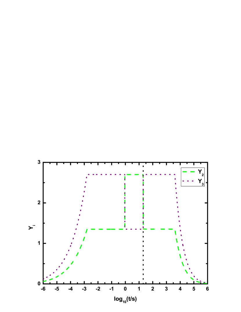
Figure 1: Ratio $Y_{i}$ of the IC to synchrotron luminosity as a function of time. The black dotted line represents the forward and reverse shock crossing time. Here we assume that the two shocks cross the two shells at a similar time $T_{crs}=20\,\mathrm{s}$. After the shock crossing time, the merged shell expands adiabatically if $s=3$ is assumed. The other parameters $L_{k,1}=L_{k,4}=10^{50}\mathrm{ergs^{-1}}$, $\gamma_{1}=10$, $\gamma_{4}=300$, $p=2.5$, $\epsilon_{e}=0.3$, $\epsilon_{B}=0.03$, $\theta_{jet}=0.1$, and $z=1$ are taken in numerical calculations.

where $y_{i}=1+Y_{i}$ is the ratio of the total luminosity to synchrotron luminosity, and $Y_{i}\approx[(4\eta_{i}\epsilon_{e}/\epsilon_{B}+1)^{1/2}-1]/2$ is the Compton parameter, which is defined by the ratio of the IC to synchrotron luminosity, with $\eta_{i}=\min[1,({\gamma^{\prime}_{e,c,i}}/{\gamma^{\prime}_{e,m,i}})^{2-p}]$ (Sari & Esin, 2001). Here we assume $\epsilon_{e}=0.3$ and $\epsilon_{B}=0.03$ in our calculations, so $y_{i}<3$ can be easily obtained so that we can assume $y_{i}\sim 1$. Fig. 1 presents changes of $Y_{i}$ and shows that it is reasonable to assume $y_{2}\sim y_{3}\sim 1$. Thus, the IC luminosity is comparable with the synchrotron luminosity.

In order to obtain the synchrotron emission spectrum, we consider

$${\nu_{m,i}}=\frac{{{q_{e}}}}{{2\pi{m_{e}}c}}{B^{\prime}_{i}}{\gamma^{\prime}}^{2}_{e,m,i}\gamma,$$ (9)

and

$${\nu_{c,i}}=\frac{{{q_{e}}}}{{2\pi{m_{e}}c}}{B^{\prime}_{i}}{\gamma^{\prime}}^{2}_{e,c,i}\gamma,$$ (10)

where $q_{e}$ is the electron charge. Four characteristic frequencies in regions 2 and 3,

$${\nu_{m,2}}\simeq 4.5\times{10^{13}}g_{p}^{2}\epsilon_{e,-1/2}^{2}\epsilon_{B,-3/2}^{1/2}L_{k,50}^{1/2}\gamma_{1,1}^{-2}(t+\delta t)_{,2}^{-1}\;\mathrm{Hz},$$ (11)

$${\nu_{m,3}}\simeq 5.0\times{10^{17}}g_{p}^{2}\epsilon_{e,-1/2}^{2}\epsilon_{B,-3/2}^{1/2}L_{k,50}^{1/2}\gamma_{4,2.5}^{2}\gamma_{1,1}^{-4}(t+\delta t)_{,2}^{-1}\;\mathrm{Hz},$$ (12)

and

$${\nu_{c,2}}={\nu_{c,3}}\simeq 1.3\times{10^{17}}y_{,0}^{-2}\epsilon_{B,-3/2}^{-3/2}L_{k,50}^{-3/2}\gamma_{1,1}^{8}\frac{{(t+\delta t)_{,2}^{3}}}{{t_{,-2}^{2}}}\;\mathrm{Hz},$$ (13)

can be obtained. In Fig. 2, their time evolutions are presented. From this figure, we can know easily that region 2 and region 3 are in the slow cooling regime at very early times, subsequently region 2 in the slow cooling regime but region 3 in the fast cooling regime, and finally both regions in the fast cooling regime. As a result, the spectral index between $\nu_{m}$ and $\nu_{c}$ of region 2 and region 3 has an evolution with time as Sari et al. (1998). It is reasonable that region 3 can be thought to be in the fast cooling regime, while region 2 is in the slow cooling regime at early times and in the fast cooling regime at later times. By applying the formula

$${F_{\nu,\max,i}}=\frac{{{N_{e,i}}}}{{4\pi D_{L}^{2}}}\frac{{{m_{e}}{c^{2}}{\sigma_{T}}}}{{3{q_{e}}}}{B^{\prime}_{i}}\gamma,$$ (14)

where $D_{L}$ is the luminosity distance of the burst, we obtain the peak flux density

$${F_{\nu,\max,2}}\simeq 0.11\epsilon_{B,-3/2}^{1/2}L_{k,50}^{3/2}\gamma_{1,1}^{-3}\frac{{{t_{,-2}}}}{{{{(t+\delta t)}_{,2}}}}D_{L,28}^{-2}\;\mathrm{Jy},$$ (15)

and

$${F_{\nu,\max,3}}\simeq 1.6\times{10^{-3}}\epsilon_{B,-3/2}^{1/2}L_{k,50}^{3/2}\gamma_{4,2.5}^{-1}\gamma_{1,1}^{-2}\frac{{{t_{,-2}}}}{{{{(t+\delta t)}_{,2}}}}D_{L,28}^{-2}\;\mathrm{Jy}.$$ (16)

According to equations (A1) and (A2) in appendix A (Sari et al., 1998), the synchrotron spectrum of region 2 in the slow cooling regime ($\nu_{m,2}<\nu_{c,2}$) is thus described by ${F_{\nu,2}}={F_{\nu,\max,2}}{(\nu/{\nu_{m,2}})^{-(p-1)/2}}$ for ${\nu_{m,2}}<\nu<{\nu_{c,2}}$ and ${F_{\nu,2}}={F_{\nu,\max,2}}{({\nu_{c,2}}/{\nu_{m,2}})^{-(p-1)/2}}{(\nu/{\nu_{c,2}})^{-p/2}}$ for $\nu>{\nu_{c,2}}$ or in the fast cooling regime ($\nu_{c,2}<\nu_{m,2}$) by ${F_{\nu,2}}={F_{\nu,\max,2}}{(\nu/{\nu_{c,2}})^{-1/2}}$ for ${\nu_{c,2}}<\nu<{\nu_{m,2}}$ and ${F_{\nu,2}}={F_{\nu,\max,2}}{({\nu_{m,2}}/{\nu_{c,2}})^{-1/2}}{(\nu/{\nu_{m,2}})^{-p/2}}$ for $\nu>{\nu_{m,2}}$. In the fast cooling regime of region 3, ${F_{\nu,3}}={F_{\nu,\max,3}}{(\nu/{\nu_{c,3}})^{-1/2}}$ for ${\nu_{c,3}}<\nu<{\nu_{m,3}}$ and ${F_{\nu,3}}={F_{\nu,\max,3}}{({\nu_{m,3}}/{\nu_{c,3}})^{-1/2}}{(\nu/{\nu_{m,3}})^{-p/2}}$ for $\nu>{\nu_{m,3}}$.

2.3 IC Emission from Two Shocked Regions

The ratio of IC to synchrotron emission luminosity $Y_{i}$ has been mentioned above (Fig. 1). Although regions 2 and 3 forming during the two-shell collision are optically thin to electron scattering, some synchrotron photons will be Compton scattered by shock-accelerated electrons, producing an additional IC component at higher-energy bands. Considering the highest energy electrons whose scattering enters the Klein-Nishina (KN) regime, the KN break frequency is calculated by

$$h\nu_{KN,3}^{SSC}=\frac{{{\gamma^{2}}m_{e}^{2}{c^{4}}}}{{h{\nu_{m,3}}}}\simeq 13g_{p}^{-2}\epsilon_{e,-1/2}^{-2}\epsilon_{B,-3/2}^{-1/2}L_{k,50}^{-1/2}\gamma_{4,2.5}^{-2}\gamma_{1,1}^{6}(t+\delta t)_{,2}\;\mathrm{GeV}.$$ (17)

Because of the characteristic frequency $h\nu_{m,3}\sim 1$ keV, and $\gamma^{\prime}_{e,m,3}\sim 10^{3}$, we can obtain $(\gamma^{\prime}_{e,m,3}h\nu_{m,3})/(m_{e}c^{2})\sim 1$. So in the analysis estimates, it is reasonable to use the Thomson optical depth of the electrons in regions 2 and 3, which can be calculated by ${\tau_{i}}=\frac{{{\sigma_{T}}{N_{e,i}}}}{{4\pi{R^{2}}}}$, where $i=2$ or $3$. We calculate the upscattered spectral characteristic frequencies of IC process, as in Sari & Esin (2001). Region 3 is in the fast cooling regime and its SSC break frequencies become

$$h\nu_{m,3}^{ssc}=2{\gamma^{\prime}}^{2}_{e,m,3}h{\nu_{m,3}}\simeq 32g_{p}^{4}\epsilon_{e,-1/2}^{4}\epsilon_{B,-3/2}^{1/2}L_{k,50}^{1/2}\gamma_{4,2.5}^{4}\gamma_{1,1}^{-6}(t+\delta t)_{,2}^{-1}\;\mathrm{GeV},$$ (18)

and

$$h\nu_{c,3}^{ssc}=2{\gamma^{\prime}}^{2}_{e,c,3}h{\nu_{c,3}}\simeq 2.1y_{,0}^{-4}\epsilon_{B,-3/2}^{-7/2}L_{k,50}^{-7/2}\gamma_{1,1}^{18}\frac{{(t+\delta t)_{,2}^{7}}}{{t_{,-2}^{4}}}\;\mathrm{GeV}.$$ (19)

Obviously, the SSC peak energy for region 3 is in the KN regime and $h\nu_{m,3}^{ssc}$ is comparable with $h\nu_{KN,3}^{SSC}$. As Tavecchio et al. (1998) suggested, no matter whether the SSC peak frequency enters the KN regime or not, the spectral index of SSC emission at low energy band has the same power-law approximation as synchrotron emission. So the SSC flux of the fast-cooling region 3, ${F_{\nu,3}^{SSC}}={F_{\nu,\max,3}^{SSC}}{(\nu/{\nu_{c,3}^{SSC}})^{-1/2}}$ for ${\nu_{c,3}^{SSC}}<\nu<\nu_{cri}$, where $\nu_{cri}\sim\min({\nu_{m,3}^{SSC}}$, ${\nu_{KN,3}^{SSC}}$). As a result, the peak flux at $\nu_{KN,3}^{SSC}$ is

$$[\nu{F_{\nu}}]_{p,3}^{SSC} = \nu_{KN,3}^{SSC}{\tau_{3}}{F_{\nu,\max,3}}{\left(\frac{{\nu_{KN,3}^{SSC}}}{{\nu_{c,3}^{ssc}}}\right)^{-1/2}}$$ (20)

$$\simeq 6.7\times{10^{-9}}g_{p}^{-1}y_{,0}^{-2}\epsilon_{e,-1/2}^{-1}\epsilon_{B,-3/2}^{-3/2}L_{k,50}^{1/2}\gamma_{4,2.5}^{-3}\gamma_{1,1}^{6}(t+\delta t)_{,2}D^{-2}_{L,28}\;\mathrm{erg\,cm^{-2}s^{-1}}.$$

Region 2 is in the slow cooling regime, its SSC break frequencies are $\nu_{m,2}^{SSC}=2{\gamma^{\prime}}^{2}_{e,m,2}{\nu_{m,2}}\simeq 8.1\times{10^{16}}g_{p}^{4}\epsilon_{e,-1/2}^{4}\epsilon_{B,-3/2}^{1/2}L_{k,50}^{1/2}\gamma_{1,1}^{-2}{(t+\delta t)^{-1}}\;\mathrm{Hz}$ and $\nu_{c,2}^{ssc}=\nu_{c,3}^{ssc}$. Thus we can obtain a very low peak flux

$$[\nu{F_{\nu}}]_{p,2}^{SSC} = \nu_{c,2}^{SSC}{\tau_{2}}{F_{\nu,\max,2}}{\left(\frac{{\nu_{c,2}^{SSC}}}{{\nu_{m,2}^{SSC}}}\right)^{-(p-1)/2}}$$ (21)

$$\simeq 9.8\times{10^{-11}}y_{,0}^{-1}g_{p}^{3}\epsilon_{e,-1/2}^{3}L_{k,50}^{2}\gamma_{1,1}^{-5}\frac{{t_{,-2}}}{{(t+\delta t)_{,2}^{2}}}D^{-2}_{L,28}\;\mathrm{erg\,cm^{-2}s^{-1}},$$

where $p=2.5$ is assumed. Obviously, the SSC radiation of region 2 is much weaker than that of region 3.

Apart from the SSC scattering processes in regions 2 and 3, the two other cross-IC scattering processes are also presented. Assuming the thin shell approximation, about one-half of the photons produced in one shocked region will diffuse into the other one in the comoving frame. We can obtain the low and high characteristic frequencies in the following cases.
(1) The synchrotron photons in region 2 are scattered by electrons in region 3,

$$\nu_{L,3}^{CIC} = 2{\gamma^{\prime}}^{2}_{e,c,3}{\nu_{m,2}}$$ (22)

$$\simeq 1.76\times{10^{20}}y_{,0}^{-2}g_{p}^{2}\epsilon_{e,-1/2}^{2}\epsilon_{B.-3/2}^{-3/2}{L^{-3/2}}\gamma_{1,1}^{8}\frac{{(t+\delta t)_{,2}^{3}}}{{t_{,-2}^{2}}}\;\mathrm{Hz},$$

$$\nu_{H,3}^{CIC} = 2{\gamma^{\prime}}^{2}_{e,m,3}{\nu_{c,2}}$$ (23)

$$\simeq 1.97\times{10^{24}}y_{,0}^{-2}g_{p}^{2}\epsilon_{e,-1/2}^{2}\epsilon_{B.-3/2}^{-3/2}{L^{-3/2}}\gamma_{4,2.5}^{2}\gamma_{1,1}^{6}\frac{{(t+\delta t)_{,2}^{3}}}{{t_{,-2}^{2}}}\;\mathrm{Hz},$$

and the peak flux at $\nu_{H,3}^{CIC}$ can be estimated to be $[\nu{F_{\nu}}]_{p,3}^{CIC}\sim 1\times{10^{-9}}\mathrm{erg\,cm^{-2}s^{-1}}$.
(2) The synchrotron photons in region 3 are scattered by electrons in region 2,

$$\nu_{L,2}^{CIC} = 2{\gamma^{\prime}}^{2}_{e,m,2}{\nu_{c,3}}$$ (24)

$$\simeq 2.34\times{10^{20}}y_{,0}^{-2}g_{p}^{2}\epsilon_{e,-1/2}^{2}\epsilon_{B.-3/2}^{-3/2}{L^{-3/2}}\gamma_{1,1}^{8}\frac{{(t+\delta t)_{,2}^{3}}}{{t_{,-2}^{2}}}\;\mathrm{Hz},$$

$$\nu_{H,2}^{CIC} = 2{\gamma^{\prime}}^{2}_{e,c,2}{\nu_{m,3}}$$ (25)

$$\simeq 1.96\times{10^{24}}y_{,0}^{-2}g_{p}^{2}\epsilon_{e,-1/2}^{2}\epsilon_{B.-3/2}^{-3/2}{L^{-3/2}}\gamma_{4,2.5}^{2}\gamma_{1,1}^{6}\frac{{(t+\delta t)_{,2}^{3}}}{{t_{,-2}^{2}}}\;\mathrm{Hz},$$

and the peak flux at $\nu_{H,2}^{CIC}$ can be estimated to be $[\nu{F_{\nu}}]_{p,2}^{CIC}\sim 1\times{10^{-9}}\mathrm{erg\,cm^{-2}s^{-1}}$.

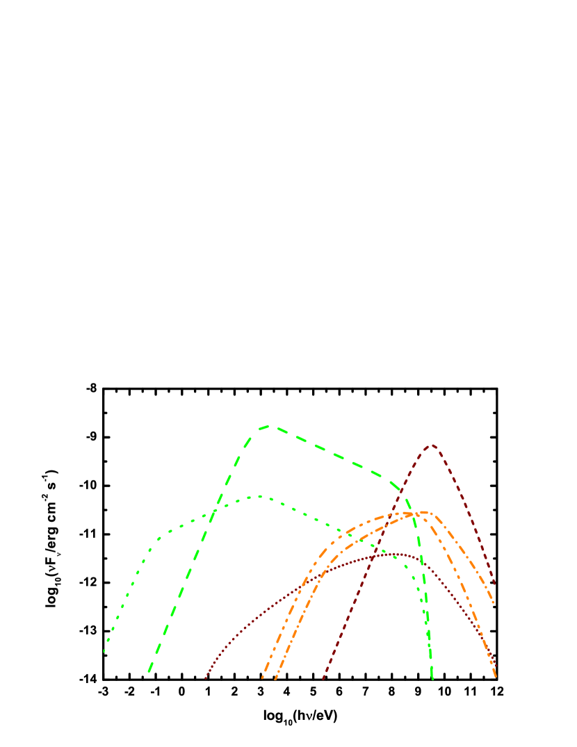
Figure 3: Time-resolved spectra of the six components at $t=10$ ms. The green dotted line and dashed line represent the synchrotron emission of regions 2 and 3, respectively. The wine short-dotted line and short-dashed line represent the SSC emission of regions 2 and 3, respectively. The orange dash-dot-dotted line and short-dash-dotted line represent the CIC emission, respectively. The same parameters as in Fig. 1 are taken in numerical calculations.

From the above equations and Fig. 3, for synchrotron emission, region 3 is more important than region 2. For IC emission, we can also see that the SSC emission of region 3 is the most important among the IC components, while the SSC emission of region 2 is the weakest. This is very easy to understand, since the electrons in region 3 have larger Lorentz factors due to RRS but the electrons in region 2 have smaller Lorentz factors due to NFS.

3 Application to GRB 100728A and Numerical Calculations

3.1 Parameter Limits

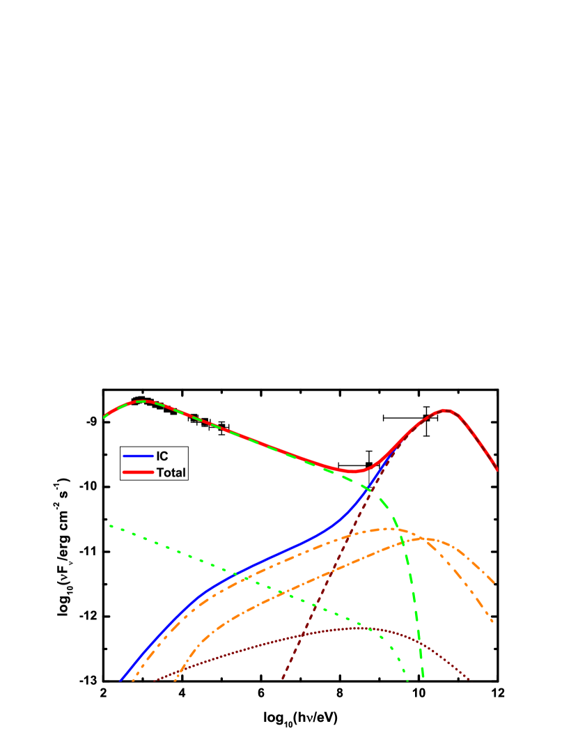
Figure 4: Time-averaged spectra of the X-ray and GeV emission of GRB 100728A and fitting this burst with our model. The observed data are taken from Abdo et al. (2011), which are fitted by a time-averaged spectrum from $t=0\,\mathrm{s}$ to $t=10^{1.8}\,\mathrm{s}$. The green dotted line and dashed line represent the synchrotron emission of regions 2 and 3, respectively. The wine short-dotted line and short-dashed line represent the SSC emission of regions 2 and 3, respectively. The orange dash-dot-dotted line and short-dash-dotted line represent the CIC emission, respectively. The blue thin solid line represents the total IC including SSC and CIC and the red thick solid line represents the sum of synchrotron and IC emission. The other parameters $L_{k,1}=7.0\times 10^{50}\mathrm{ergs^{-1}}$, $L_{k,4}=2.5\times 10^{50}\mathrm{ergs^{-1}}$, $\gamma_{1}=50$, $\gamma_{4}=5830$, $p=2.48$, $\epsilon_{e}=0.3$, $\epsilon_{B}=0.03$, $\theta_{jet}=0.1$, and $z=1$ are taken in numerical calculations.

The Fermi/GBM triggered GRB 100728A at 02:17:31 UT, 53.6 s before the Swift/BAT trigger. The duration of this burst is $T_{90}\sim 163$ s. Several apparent X-ray flares were observed by Swift/XRT, while significant GeV photons were detected by Fermi/LAT during the early afterglow phase. We can obtain the observed properties of this GRB: 1) From XRT, the time-averaged spectrum of these flares from $t\sim 167$ s to $854$ s can be fitted well by the Band function (Band et al., 1993) with the low energy slope of $\alpha=-1.06\pm 0.11$, the high energy slope $\beta=-2.24\pm 0.02$ and the peak energy $E_{pk}=1.0_{-0.4}^{+0.8}\,\mathrm{keV}$ (Abdo et al., 2011). 2) From LAT, the spectrum of the GeV emission is fitted well with photon index of $\Gamma_{LAT}=-1.4\pm 0.2\,\,(1\sigma)$ (Abdo et al., 2011) and the flux $F_{LAT}\sim(5.8\pm 4.5)\times 10^{-9}\,\mathrm{erg\,cm^{-2}s^{-1}}$ (He et al., 2012) during the period of $t\sim 167$ s to $854$ s. We use our model with reasonable parameters to fit the GRB100728A time-averaged energy spectrum (Fig. 4). The data points in this figure are taken from Abdo et al. (2011), from $T_{0}+254\,\mathrm{s}$ to $T_{0}+854\,\mathrm{s}$ about $7$ flares, where $T_{0}$ is the trigger time. The duration of one flare is about tens of seconds. Taking into account the similarity among the flares generated, we only model one flare induced by a collision between two shells to fit the interval data, so we choose the time from the onset of two-shell interaction, i.e., $t=0\,\mathrm{s}$ to $t=10^{1.8}\,\mathrm{s}$, where the latter time is comparable with the duration of one flare of GRB 100728A.

The emission of region 3 is the most important, and is used to explain the observations on GRB100728A. Since region 3 is in the fast cooling regime and the high energy slope $\beta=-2.24\pm 0.02$, we can obtain the electron distribution index $p=2.48\pm 0.04$. For ${\nu_{c,3}}<\nu<{\nu_{m,3}}$ and ${\nu_{c,3}^{SSC}}<\nu<{\nu_{cri}}$, the synchrotron spectrum and SSC component of an X-ray flare have the same photon index of $-3/2$, which is consistent with the observed GeV emission, $\Gamma_{LAT}=-1.4\pm 0.2$. The low energy slope of $\alpha=-1.06\pm 0.11$, which may be caused by the low frequency absorption effect, can also be regarded as a consistent result within the acceptable range.

In the two-shell collision model, we only regard the kinetic-energy luminosity $L_{k}$, Lorentz factors $\gamma_{1}$ and $\gamma_{4}$ as variable parameters. Because of $h\nu_{m,3}\sim E_{pk}=1.0_{-0.4}^{+0.8}\,\mathrm{keV}$ and $h\nu_{m,3}^{SSC}\gtrsim h\nu_{KN,3}^{SSC}\sim h\nu_{pk}^{LAT}>10\,$GeV, from the ratio of equations (12) and (18), $\gamma_{4}/\gamma_{1}>30$ is required, which is consistent with the dynamical analysis. This suggests that the posterior shell can catch up with the prior shell very soon and an NFS and a RRS can be formed. Furthermore, according to equation (20) and $F_{LAT}\sim(5.8\pm 4.5)\times 10^{-9}\,\mathrm{erg\,cm^{-2}s^{-1}}$, we obtain $L_{k}\sim 0.9\pm 0.8\times 10^{50}\,\mathrm{erg\,cm^{-2}s^{-1}}$. Finally, for equation (12) and $h\nu_{m,3}\sim E_{pk}=1.0_{-0.4}^{+0.8}\,\mathrm{keV}$, we can obtain $\gamma_{4}/\gamma_{1}^{2}\sim\mathrm{few}$, which is an essential condition to produce a bright X-ray flare.

In addition, the optical depth due to pair production can be given by (Lithwick & Sari, 2001)

$${\tau_{\gamma\gamma}}=\frac{{(11/180){\sigma_{T}}{N_{>{\nu_{m,an}}}}}}{{4\pi R^{2}}},$$ (26)

where ${N_{>{\nu_{m,an}}}}$ is the photon number with frequency up to ${\nu_{m,an}}$ with $h\nu_{m,an}\equiv(\gamma m_{e}c^{2})^{2}/h{\nu_{m}}$, which can annihilate the ${\nu_{m}}\sim 1\,\mathrm{keV}$ photons. So ${N_{>{\nu_{m,an}}}}\simeq L_{GeV}t/(h{\nu_{m,an}})$ can be used to estimate the photon number with frequency up to ${\nu_{m,an}}$, where $L_{GeV}$ is the GeV luminosity. Besides, $R=2\gamma^{2}c\delta t\sim 2\times 10^{14}\,\mathrm{cm}$, so we can get

$${\tau_{\gamma\gamma}}\sim 2\times{10^{-3}}L_{GeV,50}\gamma_{,1}^{-6}\delta{t^{-2}_{,2}}{t_{,1}},$$ (27)

which indicates that the pair production effect is unimportant. As a result, the secondary electrons produced by the pair production effect is ignored here.

To summarize, the GeV emission of GRB100728A can be described well by the IC process of the electrons accelerated by forward-reverse shocks in regions 2 and 3. Using reasonable and appropriate values of the model parameters, we present good fitting results (Fig. 4).

3.2 Numerical Calculations of the Model

The results mentioned above are analytical estimates, while all the figures except for Figures 1 and 2 in this paper are based on more detailed and precise numerical calculations. Next we will describe numerical methods.

As mentioned above, the electrons accelerated by the shocks are assumed to have a power-law energy distribution, $d{n^{\prime}_{e}}/d{\gamma^{\prime}_{e}}\propto{\gamma^{\prime}_{e}}^{-p}$ for ${\gamma^{\prime}_{e}}\geq{\gamma^{\prime}_{e,m}}$, where ${\gamma^{\prime}_{e,m}}$ is the minimum Lorentz factor. When the electron cooling effect is considered, the resulting electron distribution in the comoving frame takes the following forms:
(1) If the newly shocked electrons cool faster than the shock dynamical timescale, i.e. fast cooling ($\gamma^{\prime}_{e,m}>\gamma^{\prime}_{e,c}$),

$$\frac{{d{n^{\prime}_{e}}}}{{d{\gamma^{\prime}_{e}}}}\propto\left\{\begin{array}[]{ll}{\gamma^{\prime}_{e}}^{-2}&{\gamma^{\prime}_{e,c}}<{\gamma^{\prime}_{e}}<{\gamma^{\prime}_{e,m}}\\ {\gamma^{\prime}_{e}}^{-p-1}&{\gamma^{\prime}_{e,m}}<{\gamma^{\prime}_{e}}<{\gamma^{\prime}_{e,\max}};\end{array}\right.$$ (28)

(2) If the newly shocked electrons cool slower than the shock dynamical timescale, i.e. slow cooling ($\gamma^{\prime}_{e,m}<\gamma^{\prime}_{e,c}$),

$$\frac{{d{n^{\prime}_{e}}}}{{d{\gamma^{\prime}_{e}}}}\propto\left\{\begin{array}[]{ll}{\gamma^{\prime}_{e}}^{-p}&{\gamma^{\prime}_{e,m}}<{\gamma^{\prime}_{e}}<{\gamma^{\prime}_{e,c}}\\ {\gamma^{\prime}_{e}}^{-p-1}&{\gamma^{\prime}_{e,c}}<{\gamma^{\prime}_{e}}<{\gamma^{\prime}_{e,\max}},\end{array}\right.$$ (29)

where ${\gamma^{\prime}_{e,\max}}$ is the maximum Lorentz factor of shocked electrons in the comoving frame, which is determined by equating the electron acceleration timescale with the timescale of the non-thermal emission (including synchrotron and IC emission) cooling timescale.

From the electron distribution, the synchrotron seed photon spectrum can be obtained easily (Rybicki & Lightman, 1979). After we obtain the electron distribution and the seed photon spectrum, the emission of seed synchrotron photons up-scattered by relativistic electrons accelerated by forward-reverse shocks can be computed. For simplicity, we only consider the first-order IC and neglect higher order IC processes. In the Thomson regime, therefore, the IC volume emissivity in the comoving frame can be given by (Rybicki & Lightman, 1979; Sari & Esin, 2001)

$${j^{\prime}}_{\nu}^{IC}=3{\sigma_{T}}\int_{{\gamma^{\prime}_{e,m}}}^{\gamma^{\prime}_{e,max}}{d{\gamma^{\prime}_{e}}}\frac{{d{n^{\prime}_{e}}}}{{d{\gamma^{\prime}_{e}}}}\int_{0}^{1}{dxg(x){{\tilde{f}^{\prime}}_{{{\nu^{\prime}}_{s}}}}(x)},$$ (30)

where $x=\nu^{\prime}/(4{{\gamma^{\prime}}_{e}^{2}}\nu^{\prime}_{s})$ , $\nu^{\prime}_{s}$ is the synchrotron seed photon frequency in the comoving frame, ${{\tilde{f}^{\prime}}_{{{\nu^{\prime}}_{s}}}}(x)$ is the incident-specific flux at the shock front in the comoving frame, and $g(x)=1+x+2x\ln x-2x^{2}$ considers the angular dependence of the scattering cross section in the limit $\gamma^{\prime}_{e}\gg 1$ (Blumenthal & Gould, 1970; Sari & Esin, 2001). We can convert the comoving-frame quantities to observed quantities, by considering ${f^{\prime}}_{\nu}^{IC}={j^{\prime}}_{\nu}^{IC}4\pi{R^{2}}\Delta R^{\prime}/4\pi{D^{2}}$ and ${{f^{\prime}}_{\nu^{\prime}}}={{\tilde{f}^{\prime}}_{{{\nu^{\prime}}_{s}}}}4\pi{R^{2}}/4\pi{D^{2}}$, where $R$ is the shock radius, $D$ is the distance to the observer, $\Delta R^{\prime}$ is the comoving width of the shocked shell (Sari & Esin, 2001; Wang et al., 2001b). So we obtain the IC flux in the observer frame,

$$f_{\nu}^{IC}=3\Delta R^{\prime}{\sigma_{T}}\int_{{{\gamma^{\prime}}_{e,m}}}^{{{\gamma^{\prime}}_{e,\max}}}{d{{\gamma^{\prime}}_{e}}}\frac{{d{{n^{\prime}}_{e}}}}{{d{{\gamma^{\prime}}_{e}}}}\int_{0}^{1}{dxg(x){f_{\nu}}(x)}.$$ (31)

If ${\gamma^{\prime}_{e}}h{\nu^{\prime}_{s}}\gtrsim{m_{e}}c^{2}$, the Klein-Nishina regime should be considered. Equation (30) can be replaced by (Blumenthal & Gould, 1970)

$${j^{\prime}}_{\nu}^{IC}=3{\sigma_{T}}\int_{{{\gamma^{\prime}}_{e,m}}}^{{{\gamma^{\prime}}_{e,\max}}}{d{{\gamma^{\prime}}_{e}}}\frac{{d{{n^{\prime}}_{e}}}}{{d{{\gamma^{\prime}}_{e}}}}\int_{{{\nu^{\prime}}_{s,\min}}}^{\infty}{d{{\nu^{\prime}}_{s}}\frac{{\nu^{\prime}{{\tilde{f}^{\prime}}_{{{\nu^{\prime}}_{s}}}}}}{{4{\gamma^{2}}{\nu^{\prime}}_{s}^{2}}}[1+x+2x\ln x-2{x^{2}}+\frac{1}{2}\frac{{{x^{2}}{y^{2}}}}{{1+xy}}(1-x)]},$$ (32)

where $y=4{\gamma^{\prime}_{e}}h\nu^{\prime}_{s}/(m_{e}c^{2})$ and $x=h\nu^{\prime}/[y({\gamma^{\prime}_{e}}m_{e}c^{2}-h\nu^{\prime})]=\nu^{\prime}/(4{{\gamma^{\prime}}_{e}^{2}}\nu^{\prime}_{s}-y\nu^{\prime})$.

3.3 Light Curves of the Model

We now calculate synchrotron and IC emission light curves. It can be predicted that both emissions will have a good temporal coincidence, because they are produced from the same region. This may be the most important difference from the EIC model, because in the latter model the GeV emission will last for a period much longer than the duration of the GeV emission based on the curvature effect of an external forward shock and is mainly extended by the highly anisotropic radiation of the upscattered photons.

Yu & Dai (2009) presented the theoretical X-ray flare light curves produced by considering a collision of two homogeneous shells. Here we give both X-ray and GeV emission light curves based on more precise numerical calculations in our assumed dynamics in Fig. 5. A basic characteristic of the X-ray flare is that its light curve has a rapid rise and fall. The rapid rise can be clearly seen by resetting the time zero point in the right panel of Fig. 5. Before the two shocks’ crossing time $T_{crs}$, by ignoring possible spreading of the hot shocked materials, evolutions of $\nu_{c,i}$, $\nu_{m,i}$, and $F_{\nu,max,i}$ follow equations (11), (12), (13), (15), and (16). After $T_{crs}$, the spreading of the hot materials into the vacuum cannot be ignored and the merged shell experiences an adiabatic cooling. During this phase, a simple power-law of the volume of the merged shell is assumed as $V^{\prime}_{i}\propto R^{s}$, where $s$ is a free parameter and its value is taken to be from 2 to 3. As a result, the particle number densities would decrease as $n^{\prime}_{i}\propto{V^{\prime}}_{i}^{-1}\propto R^{-s}$, the internal energy densities as $e^{\prime}_{i}\propto{V^{\prime}}_{i}^{-4/3}\propto R^{-4s/3}$, and the magnetic field strength as $B^{\prime}_{i}\propto(e^{\prime}_{i})^{-1/2}\propto R^{-2s/3}$. From equation (4), before $\delta t$, any increase of the radius $R$ can be ignored (i.e., $R\simeq{\rm constant}$), but after $\delta t$, the radius increases linearly with time (i.e., $R\propto t$). For simplicity, we consider $T_{crs}\simeq\delta t$. So the characteristic quantities can be presented by

$${\nu_{m}}\propto\left\{\begin{array}[]{ll}{t^{0}}&t<{T_{crs}}\\ {t^{-2s/3}}&t>{T_{crs}},\end{array}\right.$$ (33)

$${\nu_{c}}\propto\left\{\begin{array}[]{ll}{t^{-2}}&t<{T_{crs}}\\ {t^{2s-2}}&t>{T_{crs}},\end{array}\right.$$ (34)

and

$${F_{\nu,\max}}\propto\left\{\begin{array}[]{ll}t&t<{T_{crs}}\\ {t^{-2s/3}}&t>{T_{crs}}.\end{array}\right.$$ (35)

For clarity, the subscript $i$ is omitted. The theoretical light curve of an X-ray flare has been given in appendix A.

The intrinsic decline slope of the last segment of the theoretical light curves is $\alpha=(sp+s)/3$ (where $\alpha=-d\log F_{\nu}/d\log t$). Liang et al. (2006) found that the rapid decline of most X-ray flares seems to be consistent with the curvature effect by fitting the light curves of X-ray flares detected by Swift and that the temporal index is equal to the simultaneous spectral index plus $2$. In the last segment of the theoretical light curves, the corresponding spectral index is $(p-1)/2$ for $\nu_{m}<\nu_{X_{band}}<\nu_{c}$, where $\nu_{X_{band}}\sim 10^{17}\mathrm{Hz}$. For $s=3$ and $2<p<3$, we find

$$\alpha=\frac{{3p+3}}{3}>\frac{{p-1}}{2}+2.$$ (36)

So the X-ray flux would have a rapid decline owing to the curvature effect.

Similarly, in the left panel of Fig. 5, several apparent power-law forms are written as

$${F_{\nu}}\propto\left\{\begin{array}[]{ll}t&t<{T_{cm}}\\ {t^{0}}&{T_{cm}}<t<{T_{crs}}\\ {t^{\frac{{s-3}}{3}}}&{T_{crs}}<t<{T_{m}}\\ {t^{-\frac{{sp-2s+3}}{3}}}&t>{T_{m}}.\end{array}\right.$$ (37)

The temporal index $\alpha$ of the last segment of the light curves is $(sp-2s+3)/3$. Although this temporal index cannot easily satisfy equation (36), it cannot be ruled out absolutely. This is because the segment near the flare onset time may be steepened by the time zero effect dramatically. This effect can be seen by comparing the right panel with the left panel of Fig. 5, where the right panel resets the time zero point, having a larger slope. So X-ray flares formed by two-shell interactions are characteristic of a rapid rise and fall.

In Fig. 5, the X-ray and GeV emission have a similar evolution with time, which can be easily seen in the right panel. It is this behavior that we want to specify both time coincidence.

4 Conclusions

In this paper, the late internal shock origin for X-ray flares is adopted, and a collision of two homogeneous shells is analyzed in quantitative calculations. Besides this model, X-ray flares may be produced by a delayed external shock (Piro et al., 2005; Galli & Piro, 2007). Both models suggest a prolonged central engine activity. Wu et al. (2005) made a quantitative analysis in two cases, and suggested that two kinds of X-ray flares are not excluded, and even maybe coexist for a certain GRB.

The strong SSC and CIC emission during X-ray flares had been analyzed and found to be detectable with high energy telescopes (Fan et al., 2008; Yu & Dai, 2009). GRB 100728A is the second case (after GRB090510) to date with simultaneous Swift and Fermi observations, in which the GeV and X-ray emission maybe have the same origin because of the temporal coincidence. Thus, the afterglow synchrotron and SSC emission scenarios may be slightly far-fetched. It is natural that high energy emission can be generated during X-ray flares by inverse Compton processes. He et al. (2012) provided an explanation for GRB 100728A in the EIC scenario, in which X-ray flare photons are up-scattered by electrons in an external forward shock. We here give an alternative reasonable explanation by using the SSC and CIC scenario where X-ray flare photons are up-scattered by electrons accelerated by forward-reverse shocks in the late internal shock model. One main difference between the two scenarios is whether there is a good temporal correlation between X-ray and GeV emission (Fan et al., 2008). In the SSC and CIC scenario, a good temporal correlation between X-ray and GeV emission is expected (Fig. 5), whereas GeV photons in the EIC scenario maybe have a significant temporal extension and even last a time much longer than the duration of one X-ray flare (Fan et al., 2008). So, no obvious temporal extension of GeV photons for GRB 100728A supports the SSC and CIC scenario. In fact, both the SSC and CIC scenario and the EIC scenario are not excluded and maybe coexist in high energy emission, because the extended GeV emission flux in the EIC scenario may be too weak (compared with that in the SSC and CIC scenario) to be detected.

Appendix A Appendix

Here we present the theoretical X-ray flare light curves in the parameters of Fig. 2. The synchrotron energy spectrum can obtained from Sari et al. (1998).
(1) In the fast cooling regime, the energy spectrum is discribed by

$${F_{\nu}}=\left\{\begin{array}[]{ll}{(\nu/{\nu_{c}})^{1/3}}{F_{\nu,\max}}&\nu<{\nu_{c}}\\ {(\nu/{\nu_{c}})^{-1/2}}{F_{\nu,\max}}&{\nu_{c}}<\nu<{\nu_{m}}\\ {(\nu/{\nu_{m}})^{-p/2}}{({\nu_{m}}/{\nu_{c}})^{-1/2}}{F_{\nu,\max}}&{\nu_{m}}<\nu;\end{array}\right.$$ (A1)

(2) And for slow cooling, the energy spectrum reads

$${F_{\nu}}=\left\{\begin{array}[]{ll}{(\nu/{\nu_{m}})^{1/3}}{F_{\nu,\max}}&\nu<{\nu_{m}}\\ {(\nu/{\nu_{m}})^{-(p-1)/2}}{F_{\nu,\max}}&{\nu_{m}}<\nu<{\nu_{c}}\\ {(\nu/{\nu_{c}})^{-p/2}}{({\nu_{c}}/{\nu_{m}})^{-(p-1)/2}}{F_{\nu,\max}}&{\nu_{c}}<\nu.\end{array}\right.$$ (A2)

For a specific x-ray band in Fig. 2, from equations and equations (33), (34), and (35), the theoretical X-ray flare light curves can be given by

$${F_{\nu}}\propto\left\{\begin{array}[]{ll}t&t<{T_{cm1}}\\ {t^{5/3}}&{T_{cm1}}<t<{T_{c1}}\\ {t^{0}}&{T_{c1}}<t<{T_{crs}}\\ {t^{\frac{{s-3}}{3}}}&{T_{crs}}<t<{T_{m}}\\ {t^{-\frac{{sp-2s+3}}{3}}}&{T_{m}}<t<{T_{cm2}}\\ {t^{-\frac{{sp-2s+3}}{3}}}&{T_{cm2}}<t<{T_{c2}}\\ {t^{-\frac{{sp+s}}{3}}}&t>{T_{c2}}.\end{array}\right.$$ (A3)

where $T_{cm1}(T_{cm2})$ is the first (second) time $\nu_{c}=\nu_{m}$, and $T_{m}$($T_{c1}$ or $T_{c2}$, $T_{c1}$ for the first time and $T_{c2}$ for the second time) is the time of the break frequency $\nu_{m}$($\nu_{c}$) passing through the X-ray band (about $10^{17}\,\mathrm{Hz}$) in region 3. It should be pointed out that there may be a mistake in Yu & Dai (2009), which gave a temporal index $(sp+3)/3$ for $t>{T_{c2}}$.

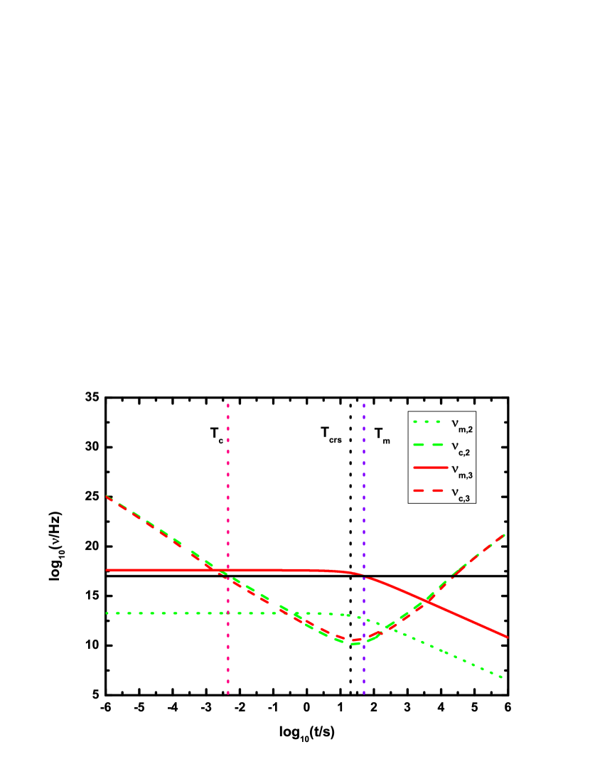
Figure 2: Four characteristic frequencies as functions of time. The black vertical dotted line represents the forward and reverse shock crossing time. A similar crossing time $T_{crs}=20\,\mathrm{s}$ of two shocks is also assumed. After the shock crossing time, the merged shell expands adiabatically if $s=3$ is assumed. $T_{m}$($T_{c}$) is the time of the break frequency $\nu_{m}$($\nu_{c}$) passing through the X-ray band (black horizontal solid line, $~{}10^{17}\,\mathrm{Hz}$) in the region 3 (Yu & Dai, 2009). The same parameters as in Fig. 1 are taken in numerical calculations.

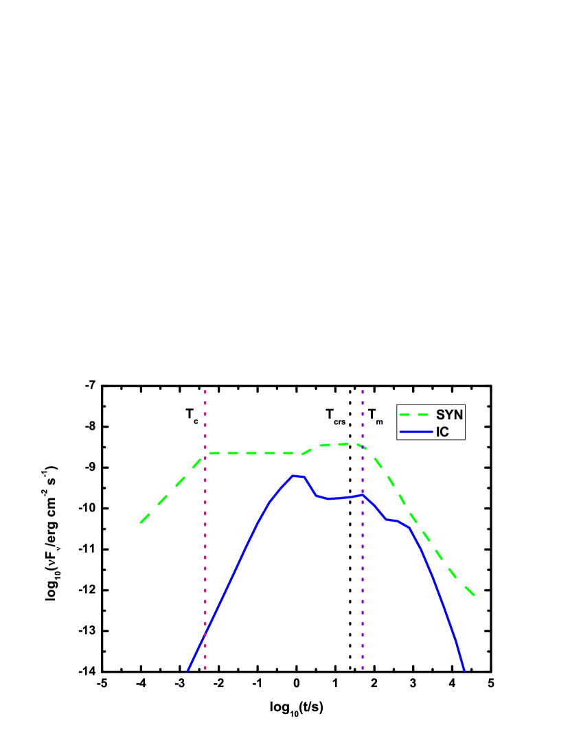
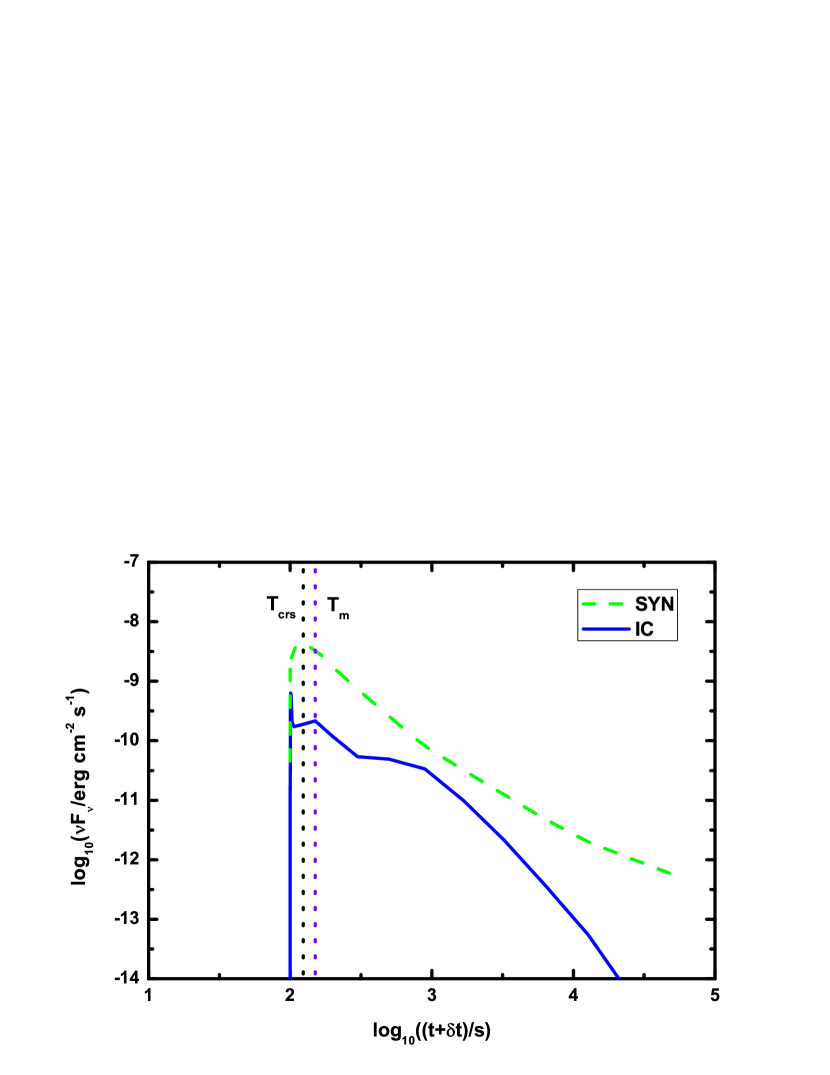
Figure 5: The light lines of the synchrotron and IC emission. The left panel is the flux verse time, and the right panel is obtained by resetting the time zero, where $\delta t=100\,$s is assumed. The green dashed line and the blue solid line represent the synchrotron emission and IC emission respectively. The three vertical dotted lines have the same meaning as in Fig. 2. The same parameters as in Fig. 1 are taken in numerical calculations.

References

- Abdo et al. (2011) Abdo, A. A. et al. 2011, ApJ, 734, L27
- Band et al. (1993) Band, D. et al. 1993, ApJ, 413, 281
- Blandford & McKee (1976) Blandford, R., & McKee, C. 1976, Phys. Fluids, 19, 1130
- Blumenthal & Gould (1970) Blumenthal, G. R., & Gould, R. J. 1970, Rev. Mod. Phys., 42, 237
- Burrows et al. (2005) Burrows, D. N., et al. 2005, Science, 309, 1833
- Dai & Lu (2002) Dai, Z. G., & Lu, T. 2002, ApJ, 580, 1013
- Dai et al. (2006) Dai, Z. G., Wang, X. Y., Wu, X. F., & Zhang, B. 2006, Science, 311, 1127
- Dermer et al. (2000) Dermer, C. D., Chiang, J., & Mitman, K. E. 2000, ApJ, 537, 785
- Fan & Piran (2006) Fan, Y. Z., Piran, T. 2006, MNRAS, 370, L24
- Fan et al. (2008) Fan, Y. Z., Piran, T., Narayan, R., & Wei, D. M. 2008, MNRAS, 384, 1483
- Fan & Wei (2005) Fan, Y. Z., & Wei, D. M. 2005, MNRAS, 364, L42
- Galli & Piro (2007) Galli, A., & Piro, L. 2007, A&A, 475, 421
- Gupta & Zhang (2007) Gupta, N., & Zhang, B. 2007, MNRAS, 380, 78
- He et al. (2012) He, H. N. et al. 2012, ApJ, 753, 178
- King et al. (2005) King, A., O’Brien, P. T., Goad, M. R., Osborne, J., Olsson, E., & Page, K. 2005, ApJ, 630, L113
- Lazzati & Perna (2007) Lazzati, D, & Perna, R. 2007, MNRAS, 375, L46
- Liang et al. (2006) Liang, E. W. et al. 2006, ApJ, 646, 351
- Lithwick & Sari (2001) Lithwick, Y. & Sari, R. 2001, ApJ, 555, 540
- Meszaros & Rees (1994) Meszaros, P., & Rees, M. J. 1994, MNRAS, 269, L41
- Meszaros & Rees & Papatheanassiou (1994) Meszaros, P., Rees, M. J., & Papathanassiou, H. 1994, ApJ, 432, 181
- Pe’er & Waxman (2005) Pe’er, A., & Waxman, E. 2005, ApJ, 633, 1018 (Erratum-ibid. 2006, ApJ, 638, 1187)
- Perna et al. (2006) Perna, R., Armitage, P. J., & Zhang, B. 2006, ApJ, 636, L29
- Piro et al. (2005) Piro, L., et al. 2005, ApJ, 623, 314
- Proga & Zhang (2006) Proga, D., & Zhang, B. 2006, MNRAS, 370, L61
- Rybicki & Lightman (1979) Rybicki, G. B., & Lightman, A. P. 1979, Radiative Processes in Astrophysics (New York: Wiley Interscience)
- Sari et al. (1998) Sari, R., Piran, T., & Narayan, R. 1998, ApJ, 497, L17
- Sari & Esin (2001) Sari, R., & Esin, A. A. 2001, ApJ, 548, 787
- Tavecchio et al. (1998) Tavecchio, F., Maraschi, L., & Ghisellini, G. 1998, ApJ, 509, 608
- Wang et al. (2001a) Wang, X. Y., Dai, Z. G., & Lu, T. 2001a, ApJ, 546, L33
- Wang et al. (2001b) Wang, X. Y., Dai, Z. G., & Lu, T. 2001b, ApJ, 556, 1010
- Wang et al. (2004) Wang, X. Y., Cheng, K. S., Dai, Z. G., & Lu, T. 2004, ApJ, 604, 306
- Wang et al. (2006) Wang, X. Y., Li, Z., & Meszaros, P. 2006, ApJ, 641, L89
- Wu et al. (2005) Wu, X.F., Dai, Z.G., Wang, X.Y., Huang, Y.F., Feng, L.L., & Lu, T. astro-ph/0512555
- Yu & Dai (2007) Yu, Y. W., & Dai, Z. G. 2007, A&A, 470, 119
- Yu & Dai (2009) Yu, Y. W., & Dai, Z. G. 2009, ApJ, 692, 133
- Zhang et al. (2006) Zhang, B. et al. 2006, ApJ, 642, 354
- Zhang & Meszaros (2001) Zhang, B., & Meszaros, P. 2001, ApJ, 559, 110
- Zhang (2007) Zhang, B. 2007, ChJAA, 7, 1