Subtraction method and stability condition
in the extended RPA theories

Abstract

The extended RPA theories are analyzed from the point of view of the problem of stability of their solutions. Three kinds of such theories are considered: the second RPA and two versions of the quasiparticle-phonon coupling model within the time-blocking approximation: the model including $1p1h\otimes$phonon configurations and the two-phonon model. It is shown that stability is ensured by making use of the subtraction method proposed previously to solve double counting problem in these theories. This enables one to generalize the famous Thouless theorem proved in the case of the RPA. These results are illustrated by an example of schematic model.

I Introduction

One of the trends in the modern nuclear structure theory is the calculations in a large model configuration space. On the one hand, this trend is caused by the requirement of the internal consistency of the theory. On the other hand, such calculations allow us in some cases to describe the nuclear structure effects which can not be reproduced within the framework of the more simple models. However, the use of the large configuration space leads to the problems of convergence and stability of the solutions obtained. It should be noted that, though the problems of convergence and stability are close to each other, they do not coincide. The convergence is understood in the usual mathematical sense, while stability, as applied to the description of the excited states, implies that all the calculated excitation energies should be real and positive.

The most widely used models, in which these problems can be resolved (or do not arise at all), are the Hartree-Fock (HF) approximation aimed at the description of the ground states and the random phase approximation (RPA) within which the characteristics of the excited states can be calculated (see RS80 ). Usually, these models are referred to as the mean-field theories. In particular, the problem of stability is resolved in the HF based self-consistent RPA as was shown by Thouless in Refs. Th60 ; Th61 . But these problems become actual and remain so far open in the models going beyond these approximations. The reasons for developing and using such extended models are well known (see, e.g., Ref. DNSW90 ). First of all, they are related to the fact that within the HF approximation and within the RPA one can not describe the effects of the fragmentation of the nuclear states leading to the formation of the so-called spreading widths of the resonances.

There is a series of models within which these effects are included. One of them is the second RPA (SRPA, see DNSW90 ; SW61 ; S62 ; YDG83 ). The problems mentioned above arise in this model because of enlarging the configuration space which includes two-particles–two-holes ($2p2h$) states in addition to the one-particle–one-hole ($1p1h$) states incorporated in the RPA. In Refs. PR09 ; PR10 ; GGC11 ; GGDDCC12 it was obtained that calculations of giant resonances in ¹⁶O, ⁴⁰Ca, ⁴⁸Ca, and ⁹⁰Zr within the SRPA lead to a very large (up to 10 MeV and more so) downward shifts of their centroids relatively to the RPA values if the size of the configuration space is sufficiently large. It was also found that some low-lying states in the SRPA become unstable, so the question arises as to whether the SRPA is applicable in the low-energy region (see PR10 ). In Refs. MGCG10 ; MGRMC12 the problem of the ultraviolet divergence appearing at the second order beyond the HF approximation was analyzed in the case of nuclear matter.

In the present paper we will consider in detail the problem of stability in the extended RPA (ERPA) theories. The problem of convergence will be only briefly touched upon. Note that the term ERPA is sometimes used with regard to the models taking into account the ground state correlations beyond the RPA (see, e.g., Refs. VKCS00 ; TS07 ). These effects will not be discussed here. The following models will be considered: the SRPA and two versions of the quasiparticle-phonon coupling model formulated within the Green function method on the basis of the time-blocking approximation (TBA): the model including $1p1h\otimes$phonon configurations TBA89 ; TBA97 ; KST04 and the two-phonon model QTBA1 . It will be shown that stability can be ensured by making use of the subtraction method QTBA1 . This method was applied in the calculations of giant resonances within the quasipartical TBA (QTBA) in QTBA2 ; ISGMR ; AGKK11 and within its relativistic generalization in RTBA ; RQTBA1 ; RQTBA2 to eliminate double counting in these models. However, it was not analyzed previously in the context of the stability issue.

The paper is organized as follows. In Sec. II the problem of stability and the content of the Thouless theorem in the RPA framework are considered. In Sec. III the response function formalism is outlined within which the stability problem is revealed in more detail. The ERPA theories mentioned above are briefly described in Sec. IV. In Sections V and VI the subtraction method and the stability condition in the ERPA are considered. The general results obtained in the previous sections are analyzed within the framework of the schematic model in Sec. VII. The conclusions are given in Sec. VIII.

II Thouless theorem

The Thouless theorem Th60 ; Th61 determines stability condition in the case of the self-consistent RPA. Let us briefly recall the structure of the RPA equations and the content of this theorem because its generalization to the case of the ERPA theories can be carried out (see Sec. VI) using a simple analogy.

To build the RPA equations one needs the single-particle density matrix $\rho^{\vphantom{*}}_{12}$, the single-particle Hamiltonian $h^{\vphantom{*}}_{12}$, and the amplitude of the residual interaction ${V}^{\vphantom{*}}_{12,34}$. Here and in the following the numerical indices ($1,2,3,\ldots$) stand for the sets of the quantum numbers of some single-particle basis. It is supposed that the following equalities are fulfilled

$$\rho^{2}=\rho\,,\qquad[\,h,\rho\,]=0\,.$$ (1)

Let us introduce the single-particle basis that diagonalizes operators $h$ and $\rho\,$:

$$h^{\vphantom{*}}_{12}=\varepsilon^{\vphantom{*}}_{1}\delta^{\vphantom{*}}_{12}\,,\qquad\rho^{\vphantom{*}}_{12}=n^{\vphantom{*}}_{1}\delta^{\vphantom{*}}_{12}$$ (2)

where $n^{\vphantom{*}}_{1}$ is the occupation number. In what follows the indices $p$ and $h$ will be used to label the single-particle states of the particles ($n^{\vphantom{*}}_{p}=0$) and holes ($n^{\vphantom{*}}_{h}=1$) in this basis. The matrix

$$M^{{}_{\mbox{\scriptsize RPA}}}_{12,34}=\delta^{\vphantom{*}}_{13}\,\rho^{\vphantom{*}}_{42}-\rho^{\vphantom{*}}_{13}\,\delta^{\vphantom{*}}_{42}$$ (3)

is the metric matrix in the RPA. The range of $M^{{}_{\mbox{\scriptsize RPA}}}_{\vphantom{1}}$ forms the $1p1h$ configuration space. The vectors $z^{\vphantom{*}}_{12}$ in this space have the components of $z^{\vphantom{*}}_{ph}$ and $z^{\vphantom{*}}_{hp}$ types. The RPA matrix $\Omega^{{}_{\mbox{\scriptsize RPA}}}_{12,34}$ acts in the $1p1h$ space. In the general case it has the form

$$\Omega^{{}_{\mbox{\scriptsize RPA}}}_{12,34}=h^{\vphantom{*}}_{13}\,\delta^{\vphantom{*}}_{42}-\delta^{\vphantom{*}}_{13}\,h^{\vphantom{*}}_{42}+\sum_{56}M^{{}_{\mbox{\scriptsize RPA}}}_{12,56}\,{V}^{\vphantom{*}}_{56,34}\,.$$ (4)

The RPA eigenvalue equation reads

$$\sum_{34}\Omega^{{}_{\mbox{\scriptsize RPA}}}_{12,34}\,z^{n}_{34}=\omega^{\vphantom{*}}_{n}\,z^{n}_{12}$$ (5)

where $\omega^{\vphantom{*}}_{n}$ is the excitation energy, $z^{n}_{12}$ is the transition amplitude. In the case of the self-consistent RPA, based on the energy density functional $E[\rho]$, the quantities $h$ and $V$ in Eq. (4) are linked by the equations

$$h^{\vphantom{*}}_{12}=\frac{\delta E[\rho]}{\delta\rho^{\vphantom{*}}_{21}}\,,\qquad{V}^{\vphantom{*}}_{12,34}=\frac{\delta^{2}E[\rho]}{\delta\rho^{\vphantom{*}}_{21}\,\delta\rho^{\vphantom{*}}_{34}}\,.$$ (6)

Eqs. (1) play the role of the equations of motion.

The Thouless theorem can be formulated in terms of the following general statement (see, e.g., Ref. RS80 ). Let a matrix $A$ be representable in the form $A=BC$ where the matrices $B$ and $C$ are Hermitian and $C$ is positive semidefinite (i.e., $\,\langle\,z\,|\,C\,|\,z\,\rangle\geqslant 0\,$ for any complex vector $|\,z\,\rangle$). Then all the eigenvalues of the matrix $A$ are real. Indeed, consider the eigenvalue equation

$$A\,|\,x\,\rangle=a\,|\,x\,\rangle\,.$$ (7)

From the positive semidefiniteness of the Hermitian matrix $C$ it follows that there exists Hermitian matrix $C^{1/2}$ such that $C=(C^{1/2})^{2}$. Let us denote $\,|\,y\,\rangle=C^{1/2}|\,x\,\rangle$. If $\,|\,y\,\rangle=0$ then $a=0$. If $\,|\,y\,\rangle\neq 0$ then, by multiplying Eq. (7) with $C^{1/2}$, we obtain $D\,|\,y\,\rangle=a\,|\,y\,\rangle$ where $D=C^{1/2}B\,C^{1/2}$. The matrix $D$ is Hermitian, consequently, the eigenvalue $a$ is real.

Coming back to Eq. (5), let us define the RPA stability matrix

$$\mathfrak{S}^{{}_{\mbox{\scriptsize RPA}}}_{\vphantom{1}}=M^{{}_{\mbox{\scriptsize RPA}}}_{\vphantom{1}}\Omega^{{}_{\mbox{\scriptsize RPA}}}_{\vphantom{1}}.$$ (8)

Since $(M^{{}_{\mbox{\scriptsize RPA}}}_{\vphantom{1}})^{2}=1$ in the $1p1h$ space, Eq. (8) is equivalent to the equation

$$\Omega^{{}_{\mbox{\scriptsize RPA}}}_{\vphantom{1}}=M^{{}_{\mbox{\scriptsize RPA}}}_{\vphantom{1}}\mathfrak{S}^{{}_{\mbox{\scriptsize RPA}}}_{\vphantom{1}}.$$ (9)

Now we note that both the matrix $M^{{}_{\mbox{\scriptsize RPA}}}_{\vphantom{1}}$ and the matrix $\mathfrak{S}^{{}_{\mbox{\scriptsize RPA}}}_{\vphantom{1}}$ in Eq. (9) are Hermitian. Therefore, all eigenvalues $\omega^{\vphantom{*}}_{n}$ in Eq. (5) are real if the stability matrix $\mathfrak{S}^{{}_{\mbox{\scriptsize RPA}}}_{\vphantom{1}}$ is positive semidefinite. This is the statement of the Thouless theorem. The positive semidefiniteness of the matrix $\mathfrak{S}^{{}_{\mbox{\scriptsize RPA}}}_{\vphantom{1}}$ follows from the conditions of minimization of the energy density functional $E[\rho]$ in the self-consistent theory (see RS80 ; Th60 ). Note that the matrix $\mathfrak{S}^{{}_{\mbox{\scriptsize RPA}}}_{\vphantom{1}}$ is not positive definite because of the symmetry properties of $E[\rho]$.

Reality of the eigenvalues in Eq. (5) leads to the following symmetry property of the solutions of this equation. Let us introduce the permutation operator acting in the space of the pairs of the single-particle indices: $\mathfrak{P}^{\vphantom{*}}_{12,34}=\delta^{\vphantom{*}}_{14}\delta^{\vphantom{*}}_{23}\,$. From the definitions (3), (4), and (6) it follows that $\Omega^{{}_{\mbox{\scriptsize RPA}}}_{\vphantom{1}}=-\mathfrak{P}\,\Omega^{{}_{\mbox{\scriptsize RPA}}*}_{\vphantom{1}}\mathfrak{P}$. This equality together with Eq. (5) and reality of $\omega^{\vphantom{*}}_{n}$ brings us to the equation

$$|\,z^{-n}\rangle=\mathfrak{P}\,|\,z^{n}\rangle^{*}$$ (10)

where the eigenvectors $|\,z^{n}\rangle$ and $|\,z^{-n}\rangle$ correspond to the eigenvalues $\omega^{\vphantom{*}}_{n}$ and $-\omega^{\vphantom{*}}_{n}$, respectively.

III Response function formalism

The other important consequences of the positive semidefiniteness of the stability matrix which will be used in the following in the context of the ERPA theories concern the properties of the response function $R(\omega)$ defined in the RPA by the equation

$$R^{{}_{\mbox{\scriptsize RPA}}}_{\vphantom{1}}(\omega)=-\bigl{(}\,\omega-\Omega^{{}_{\mbox{\scriptsize RPA}}}_{\vphantom{1}}\bigr{)}^{-1}M^{{}_{\mbox{\scriptsize RPA}}}_{\vphantom{1}}.$$ (11)

An overall sign in this formula is chosen in accordance with the usual definition of the response function in the Green function method (see Ref. SWW77 ). The response function formalism is a conventional tool for the description of nuclear excitations. In the general case the distribution of the strength of transitions in the nucleus caused by some external field represented by the single-particle operator $Q$ is determined by the (dynamic) polarizability $\Pi(\omega)$ which is defined in terms of the response function as

$$\Pi(\omega)=-\langle\,Q\,|\,R(\omega)\,|\,Q\,\rangle\,.$$ (12)

The poles and residua of the function $\Pi(\omega)$ coincide with the excitation energies and the transition probabilities (see Eq. (30) below).

Let us introduce an auxiliary matrix

$$\tilde{\mathfrak{S}}^{{}_{\mbox{\scriptsize RPA}}}_{\vphantom{1}}=\mathfrak{S}^{{}_{\mbox{\scriptsize RPA}}}_{\vphantom{1}}+\delta$$ (13)

where $\delta$ is a real positive number. If $\mathfrak{S}^{{}_{\mbox{\scriptsize RPA}}}_{\vphantom{1}}$ is positive semidefinite, then the matrix $\tilde{\mathfrak{S}}^{{}_{\mbox{\scriptsize RPA}}}_{\vphantom{1}}$ is positive definite and consequently there exists invertible Hermitian matrix $\tilde{\mathfrak{S}}^{1/2}$ such that $\tilde{\mathfrak{S}}^{{}_{\mbox{\scriptsize RPA}}}_{\vphantom{1}}=(\tilde{\mathfrak{S}}^{1/2})^{2}$. Let us denote: $\tilde{\Omega}^{{}_{\mbox{\scriptsize RPA}}}_{\vphantom{1}}=M^{{}_{\mbox{\scriptsize RPA}}}_{\vphantom{1}}\tilde{\mathfrak{S}}^{{}_{\mbox{\scriptsize RPA}}}_{\vphantom{1}}$,

$$\tilde{R}^{{}_{\mbox{\scriptsize RPA}}}_{\vphantom{1}}(\omega)=-\bigl{(}\,\omega-\tilde{\Omega}^{{}_{\mbox{\scriptsize RPA}}}_{\vphantom{1}}\bigr{)}^{-1}M^{{}_{\mbox{\scriptsize RPA}}}_{\vphantom{1}}.$$ (14)

Using the invertibility of the matrix $\tilde{\mathfrak{S}}^{1/2}$ we obtain

$$\tilde{R}^{{}_{\mbox{\scriptsize RPA}}}_{\vphantom{1}}(\omega)$$

$$=-(\tilde{\mathfrak{S}}^{1/2})^{-1}\bigl{(}\,\omega-\tilde{H}^{{}_{\mbox{\scriptsize RPA}}}_{\vphantom{1}}\bigr{)}^{-1}\tilde{H}^{{}_{\mbox{\scriptsize RPA}}}_{\vphantom{1}}\,(\tilde{\mathfrak{S}}^{1/2})^{-1}$$ (15)

where $\tilde{H}^{{}_{\mbox{\scriptsize RPA}}}_{\vphantom{1}}=\tilde{\mathfrak{S}}^{1/2}M^{{}_{\mbox{\scriptsize RPA}}}_{\vphantom{1}}\tilde{\mathfrak{S}}^{1/2}$. The matrices $\tilde{\Omega}^{{}_{\mbox{\scriptsize RPA}}}_{\vphantom{1}}$ and $\tilde{H}^{{}_{\mbox{\scriptsize RPA}}}_{\vphantom{1}}$ have the same set of the (non-zero) eigenvalues $\{\,\tilde{\omega}^{\vphantom{*}}_{n}\}$. But, in contrast to $\tilde{\Omega}^{{}_{\mbox{\scriptsize RPA}}}_{\vphantom{1}}$, the matrix $\tilde{H}^{{}_{\mbox{\scriptsize RPA}}}_{\vphantom{1}}$ is Hermitian.

Let $\{\,|\,\tilde{y}^{n}\rangle\}$ be a complete set of the orthonormalized eigenvectors of the matrix $\tilde{H}^{{}_{\mbox{\scriptsize RPA}}}_{\vphantom{1}}$. Insertion of the sum $\sum_{n}|\,\tilde{y}^{n}\rangle\langle\,\tilde{y}^{n}|=1$ into Eq. (15) yields

$$\tilde{R}^{{}_{\mbox{\scriptsize RPA}}}_{\vphantom{1}}(\omega)=-\sum_{n}\frac{\mbox{sgn}(\tilde{\omega}^{\vphantom{*}}_{n})\,|\,\tilde{z}^{n}\rangle\langle\tilde{z}^{n}|}{\omega-\tilde{\omega}^{\vphantom{*}}_{n}}$$ (16)

where

$$|\,\tilde{z}^{n}\rangle = \sqrt{|\,\tilde{\omega}^{\vphantom{*}}_{n}|}\,(\tilde{\mathfrak{S}}^{1/2})^{-1}|\,\tilde{y}^{n}\rangle$$ (17)

$$= \frac{\mbox{sgn}(\tilde{\omega}^{\vphantom{*}}_{n})}{\sqrt{|\,\tilde{\omega}^{\vphantom{*}}_{n}}|}\;M^{{}_{\mbox{\scriptsize RPA}}}_{\vphantom{1}}\,\tilde{\mathfrak{S}}^{1/2}\,|\,\tilde{y}^{n}\rangle\,,$$

$$\tilde{\Omega}^{{}_{\mbox{\scriptsize RPA}}}_{\vphantom{1}}|\,\tilde{z}^{n}\rangle=\tilde{\omega}^{\vphantom{*}}_{n}\,|\,\tilde{z}^{n}\rangle\,,$$ (18)

$$\langle\,\tilde{z}^{n}\,|\,M^{{}_{\mbox{\scriptsize RPA}}}_{\vphantom{1}}|\,\tilde{z}^{n^{\prime}}\rangle=\mbox{sgn}(\tilde{\omega}^{\vphantom{*}}_{n})\,\delta^{\vphantom{*}}_{n,\,n^{\prime}}\,.$$ (19)

Now, going to the limit $\delta\rightarrow+0$, we obtain

$$R^{\,\mbox{\scriptsize RPA}}_{\vphantom{1}}(\omega)=R^{\,\mbox{\scriptsize RPA(0)}}(\omega)-{\sum_{n}}^{\,\prime}\frac{\;\mbox{sgn}(\omega^{\vphantom{*}}_{n})\,a^{n}}{\omega-\omega^{\vphantom{*}}_{n}}$$ (20)

where

$$R^{\,\mbox{\scriptsize RPA(0)}}(\omega)=-\sum_{k=1}^{2}\,\frac{a^{(\,0,k)}}{\omega^{k}}\,,$$ (21)

$$a^{(\,0,k)}=\lim_{\delta\rightarrow+0}\;{\sum_{n}}^{(0)}\mbox{sgn}(\tilde{\omega}^{\vphantom{*}}_{n})\,\tilde{\omega}^{k-1}_{n}\,|\,\tilde{z}^{n}\rangle\langle\tilde{z}^{n}|\,,$$ (22)

$$a^{n}=|\,z^{n}\rangle\langle z^{n}|\,.$$ (23)

Symbol ${\sum}^{(0)}$ in Eq. (22) means the sum over all the states $n$ for which $\tilde{\omega}^{\vphantom{*}}_{n}\rightarrow\pm 0$ at $\delta\rightarrow+0$ (that is over the spurious states). Symbol ${\sum}^{\,\prime}$ in Eq. (20) means the sum over all the states $n$ excluding the spurious states. Note that the sum over $k$ in Eq. (21) is limited to the first two terms because, as follows from Eqs. (17) and (22), $a^{(\,0,k)}=0$ at $k>2$.

The non-spurious eigenvectors $|\,z^{n}\rangle$ satisfy Eq. (5) and are normalized by the condition

$$\langle\,{z}^{n}\,|\,M^{{}_{\mbox{\scriptsize RPA}}}_{\vphantom{1}}|\,{z}^{n^{\prime}}\rangle=\mbox{sgn}(\omega^{\vphantom{*}}_{n})\,\delta^{\vphantom{*}}_{n,\,n^{\prime}}$$ (24)

following from Eq. (19). The matrices $a^{(\,0,1)}$ and $a^{(\,0,2)}$ are Hermitian and satisfy the equations

$$\Omega^{{}_{\mbox{\scriptsize RPA}}}_{\vphantom{1}}a^{(\,0,1)}=a^{(\,0,2)},\quad\Omega^{{}_{\mbox{\scriptsize RPA}}}_{\vphantom{1}}a^{(\,0,2)}=0\,,$$ (25)

$$a^{(\,0,1)}M^{{}_{\mbox{\scriptsize RPA}}}_{\vphantom{1}}\,a^{(\,0,k)}=a^{(\,0,k)},$$ (26)

$$a^{(\,0,1)}=-\mathfrak{P}\,a^{(\,0,1)*}\mathfrak{P},\quad a^{(\,0,2)}=\mathfrak{P}\,a^{(\,0,2)*}\mathfrak{P}$$ (27)

following from Eqs. (10), (18), (19), and (22). The closure relation

$$a^{(\,0,1)}+{\sum_{n}}^{\,\prime}\mbox{sgn}(\omega^{\vphantom{*}}_{n})\,a^{n}=M^{{}_{\mbox{\scriptsize RPA}}}_{\vphantom{1}}$$ (28)

follows from Eqs. (11), (20), and (21).

Eq. (23) implies that all the matrices $a^{n}$ in the expansion (20) are Hermitian and positive semidefinite. In addition from Eqs. (10) and (23) we get

$$a^{-n}=\mathfrak{P}\;a^{n\,*}\,\mathfrak{P}\,.$$ (29)

These properties of the residua of the function $R^{{}_{\mbox{\scriptsize RPA}}}_{\vphantom{1}}(\omega)$ coincide with the properties of the exact response function following from its spectral representation (see, e.g., Ref. RS80 ). Taking this into account and making use of Eq. (12) we obtain that

$$\Pi^{{}_{\mbox{\scriptsize RPA}}}_{\vphantom{1}}(\omega)={\sum_{n}}^{\,\prime}\frac{\;\mbox{sgn}(\omega^{\vphantom{*}}_{n})B^{\vphantom{*}}_{\,n}(Q)}{\omega-\omega^{\vphantom{*}}_{n}}$$ (30)

where transition probabilities $B^{\vphantom{*}}_{\,n}(Q)=\langle\,Q\,|\,a^{n}\,|\,Q\,\rangle$ are real and non-negative and it is supposed that

$$\langle\,Q\,|\,a^{(\,0,k)}\,|\,Q\,\rangle=0\,,\quad k=1,2\,.$$ (31)

From Eq. (29) we also obtain that $B^{\vphantom{*}}_{-n}(Q)=B^{\vphantom{*}}_{\,n}(Q^{{\dagger}})$.

If the stability matrix does not possess the property of the positive semidefiniteness, the reality of the RPA eigenvalues $\omega^{\vphantom{*}}_{n}$ and the Hermiticity and the positive semidefiniteness of the matrices $a^{n}$ are not guaranteed. In particular, this means that the eigenvectors with positive eigenvalues may have negative norms. As a consequence, the reality and the non-negativeness of the RPA transition probabilities $B^{\vphantom{*}}_{\,n}(Q)$ in Eq. (30) is also not guaranteed, and the strength function

$$S^{{}_{\mbox{\scriptsize RPA}}}_{\vphantom{1}}(E,\Delta)=-\frac{1}{\pi}\;\mbox{Im}\,\Pi^{{}_{\mbox{\scriptsize RPA}}}_{\vphantom{1}}(E+i\Delta)$$ (32)

may take negative values at $E>0$ and $\Delta>0$. Note that the problem of the “negative transition probabilities” arising in this case can be treated as the problem of the “negative energies” since the function $\Pi^{{}_{\mbox{\scriptsize RPA}}}_{\vphantom{1}}(\omega)$ will have positive residua at the poles $\omega=\omega^{\vphantom{*}}_{n}<0$.

IV Extended RPA

In the ERPA theories the eigenvalue equation (5) is usually replaced (see, e.g., DNSW90 ) by the equation with the energy-dependent matrix $\Omega^{{}_{\mbox{\scriptsize ERPA}}}_{\vphantom{1}}(\omega)$:

$$\sum_{34}\Omega^{{}_{\mbox{\scriptsize ERPA}}}_{12,34}(\omega^{\vphantom{*}}_{\nu})\,z^{\nu}_{34}=\omega^{\vphantom{*}}_{\nu}\,z^{\nu}_{12}$$ (33)

where $\Omega^{{}_{\mbox{\scriptsize ERPA}}}_{\vphantom{1}}(\omega)$ can be represented in the form

$$\Omega^{{}_{\mbox{\scriptsize ERPA}}}_{\vphantom{1}}(\omega)=\Omega^{{}_{\mbox{\scriptsize RPA}}}_{\vphantom{1}}+M^{{}_{\mbox{\scriptsize RPA}}}_{\vphantom{1}}\,{W}(\omega)$$ (34)

and it is supposed that Eqs. (33) and (34) are written in the $1p1h$ subspace. The matrix ${W}(\omega)$ is the interaction amplitude that includes contributions of complex ($2p2h$) configurations. It has the following generic form

$${W}(\omega)={F}(\,\omega-M^{{}_{\mbox{\scriptsize C}}}_{\vphantom{1}}{\mathfrak{S}}^{{}_{\mbox{\scriptsize C}}}_{\vphantom{1}}\,)^{-1}M^{{}_{\mbox{\scriptsize C}}}_{\vphantom{1}}{F}^{{\dagger}}$$ (35)

where ${\mathfrak{S}}^{\mbox{\scriptsize C}}$, $M^{{}_{\mbox{\scriptsize C}}}_{\vphantom{1}}$, and ${F}$ are the block matrices of the form

$${\mathfrak{S}}^{{}_{\mbox{\scriptsize C}}}_{\vphantom{1}}=\left(\begin{array}[]{cc}{\mathfrak{S}}^{\mbox{\scriptsize C}(+)}&0\\ 0&{\mathfrak{S}}^{\mbox{\scriptsize C}(-)}\\ \end{array}\right),\quad M^{{}_{\mbox{\scriptsize C}}}_{\vphantom{1}}=\left(\begin{array}[]{rr}1&0\\ 0&-1\\ \end{array}\right),$$ (36)

${F}=\bigl{(}\,{F}^{(+)},{F}^{(-)}\bigr{)}$. The Hermitian matrices ${\mathfrak{S}}^{\mbox{\scriptsize C}(\pm)}$, ${\mathfrak{S}}^{\mbox{\scriptsize C}}$, and $M^{{}_{\mbox{\scriptsize C}}}_{\vphantom{1}}$ act in the subspace of complex configurations. The matrices ${F}$ and ${F}^{{\dagger}}$ connect this subspace with the $1p1h$ subspace. The matrices ${\mathfrak{S}}^{\mbox{\scriptsize C}}$ and $M^{\mbox{\scriptsize C}}$ play the role of the stability matrix and the metric matrix in the $2p2h$ subspace, respectively. In addition, the following equalities are fulfilled

$${\mathfrak{S}}^{\mbox{\scriptsize C}(-)}={\mathfrak{S}}^{\mbox{\scriptsize C}(+)*},\quad{F}^{(-)}=\mathfrak{P}\,{F}^{(+)*},$$ (37)

$$M^{{}_{\mbox{\scriptsize RPA}}}_{\vphantom{1}}{F}^{(\pm)}=\pm\,{F}^{(\pm)}.$$ (38)

Eqs. (37) lead to the symmetry property

$$\Omega^{{}_{\mbox{\scriptsize ERPA}}}_{\vphantom{1}}(\omega)=-\mathfrak{P}\,\Omega^{{}_{\mbox{\scriptsize ERPA}}*}_{\vphantom{1}}(-\omega^{*})\mathfrak{P}$$ (39)

from which we obtain for the eigenvectors with the real eigenvalues in Eq. (33) the following relation

$$|\,z^{-\nu}\rangle=\mathfrak{P}\,|\,z^{\nu}\rangle^{*},$$ (40)

where $|\,z^{-\nu}\rangle$ is the eigenvector with the eigenvalue $-\omega^{\vphantom{*}}_{\nu}\,$, as in the case of the RPA, see Eq. (10).

Using the complete sets of the eigenvectors of the matrices ${\mathfrak{S}}^{\mbox{\scriptsize C}(\pm)}$ one can represent Eq. (35) in the more explicit form:

$${W}^{\vphantom{*}}_{12,34}(\omega)=\sum_{c,\;\sigma}\,\frac{\sigma\,{F}^{c(\sigma)}_{12}{F}^{c(\sigma)*}_{34}}{\omega-\sigma\,\Omega^{\vphantom{*}}_{c}}$$ (41)

where $\sigma=\pm 1$, $c$ is an index of the subspace of complex configurations, $\Omega^{\vphantom{*}}_{c}$ are the eigenvalues of the matrices ${\mathfrak{S}}^{\mbox{\scriptsize C}(\pm)}$. It is supposed that the matrices ${\mathfrak{S}}^{\mbox{\scriptsize C}(\pm)}$ are positive definite and, consequently, $\Omega^{\vphantom{*}}_{c}>0$. Consider three models which can be formulated using Eq. (41) for the matrix ${W}(\omega)$. From Eqs. (37) and (38) it follows that ${F}^{c(-)}_{12}={F}^{c(+)*}_{21}$ and ${F}^{c(-)}_{ph}={F}^{c(+)}_{hp}=0$. So only the quantities ${F}^{c(+)}_{ph}$ and the energies $\Omega^{\vphantom{*}}_{c}$ should be specified.

(a) Second RPA in the so-called diagonal approximation DNSW90 ; YDG83 ; PR09 ; PR10 ; GGC11 ; GGDDCC12 . In this case one can set $c=\{p^{\prime},p^{\prime\prime},h^{\prime},h^{\prime\prime}\}$,

$$\Omega^{\vphantom{*}}_{c}=\varepsilon^{\vphantom{*}}_{p^{\prime}}+\varepsilon^{\vphantom{*}}_{p^{\prime\prime}}-\varepsilon^{\vphantom{*}}_{h^{\prime}}-\varepsilon^{\vphantom{*}}_{h^{\prime\prime}}\,,$$ (42)

$${F}^{c(+)}_{ph} = \frac{1}{2}\;\biggl{(}\,\delta^{\vphantom{*}}_{pp^{\prime}}\,w^{\vphantom{*}}_{h^{\prime}h^{\prime\prime},\;p^{\prime\prime}h}-\delta^{\vphantom{*}}_{pp^{\prime\prime}}\,w^{\vphantom{*}}_{h^{\prime}h^{\prime\prime},\;p^{\prime}h}$$ (43)

$$+ \delta^{\vphantom{*}}_{hh^{\prime}}\,w^{\vphantom{*}}_{ph^{\prime\prime},\;p^{\prime}p^{\prime\prime}}-\delta^{\vphantom{*}}_{hh^{\prime\prime}}\,w^{\vphantom{*}}_{ph^{\prime},\;p^{\prime}p^{\prime\prime}}\,\biggr{)}$$

where $w^{\vphantom{*}}_{12,34}=-w^{\vphantom{*}}_{21,34}=-w^{\vphantom{*}}_{12,43}$ is an antisymmetrized amplitude of the two-particle interaction. In the first order we have ${V}^{\vphantom{*}}_{12,34}=w^{\vphantom{*}}_{14,23}\,$, however in the general case the amplitude of the residual interaction in Eq. (6) does not coincide with $w$ and is not antisymmetric. Note that the full SRPA scheme is usually formulated by means of the equations similar to Eq. (35).

(b) TBA1: the quasiparticle-phonon coupling model within the TBA including $1p1h\otimes$phonon configurations TBA89 ; TBA97 ; KST04 (without ground state correlations beyond the RPA included in TBA89 ; TBA97 ; KST04 ). In this case $c=\{p^{\prime},h^{\prime},n\}$ where $n$ is the phonon’s index,

$$\Omega^{\vphantom{*}}_{c}=\varepsilon^{\vphantom{*}}_{p^{\prime}}-\varepsilon^{\vphantom{*}}_{h^{\prime}}+\omega^{\vphantom{*}}_{n}\,,\quad\omega^{\vphantom{*}}_{n}>0\,,$$ (44)

$${F}^{c(+)}_{ph}=\delta^{\vphantom{*}}_{pp^{\prime}}\,g^{n}_{h^{\prime}h}-\delta^{\vphantom{*}}_{h^{\prime}h}\,g^{n}_{pp^{\prime}},$$ (45)

$g^{n}_{12}$ is an amplitude of the quasiparticle-phonon interaction. In the self-consistent approach, these amplitudes (along with the phonon’s energies $\omega^{\vphantom{*}}_{n}$) are determined by the positive frequency solutions of the RPA equations (5) and (24) according to the formula

$$g^{n}_{12}=\sum_{34}{V}^{\vphantom{*}}_{12,34}\,z^{n}_{34}.$$ (46)

Physical effects taken into account in the TBA1 and the general structure of the equations are the same as in the particle-vibration coupling model W85 and in the model of the coupling of $1p1h$ configurations to the doorway states CGBB94 .

(c) TBA2: the quasiparticle-phonon coupling model within the TBA including two-phonon configurations QTBA1 . This model is a straightforward generalization of the TBA1 by including additional correlations between particles and holes entering $1p1h\otimes$phonon configurations (but also without ground state correlations beyond the RPA and without pairing correlations included in QTBA1 ). Physically, this is similar, but not equivalent in details, to the first versions of the Quasiparticle-Phonon Model S92 . Relativistic extension of the two-phonon model was developed in Ref. RQTBA2 . In the TBA2 we have: $c=\{n,n^{\prime}\}$ where $n$ and $n^{\prime}$ are the phonon’s indices,

$$\Omega^{\vphantom{*}}_{c}=\omega^{\vphantom{*}}_{n}+\omega^{\vphantom{*}}_{n^{\prime}}\,,\quad\omega^{\vphantom{*}}_{n}>0\,,\quad\omega^{\vphantom{*}}_{n^{\prime}}>0\,,$$ (47)

$${F}^{c(+)}_{ph}=\sum_{p^{\prime\prime}h^{\prime\prime}}\bigl{(}\,\delta^{\vphantom{*}}_{pp^{\prime\prime}}\,g^{n}_{h^{\prime\prime}h}-\delta^{\vphantom{*}}_{h^{\prime\prime}h}\,g^{n}_{pp^{\prime\prime}}\,\bigr{)}\,z^{n^{\prime}}_{p^{\prime\prime}h^{\prime\prime}}\,.$$ (48)

The amplitudes $g^{n}_{12}$, $z^{n^{\prime}}_{12}$ and the phonon’s energies are determined by Eqs. (5), (24), and (46), as in the TBA1.

Obviously, the TBA2 reduces to the TBA1 in the case when the second phonon is non-collective, i.e., when $\omega^{\vphantom{*}}_{n^{\prime}}=\varepsilon^{\vphantom{*}}_{p^{\prime}}-\varepsilon^{\vphantom{*}}_{h^{\prime}}$ in Eq. (47) and $z^{n^{\prime}}_{p^{\prime\prime}h^{\prime\prime}}=\delta^{\vphantom{*}}_{p^{\prime\prime}p^{\prime}}\,\delta^{\vphantom{*}}_{h^{\prime\prime}h^{\prime}}$ in Eq. (48). However, the connection between the TBA1 and the SRPA is not so simple because of the well-known problem of the second order contributions arising in the quasiparticle-phonon coupling model (see, e.g., Ref. MBBD85 ).

V Subtraction method

The starting point of the ERPA theories is the usual RPA. In many practically significant cases (except for the so-called ab initio approaches) the self-consistent RPA is based on the density functional theory (DFT, see, e.g., Refs. E03 ; BHR03 ; DFP10 ) in which the energy density functional $E[\rho]$ is constructed in such a way as to provide an optimal (exact in the limiting case) description of the nuclear ground-state properties. Therefore, $E[\rho]$ already effectively contains a part of the contributions of those complex configurations which are explicitly included in the ERPA. This part can be treated as the static contributions, in contrast to the dynamic ones which lead to the formation of the spreading widths of the resonances. To avoid double counting, these static contributions in the ERPA should be eliminated. A simple way to do this is to impose the condition:

$$\Omega^{{}_{\mbox{\scriptsize ERPA}}}_{\vphantom{1}}(0)=\Omega^{{}_{\mbox{\scriptsize RPA}}}_{\vphantom{1}}\,.$$ (49)

The reasons for this condition are as follows. Let $Q$ be a local Hermitian single-particle operator representing some external field. Dynamic polarizability $\Pi(\omega)$ corresponding to this field is defined by Eq. (12) in which the response function $R(\omega)$ is defined by Eq. (11) in the RPA and by the equation

$$R^{{}_{\mbox{\scriptsize ERPA}}}_{\vphantom{1}}(\omega)=-\bigl{(}\,\omega-\Omega^{{}_{\mbox{\scriptsize ERPA}}}_{\vphantom{1}}(\omega)\,\bigr{)}^{-1}M^{{}_{\mbox{\scriptsize RPA}}}_{\vphantom{1}}$$ (50)

in the ERPA. Consider an energy density functional

$${\cal E}[\rho,\lambda]=E[\rho]+\lambda\,\mbox{Tr}\,\bigl{(}\rho\,Q\bigr{)}$$ (51)

where $\lambda$ is a real parameter. According to the so-called dielectric theorem BLM79 , we have:

$$\Pi^{{}_{\mbox{\scriptsize RPA}}}_{\vphantom{1}}(0)=-2m^{{}_{\mbox{\scriptsize RPA}}}_{-1}=\biggl{(}\frac{d}{d\lambda}\mbox{Tr}\,\bigl{(}\rho^{(\lambda)}Q\bigr{)}\biggr{)}_{\lambda=0}$$ (52)

where $\Pi^{{}_{\mbox{\scriptsize RPA}}}_{\vphantom{1}}(0)$ is the (static) polarizability calculated by making use of Eqs. (3), (4), (6), (11), and (12) in the self-consistent RPA based on the functional $E[\rho]$, the quantity $m^{{}_{\mbox{\scriptsize RPA}}}_{-1}$ is the inverse energy-weighted moment of the strength distribution in the RPA, $\rho^{(\lambda)}$ is the equilibrium density matrix of the functional ${\cal E}[\rho,\lambda]$, and it is supposed that $a^{(\,0,1)}|\,Q\,\rangle=0$. Assuming, in accordance with general principles of the DFT, that this theory gives in a sense an exact value of the quantity $\mbox{Tr}\,\bigl{(}\rho^{(\lambda)}Q\bigr{)}$ at any $\lambda$ near the point $\lambda=0$, one can consider that $\Pi^{{}_{\mbox{\scriptsize RPA}}}_{\vphantom{1}}(0)=-2m^{\vphantom{*}}_{-1}$ where $m^{\vphantom{*}}_{-1}$ is the exact inverse energy-weighted moment of the strength distribution including contributions of all configurations. Then, the condition $\Pi^{{}_{\mbox{\scriptsize ERPA}}}_{\vphantom{1}}(0)=\Pi^{{}_{\mbox{\scriptsize RPA}}}_{\vphantom{1}}(0)$ is natural and from this, using Eqs. (11), (12), and (50), we arrive at the condition (49). This condition will be fulfilled if we change the definition of the matrix $\Omega^{{}_{\mbox{\scriptsize ERPA}}}_{\vphantom{1}}(\omega)$ taking instead of Eq. (34) the following ansatz

$$\Omega^{{}_{\mbox{\scriptsize ERPA}}}_{\vphantom{1}}(\omega)=\Omega^{{}_{\mbox{\scriptsize RPA}}}_{\vphantom{1}}+M^{{}_{\mbox{\scriptsize RPA}}}_{\vphantom{1}}\bigl{[}\,{W}(\omega)-\kappa\,{W}(0)\,\bigr{]}$$ (53)

and setting $\kappa=1$.

Thus, the method of eliminating the double counting consists in subtracting the static part ${W}(0)$ from the interaction amplitude ${W}(\omega)$ containing the contributions of complex configurations. This method was used in the calculations of giant resonances both within self-consistent ISGMR ; AGKK11 ; RTBA ; RQTBA1 ; RQTBA2 and within non-self-consistent QTBA2 approaches. In the non-self-consistent models the problem of double counting arises because of the use of the phenomenologically fitted mean field and the residual interaction. In this case the subtraction method plays the same role as the so-called refinement procedure applied in Refs. DNSW90 ; TBA89 ; TBA97 ; KST04 .

VI Stability condition in the extended RPA theories

To analyze the properties of Eq. (33) with the matrix $\Omega^{{}_{\mbox{\scriptsize ERPA}}}_{\vphantom{1}}(\omega)$ defined by Eqs. (53), (35), and (36) let us recast Eq. (33) in the extended space including $1p1h$ and complex ($2p2h$) configurations. Let us define the energy-independent matrix $\widehat{\Omega}^{{}_{\mbox{\scriptsize ERPA}}}_{\vphantom{1}}$ in this space as the block matrix of the following form

$$\widehat{\Omega}^{{}_{\mbox{\scriptsize ERPA}}}_{\vphantom{1}}=\left(\begin{array}[]{cc}\Omega^{\mbox{\scriptsize RPA}(\kappa)}&\;M^{{}_{\mbox{\scriptsize RPA}}}_{\vphantom{1}}{F}\\ M^{{}_{\mbox{\scriptsize C}}}_{\vphantom{1}}{F}^{{\dagger}}&\;M^{{}_{\mbox{\scriptsize C}}}_{\vphantom{1}}{\mathfrak{S}}^{{}_{\mbox{\scriptsize C}}}_{\vphantom{1}}\\ \end{array}\right)$$ (54)

where

$$\Omega^{\mbox{\scriptsize RPA}(\kappa)}=\Omega^{{}_{\mbox{\scriptsize RPA}}}_{\vphantom{1}}+\kappa\,M^{{}_{\mbox{\scriptsize RPA}}}_{\vphantom{1}}{F}\,({\mathfrak{S}}^{{}_{\mbox{\scriptsize C}}}_{\vphantom{1}})^{-1}{F}^{{\dagger}}.$$ (55)

It is easy to verify that Eq. (33) is equivalent to the following linear eigenvalue equation

$$\widehat{\Omega}^{{}_{\mbox{\scriptsize ERPA}}}_{\vphantom{1}}\,|\,Z^{\,\nu}_{\vphantom{1}}\rangle=\omega^{\vphantom{*}}_{\nu}\,|\,Z^{\,\nu}_{\vphantom{1}}\rangle$$ (56)

where

$$|\,Z^{\,\nu}_{\vphantom{1}}\rangle=\left(\begin{array}[]{c}|\,z^{\,\nu}_{\vphantom{1}}\rangle\vphantom{\frac{A}{B}}\\ |\,\zeta^{\,\nu}_{\vphantom{1}}\rangle\vphantom{\frac{A}{B}}\\ \end{array}\right).$$ (57)

The vector $|\,z^{\,\nu}_{\vphantom{1}}\rangle$ in Eq. (57) belongs to the $1p1h$ subspace and coincides with the vector in Eq. (33). The vector $|\,\zeta^{\,\nu}_{\vphantom{1}}\rangle$ belongs to the subspace of complex configurations.

The matrix $\widehat{\Omega}^{{}_{\mbox{\scriptsize ERPA}}}_{\vphantom{1}}$ can be represented in the form $\widehat{\Omega}^{{}_{\mbox{\scriptsize ERPA}}}_{\vphantom{1}}={M}^{{}_{\mbox{\scriptsize ERPA}}}_{\vphantom{1}}\mathfrak{S}^{{}_{\mbox{\scriptsize ERPA}}}_{\vphantom{1}}$ where

$${M}^{{}_{\mbox{\scriptsize ERPA}}}_{\vphantom{1}}=\left(\begin{array}[]{cc}M^{{}_{\mbox{\scriptsize RPA}}}_{\vphantom{1}}&0\\ 0\hphantom{A}&M^{{}_{\mbox{\scriptsize C}}}_{\vphantom{1}}\\ \end{array}\right)$$ (58)

is the metric matrix, $\mathfrak{S}^{{}_{\mbox{\scriptsize ERPA}}}_{\vphantom{1}}$ is the stability matrix in the ERPA which is defined in analogy to Eq. (8):

$$\mathfrak{S}^{{}_{\mbox{\scriptsize ERPA}}}_{\vphantom{1}}={M}^{{}_{\mbox{\scriptsize ERPA}}}_{\vphantom{1}}\,\widehat{\Omega}^{{}_{\mbox{\scriptsize ERPA}}}_{\vphantom{1}}.$$ (59)

Using Eqs. (54), (55), (58), and (59) we obtain that for any complex vector $|Z\,\rangle$,

$$|Z\,\rangle=\left(\begin{array}[]{c}|\,z\,\rangle\vphantom{\frac{A}{B}}\\ |\,\zeta\,\rangle\vphantom{\frac{A}{B}}\\ \end{array}\right),$$ (60)

with arbitrary components $|\,z\,\rangle$ and $|\,\zeta\,\rangle$ the following equation is fulfilled

$$\langle\,Z\,|\,\mathfrak{S}^{{}_{\mbox{\scriptsize ERPA}}}_{\vphantom{1}}|Z\,\rangle = \langle\,z\,|\,\mathfrak{S}^{{}_{\mbox{\scriptsize RPA}}}_{\vphantom{1}}|\,z\,\rangle+\langle\,\zeta^{\prime}|\,{\mathfrak{S}}^{{}_{\mbox{\scriptsize C}}}_{\vphantom{1}}|\,\zeta^{\prime}\,\rangle$$ (61)

$$+ (\kappa-1)\,\langle\,\zeta^{\prime\prime}|\,{\mathfrak{S}}^{{}_{\mbox{\scriptsize C}}}_{\vphantom{1}}|\,\zeta^{\prime\prime}\,\rangle$$

where

$$|\,\zeta^{\prime}\,\rangle=|\,\zeta\,\rangle+|\,\zeta^{\prime\prime}\,\rangle,\quad|\,\zeta^{\prime\prime}\,\rangle=({\mathfrak{S}}^{{}_{\mbox{\scriptsize C}}}_{\vphantom{1}})^{-1}{F}^{{\dagger}}|\,z\,\rangle\,.$$ (62)

From Eq. (61) it follows that the expectation value $\langle\,Z\,|\,\mathfrak{S}^{{}_{\mbox{\scriptsize ERPA}}}_{\vphantom{1}}|Z\,\rangle\geqslant 0$ for all $|Z\,\rangle$ if the RPA stability matrix $\mathfrak{S}^{{}_{\mbox{\scriptsize RPA}}}_{\vphantom{1}}$ is positive semidefinite, the matrix ${\mathfrak{S}}^{{}_{\mbox{\scriptsize C}}}_{\vphantom{1}}$ is positive definite, and $\kappa\geqslant 1$. That is, under these conditions, the matrix $\mathfrak{S}^{{}_{\mbox{\scriptsize ERPA}}}_{\vphantom{1}}$ is positive semidefinite. Note that the positive definiteness of the matrix ${\mathfrak{S}}^{{}_{\mbox{\scriptsize C}}}_{\vphantom{1}}$ is ensured in the models considered in Sec. IV and that Eqs. (37) and (38) are not used in the proof of this statement. Since the matrices ${M}^{{}_{\mbox{\scriptsize ERPA}}}_{\vphantom{1}}$ and $\mathfrak{S}^{{}_{\mbox{\scriptsize ERPA}}}_{\vphantom{1}}$ are Hermitian, in analogy to the case of the RPA (see Sec. II) we conclude that all eigenvalues $\omega^{\vphantom{*}}_{\nu}$ in Eqs. (33) and (56) are real if the subtraction method ($\kappa=1$ in Eq. (53)) is used. Without subtraction ($\kappa=0$) stability of the solutions of the ERPA equations is not guaranteed.

Let us introduce the ERPA response function in the extended space

$$\widehat{R}^{{}_{\mbox{\scriptsize ERPA}}}_{\vphantom{1}}(\omega)=-\bigl{(}\,\omega-\widehat{\Omega}^{{}_{\mbox{\scriptsize ERPA}}}_{\vphantom{1}}\bigr{)}^{-1}{M}^{{}_{\mbox{\scriptsize ERPA}}}_{\vphantom{1}}\,.$$ (63)

The analysis of Sec. III is straightforwardly generalized to the case of the ERPA with subtraction. The orthonormalization condition for the non-spurious eigenvectors $|\,Z^{\,\nu}_{\vphantom{1}}\rangle$ of the matrix $\widehat{\Omega}^{{}_{\mbox{\scriptsize ERPA}}}_{\vphantom{1}}$ in the extended space has the form

$$\langle\,Z^{\,\nu}_{\vphantom{1}}|\,{M}^{{}_{\mbox{\scriptsize ERPA}}}_{\vphantom{1}}|\,Z^{\,\nu^{\prime}}_{\vphantom{1}}\rangle=\mbox{sgn}\,(\omega^{\vphantom{*}}_{\nu})\,\delta^{\vphantom{*}}_{\nu,\,\nu^{\prime}}$$ (64)

which is analogous to Eq. (24). In the $1p1h$ subspace from this condition and from Eqs. (35), (54)–(58) we obtain

$$\langle\,z^{\,\nu}_{\vphantom{1}}|\,M^{{}_{\mbox{\scriptsize RPA}}}_{\vphantom{1}}-W^{D(\nu\nu^{\prime})}_{\vphantom{1}}\,|\,z^{\,\nu^{\prime}}_{\vphantom{1}}\rangle=\mbox{sgn}\,(\omega^{\vphantom{*}}_{\nu})\,\delta^{\vphantom{*}}_{\nu,\,\nu^{\prime}}$$ (65)

where

$$W^{D(\nu\nu^{\prime})}_{\vphantom{1}} = \frac{W(\omega^{\vphantom{*}}_{\nu})-W(\omega^{\vphantom{*}}_{\nu^{\prime}})}{\omega^{\vphantom{*}}_{\nu}-\omega^{\vphantom{*}}_{\nu^{\prime}}}\,,\quad\nu\neq\nu^{\prime},$$ (66)

$$W^{D(\nu\nu)}_{\vphantom{1}} = \biggl{(}\frac{d\,W(\omega)}{d\,\omega}\biggr{)}_{\omega\,=\,\omega^{\vphantom{*}}_{\nu}}.$$ (67)

From Eqs. (64) and (65) we see that, as in the RPA case, the eigenvectors with positive eigenvalues in the ERPA have positive norms.

Using the known properties of the block matrices one can readily show that $\widehat{R}^{{}_{\mbox{\scriptsize ERPA}}}_{12,34}(\omega)=R^{{}_{\mbox{\scriptsize ERPA}}}_{12,34}(\omega)$ where $\widehat{R}^{{}_{\mbox{\scriptsize ERPA}}}_{12,34}(\omega)$ is the block of the matrix $\widehat{R}^{{}_{\mbox{\scriptsize ERPA}}}_{\vphantom{1}}(\omega)$ in the $1p1h$ subspace and the matrix $R^{{}_{\mbox{\scriptsize ERPA}}}_{\vphantom{1}}(\omega)$ is defined by Eq. (50). Then from the results obtained in Sec. III and from the positive semidefiniteness of the stability matrix $\mathfrak{S}^{{}_{\mbox{\scriptsize ERPA}}}_{\vphantom{1}}$ at $\kappa=1$ it follows that in the case, when the subtraction method is used, the expansion of the type (20), where the matrices $a^{n}$ are Hermitian and positive semidefinite, is valid for the response function $R^{{}_{\mbox{\scriptsize ERPA}}}_{\vphantom{1}}(\omega)$. Therefore, for the dynamic polarizability

$$\Pi^{{}_{\mbox{\scriptsize ERPA}}}_{\vphantom{1}}(\omega)=-\langle\,Q\,|\,R^{{}_{\mbox{\scriptsize ERPA}}}_{\vphantom{1}}(\omega)\,|\,Q\,\rangle$$ (68)

the expansion of the type (30) holds where the probabilities $B^{\vphantom{*}}_{\,n}$ are real and non-negative.

Though the problem of the convergence is not generally resolved within the framework of the subtraction method, one can see that its use at least improves the situation. This problem arises when the model configuration space is enlarged, i.e. when $\Omega^{\vphantom{*}}_{c}$ in Eq. (41) increases. Let us denote $\bar{{W}}(\omega)={W}(\omega)-{W}(0)$. From Eq. (41) one obtains the following formal expansions

$${W}(\omega)=-\sum_{c,\;\sigma}\,\frac{|\,{F}^{\,c(\sigma)}_{\vphantom{1}}\rangle\langle{F}^{\,c(\sigma)}_{\vphantom{1}}|}{\Omega^{\vphantom{*}}_{c}}\;\sum_{m=0}^{\infty}\biggl{(}\frac{\sigma\omega}{\Omega^{\vphantom{*}}_{c}}\biggr{)}^{m},$$ (69)

$$\bar{{W}}(\omega)=-\sum_{c,\;\sigma}\,\frac{|\,{F}^{\,c(\sigma)}_{\vphantom{1}}\rangle\langle{F}^{\,c(\sigma)}_{\vphantom{1}}|}{\Omega^{\vphantom{*}}_{c}}\;\sum_{m=1}^{\infty}\biggl{(}\frac{\sigma\omega}{\Omega^{\vphantom{*}}_{c}}\biggr{)}^{m}.$$ (70)

The convergence is determined by the rate of decrease of the terms in these expansions at $\,\Omega^{\vphantom{*}}_{c}\rightarrow\infty\,$. The leading term in the expansion (69) is of order $1/\Omega^{\vphantom{*}}_{c}\,$, while in the expansion (70) this term is of order $1/\Omega^{2}_{c}$. Thus, the use of the quantity $\bar{{W}}(\omega)$ instead of ${W}(\omega)$ in the subtraction method leads to the acceleration of the convergence.

VII The case of a schematic model

To illustrate the results of the previous sections consider a simple model in which the space of $1p1h$ states is restricted to one particle-hole ($ph$) pair with the single-particle energies $\varepsilon^{\vphantom{*}}_{p}$ and $\varepsilon^{\vphantom{*}}_{h}$ and with the matrix elements of the residual interaction ${V}^{\vphantom{*}}_{ph,ph}={V}^{\vphantom{*}}_{hp,\,hp}$ and ${V}^{\vphantom{*}}_{ph,\,hp}={V}^{\vphantom{*}}_{hp,\,ph}$ which are supposed to be real. The space of the complex configurations is also restricted to one state, so that index $c$ in Eq. (41) takes only one value and we put: $\bigl{|}\,{F}^{c(+)}_{ph}\bigr{|}^{2}=\bigl{|}\,{F}^{c(-)}_{hp}\bigr{|}^{2}=g^{2}$, $\;{F}^{c(-)}_{ph}={F}^{c(+)}_{hp}=0$.

Let us denote in accordance with usual notations of the RPA equations RS80 :

$$A=\varepsilon^{\vphantom{*}}_{p}-\varepsilon^{\vphantom{*}}_{h}+{V}^{\vphantom{*}}_{ph,ph}\,,\quad B={V}^{\vphantom{*}}_{ph,\,hp}\,.$$ (71)

Then we have

$$\Omega^{{}_{\mbox{\scriptsize RPA}}}_{\vphantom{1}}=\left(\begin{array}[]{rr}A&B\\ -B&-A\\ \end{array}\right),\quad\mathfrak{S}^{{}_{\mbox{\scriptsize RPA}}}_{\vphantom{1}}=\left(\begin{array}[]{rr}A&B\\ B&A\\ \end{array}\right),$$ (72)

$$M^{{}_{\mbox{\scriptsize RPA}}}_{\vphantom{1}}=\left(\begin{array}[]{rr}1&0\\ 0&-1\\ \end{array}\right).$$ (73)

The eigenvalues of the matrix $\Omega^{{}_{\mbox{\scriptsize RPA}}}_{\vphantom{1}}$ are $\pm\,\omega^{\vphantom{*}}_{\mbox{\scriptsize RPA}}$ where $\omega^{\vphantom{*}}_{\mbox{\scriptsize RPA}}=\sqrt{A^{2}-B^{2}}$. The eigenvalues of the matrix $\mathfrak{S}^{{}_{\mbox{\scriptsize RPA}}}_{\vphantom{1}}$ are $s^{{}_{\mbox{\scriptsize RPA}}}_{\pm}=A\pm|B|$. So, the RPA stability condition reads

$$A\geqslant|B|\,.$$ (74)

The ERPA matrix (53) in this model has the form

$$\Omega^{{}_{\mbox{\scriptsize ERPA}}}_{\vphantom{1}}(\omega)=\left(\begin{array}[]{cc}A^{\vphantom{*}}_{\kappa}+{C}(\omega)&B\\ -B&-A^{\vphantom{*}}_{\kappa}-{C}(-\omega)\\ \end{array}\right)$$ (75)

where

$$A^{\vphantom{*}}_{\kappa}=A+\frac{\kappa\,g^{2}}{\Omega^{\vphantom{*}}_{c}}\,,\qquad{C}(\omega)=\frac{g^{2}}{\omega-\Omega^{\vphantom{*}}_{c}}\,.$$ (76)

In what follows we suppose that Eq. (74) is fulfilled and that $\Omega^{\vphantom{*}}_{c}>\omega^{\vphantom{*}}_{\mbox{\scriptsize RPA}}$. This corresponds to the real conditions in the models described in Sec. IV.

Let us introduce the following dimensionless quantities

$$\beta=B/A\,,\quad\gamma=g/\sqrt{A\Omega^{\vphantom{*}}_{c}}\,,\quad\omega^{\vphantom{*}}_{c}=\Omega^{\vphantom{*}}_{c}/A\,,$$ (77)

$$\bar{s}^{{}_{\mbox{\scriptsize RPA}}}_{\pm}=s^{{}_{\mbox{\scriptsize RPA}}}_{\pm}/A=1\pm|\beta|\,.$$ (78)

Note that the parameter $\gamma$ determines the strength of the coupling of the $ph$ pair with complex configuration. Consider properties of the poles and residua of the ERPA response function defined by Eq. (50). Its poles coincide with roots of the secular equation

$$\det\,\bigl{(}\Omega^{{}_{\mbox{\scriptsize ERPA}}}_{\vphantom{1}}(\omega)-\omega\bigr{)}=0$$ (79)

which has four roots: $\pm\,\omega^{\vphantom{*}}_{\tau}$ where $\tau=\pm 1$,

$$\omega^{2}_{\tau} = \frac{1}{2}\,\bigl{(}\,{U}^{2}_{\kappa}+\tau D^{2}_{\kappa}\,\bigr{)}\,,$$ (80)

$${U}^{2}_{\kappa} = A^{2}\bigl{[}\,(1+\kappa\gamma^{2})^{2}+\omega^{2}_{c}-\beta^{2}+2\omega^{\vphantom{*}}_{c}\gamma^{2}\,\bigr{]}\,,$$ (81)

$$D^{4}_{\kappa} = {U}^{4}_{\kappa}+4A^{4}\omega^{2}_{c}\bigl{(}\,\beta^{2}-[\,1+(\kappa-1)\,\gamma^{2}\,]^{\,2}\,\bigr{)}.$$ (82)

The values of $\omega^{2}_{\tau}$ are always real because $D^{4}_{\kappa}\geqslant 0$ both at $\kappa=1$ and at $\kappa=0$.

Substituting Eqs. (73) and (75) into Eq. (50), we obtain

$$R^{{}_{\mbox{\scriptsize ERPA}}}_{\vphantom{1}}(\omega)=-\sum_{\tau,\,\sigma}\frac{\sigma\,a^{\vphantom{*}}_{\tau,\,\sigma}}{\omega-\sigma\,\omega^{\vphantom{*}}_{\tau}}$$ (83)

where $\sigma=\pm 1$,

$$a^{\vphantom{*}}_{\tau,\,\sigma}=\frac{\tau\,(\omega^{2}_{\tau}-\Omega^{2}_{c})}{2\,\omega^{\vphantom{*}}_{\tau}D^{2}_{\kappa}}\left(\begin{array}[]{cc}\tilde{A}^{\vphantom{*}}_{\kappa}(-\sigma\omega^{\vphantom{*}}_{\tau})&-B\\ -B&\tilde{A}^{\vphantom{*}}_{\kappa}(\sigma\omega^{\vphantom{*}}_{\tau})\\ \end{array}\right),$$ (84)

$\tilde{A}^{\vphantom{*}}_{\kappa}(\omega)=A^{\vphantom{*}}_{\kappa}+{C}(\omega)-\omega$. The residue matrices $a^{\vphantom{*}}_{\tau,\,\sigma}$ obey the condition

$$\mbox{Tr}\,\bigl{(}\,\bigl{[}\,M^{{}_{\mbox{\scriptsize RPA}}}_{\vphantom{1}}-W^{D}(\sigma\omega^{\vphantom{*}}_{\tau})\,\bigr{]}\,a^{\vphantom{*}}_{\tau,\,\sigma}\bigr{)}=\sigma$$ (85)

where

$$W^{D}(\omega)=\frac{d}{d\,\omega}\left(\begin{array}[]{cc}C(\omega)&0\\ 0&C(-\omega)\\ \end{array}\right).$$ (86)

In addition, we have $\,\det\,(\,a^{\vphantom{*}}_{\tau,\,\sigma})=0$. So, the $2\times 2$ matrix $a^{\vphantom{*}}_{\tau,\,\sigma}$ has only one non-zero eigenvalue $\alpha^{\vphantom{*}}_{\tau}=\mbox{Tr}\,(\,a^{\vphantom{*}}_{\tau,\,\sigma})$ which does not depend on $\sigma$ and is determined by the formula

$$\alpha^{\vphantom{*}}_{\tau}=\frac{\tau A\bigl{[}\,(1+\kappa\gamma^{2})\,(\omega^{2}_{\tau}-\Omega^{2}_{c})+\Omega^{2}_{c}\gamma^{2}\,\bigr{]}}{\omega^{\vphantom{*}}_{\tau}D^{2}_{\kappa}}\,.$$ (87)

The product $\alpha^{\vphantom{*}}_{\tau}\omega^{\vphantom{*}}_{\tau}$ is real for all $\gamma$, $\tau$, and $\kappa\,$. However, at $\kappa=0$ and $\tau=-1$ it changes sign at $\gamma^{2}=\gamma^{2}_{0}$ where $\gamma^{2}_{0}=1+\beta^{2}/(1+\omega^{\vphantom{*}}_{c})^{2}$ and $\bar{s}^{{}_{\mbox{\scriptsize RPA}}}_{-}<\gamma^{2}_{0}<\bar{s}^{{}_{\mbox{\scriptsize RPA}}}_{+}$.

In the limit $\gamma^{2}\rightarrow 0$ we have $\omega^{2}_{-}\rightarrow\omega^{2}_{\mbox{\scriptsize RPA}}$, $\omega^{2}_{+}\rightarrow\Omega^{2}_{c}$, $\alpha^{\vphantom{*}}_{-}\,\omega^{\vphantom{*}}_{-}\rightarrow\alpha^{\vphantom{*}}_{\mbox{\scriptsize RPA}}\omega^{\vphantom{*}}_{\mbox{\scriptsize RPA}}=A$, $\,\alpha^{\vphantom{*}}_{+}\,\omega^{\vphantom{*}}_{+}\rightarrow 0$ both for $\kappa=1$ and for $\kappa=0$.

In the limit $\gamma^{2}\rightarrow\infty$ we obtain

$$\kappa=1:\;\;\omega^{2}_{-}\rightarrow 0,\;\;\omega^{2}_{+}\rightarrow\infty,\;\;\alpha^{\vphantom{*}}_{-}\,\omega^{\vphantom{*}}_{-}\rightarrow 0,\;\;\alpha^{\vphantom{*}}_{+}\omega^{\vphantom{*}}_{+}\rightarrow\infty\,;$$

$$\kappa=0:\;\;\omega^{2}_{\pm}\rightarrow\infty,\;\;\;\alpha^{\vphantom{*}}_{\pm}\omega^{\vphantom{*}}_{\pm}\rightarrow\pm\,\infty\,.$$

From Eqs. (80)–(82) and (87) it follows that at $\kappa=1$ all $\omega^{\vphantom{*}}_{\tau}$ and $\alpha^{\vphantom{*}}_{\tau}$ are real and all $\alpha^{\vphantom{*}}_{\tau}\omega^{\vphantom{*}}_{\tau}>0$. In this case the normalization condition (65) is fulfilled due to Eq. (85). The matrices $a^{\vphantom{*}}_{\tau,\,\sigma}$ are Hermitian and positive semidefinite if we set $\omega^{\vphantom{*}}_{\tau}>0$ (that is always possible if $\omega^{\vphantom{*}}_{\tau}$ are real).

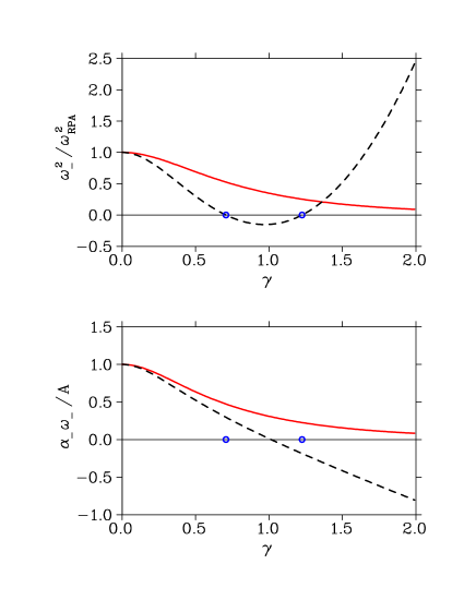
Figure 1: Upper panel: Dependence of the squared ERPA eigenvalue $\omega^{2}_{-}$ normalized to $\omega^{2}_{\mbox{\scriptsize RPA}}$ on the parameter $\gamma$ determining the strength of the coupling of the $ph$ pair with complex configuration. The values of $\omega^{2}_{-}$ are calculated by means of Eqs. (80)–(82) with $\beta=0.5$ and $\omega_{{}_{\mbox{\scriptsize$c$}}}=2$. Solid line represents the ERPA results obtained with the use of subtraction method ($\kappa=1$). The dashed line represents the results without subtraction ($\kappa=0$). The values of $(\bar{s}^{{}_{\mbox{\scriptsize RPA}}}_{\pm})^{1/2}$ are indicated by circles on the $\gamma$-axis. Lower panel: The same dependence for the product $\alpha_{{}_{\scriptstyle-}}\omega_{{}_{\scriptstyle-}}$ normalized to $\alpha_{{}_{\mbox{\scriptsize RPA}}}\omega_{{}_{\mbox{\scriptsize RPA}}}=A$ (see text for details).

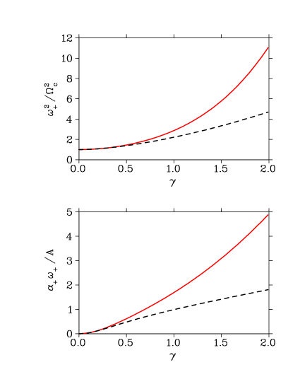
Figure 2: The same as Fig. 1 for $\omega^{2}_{+}$ normalized to $\Omega^{2}_{c}$ (upper panel) and $\alpha_{{}_{\scriptstyle+}}\omega_{{}_{\scriptstyle+}}$ (lower panel).

At $\kappa=0$ we have

• if $\gamma^{2}<\bar{s}^{{}_{\mbox{\scriptsize RPA}}}_{-}$, then $\,\omega^{\vphantom{*}}_{\pm}\,$ and $\,\alpha^{\vphantom{*}}_{\pm}\,$ are real and $\alpha^{\vphantom{*}}_{\pm}\omega^{\vphantom{*}}_{\pm}>0$;

• if $\bar{s}^{{}_{\mbox{\scriptsize RPA}}}_{-}<\gamma^{2}<\bar{s}^{{}_{\mbox{\scriptsize RPA}}}_{+}$, then $\omega^{\vphantom{*}}_{-}$ and $\alpha^{\vphantom{*}}_{-}$ are imaginary, $\omega^{\vphantom{*}}_{+}$ and $\alpha^{\vphantom{*}}_{+}$ are real and $\alpha^{\vphantom{*}}_{+}\omega^{\vphantom{*}}_{+}>0$;

• if $\gamma^{2}>\bar{s}^{{}_{\mbox{\scriptsize RPA}}}_{+}$, then $\omega^{\vphantom{*}}_{\pm}$ and $\alpha^{\vphantom{*}}_{\pm}$ are real, $\alpha^{\vphantom{*}}_{+}\omega^{\vphantom{*}}_{+}>0$, but $\alpha^{\vphantom{*}}_{-}\omega^{\vphantom{*}}_{-}<0$;

• if $\gamma^{2}=\bar{s}^{{}_{\mbox{\scriptsize RPA}}}_{\pm}$, then $\omega^{\vphantom{*}}_{+}$ and $\alpha^{\vphantom{*}}_{+}$ are real, $\alpha^{\vphantom{*}}_{+}\omega^{\vphantom{*}}_{+}>0$, $\omega^{\vphantom{*}}_{-}=0$, $\;\alpha^{\vphantom{*}}_{-}$ is indefinite.

These properties of the values $\omega^{\vphantom{*}}_{\pm}$ and $\alpha^{\vphantom{*}}_{\pm}$ do not depend on the value of the parameter $\omega^{\vphantom{*}}_{c}$ if $\Omega^{\vphantom{*}}_{c}>\omega^{\vphantom{*}}_{\mbox{\scriptsize RPA}}$.

Dependence of the values $\omega^{2}_{\pm}$ and $\alpha^{\vphantom{*}}_{\pm}\omega^{\vphantom{*}}_{\pm}$ on the parameter $\gamma$ at $\beta=0.5$ and $\omega_{{}_{\mbox{\scriptsize$c$}}}=2$ is shown in Figs. 1 and 2. Since $|\beta|<1$, the RPA stability condition (74) is fulfilled. We see that in this case the ERPA solutions are also stable and the eigenvalues of the ERPA residue matrices are non-negative at all $\gamma$ (and $\omega^{\vphantom{*}}_{\pm}>0$) if the subtraction method is used. In the ERPA without subtraction the lowest eigenvalue $\omega^{\vphantom{*}}_{-}$ becomes imaginary in the finite region of the values of $\gamma$ around the point $\gamma=1$. Outside of this region, the values of $\omega^{\vphantom{*}}_{-}$ at $\kappa=0$ are real, however at $\gamma^{2}>\gamma^{2}_{0}=1+\beta^{2}/(1+\omega^{\vphantom{*}}_{c})^{2}$ the product of $\omega^{\vphantom{*}}_{-}$ and the eigenvalue $\alpha^{\vphantom{*}}_{-}$ of the ERPA residue matrices $a^{\vphantom{*}}_{-,\,\pm}$ becomes negative. Using Eq. (85) we obtain that in this case the eigenvector with the positive eigenvalue $\omega^{\vphantom{*}}_{-}$ will have the negative norm. Therefore, the condition (65) is violated. In addition, in the region $\gamma^{2}>\bar{s}^{{}_{\mbox{\scriptsize RPA}}}_{+}$, where $\alpha^{\vphantom{*}}_{-}\omega^{\vphantom{*}}_{-}<0$, the matrices $a^{\vphantom{*}}_{-,\,\pm}\,$, though being Hermitian, become negative semidefinite at $\omega^{\vphantom{*}}_{-}>0$ (positive semidefinite at $\omega^{\vphantom{*}}_{-}<0$) that leads to the problem of the “negative transition probabilities” (or of the “negative energies”) as was explained in Sec. III.

From Eqs. (76) it follows that the subtraction effectively introduces additional repulsion into the matrix elements $A^{\vphantom{*}}_{ph,ph}$ and $A^{\vphantom{*}}_{hp,hp}$ of the matrix $\Omega^{{}_{\mbox{\scriptsize RPA}}}_{\vphantom{1}}$. As a result, $\omega^{2}_{-}(\kappa=1)>\omega^{2}_{-}(\kappa=0)$ at least at $\gamma^{2}<\bar{s}^{{}_{\mbox{\scriptsize RPA}}}_{-}$. Nevertheless, as can be seen from Fig. 1, $\omega^{2}_{-}<\omega^{2}_{\mbox{\scriptsize RPA}}$ for all $\gamma^{2}>0$ and $\kappa=1$ due to the attractive effect of the dynamic part of the interaction ${C}(\omega)$ at $\omega<\Omega^{\vphantom{*}}_{c}\,$.

VIII Conclusion

In the paper the problem of stability of solutions in the extended RPA (ERPA) theories is considered. The extension of the RPA implies enlarging the configuration space by taking into account more complex configurations in addition to the $1p1h$ states included in the RPA. The analysis of stability is based on the famous Thouless theorem proved in the case of the self-consistent RPA and on the response function formalism which enables one to study this problem in more detail. Two cases are considered: the ERPA with and without the subtraction method. This method was suggested previously to avoid double counting in the self-consistent ERPA approaches based on the density functional theory with phenomenologically fitted energy density functionals. Justification of the subtraction method is provided by the dielectric theorem which associates the static polarizability calculated within the self-consistent RPA with the exact inverse energy-weighted moment of the strength distribution including contributions of all configurations. The subtraction method ensures the equality of the RPA and of the ERPA static polarizabilities and, consequently, equality of the respective inverse energy-weighted moments.

It is proved that the stability matrix in the ERPA theories with subtraction is positive semidefinite if the RPA stability matrix possesses this property. This ensures stability of solutions of the ERPA eigenvalue equations, positiveness of the norms of the eigenvectors with positive eigenvalues, and non-negativeness of the respective transition probabilities. In the ERPA without subtraction these properties of the solutions are not guaranteed. In addition, it is shown that the subtraction method leads to the acceleration of the convergence in the ERPA though this problem is not generally resolved within the framework of this method.

The example of the schematic model is used to analyze dependence of the solutions of the ERPA equations on the effective parameter determining the strength of the coupling of a single particle-hole pair with a single complex configuration. It is demonstrated that, if the values of this parameter are sufficiently large, the ERPA without subtraction leads to the imaginary solutions of the respective eigenvalue equation and to the problem of the “negative transition probabilities” or of the “negative energies”. As in the general case, these problems do not arise when the subtraction method is applied.

References

(1)
P. Ring and P. Schuck,
The Nuclear Many-Body Problem
(Springer-Verlag, New York, 1980).
(2)
D. J. Thouless,
Nucl. Phys. 21, 225 (1960).
(3)
D. J. Thouless,
Nucl. Phys. 22, 78 (1961).
(4)
S. Drożdż, S. Nishizaki, J. Speth, and J. Wambach,
Phys. Rep. 197, 1 (1990).
(5)
H. Suhl and N. R. Werthamer,
Phys. Rev. 122, 359 (1961).
(6)
J. Sawicki,
Phys. Rev. 126, 2231 (1962).
(7)
C. Yannouleas, M. Dworzecka, and J. J. Griffin,
Nucl. Phys. A397, 239 (1983).
(8)
P. Papakonstantinou and R. Roth,
Phys. Lett. B671, 356 (2009).
(9)
P. Papakonstantinou and R. Roth,
Phys. Rev. C 81, 024317 (2010).
(10)
D. Gambacurta, M. Grasso, and F. Catara,
J. Phys. G: Nucl. Part. Phys. 38, 035103 (2011).
(11)
D. Gambacurta, M. Grasso, V. De Donno, G. Co’, and F. Catara,
Phys. Rev. C 86, 021304(R) (2012).
(12)
K. Moghrabi, M. Grasso, G. Colò, and N. Van Giai,
Phys. Rev. Lett. 105, 262501 (2010).
(13)
K. Moghrabi, M. Grasso, X. Roca-Maza, and G. Colò,
Phys. Rev. C 85, 044323 (2012).
(14)
V. V. Voronov, D. Karadjov, F. Catara, and A. P. Severyukhin,
Fiz. Elem. Chastits At. Yadra 31, 905 (2000)
[ Phys. Part. Nucl. 31, 452 (2000) ].
(15)
M. Tohyama and P. Schuck,
Eur. Phys. J. A 32, 139 (2007).
(16)
V. I. Tselyaev,
Yad. Fiz. 50, 1252 (1989)
[ Sov. J. Nucl. Phys. 50, 780 (1989) ].
(17)
S. P. Kamerdzhiev, G. Ya. Tertychny, and V. I. Tselyaev,
Fiz. Elem. Chastits At. Yadra 28, 333 (1997)
[ Phys. Part. Nucl. 28, 134 (1997) ].
(18)
S. Kamerdzhiev, J. Speth, and G. Tertychny,
Phys. Rep. 393, 1 (2004).
(19)
V. I. Tselyaev,
Phys. Rev. C 75, 024306 (2007).
(20)
E. V. Litvinova and V. I. Tselyaev,
Phys. Rev. C 75, 054318 (2007).
(21)
V. Tselyaev, J. Speth, S. Krewald, E. Litvinova,
S. Kamerdzhiev, N. Lyutorovich, A. Avdeenkov,
and F. Grümmer,
Phys. Rev. C 79, 034309 (2009).
(22)
A. Avdeenkov, S. Goriely, S. Kamerdzhiev,
and S. Krewald,
Phys. Rev. C 83, 064316 (2011).
(23)
E. Litvinova, P. Ring, and V. Tselyaev,
Phys. Rev. C 75, 064308 (2007).
(24)
E. Litvinova, P. Ring, and V. Tselyaev,
Phys. Rev. C 78, 014312 (2008).
(25)
E. Litvinova, P. Ring, and V. Tselyaev,
Phys. Rev. Lett. 105, 022502 (2010).
(26)
J. Speth, E. Werner, and W. Wild,
Phys. Rep. 33, 127 (1977).
(27)
J. Wambach,
in Proceedings of the International School on Nuclear Structure,
edited by V. G. Soloviev and Yu. P. Popov
(Joint Institute for Nuclear Research, Dubna, 1985), D4-85-851, p. 83.
(28)
G. Colò, N. Van Giai, P. F. Bortignon, and R. A. Broglia,
Phys. Rev. C 50, 1496 (1994).
(29)
V. G. Soloviev,
Theory of Atomic Nuclei: Quasiparticles and Phonons
(Institute of Physics, Philadelphia, 1992).
(30)
C. Mahaux, P. F. Bortignon, R. A. Broglia, and C. H. Dasso,
Phys. Rep. 120, 1 (1985).
(31)
H. Eschrig,
The Fundamentals of Density Functional Theory
(Edition am Gutenbergplatz, Leipzig, 2003).
(32)
M. Bender, P.-H. Heenen, and P.-G. Reinhard,
Rev. Mod. Phys. 75, 121 (2003).
(33)
J. E. Drut, R. J. Furnstahl, and L. Platter,
Progr. Part. Nucl. Phys. 64, 120 (2010).
(34)
O. Bohigas, A. M. Lane, and J. Martorell,
Phys. Rep. 51, 267 (1979).