Abstract

Compared to the other neutrino mixing angles $\theta_{13}$ is small. The solar mass splitting is about two orders smaller than the atmospheric splitting. We show that both could arise from a peturbation of a more symmetric structure. The perturbation also affects the solar mixing angle and can make alternate mixing patterns such as tribimaximal, bimaximal, or other variants equally viable. For real perturbations this can be accomplished only for normal mass ordering with the lightest neutrino mass less than 10^-2 eV. Both mass orderings can be accommodated by going over to complex perturbations if the lightest neutrino is heavier. The CP-phase in the lepton sector, fixed by $\theta_{13}$ and the lightest neutrino mass, distinguishes between different mixing models.

PACS No:  14.60.Pq
Key Words:  Neutrino mixing, $\theta_{13}$, Solar splitting, Perturbation

I Introduction

The recent measurement [1, 2] of a non-zero $\theta_{13}$ which is small compared to the other neutrino mixing angles has created a stir in the world of particle physics.

The Daya Bay collaboration after 127 days exposure has obtained for $\theta_{13}$ [1]

$$\sin^{2}2\theta_{13}=0.089\pm 0.010\;{\rm(stat)}\pm 0.005\;{\rm(syst)}\;\;{\rm(Daya~{}Bay)}$$ (1)

and from the RENO experiment with 229 days data [2] one has

$$\sin^{2}2\theta_{13}=0.113\pm 0.013\;{\rm(stat)}\pm 0.019\;{\rm(syst)}\;\;{\rm(RENO)}$$ (2)

The Double Chooz [3], MINOS [4], and T2K [5] experiments have also determined $\sin^{2}2\theta_{13}$, all consistent with the above but with larger uncertainties.

Earlier there already was in place a strong upper bound on this angle [6]. The measured value is close to this limit, leading to $\theta_{13}$ getting referred to occasionally as ‘large’. In terms of the three known mixing angles $\theta_{12}$, $\theta_{23}$, $\theta_{13}$ and a phase $\delta$ the Pontecorvo, Maki, Nakagawa, Sakata (PMNS) mixing matrix is usually parametrized as,

$$U=\pmatrix{c_{12}c_{13}&s_{12}c_{13}&s_{13}e^{-i\delta}\cr-s_{12}c_{23}-c_{12}s_{23}s_{13}e^{i\delta}&c_{12}c_{23}-s_{12}s_{23}s_{13}e^{i\delta}&s_{23}c_{13}\cr s_{12}s_{23}-c_{12}c_{23}s_{13}e^{i\delta}&-c_{12}s_{23}-s_{12}c_{23}s_{13}e^{i\delta}&c_{23}c_{13}}.$$ (3)

As it is now realized that in the lepton sector, as for the quarks, all three mixing angles are non-zero the door has been opened for CP-violation. Many alternative strategies are being considered to explore leptonic CP-violation as well as mixing and the future prospects are rich.

The other face of the neutrino sector is the mass spectrum. Indeed, from the several oscillation studies at accelerators and reactors complementing the solar and atmospheric neutrino measurements the mass splittings are now very well established though the absolute mass remains an unknown. From global fits the currently favoured values of the neutrino mixing parameters are [7, 8]:

$$\Delta m_{21}^{2} = (7.50^{+0.18}_{-0.19})\times 10^{-5}\,{\rm eV}^{2},\;\;\theta_{12}=(33.36^{+0.81}_{-0.78})^{\circ},$$

$$|\Delta m_{31}^{2}| = (2.473^{+0.070}_{-0.067})\times 10^{-3}\,{\rm eV}^{2},\;\;\theta_{23}=(40.0^{+2.1}_{-1.5}\oplus 50.4\pm 0.13)^{\circ}$$

$$\theta_{13} = (8.66^{+0.44}_{-0.46})^{\circ},\;\;\delta=(300^{+66}_{-138})^{\circ}\;\;.$$ (4)

Note that the atmospheric mixing angle, $\theta_{23}$, is no longer consistent with maximal mixing ($\theta_{23}=\pi/4$) at 1$\sigma$. There are best fit values in both the first and second octants; determining the $\theta_{23}$ octant is one of the priorities of future experiments. In this work to simplify the discussion and minimize parameters we will nonetheless take $\theta_{23}=\pi/4$. We comment on the effect of the small departure from maximality on the results. In the global fit $\theta_{12}$ is also large but not maximal while $\theta_{13}$ is the smallest of the three.

For the solar sector the splitting, $\Delta m_{21}^{2}$, is known in magnitude and sign while for the atmospheric neutrinos only the magnitude, $|\Delta m_{31}^{2}|$, has been determined, the sign remaining unknown. Thus two options are left open, the normal and the inverted ordering of the mass spectrum depending upon whether this undetermined sign is positive or negative. One noteworthy feature here is that the solar splitting is about two orders of magnitude smaller than the atmospheric splitting: $R_{\rm mass}=|\Delta m_{21}^{2}/\Delta m_{31}^{2}|=(3.03\pm 0.16)\times 10^{-2}$.

The non-zero value of $\theta_{13}$ close to its upper bound (‘large’) and yet small compared to the other mixing angles has attracted a great deal of attention from diverse angles. We list a sampling of this body of literature. For example, the role of $\mu-\tau$ symmetry [9], see-saw models [10], charged lepton contributions [11], and renormalization group effects [12] are among the avenues explored. A perturbative approach has been espoused in [13]. Other attempts have been based on diverse discrete symmetries [14, 15].

In this work we seek to address the following question: Is it possible that at some level the small quantities, the ratio $R_{\rm mass}$ and $\theta_{13}$, are vanishing and that a single perturbation induces the observed non-zero values for both? The answer is in the affirmative. To our knowledge, this result was pointed out for the first time through a specific example in [17]. Here, we make an exhaustive analysis and show that the existence (or not) of a viable solution depends on two factors: the ordering of the neutrino masses and the mass of the lightest neutrino, $m_{0}$. For normal ordering, for a large choice of parameters the requirements can be met. The perturbation can be real or complex. In the latter case, CP-violation is present. The inverted ordering is less favoured if the perturbation is real. In this case one would have to admit significant differences in the sizes of the matrix elements of the perturbation to get satisfactory solutions.

Our paper is structured as follows. In the next section we set up the framework for our discussion and list some of the commonly considered neutrino mixing schemes, e.g., tribimaximal mixing. In the following section we elaborate on the degenerate perturbative mechanism which we will adopt. Next we discuss to what extent the global fits of the mixing parameters constrain the choice of the perturbation. Our main results are presented in the following section where we show the allowed ranges of the perturbation matrix for the two mass orderings and the predictions for CP-violation. We then briefly indicate how the perturbation can arise from a mass model. We end with the conclusions and discussions.

II Neutrino mass and mixing scenarios

We restrict ourselves to the case of three flavours of neutrinos. We also work in a basis where the charged lepton mass matrix is diagonal. In this basis the entire lepton mixing resides in the neutrino mass matrix.

Our starting point will be the unperturbed Majorana neutrino mass matrix, $M^{0}$, which is always symmetric. We choose a form such that the solar splitting is absent; i.e., in the mass basis one has

$$M^{0}_{mass}=diag(m^{(0)}_{1},m^{(0)}_{1},m^{(0)}_{3}).$$ (5)

For a specific mass ordering, the lightest neutrino mass, $m_{0}$, determines $m^{(0)}_{1}$ and $m^{(0)}_{3}$. It is useful to define $m^{\pm}=(m^{(0)}_{3}\pm m^{(0)}_{1})$. $m^{-}$ is positive (negative) for normal (inverted) mass ordering.

In the flavour basis the mass matrix becomes:

$$M^{0}_{flavour}={U^{0}}\pmatrix{m^{(0)}_{1}&&\cr&m^{(0)}_{1}&\cr&&m^{(0)}_{3}}{U^{0}}^{T}\;,$$ (6)

where $U^{0}$ is the lowest order leptonic mixing matrix. The columns of $U^{0}$ are the unperturbed flavour eigenstates. Neutrino mass models lead to predictions for $U^{0}$ of which three often-discussed variants are the tribimaximal (TBM), bimaximal (BM), and the ‘golden ratio’ (GR) forms. Each of these imply $\theta_{13}=0$ and $\theta_{23}=\pi/4$. They differ only in $\theta_{12}$. We will consider them in turn along with a further option where there is no solar mixing to start with.

Our goal is to check whether in each case a perturbation mass matrix, $M^{\prime}$ (also symmetric), can be identified which will add corrections to $M^{0}$ and $U^{0}$ leading to mass splittings and mixing angles in agreement with observations, in particular that the correct $\Delta m_{21}^{2}$ and $\theta_{13}$ are realized.

II.1 General parametrization

In general as long as $\theta_{13}=0$ and the atmospheric mixing is maximal ($\theta_{23}=\pi/4$) the leptonic mixing matrix can be parametrized as:

$$U^{0}=\pmatrix{b&a&0\cr-a/\sqrt{2}&b/\sqrt{2}&\sqrt{1\over 2}\cr a/\sqrt{2}&-b/\sqrt{2}&\sqrt{1\over 2}},$$ (7)

with

$$a^{2}+b^{2}=1.$$ (8)

For the above $U^{0}$ the solar mixing angle is given by $\tan\theta^{0}_{12}=a/b$. The experimentally determined range of $\theta_{12}$ in Eq. (4) corresponds to $0.539\leq a\leq 0.561$ at 1$\sigma$.

II.2 Tribimaximal mixing

The preferred values of the mixing angles are reasonably close to a mixing matrix of tribimaximal form [20],

$$U^{0}=\pmatrix{\sqrt{2\over 3}&\sqrt{1\over 3}&0\cr-\sqrt{1\over 6}&\sqrt{1\over 3}&\sqrt{1\over 2}\cr\sqrt{1\over 6}&-\sqrt{1\over 3}&\sqrt{1\over 2}},$$ (9)

which predicts the third mixing angle $\theta_{13}$ to be exactly vanishing.

II.3 Bimaximal mixing

For bimaximal mixing the matrix is [21],

$$U^{0}=\pmatrix{\sqrt{1\over 2}&\sqrt{1\over 2}&0\cr-{1\over 2}&\frac{1}{2}&\sqrt{1\over 2}\cr{1\over 2}&-{1\over 2}&\sqrt{1\over 2}},$$ (10)

which also has a vanishing $\theta_{13}$.

II.4 Golden ratio mixing

A third form of the mixing matrix also appearing in the literature involves the golden ratio $\phi=(1+\sqrt{5})/2$ [22],

$$U^{0}=\pmatrix{\sqrt{\phi\over\sqrt{5}}&\sqrt{1\over\sqrt{5}\phi}&0\cr-{1\over\sqrt{2}}\sqrt{\frac{1}{\sqrt{5}\phi}}&{1\over\sqrt{2}}\sqrt{\frac{\phi}{\sqrt{5}}}&\sqrt{1\over 2}\cr{1\over\sqrt{2}}\sqrt{\frac{1}{\sqrt{5}\phi}}&-{1\over\sqrt{2}}\sqrt{\frac{\phi}{\sqrt{5}}}&\sqrt{1\over 2}},$$ (11)

which too gives $\theta_{13}=0$.

II.5 No solar mixing

Finally, we also examine the possibility that the unperturbed mixing matrix has $a$ = 0. This would imply one degenerate state decoupled and the other maximally mixed to the third (nondegenerate) state. For this choice $\theta_{12}^{0}$ = 0. Another case with one decoupled degenerate state is $b$ = 0 for which $\theta_{12}^{0}=\pi/2$. These cases give identical physics results.

Mixing	Global fit 1$\sigma$		Global fit 3$\sigma$		TBM	BM	GR
parameter	$a_{min}$	$a_{max}$	$a_{min}$	$a_{max}$
$a$	0.539	0.561	0.515	0.585	0.577	0.707	0.526

Table 1: The limits on the mixing parameter $a\equiv\sin\theta^{0}_{12}$ as obtained from the global fit. The values of $a$ for the TBM, BM, and GR forms are also shown.

In Table 1 we list the allowed range of $a$ from the global fit and its values in the TBM, BM, and the GR models. As noted, the unperturbed matrix, $M^{0}$, is such that the solar splitting is absent and two eigenvalues are degenerate. Due to this degeneracy the two corresponding eigenstates are non-unique. The perturbation, $M^{\prime}$, which splits the degeneracy determines the actual eigenstates which will be rotated with respect to the first two columns of $U^{0}$ – Eq. (7) – by an angle $\zeta$ also determined by $M^{\prime}$. Therefore, on inclusion of the perturbation we have a resultant solar mixing angle given by $\theta_{12}=\theta^{0}_{12}+\zeta$.

III Perturbation Strategy

We will work in the mass basis unless explicitly mentioned otherwise. Our discussion will involve only first order perturbative corrections. The perturbation $M^{\prime}$ is a $(3\times 3)$ symmetric matrix which could be real or complex. These two cases will be treated sequentially. The former provides a good starting point for the latter.

After removing an irrelevant constant part the perturbation, $M^{\prime}$, can be written as:

$$M^{\prime}=m^{+}\pmatrix{0&\gamma&\xi\cr\gamma&\alpha&\eta\cr\xi&\eta&\beta}\;\;.$$ (12)

III.1 Real Perturbation

In this case all entries in the matrix $M^{\prime}$ are real. For perturbation theory to be acceptable the dimensionless entities $\alpha,\beta,\gamma,\xi,\eta$ should be small compared to unity. Taken together with the unperturbed $M^{0}$ – Eq. (5) – at lowest order the perturbation will induce the solar oscillation parameters through $\alpha$ and $\gamma$; $\theta_{13}$ will be determined by $\xi$ and $\eta$; while $\beta$ will result in a small correction to $m^{(0)}_{3}$.

III.2 Complex Perturbation

If $M^{\prime}$ is complex symmetric then it is not hermitian. In such an event one takes the hermitian combination $(M^{0}+M^{\prime})^{\dagger}(M^{0}+M^{\prime})$ and considers $M^{0\dagger}M^{0}$ as the unperturbed term and $(M^{0\dagger}M^{\prime}+M^{\prime\dagger}M^{0})$ as the lowest order perturbation. The unperturbed eigenvalues will now be $(m^{(0)}_{i})^{2}$ and the perturbation matrix

$$(M^{0\dagger}M^{\prime}+M^{\prime\dagger}M^{0})=m^{+}\pmatrix{0&2m^{(0)}_{1}{\rm Re}(\gamma)&m^{+}{\rm Re}(\xi)-i~{}m^{-}{\rm Im}(\xi)\cr 2m^{(0)}_{1}{\rm Re}(\gamma)&2m^{(0)}_{1}{\rm Re}(\alpha)&m^{+}{\rm Re}(\eta)-i~{}m^{-}{\rm Im}(\eta)\cr m^{+}{\rm Re}(\xi)+i~{}m^{-}{\rm Im}(\xi)&m^{+}{\rm Re}(\eta)+i~{}m^{-}{\rm Im}(\eta)&2m^{(0)}_{3}{\rm Re}(\beta)}\;\;.$$ (13)

The imaginary parts of $\alpha$, $\beta$, and $\gamma$ do not appear in Eq. (13). However, they do contribute at higher order via the $M^{\prime\dagger}M^{\prime}$ term.

IV Relating elements of $M^{\prime}$ to the data

We look for solutions which are consistent with the global neutrino parameter fits up to 1$\sigma$. In particular, the solar mass splitting and $\theta_{13}$ must both emerge from the perturbation. We discuss these aspects now.

IV.1 The solar mixing angle

To lowest order, the solar mass splitting is obtained via the $(2\times 2)$ submatrix of the perturbation, $M^{\prime}$, in the space of the first two generations. For real $M^{\prime}$ in terms of $r=\gamma/\alpha$ from eq. (12) this submatrix is:

$$M^{\prime}_{(2\times 2)}=m^{+}\alpha\pmatrix{0&r\cr r&1}\;{\rm for~{}Real}~{}M^{\prime}\;.\;$$ (14)

If $M^{\prime}$ is complex then $r={\rm Re}(\gamma)/{\rm Re}(\alpha)$ and

$$(M^{0\dagger}M^{\prime}+M^{\prime\dagger}M^{0})_{(2\times 2)}=2m^{+}m^{(0)}_{1}{\rm Re}(\alpha)\pmatrix{0&r\cr r&1}\;{\rm for~{}Complex}~{}M^{\prime}\;\;.$$ (15)

If $r=0$ then $M^{\prime}$ will produce a mass splitting but will not change the solar mixing. For $r$ non-zero the eigenstates are rotated from those in $U^{0}$ through an angle $\zeta$ given by

$$\zeta=\frac{1}{2}\tan^{-1}(2r)\;,$$ (16)

independent of the prefactor of the matrix. As noted, the tribimaximal, bimaximal and golden ratio mixing models do not satisfy the currently measured value of $\theta_{12}$ within 1$\sigma$. Therefore for these cases we choose $r\neq 0$ in such a manner that when the mass degeneracy is removed the mixing angle is tweaked to within the allowed range. In Table 2 we show the ranges of $r$ for each of the three models that result in $\theta_{12}$ values consistent with observations. It is noteworthy that $r$ is small in every case (but for the $\theta_{12}^{0}=0$ alternative). Since it is a ratio of two elements of the perturbation matrix it could, in principle, be ${\cal O}$(1). The smallness can be traced to the fact that as $r\rightarrow 0$ the mass matrix in the flavour basis exhibits a $Z_{2}\times Z_{2}$ symmetry of the unperturbed model generated by:

$$U_{1}=1-2~{}\pmatrix{a^{2}&ab/\sqrt{2}&-ab/\sqrt{2}\cr ab/\sqrt{2}&b^{2}/2&-b^{2}/2\cr-ab/\sqrt{2}&-b^{2}/2&b^{2}/2}\;\;{\rm and}\;\;U_{2}=1-2~{}\pmatrix{b^{2}&-ab/\sqrt{2}&ab/\sqrt{2}\cr-ab/\sqrt{2}&a^{2}/2&-a^{2}/2\cr ab/\sqrt{2}&-a^{2}/2&a^{2}/2}\;.$$ (17)

Parameter	TBM		BM		GR		$\theta_{12}^{0}=0$
	$r_{min}$	$r_{max}$	$r_{min}$	$r_{max}$	$r_{min}$	$r_{max}$	$r_{min}$	$r_{max}$
$r~{}(\times 10^{2})$	-4.59	-1.95	-23.1	-19.9	1.54	4.18	108	125

Table 2: The range of the off-diagonal entry, $r=\gamma/\alpha$, in the 2$\times$2 submatrix of the perturbation (see Eqs. (14, 15)) for the TBM, BM, and GR alternatives that produces a $\theta_{12}$ consistent with the global fits at 1$\sigma$. The $\theta_{12}^{0}=0$ alternative is also noted.

Before closing this subsection it is worth noting that to lowest order in degenerate perturbation theory the first two eigenstates are:

$$|\psi_{1}\rangle=\cos\zeta\left[\pmatrix{b\cr-a/\sqrt{2}\cr a/\sqrt{2}}-\bar{\xi}\pmatrix{0\cr 1/\sqrt{2}\cr 1/\sqrt{2}}\right]-\sin\zeta\left[\pmatrix{a\cr b/\sqrt{2}\cr-b/\sqrt{2}}-\bar{\eta}\pmatrix{0\cr 1/\sqrt{2}\cr 1/\sqrt{2}}\right]\;,\;$$ (18)

$$|\psi_{2}\rangle=\sin\zeta\left[\pmatrix{b\cr-a/\sqrt{2}\cr a/\sqrt{2}}-\bar{\xi}\pmatrix{0\cr 1/\sqrt{2}\cr 1/\sqrt{2}}\right]+\cos\zeta\left[\pmatrix{a\cr b/\sqrt{2}\cr-b/\sqrt{2}}-\bar{\eta}\pmatrix{0\cr 1/\sqrt{2}\cr 1/\sqrt{2}}\right]\;,\;$$ (19)

with $\zeta$ defined in Eq. (16) and

$$\bar{\xi}=\left(\frac{m^{+}}{m^{-}}\right)\xi,\;\;\bar{\eta}=\left(\frac{m^{+}}{m^{-}}\right)\eta\;{\rm for~{}Real}~{}M^{\prime},$$ (20)

and

$$\bar{\xi}=\left(\frac{m^{+}}{m^{-}}\right){\rm Re}(\xi)+i~{}{\rm Im}(\xi),\;\;\bar{\eta}=\left(\frac{m^{+}}{m^{-}}\right){\rm Re}(\eta)+i~{}{\rm Im}(\eta)\;{\rm for~{}Complex}~{}M^{\prime}\;.$$ (21)

IV.2 The solar mass splitting

The solar mass splitting is determined by the eigenvalues of the submatrix in Eqs. (14) and (15).

For real $M^{\prime}$ the first order corrections to the degenerate eigenvalues are:

$$m^{(1)}_{2,1}=m^{+}~{}\frac{\alpha}{2}\left[1\pm\sqrt{1+4r^{2}}\right]\;.$$ (22)

Identifying the heavier eigenvalue with $m_{2}$, as required by the solar data, one has:

$$m^{2}_{2}-m^{2}_{1}=2m^{+}m^{(0)}_{1}\alpha\sqrt{1+4r^{2}}\;.$$ (23)

Up to small perturbative corrections $m^{+}m^{-}$ gives the atmospheric mass splitting. Hence:

$$R_{\rm mass}=|(m^{2}_{2}-m^{2}_{1})/(m^{2}_{3}-m^{2}_{1})|=2\frac{m^{(0)}_{1}}{|m^{-}|}~{}\alpha\sqrt{1+4r^{2}}\;.$$ (24)

For complex $M^{\prime}$ the corrections are to the squared masses and one directly obtains Eqs. (23) and (24) but for the replacement $\alpha\rightarrow{\rm Re}(\alpha)$.

We will return to this equation when we discuss numerical estimates of the element $\alpha$.

IV.3 Generating $\theta_{13}\neq 0$

Using first order degenerate perturbation theory the corrected wave-function $|\psi_{3}\rangle$ is given by:

$$|\psi_{3}\rangle=\pmatrix{0\cr 1/\sqrt{2}\cr 1/\sqrt{2}}+\bar{\xi}^{*}\pmatrix{b\cr-a/\sqrt{2}\cr a/\sqrt{2}}+\bar{\eta}^{*}\pmatrix{a\cr b/\sqrt{2}\cr-b/\sqrt{2}}\;.$$ (25)

To minimize the number of free parameters we will restrict ourselves to only those perturbations which leave the atmospheric mixing angle $\theta_{23}$ fixed at the maximal value of $\pi/4$. This gives the relationship:

$$\left(\frac{\bar{\xi}}{\bar{\eta}}\right)^{*}=\frac{b}{a}$$ (26)

Since $a$ and $b$ are real Eq. (26) implies that $\bar{\xi}$ and $\bar{\eta}$ and hence $\xi$ and $\eta$ have the same phase. Comparing with Eq. (3) one then has:

$$\sin\theta_{13}~{}e^{-i\delta}=\left[b~{}\bar{\xi}^{*}+a~{}\bar{\eta}^{*}\right]=\frac{\bar{\xi}^{*}}{b}\;,$$ (27)

where we have used $(a^{2}+b^{2})=1$.

For real $M^{\prime}$ one has $\delta=0$. Hence, from Eq. (20)

$$\xi=\left(\frac{m^{-}}{m^{+}}\right)b\sin\theta_{13}\;.$$ (28)

In the next section, these formulae will be used to relate $M^{\prime}$ to the neutrino masses and mixings.

V Results

We now have all the ingredients in place to determine the full perturbation matrix and extract the consequences. Once the neutrino mass ordering is chosen and the lightest neutrino mass, $m_{0}$, specified, the unperturbed mass spectrum is fixed. The matrix element $\alpha$ is determined from the solar splitting through Eq. (24). The element $\beta$ makes a small contribution (a few per cent) to the atmospheric neutrino splitting and does not affect the physics at hand and so will not be pursued any further in this section. $\gamma$ is fixed by the ratio $r$ (see Table 2). Finally, $\xi$ and $\eta$ are determined through Eqs. (26) - (28). The question to be examined, for each of the popular mixing patterns for both mass ordering options, is for what range of $m_{0}$ are these matrix elements of acceptable magnitude as a perturbation?

V.1 Real perturbation

First we consider $M^{\prime}$ real which amounts to $\delta$ = 0 and CP-conservation. In this case one can determine the dependence of $\alpha$ on $m_{0}$ using Eq. (24). Since $\xi$ and $\eta$ are proportional to each other – see Eq. (26) – presenting any one of them is adequate. Here we present $\xi$ (which is larger than (equal to) $\eta$ for the TBM and GR (BM) mixing models) as a function of $m_{0}$ as obtained from Eq. (28).

V.1.1 Normal mass ordering

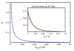
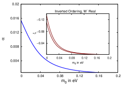
Figure 1: $\alpha$ and $\xi$ (inset) as a function of the lightest neutrino mass $m_{0}$ for real $M^{\prime}$. The left (right) panel is for normal (inverted) mass ordering. In the insets the region between the two curves is allowed when $\theta_{13}$ is varied over its 1$\sigma$ range. The results for $\xi~{}(\propto b)$ are for tribimaximal mixing ($b_{TBM}=\sqrt{\frac{2}{3}}\sim 0.816$). The corresponding plots for bimaximal ($b_{BM}=\frac{1}{\sqrt{2}}=0.707$), ‘golden ratio’ mixing ($b_{GR}=\sqrt{\frac{\phi}{\sqrt{5}}}\sim 0.851$), and the $\theta_{12}^{0}=0$ model ($b=1$) can be obtained by scaling.

The results for normal ordering are in the left panel of Fig. 1. $\alpha$ is presented as a function of the lightest neutrino mass $m_{0}$. We have shown the case for $r$ = 0. We have verified that using the small values of $r$ required to fit the solar mixing angle $\theta_{12}$ for the popular models – see Table 2 – in Eq. (24) causes no perceptible change in $\alpha$. $r$ is larger for the $\theta_{12}^{0}=0$ model and this effectively reduces $\alpha$ by a factor of around 2. As expected, $\alpha$ diverges as $m_{0}$ tends to zero.

In the inset we show $\xi$ as a function of $m_{0}$ for the 1$\sigma$ limits of $\theta_{13}$. In these plots $b=\sqrt{\frac{2}{3}}$ corresponding to tribimaximal mixing. For the other commonly considered alternatives – bimaximal ($b=\frac{1}{\sqrt{2}}$) and ‘golden ratio’ ($b=\sqrt{\frac{\phi}{\sqrt{5}}}$) mixing – the ordinate should be scaled appropriately. For the $\theta_{12}^{0}=0$ model one must use $b=1$.

At this stage one can identify a favoured region of $m_{0}$ by requiring that the elements of $M^{\prime}$ – such as $\xi$ and $\alpha$ – should be of similar order. For this purpose, we plot in Fig. 2 the ratio $|\xi/\alpha|$ as a function of $m_{0}$ (green solid curves). For easy identification we have shown where this ratio corresponds to the values 3 and $\frac{1}{3}$ (dot-dashed black lines), two limits separated by an order of magnitude. Notice that for normal ordering the ratio is within the above limits only if $2.3\times 10^{-3}~{}{\rm eV}\leq m_{0}\leq 3.7\times 10^{-2}~{}{\rm eV}$. If from other experiments a larger value of $m_{0}$ is determined then that could be an indication that $M^{\prime}$ must be complex, as we discuss in the following section. We remind the reader that these curves are for tribimaximal mixing. For the bimaximal (‘Golden ratio’) case the $\xi/\alpha$ curves will be lowered (raised) by about 13.35 % (4.28 %). For the $\theta_{12}^{0}=0$ model $\alpha$ is reduced by a factor of about 2 while $\xi$ is enhanced by 25%. As an upshot $\xi/\alpha$ is 2.5 times larger, squeezing allowed $m_{0}$ to smaller values.

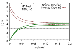
Figure 2: The ratio $|\xi/\alpha|$ is plotted as function of the lightest neutrino mass $m_{0}$ for both mass orderings when the perturbation $M^{\prime}$ is real. The area between the two curves of the same type is allowed when $\theta_{13}$ is varied over its 1$\sigma$ range. Also indicated are the values $1\over 3$ and 3 for $|\xi/\alpha|$ – black dot-dashed lines.

V.1.2 Inverted mass ordering

The results for inverted ordering appear in the right panel of Fig. 1. As before, $\alpha$ as a function of $m_{0}$ is shown for $r$ = 0 while $\xi$ for the 1$\sigma$ range of $\theta_{13}$ is given in the inset. As for normal ordering, inclusion in Eq. (24) of the small values of $r$ required to achieve the best-fit $\theta_{12}$ in the TBM, BM, and GR models causes essentially no change in $\alpha$. For the $\theta_{12}^{0}=0$ model $\alpha$ is roughly halved. Once again, we have used the TBM value $b=\sqrt{\frac{2}{3}}$ for the calculation of $\xi$. In this case $\xi$ turns out to be negative. The two curves in the $\xi$ panel correspond to the 1$\sigma$ limits of $\theta_{13}$.

The noteworthy difference from normal ordering is that $\alpha$ is about an order of magnitude smaller than $|\xi|$ for most of the range of $m_{0}$. The brown dotted curves in Fig. 2 depict the ratio $|\xi/\alpha|$ for inverted ordering. It is seen that they lie outside the range of 1/3 to 3 for all $m_{0}$ considered. Thus the inverted ordering case would be a less favoured alternative for this picture if the perturbation is real.

V.2 Complex perturbation

We now turn to the case of complex $M^{\prime}$. If perturbation theory is to be meaningful then we should expect the magnitudes of the different dimensionless complex elements of $M^{\prime}$ to be small compared to unity. Barring fine tuning, they should also be of roughly similar order. Below, we take a conservative stand and set:

$$\alpha=\epsilon\exp(i\phi_{\alpha}),~{}\gamma=\epsilon\exp(i\phi_{\gamma}),~{}\xi=\epsilon\exp(i\phi_{\xi}).$$ (29)

The dimensionless quantity $\epsilon$ sets the scale of the perturbation. The phases $\phi_{\alpha},\phi_{\gamma}$ and $\phi_{\xi}$ are left arbitrary.

It is seen from Eq. (21) that

$$\tan\delta=\tan\phi_{\bar{\xi}}=\left(\frac{m^{-}}{m^{+}}\right)\tan{\phi_{\xi}}$$ (30)

where $\phi_{\bar{\xi}}$ is the phase of $\bar{\xi}$.

As we elaborate in the following, the phase freedom still leaves room for some flexibility. In particular, we will mostly focus on those ranges of $m_{0}$ which are disfavoured for real $M^{\prime}$ as they do not satisfy the chosen criterion $3\geq|\xi/\alpha|\geq 1/3$. We show that such $m_{0}$ are accommodated for complex $M^{\prime}$.

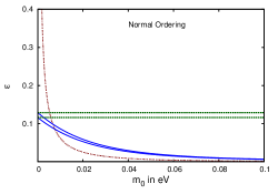
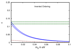
Figure 3: The limits on the scale of the perturbation, $\epsilon$, for normal (left panel) and inverted (right panel) mass orderings as a function of the lightest neutrino mass $m_{0}$. The upper (lower) limits from Eq. (31) for tribimaximal mixing are the green dashed (blue solid) curves. The region between the curves of the same type correspond to $\theta_{13}$ values in the 1$\sigma$ range. The dotted maroon curves are the lower limits from Eq. (32). Here $r$ = 0 has been taken.

The choice of $\epsilon$ is not entirely arbitrary. In particular, Eq. (21) implies:

$$\left|\frac{m^{+}}{m^{-}}\right|~{}\epsilon~{}\geq~{}|\bar{\xi}|~{}\geq~{}\epsilon\;\;.$$ (31)

These limits are presented in the left (right) panel of Fig. 3 for the normal (inverted) mass ordering. The upper and lower limits on $\epsilon$ are shown as the green dashed and blue solid curves. The two curves of each type show how the limit changes as $\theta_{13}$ is allowed to vary over its 1$\sigma$ range. Tribimaximal mixing has been assumed for these plots.

In addition, from Eq. (24) one has

$$\epsilon\geq\left|\frac{m^{-}}{2m^{(0)}_{1}\sqrt{1+4r^{2}}}\right|R_{\rm mass}\;.$$ (32)

The lower limit from this equation is indicated by the dotted maroon curves in the two panels of Fig. 3. This limit is independent of both (a) the choice of $\theta_{13}$ and (b) whether the mixing is of the tribimaximal, bimaximal, or Golden ratio nature. We have checked that the dependence on $r$ is insignificant for the physics calculations. It can be seen from the left (right) panel of Fig. 3 that for the normal ordering (inverted ordering) for most values of $m_{0}$ (for all values $m_{0}$) the lower limit on $\epsilon$ from $\bar{\xi}$ is more restrictive. Guided by these results, in the following we choose $\epsilon$ = 0.1, 0.05, and 0.025.

V.2.1 Normal mass ordering

From Fig. 2 it is seen that for real $M^{\prime}$ and normal mass ordering $|\xi/\alpha|$ is outside the chosen range for $m_{0}\geq 0.04$ eV. If $M^{\prime}$ is complex, $\alpha$ in eq. (24) is replaced by ${\rm Re}(\alpha)$. Demanding that the solar splitting is correctly obtained fixes $\phi_{\alpha}$ when $\epsilon$ is chosen. The results are shown in the left panel of Fig. 4 for $\epsilon$ = 0.1, 0.05, and 0.025.

One can conclude from Fig. 1 that as $m_{0}$ increases ${\rm Re}(\alpha)$ approaches zero. This is reflected in Fig. 4 (left panel) where $\phi_{\alpha}$ tends to $\pi/2$ asymptotically for all choices of $\epsilon$. For a particular $\epsilon$ the lightest neutrino mass $m_{0}$ has a lower limit set by Eq. (31) where the curves have been terminated. The corresponding $\phi_{\alpha}$ can be read off from Fig. 3 – $\cos\phi_{\alpha}$ is the ratio of the value of the dot-dashed maroon curve to that of the blue solid curve at this $m_{0}$. For these plots we have taken $r=0$; the small corrections ${\cal O}(r^{2})$ for the TBM, BM, and GR models are insignificant. In the $\theta_{12}^{0}=0$ model ${\rm Re}(\alpha)$ is reduced to about half and so $\phi_{\alpha}$ tends closer to $\pi/2$. One should bear in mind that we have used the central value of $R_{\rm mass}$ which has a $\pm 5$% uncertainty.

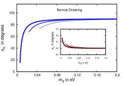
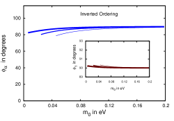
Figure 4: $\phi_{\alpha}$ ($\phi_{\gamma}$) for a complex $M^{\prime}$ is shown as a function of $m_{0}$ for normal mass ordering in the left panel (left panel inset) for three values of $\epsilon$: in decreasing order of line-thickness 0.1, 0.05 and 0.025. In the right panel the same plots are displayed for inverted mass ordering.

As presented in Table 2, in the TBM, BM, and GR models the ratio $r={\rm Re}(\gamma)/{\rm Re}(\alpha)=\cos\phi_{\gamma}/\cos\phi_{\alpha}$ is tightly constrained from the solar mixing angle $\theta_{12}$. Thus $\phi_{\gamma}$ also tends to $\pi/2$ as $m_{0}$ increases and since $r$ is small it does so faster than $\phi_{\alpha}$. This can be seen from the inset in Fig. 4.

$\delta$ is not a free parameter in this model. Rather, picking a value for $\theta_{13}$ amounts to fixing $|\bar{\xi}|$ from Eq. (27). Now, by choice $|\xi|=\epsilon$, hence from Eq. (21) one can get $\phi_{\xi}$. This in turn determines the phase of $\bar{\xi}$ which equals $\delta$. The results so obtained are presented in the left panel of Fig. 5 for the TBM (red solid), BM (violet dashed), and GR (green dot-dashed) models for $\epsilon=0.1$. The brown dotted curves are for $a=0,b=1$. For each model the two curves correspond to the 1$\sigma$ upper and lower limits of $\theta_{13}$. It is worthwhile to point out that the procedure for extracting $\delta$ using $|\bar{\xi}|$ leaves a two-fold uncertainty $\delta\leftrightarrow\pi+\delta$. Keeping this in mind we have shown $\delta$ in the first quadrant in Fig. 5 even though the 1$\sigma$ range of the global fit – Eq. (4) – would prefer the partner $\pi+\delta$ solution.

In the right panel of Fig. 5 we restrict to the case of tribimaximal mixing and show the dependence of $\delta$ on the scale of perturbation $\epsilon$. The conclusion that can be drawn from these panels is that $\delta$ is largely independent of the lightest neutrino mass and varies over a limited region as $\theta_{13}$ covers its 1$\sigma$ range or $\epsilon$ is varied.

A reparametrization invariant measure of CP-violation is the Jarlskog parameter, $J$ [23]. For arbitrary mixing it turns out to be

$$J={\rm Im}[U_{e1}U_{\mu 2}U^{*}_{e2}U^{*}_{\mu 1}]=\frac{1}{4b}\left[(b^{2}-a^{2})\sin 2\zeta+2ab\cos 2\zeta\right]Im(\bar{\xi})\;,$$ (33)

where in the last step only the lowest order perturbation effect is retained. In the inset of the right panel of Fig 5 we show this CP-violation measure as a function of $m_{0}$. Note that $J$ changes sign under $\delta\rightarrow\pi+\delta$. We remark at this stage that for the $b=0$ case $J$ = 0.

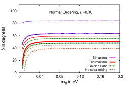
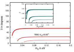
Figure 5: In the left panel $\delta$ for different models is plotted for the 1$\sigma$ limiting values of $\theta_{13}$, namely, $9.1^{\circ}$ (thick curves) and $8.2^{\circ}$ (thin curves). $\epsilon$ has been taken to be 0.1. The right panel is for the TBM model. Three values of $\epsilon$ are chosen – in decreasing order of thickness $\epsilon$ = 0.1, 0.05, 0.025 – and $\theta_{13}$ is taken at the best-fit value. In the inset is shown the Jarlskog parameter $J$ for the chosen $\epsilon$ and the 1$\sigma$ limits of $\theta_{13}$. Both panels are for normal mass ordering. For inverted ordering $\delta\rightarrow(\pi-\delta)$ and $J$ is unchanged.

V.2.2 Inverted mass ordering

The analysis procedure for inverted mass ordering is essentially the same. In the right-panel of Fig. 4 we show $\phi_{\alpha}$ (with $\phi_{\gamma}$ in the inset) as a function of $m_{0}$. The difference from normal ordering arises due to the appearance of $m_{1}^{(0)}$ in Eq. (24) which is larger in this case. Hence, $\phi_{\alpha}$ and $\phi_{\gamma}$ remain closer to $\pi/2$ for all $m_{0}$. The determination of $\delta$ using Eqs. (27) and (30) on the other hand involves only $m^{\pm}$ and not $m_{i}^{(0)}$. Consequently, it can be seen from Eq. (30) that for any $m_{0}$ the CP-phase in the inverted and normal mass orderings are simply related by $\delta\leftrightarrow(\pi-\delta)$. $J$ remains unchanged. So, $\delta$ and $J$ for the inverted mass ordering can be read off from Fig. 5.

VI Mass models

The discussion thus far has not been tied to any specific model for neutrino masses. We restrict ourselves to just a few remarks here. The perturbation matrix in the flavour basis corresponding to the general form of the mixing matrix in Eq. (7) is:

$$M^{\prime}_{flavour}=m^{+}~{}\pmatrix{a^{2}\alpha&\chi&-\sqrt{2}ab\alpha+\chi\cr\chi&(b^{2}\alpha+\beta)/2&(-b^{2}\alpha+\beta)/2\cr-\sqrt{2}ab\alpha+\chi&(-b^{2}\alpha+\beta)/2&(b^{2}\alpha+\beta)/2}$$ (34)

where use has been made of Eq. (26) and we have set $\chi=(ab\alpha+b\xi+a\eta)/\sqrt{2}$.

Attempting to relate the above matrix in its general form to the popular mass models will take us beyond the scope of this paper. Rather, we indicate here a limit when it can arise from a Zee-type model [24]. The required condition is:

$$\beta=\alpha(2-3b^{2})$$ (35)

It is seen using Eq. (8) that for this choice the diagonal elements of $M^{\prime}_{flavour}$ become equal and can be subsumed in the unperturbed matrix. The remaining terms can be obtained from a Zee-type model. In these models $(M^{\prime}_{flavour})_{ij}$ is proportional to $(M_{i}^{2}-M_{j}^{2})$, $M_{i}\;\;(i=1,2,3)$ being the charged lepton masses. Since $m_{\tau}\gg m_{\mu}\gg m_{e}$, without unnatural fine-tunings one would prefer $\chi$ to be much smaller than the other elements of the matrix. This was already noted earlier [17]; further details and references can be found therein. An explicit $A(4)$-based model which exhibits most of these features is given in [15].

For tribimaximal mixing, i.e., $a=\frac{1}{\sqrt{3}}$ and $b=\sqrt{\frac{2}{3}}$, Eq. (35) amounts to taking $\beta=0$. For bimaximal mixing ($a=b=\frac{1}{\sqrt{2}}$) it is accomplished with the choice $\beta=\alpha/2$. For the ‘golden ratio’ mixing ($a=\sqrt{\frac{1}{\sqrt{5}\phi}},b=\sqrt{\frac{\phi}{\sqrt{5}}}$) the choice $\beta=\alpha(\phi-2)/(2\phi-1)$ brings $M^{\prime}_{flavour}$ to the Zee form.

VII Conclusion

The neutrino mass spectrum and the mixing angles exhibit two noteworthy features: the mixing angle $\theta_{13}$ is small compared to the the other two angles, namely, $\theta_{12}$ and $\theta_{23}$, and the solar mass splitting is two orders of magnitude smaller than the atmospheric splitting, $R_{\rm mass}=|\Delta m_{21}^{2}/\Delta m_{31}^{2}|\simeq 10^{-2}$. We show that both of these small quantities could be the result of a perturbation of a simpler partially degenerate neutrino mass matrix ($m^{(0)}_{1}=m^{(0)}_{2}$) along with a mixing matrix, $U^{0}$, which has $\theta_{13}=0$.

The perturbation matrix can be chosen to be real only if the neutrino mass ordering is normal and the lightest neutrino mass, $m_{0}$, less than about 0.04 eV. In this case there will be no CP-violation in the lepton sector.

For larger values of $m_{0}$ the pertubation $M^{\prime}$ has to be complex. We show that depending on the overall scale of the perturbation, which we have indicated by $\epsilon$, the CP-phase, $\delta$, is calculable and could be near maximal ($\delta=\pi/2,3\pi/2$) in some cases. CP-violation varies for the different popular models – e.g., tribimaximal, bimaximal, ‘golden ratio’, etc. It depends significantly on $\epsilon$ – a smaller perturbation resulting in a smaller $\delta$ – but is essentially independent of $m_{0}$. It also varies with $\theta_{13}$ – in the tribimaximal model the current 1$\sigma$ (3$\sigma$) range of $\theta_{13}$ translates to about 10^∘ (35^∘) variation in $\delta$.

In this work we have taken the atmospheric mixing to be maximal ($\theta_{23}=\pi/4$). The current best-fit values are in the two adjoining octants, both more than 1$\sigma$ away from maximality. We have repeated the analysis using these two best-fit values of $\theta_{23}$. We find that the CP-violation effects are changed by less than 10% in both cases.

As they stand, none of the popular mixing models are consistent with the current value of $\theta_{12}$ at 1$\sigma$. We ensure that for every model the perturbation takes care of this shortcoming. In passing, we also consider the possibility that in the unperturbed case $\theta_{12}=0$ in addition to the vanishing $\theta_{13}$. In such a scenario, both these angles arise from the perturbation. In this case $\delta$ is the smallest among all models.

Neutrino mass matrices which exhibit the features of the unperturbed mass matrix are common in the literature. The perturbative contribution can arise from a subdominant loop contribution from a Zee-type model.

Acknowledgements: SP acknowledges support from CSIR, India. AR is partially funded by the Department of Science and Technology Grant No. SR/S2/JCB-14/2009.

References

- [1] D. A. Dwyer [Daya Bay Collaboration], Nucl. Phys. Proc. Suppl. 235-236, 30 (2013) [arXiv:1303.3863 [hep-ex]]. F. P. An et al. [DAYA-BAY Collaboration], Phys. Rev. Lett. 108, 171803 (2012) [arXiv:1203.1669 [hep-ex]].
- [2] J. K. Ahn et al. [RENO Collaboration], Phys. Rev. Lett. 108, 191802 (2012) [arXiv:1204.0626 [hep-ex]].
- [3] Y. Abe et al. [DOUBLE-CHOOZ Collaboration], Phys. Rev. Lett. 108, 131801 (2012) [arXiv:1112.6353 [hep-ex]]; Phys. Lett. B 723, 66 (2013) [arXiv:1301.2948 [hep-ex]].
- [4] P. Adamson et al. [MINOS Collaboration], Phys. Rev. Lett. [arXiv:1301.4581 [hep-ex]].
- [5] K. Abe et al. [T2K Collaboration], arXiv:1304.0841 [hep-ex].
- [6] The Review of Particle Physics, K. Nakamura et al. (Particle Data Group), J. Phys. G 37, 075021 (2010).
- [7] M. C. Gonzalez-Garcia, M. Maltoni, J. Salvado and T. Schwetz, JHEP 1212, 123 (2012) [arXiv:1209.3023v3 [hep-ph]].
- [8] D. V. Forero, M. Tortola and J. W. F. Valle, Phys. Rev. D 86, 073012 (2012) [arXiv:1205.4018 [hep-ph]].
- [9] J. Liao, D. Marfatia and K. Whisnant, Phys. Rev. D 87, 013003 (2013) [arXiv:1205.6860 [hep-ph]]; S. Gupta, A. S. Joshipura and K. M. Patel, arXiv:1301.7130 [hep-ph]; A. Damanik, arXiv:1305.6900 [hep-ph].
- [10] B. Grinstein and M. Trott, JHEP 1209, 005 (2012) [arXiv:1203.4410 [hep-ph]]; D. Borah and M. K. Das, Nuclear Physics B 870, 461 (2013) [arXiv:1210.5074 [hep-ph]].
- [11] D. Meloni, F. Plentinger and W. Winter, Phys. Lett. B 699, 354 (2011) [arXiv:1012.1618 [hep-ph]]; D. Marzocca, S. T. Petcov, A. Romanino and M. Spinrath, JHEP 1111, 009 (2011) [arXiv:1108.0614 [hep-ph]]; C. Duarah, A. Das and N. N. Singh, Phys. Lett. B 718, 147 (2012) [arXiv:1207.5225 [hep-ph]]; S. Gollu, K. N. Deepthi and R. Mohanta, arXiv:1303.3393 [hep-ph].
- [12] S. Boudjemaa and S. F. King, Phys. Rev. D 79, 033001 (2009) [arXiv:0808.2782 [hep-ph]]; S. Goswami, S. T. Petcov, S. Ray and W. Rodejohann, Phys. Rev. D 80, 053013 (2009) [arXiv:0907.2869 [hep-ph]].
- [13] D. Aristizabal Sierra, I. de Medeiros Varzielas and E. Houet, Phys. Rev. D 87, 093009 (2013) [arXiv:1302.6499 [hep-ph]]; R. Dutta, U. Ch, A. K. Giri and N. Sahu, arXiv:1303.3357 [hep-ph]; L. J. Hall and G. G. Ross, arXiv:1303.6962 [hep-ph]; B. Adhikary, A. Ghosal and P. Roy, arXiv:1210.5328 [hep-ph].
- [14] G. Altarelli and F. Feruglio, Nucl. Phys. B 741, 215 (2006) [hep-ph/0512103]; E. Ma and D. Wegman, Phys. Rev. Lett. 107, 061803 (2011) [arXiv:1106.4269 [hep-ph]]; S. Gupta, A. S. Joshipura and K. M. Patel, Phys. Rev. D 85, 031903 (2012) [arXiv:1112.6113 [hep-ph]]; S. Dev, R. R. Gautam and L. Singh, Phys. Lett. B 708, 284 (2012) [arXiv:1201.3755 [hep-ph]]. G. C. Branco, R. Gonzalez Felipe, F. R. Joaquim and H. Serodio, Phys. Rev. D 86, 076008 (2012) [arXiv:1203.2646 [hep-ph]]; E. Ma, Phys. Lett. B 660, 505 (2008) [arXiv:0709.0507 [hep-ph]]. F. Plentinger, G. Seidl and W. Winter, JHEP 0804, 077 (2008) [arXiv:0802.1718 [hep-ph]]; N. Haba, R. Takahashi, M. Tanimoto and K. Yoshioka, Phys. Rev. D 78, 113002 (2008) [arXiv:0804.4055 [hep-ph]]; S. -F. Ge, D. A. Dicus and W. W. Repko, Phys. Rev. Lett. 108, 041801 (2012) [arXiv:1108.0964 [hep-ph]]; T. Araki and Y. F. Li, Phys. Rev. D 85, 065016 (2012) [arXiv:1112.5819 [hep-ph]]; Z. -z. Xing, Chin. Phys. C 36, 281 (2012) [arXiv:1203.1672 [hep-ph]]; Phys. Lett. B 696, 232 (2011) [arXiv:1011.2954 [hep-ph]]; P. S. Bhupal Dev, B. Dutta, R. N. Mohapatra and M. Severson, Phys. Rev. D 86, 035002 (2012).
- [15] B. Adhikary, B. Brahmachari, A. Ghosal, E. Ma and M. K. Parida, Phys. Lett. B 638, 345 (2006) [hep-ph/0603059].
- [16] J. Heeck and W. Rodejohann, JHEP 1202, 094 (2012)
- [17] B. Brahmachari and A. Raychaudhuri, Phys. Rev. D 86, 051302 (2012) [arXiv:1204.5619 [hep-ph]].
- [18] Evgeny K. Akhmedov, G.C. Branco, M.N. Rebelo, Phys. Rev. Lett. 84, 3535 (2000) [hep-ph/9912205].
- [19] I. Stancu and D. V. Ahluwalia, Phys. Lett. B 460, 431 (1999).
- [20] See, for example, P.F. Harrison, D.H. Perkins and W.G. Scott, Phys. Lett. B 530, 167 (2002); Z. -z. Xing, Phys. Lett. B 533, 85 (2002); X. He and A. Zee, Phys. Lett. B 560, 87 (2003).
- [21] See, for example, F. Vissani, hep-ph/9708483; V. D. Barger, S. Pakvasa, T. J. Weiler and K. Whisnant, Phys. Lett. B 437, 107 (1998) [hep-ph/9806387]; R. N. Mohapatra and S. Nussinov, Phys. Rev. D 60, 013002 (1999) [hep-ph/9809415].
- [22] See, for example, A. Datta, F. -S. Ling and P. Ramond, Nucl. Phys. B 671, 383 (2003) [hep-ph/0306002]; Y. Kajiyama, M. Raidal and A. Strumia, Phys. Rev. D 76, 117301 (2007) [arXiv:0705.4559 [hep-ph]]; G. -J. Ding, L. L. Everett and A. J. Stuart, Nucl. Phys. B 857, 219 (2012) [arXiv:1110.1688 [hep-ph]].
- [23] C. Jarlskog, Phys. Rev. Lett. 55, 1039 (1985); O. W. Greenberg, Phys. Rev. D 32, 1841 (1985).
- [24] A. Zee, Phys. Lett. B 93, 389 (1980), Erratum-ibid. 95, 461 (1980).
- [25] X. -G. He and S. K. Majee, JHEP 1203, 023 (2012) [arXiv:1111.2293 [hep-ph]].
- [26] M. Borah, B. Sharma and M. K. Das, arXiv:1304.0164 [hep-ph].
- [27] T. Araki, arXiv:1305.0248 [hep-ph]; M. -C. Chen, J. Huang, K. T. Mahanthappa and A. M. Wijangco, arXiv:1307.7711 [hep-ph].