On numerical modelling of contact lines in fluid flows

Abstract

We study numerically a reduced model proposed by Benilov and Vynnycky (J. Fluid Mech. 718 (2013), 481), who examined the behavior of a contact line with a $180^{\circ}$ contact angle between liquid and a moving plate, in the context of a two-dimensional Couette flow. The model is given by a linear fourth-order advection-diffusion equation with an unknown velocity, which is to be determined dynamically from an additional boundary condition at the contact line.

The main claim of Benilov and Vynnycky is that for any physically relevant initial condition, there is a finite positive time at which the velocity of the contact line tends to negative infinity, whereas the profile of the fluid flow remains regular. Additionally, it is claimed that the velocity behaves as the logarithmic function of time near the blow-up time.

Compared to the previous computations based on COMSOL built-on algorithms, we use MATLAB software package and develop a direct finite-difference method to study dynamics of the reduced model under different initial conditions. We confirm the first claim but also show that the blow-up behavior is better approximated by a power function, compared with the logarithmic function. This numerical result suggests a simple explanation of the blow-up behavior of contact lines.

1 Introduction

Contact lines are defined by the triple-point intersection of the rigid boundary, fluid flow and the vacuum state. Flows with the contact line at $180^{\circ}$ contact angle were discussed in [2, 6], where corresponding solutions of the Navier-Stokes equations were shown to have no physical meanings. In the recent paper, Benilov and Vynnycky [1] analyzed the behavior of the contact line asymptotically by using the thin film equations.

Consider a two-dimensional Couette flow shown on Figure 1, where two horizontal rigid plates are separated by a distance normalized to unity, with the lower plate moving to the right relatively to the upper plate with a velocity normalized to unity. The space between the plates is filled with an incompressible fluid on the left, and vacuum (that is, gas with negligible density) on the right, separated by a free boundary. The $x$-axis is directed along the lower plate, and the contact line is located on the upper plate.

Physically relevant flows correspond to the configuration, where the fluid-filled region to the right of the contact line decays monotonically, and is carried away by the lower plate to some residual thickness $h_{\infty}$ as $x\rightarrow\infty$. The velocity of the contact line is $V(t)$ and the reference frame on Figure 1 moves to the left with the velocity $V(t)$ so that the contact line is placed dynamically at the point $x=0$. Note that the velocity $V(t)$ is an unknown variable to be found as a function of time $t$. The shape of the fluid-vacuum interface at time $t$ is described by the graph of the function $y=h(x,t)$ for $x>0$, where $h$ is the thickness of fluid-filled region.

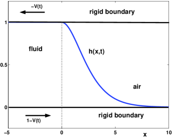
Figure 1: A two-dimensional Couette flow with a free boundary, in the reference frame co-moving with the contact line.

By using asymptotic analysis and the lubrication approximation, Benilov and Vynnycky [1] derived the following nonlinear advection–diffusion equation for the free boundary $h(x,t)$ of the fluid flow:

$$\frac{\partial h}{\partial t}+\frac{\partial}{\partial x}\left[\frac{h^{3}}{3}\left(\alpha^{3}\frac{\partial^{3}h}{\partial x^{3}}+\frac{\partial h}{\partial x}\right)+(1-V(t))h\right]=0,\quad x>0,\;\;t>0,$$ (1)

The boundary conditions $h|_{x=0}=1$ and $h_{x}|_{x=0}=0$ define the normalized thickness and the contact line location, whereas the flux conservation gives the boundary condition for $h_{xxx}|_{x=0}=-\frac{3}{2\alpha^{3}}$. Here and henceforth, we use the subscript to denote the partial derivative. In addition, we fix $\alpha^{3}=3$ for convenience. Existence of weak solutions of the thin-film equation (1) for constant values of $V$ and Neumann boundary conditions on a finite interval was recently shown by Chugunova et al. [4, 5].

Using further asymptotic reductions with

$$h-1=\mathcal{O}(|V|^{-1}),\quad x=\mathcal{O}(|V|^{-1/3}),\quad t=\mathcal{O}(|V|^{-4/3}),\quad\mbox{\rm as}\quad|V|\to\infty,$$ (2)

Benilov and Vynnycky [1] reduced the nonlinear equation (1) with $\alpha^{3}=3$ to the linear advection–diffusion equation:

$$\frac{\partial h}{\partial t}+\frac{\partial^{4}h}{\partial x^{4}}=V(t)\frac{\partial h}{\partial x},\quad x>0,\;\;t>0,$$ (3)

subject to the boundary conditions

$$h|_{x=0}=1,\quad h_{x}|_{x=0}=0,\quad h_{xxx}|_{x=0}=-\frac{1}{2},\quad t\geq 0,$$ (4)

Physically relevant solutions corresponds to the monotonically decreasing solutions with $h\to h_{\infty}$ and $h_{x},h_{xx}\to 0$ as $x\to\infty$, where $h_{\infty}<1$. We note that any constant value of $h_{\infty}$ is allowed thanks to the invariance of the linear advection–diffusion equation (3) with respect to the shift and scaling transformations. Indeed, if $h(x,t)$ solves the boundary–value problem (3)–(4) such that $h\to 0$ as $x\to\infty$, then $\tilde{h}(\tilde{x},\tilde{t})$ given by

$$\tilde{h}(\tilde{x},\tilde{t})=h_{\infty}+(1-h_{\infty})h(x,t),\quad\tilde{x}=(1-h_{\infty})^{1/3}x,\quad\tilde{t}=(1-h_{\infty})^{4/3}t,$$ (5)

for any $h_{\infty}<1$, solves the same advection–diffusion equation (3) with the same boundary conditions (4) but with the variable velocity $\tilde{V}(\tilde{t})=\frac{V(t)}{1-h_{\infty}}$ and with the asymptotic behavior $h\to h_{\infty}$ as $x\to\infty$.

With three boundary conditions at $x=0$ and the decay conditions for $h$ as $x\to\infty$, the initial-value problem for equation (3) is over-determined and the third (over-determining) boundary condition at $x=0$ is used to find the dependence of $V$ on $t$. Local existence of solutions to the boundary–value problem (3)–(4) was proved by Pelinovsky et al. [7] using Laplace transform in $x$ and the fractional power series expansion in powers of $t^{1/4}$.

We shall consider the time evolution of the boundary–value problem (3)–(4) starting with the initial data $h|_{t=0}=h_{0}(x)$ for a suitable function $h_{0}$. For physically relevant solutions, we assume that the profile $h_{0}(x)$ decays monotonically to a constant value as $x\to\infty$ and that $0$ is a non-degenerate maximum of $h_{0}$ such that $h_{0}(0)=1$, $h_{0}^{\prime}(0)=0$, and $h_{0}^{\prime\prime}(0)<0$. The solution $h(x,t)$ may lose monotonicity in $x$ during the dynamical evolution because of the boundary value

$$\beta(t):=h_{xx}(0,t)$$ (6)

crosses zero from the negative side. In this case, we say that the flow becomes non-physical for further times and the model (3)–(4) breaks. Simultaneously, this may mean that the velocity $V(t)$ blows up to infinity, because for sufficiently strong solutions of the advection–diffusion equation (3), the velocity $V(t)$ satisfies the dynamical equation

$$h_{xxxxx}(0,t)=V(t)\beta(t),$$ (7)

which follows by differentiation of (3) in $x$ and setting $x\to 0$.

Based on numerical computations of the thin-film equations (1), Benilov and Vynnycky [1] claim that for any physically relevant initial data $h_{0}$, there is a finite positive time $t_{0}$ such that $V(t)$ tends to negative infinity and $\beta(t)$ approaches zero as $t\nearrow t_{0}$, whereas the profile $h(x,t_{0})$ remains a smooth and decreasing function for $x>0$. Moreover, they claim that $V(t)$ behaves near the blowup time as the logarithmic function of $t$:

$$V(t)\sim C_{1}\log(t_{0}-t)+C_{2},\quad\mbox{\rm as}\quad t\nearrow t_{0},$$ (8)

where $C_{1}$, $C_{2}$ are positive constants. The same properties of the blow up of contact lines were observed in [1] in numerical simulations of the reduced model (3)–(4). We point out that the numerical simulations in [1] are based on COMSOL built-in algorithms.

The goal of this paper is to simulate numerically the behavior of the velocity $V(t)$ near the blow-up time under different physically relevant initial data $h_{0}(x)$. Our technique is based on the reformulation of the boundary-value problem (3)–(4), which will be suitable for an application of the direct finite-difference method. We will approximate the behavior of the velocity $V(t)$ from the dynamical equation (7) rewritten in finite differences. The numerical computations reported in this paper were performed by using the MATLAB software package.

As the main outcome, we confirm that all physically relevant initial data including those with positive initial velocity will result in blow-up of $V(t)$ to negative infinity in a finite time. At the same time, we show that the power function

$$|V(t)|\sim\frac{c}{(t_{0}-t)^{p}},\quad\text{as}\quad t\nearrow t_{0},$$ (9)

with $c>0$ and $p\approx 0.5$ fits our numerical data better than the logarithmic function (8) near the blow-up time $t_{0}$. We explain why the behavior $|V(t)|=\mathcal{O}((t_{0}-t)^{-1/2})$ as $t\nearrow t_{0}$ is highly expected for solutions of the boundary–value problem (3)–(4). We believe that the incorrect logarithmic law (8) is an artefact of the COMSOL built-in algorithms used in [1].

We shall mention two recent relevant works on the same problem. Firstly, existence of self-similar solutions of the linear advection–diffusion equation (3) was proved by Pelinovsky and Giniyatullin [8]. The self-similar solutions are given by

$$V(t)=\frac{t_{0}V_{0}}{(t_{0}-t)^{3/4}},\quad h(x,t)=f(\xi),\quad\xi=\frac{x}{(t_{0}-t)^{1/4}},$$ (10)

with $t_{0}>0$ and $V_{0}>0$, where $f(\xi)$ is a suitable function. Although the self-similar solutions (10) satisfy the decay condition at infinity, and the first two boundary conditions (4), the third boundary condition $h_{xxx}|_{x=0}=-\frac{1}{2}$ is not satisfied and is replaced with $h_{xxx}|_{x=0}=\gamma_{0}V(t)$ for a fixed $\gamma_{0}<0$. Consequently, the self-similar solution (10) predicts blows up in a finite time with positive $V(t)$ and positive $\beta(t)$. Although the scaling of the self-similar solution (10) is compatible with the scaling transformation (2) used in the derivation of the linear advection–diffusion equation (3), it does not satisfy the physical requirements of the Couette flow on Figure 1.

Secondly, Chugunova et al. [3] constructed steady state solutions of the boundary–value problem (3)–(4) and showed numerically that these steady states can serve as attractors of the bounded dynamical evolution of the model. Both the steady states and the initial conditions that lead to bounded dynamics of the model are not physically acceptable as $h_{0}$ has to be monotonically increasing with $h\to h_{\infty}>1$ as $x\to\infty$. Note that both $V$ and $\beta$ are positive for the steady states of the boundary–value problem (3)–(4).

To simulate the boundary–value problem (3)–(4), a different numerical method is proposed in [3]. This method is still based on finite differences and MATLAB software package. Because the fourth-order derivative term is approximated implicitly and the first-order derivative term is approximated explicitly, the system of finite-difference equations was closed in [3] without any additional equation on the velocity $V(t)$. Consequently, $V(t)$ was found from the system of finite-difference equations.

We also mention that both recent works of [8] and [3] used a priori energy estimates and found some sufficient conditions, under which the smooth physically relevant solutions of the boundary–value problem (3)–(4) blows up in a finite time. In particular, if $V(t)>-1$, or $\beta(t)<0$, or $V(t)\beta(t)^{2}<0$, the smooth solution $h(x,t)$ blows up in a finite time. However, these sufficient conditions do not eliminate existence of smooth physically relevant solutions, for which $V(t)$ oscillates and $\beta(t)$ decays to zero as $t\to\infty$.

The remainder of our paper is organized as follows. Section 2 outlines the numerical method for approximations of the boundary–value problem (3)–(4). Section 3 presents the numerical simulations of the boundary–value problem truncated on the finite interval $[0,L]$ for sufficiently large $L$. Section 4 inspects different blow-up rates of the singular behavior of the velocity $V(t)$ near the blow-up time. Section 5 summarizes our findings.

2 Numerical method

In what follows, we set $u:=h_{x}$, and reformulate the boundary-value problem (3)–(4) in the equivalent form. Differentiating equation (3) with respect to $x$, we obtain

$$\frac{\partial u}{\partial t}+\frac{\partial^{4}u}{\partial x^{4}}=V(t)\frac{\partial u}{\partial x},\quad x>0,\quad t>0.$$ (11)

We also rewrite boundary conditions in (4) as follows:

$$u|_{x=0}=0,\quad u_{xx}|_{x=0}=-\frac{1}{2},\quad u_{xxx}|_{x=0}=0,\quad t\geq 0.$$ (12)

Here the third boundary condition $u_{xxx}|_{x=0}=h_{xxxx}|_{x=0}=0$ follows from applying the boundary conditions $h|_{x=0}=1$ and $h_{x}|_{x=0}=0$ to the fourth-order equation (3) as $x\rightarrow 0$. After the reformulation, the dynamical equation (7) can be recovered by taking the limit $x\rightarrow 0$ in (11):

$$u_{xxxx}(0,t)=V(t)u_{x}(0,t),\quad t\geq 0,$$ (13)

provided that the solution $u$ remains smooth at the boundary $x=0$.

A suitable two-parameter initial condition $u|_{t=0}=u_{0}(x)$ for the boundary–value problem (11)–(12) can be chosen in the form

$$u_{0}(x)=-\frac{1}{4}e^{-ax}x[4+(4a+1)x+a(2a+1)x^{2}+bx^{3}],$$ (14)

where parameters $a>0$ and $b\geq 0$ are arbitrary. For simplicity, the constraint

$$\beta(t)=h_{xx}|_{x=0}=u_{x}|_{x=0}<0$$

at the initial time $t=0$ is standardized to $\beta(0)=-1$. Note that $u_{0}(x)$ and its derivatives decay to zero exponentially fast as $x\to\infty$, which still imply that $h_{0}(x)=1+\int_{0}^{x}u_{0}(x^{\prime})dx^{\prime}$ decays to some constant value $h_{\infty}$ as $x\to\infty$. Because $u_{0}(x)<0$ for all $x>0$, $h_{0}$ is a monotonically decreasing function and $h_{\infty}<1$.

Figure 2 shows a particular example of the initial function (14) for $a=0.5$ and $b=0$.

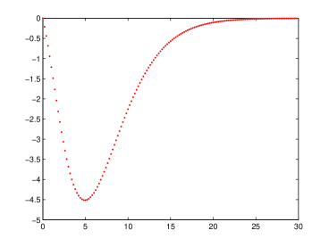
Figure 2: The initial function (14) with $a=0.5$ and $b=0$.

We approximate solutions of the boundary–value problem (11)–(12) with the second-order central-difference method. Consider a set of $N+2$ equally spaced ordered grid points $\{x_{n}\}_{n=0}^{N+1}$ on the interval $[0,L]$, for sufficiently large $L$ so that $u|_{x=L}$ and $u_{xx}|_{x=L}$ are approximately zero. For any fixed $t>0$, let $u_{n}(t)$ denote the numerical approximation of $u(x,t)$ at $x=x_{n}$, and let $\Delta x$ denote the equal step size between adjacent grid points.

By applying the second-order central-difference formulas to partial derivatives in the fourth-order equation (11) at each $x=x_{n}$, we obtain the differential equations:

$$\frac{du_{n}}{dt}=V(t)\frac{u_{n+1}-u_{n-1}}{2(\Delta x)}-\frac{u_{n+2}-4u_{n+1}+6u_{n}-4u_{n-1}+u_{n-2}}{(\Delta x)^{4}},$$ (15)

which are accurate up to the $\mathcal{O}(\Delta x^{2})$ truncation error. Since $u_{0}=u(0,t)=0$ and $u_{N+1}=u(L,t)=0$ for all $t\geq 0$, the above formula needs only to be applied to $N$ interior points $\{x_{n}\}_{n=1}^{N}$ with the necessity to approximate $u_{-1}$ for the grid point $x_{1}$ and $u_{N+2}$ for the grid point $x_{N}$. The value of $u_{-1}$ can be found from the boundary condition:

$$u_{xx}|_{x=0}=-\frac{1}{2}\quad\Rightarrow\quad\frac{u_{-1}-2u_{0}+u_{1}}{(\Delta x)^{2}}=-\frac{1}{2}\quad\Rightarrow\quad u_{-1}=-u_{1}-\frac{1}{2}(\Delta x)^{2},$$

and $u_{N+2}$ can be found from the decay condition:

$$u_{xx}|_{x=L}=0\quad\Rightarrow\quad\frac{u_{N}-2u_{N+1}+u_{N+2}}{(\Delta x)^{2}}=0\quad\Rightarrow\quad u_{N+2}=-u_{N},$$

which are again accurate up to the $\mathcal{O}(\Delta x^{2})$ truncation error. It remains to define $V(t)$ from the third boundary condition $u_{xxx}|_{x=0}=0$.

The velocity $V(t)$ can be expressed by applying the central–difference approximation to the dynamical equation (13):

$$V(t)=\frac{u_{xxxx}|_{x=0}}{u_{x}|_{x=0}}\quad\Rightarrow\quad V(t)=\frac{2(u_{2}-4u_{1}+6u_{0}-4u_{-1}+u_{-2})}{(\Delta x)^{3}(u_{1}-u_{-1})},$$ (16)

where $u_{-2}$ can be found from the third boundary condition in (12):

$$u_{xxx}|_{x=0}=0\quad\Rightarrow\quad\frac{u_{2}-2u_{1}+2u_{-1}-u_{-2}}{(\Delta x)^{3}}=0\quad\Rightarrow\quad u_{-2}=u_{2}-4u_{1}-(\Delta x)^{2}.$$

Writing the system of differential equations (15) in the matrix form

$$\frac{d\boldsymbol{u}}{dt}=\boldsymbol{A}\boldsymbol{u}+\boldsymbol{b},$$

we use Heun’s method to evaluate solutions of the system of differential equations. Let $\boldsymbol{u}_{k}$ denote the numerical approximation of $\boldsymbol{u}(t)$ at $t=t_{k}$ and let $\Delta t$ denote the time step size (not necessarily constant). By Heun’s method, we obtain the iterative rule

$$\boldsymbol{u}_{k+1}=\boldsymbol{u}_{k}+\frac{\Delta t}{2}[(\boldsymbol{A}_{k}\boldsymbol{u}_{k}+\boldsymbol{b})+(\boldsymbol{A}_{k+1}\boldsymbol{u}_{k+1}+\boldsymbol{b})],$$ (17)

where the initial vector $\boldsymbol{u}_{0}$ is obtained from the initial condition (14). Note that the coefficient matrix $\boldsymbol{A}$ depend on $t$ since it is defined by the variable velocity $V(t)$. Nevertheless, ${\bf b}$ is constant in $t$. The global error of Heun’s method is $\mathcal{O}(\Delta t^{2})$, so the global truncation error for the numerical approximation is $\mathcal{O}(\Delta x^{2}+\Delta t^{2})$.

The explicit version of Heun’s method is stable only when

$$\Delta t\leq\displaystyle\frac{1}{8}(\Delta x)^{4}.$$

Therefore, in practice we shall use the implicit Heun’s method (which is stable for all $\Delta t>0$), by solving the system of linear equations

$$(\boldsymbol{I}-\frac{\Delta t}{2}\boldsymbol{A}_{k+1})\boldsymbol{u}_{k+1}=(\boldsymbol{I}+\frac{\Delta t}{2}\boldsymbol{A}_{k})\boldsymbol{u}_{k}+\Delta t\boldsymbol{b},$$ (18)

where $\boldsymbol{I}$ is the identity matrix. However, because the coefficient matrix $\boldsymbol{A}_{k+1}$ on the left-hand side contains an unknown value of $V(t_{k+1})$, a prediction-correction method is necessary for solving this system of equations as follows. First, $\boldsymbol{A}_{k+1}$ is approximated using $\boldsymbol{A}_{k}$ to predict the value of $\boldsymbol{u}_{k+1}^{*}$, which is then used to predict the value of $V(t_{k+1}^{*})$ using equation (16). Second, $\boldsymbol{A}_{k+1}$ is updated from the prediction $V(t_{k+1}^{*})$ to obtain the corrected values of $\boldsymbol{u}_{k+1}$ and $V(t_{k+1})$. Since the implicit method is used in both prediction and correction steps, the unconditional stability is preserved.

3 Blow-up of the velocity $V$ of contact lines

We use the finite-difference method to compute approximation of the boundary–value problem (11)–(12), after truncation on the finite interval $[0,L]$ with sufficiently large $L$. Since the time evolution features blow-up in a finite time, an adaptive method is used to adjust the time step $\Delta t$ after each iteration to maintain the local truncation error of the numerical method at a certain tolerance level.

Figure 3 shows the numerical approximation of the boundary–value problem (11)–(12) for the initial function (14) with $a=0.5$ and $b=0$ (the one shown on Figure 2). The initial velocity is determined from this initial condition by equation (13) as $V(0)=-1.25$. The top left panel of the figure shows the profile of $u(x,t)$ versus $x$ at different values of $t$ until the terminal time $T$ of our computations. The top right panel of the figure shows the change of the velocity $V(t)$ in time $t$ computed dynamically from equation (16). The bottom left panel shows the boundary value $\beta(t)=u_{x}|_{x=0}$ versus $t$ and the bottom right panel shows the boundary value $u_{xxxx}|_{x=0}$ versus $t$.

It is clear from the top panels that the velocity $V$ diverges towards $-\infty$ at $t\approx 1.9$, whereas the solution $u(x,t)$ remains regular near the blow-up time. Recall that the velocity $V(t)$ is determined from equation (13) by the quotient of $u_{xxxx}(0,t)$ and $\beta(t)=u_{x}(0,t)$, where $\beta(t)$ must be strictly negative for all $t>0$ for physically acceptable solutions. We can see from the bottom panels that the value of $\beta$ is about to cross zero from the negative side at the blow-up time, whereas $u_{xxxx}(0,t)$ is also approaching zero but at a much slower rate than $\beta(t)$. This also indicates that $V(t)$ is approaching negative infinity at the blow-up time.

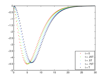
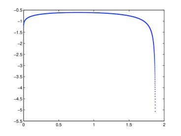
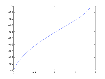
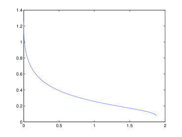
Figure 3: Numerical solution of the boundary-value problem (11)–(12), where $u_{0}$ is given by (14) with $a=0.5$ and $b=0$. Top left: The profile of $u$ versus $x$ at different time $t$. Top right: Velocity of the contact line $V$ versus $t$. Bottom left: The boundary value $\beta=u_{x}|_{x=0}$ versus $t$. Bottom right: The boundary value $u_{xxxx}|_{x=0}$ versus $t$.

To measure the error of numerical computations, we shall derive dynamical constraints on the time evolution of a smooth solution of the boundary–value problem (11)–(12). Differentiating equation (11) with respect to $x$ once and twice and taking the limit $x\rightarrow 0$, we obtain

$$\frac{d\beta}{dt}+\frac{\partial^{5}u}{\partial x^{5}}\biggr{|}_{x=0}=-\frac{1}{2}V(t)$$ (19)

and

$$\frac{\partial^{6}u}{\partial x^{6}}\biggr{|}_{x=0}=0.$$ (20)

Using equation (20), we determine $u_{-3}$ at $x=x_{-3}$ from the central–difference approximation:

$$\frac{u_{3}-6u_{2}+15u_{1}-20u_{0}+15u_{-1}-6u_{-2}+u_{-3}}{(\Delta x)^{6}}=0$$

$$\phantom{texttexttexttexttexttext}\Rightarrow\quad u_{-3}=-u_{3}+12u_{2}-24u_{1}+\frac{3}{2}(\Delta x)^{2}.$$

Then, the value of $d\beta/dt$ is approximated from equations (16) and (19):

$$\beta^{\prime}(t)=-\frac{u_{3}-4u_{2}+5u_{1}-5u_{-1}+4u_{-2}-u_{-3}}{2(\Delta x)^{5}}-\frac{u_{2}-4u_{1}+6u_{0}-4u_{-1}+u_{-2}}{(\Delta x)^{3}(u_{1}-u_{-1})}.$$ (21)

Comparing the value of $\beta^{\prime}(t)$ determined from equation (21) with the central-difference approximation for the numerical derivative

$$\beta^{\prime}(t_{l})=\frac{\beta(t_{k+1})-\beta(t_{k-1})}{t_{k+1}-t_{k-1}},$$ (22)

we can estimate the numerical error of the solution at the boundary $x=0$.

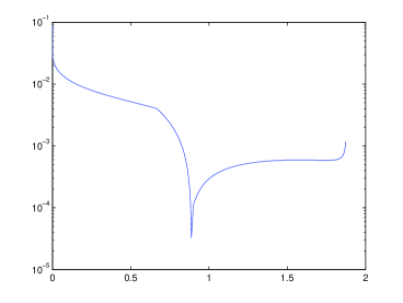
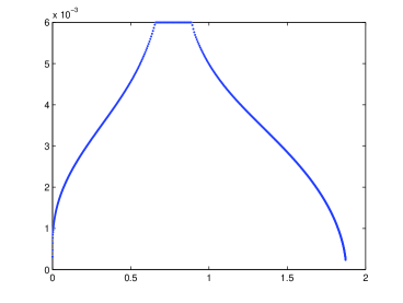
Figure 4: Left: Error of $\beta^{\prime}(t)$ versus $t$. Right: Time step size $\Delta t$ versus $t$.

Figure 4 (left) compares the value of $\beta^{\prime}(t)$ between equations (21) and (22). The error remains small, therefore, the assumption that the solution is smooth (or at least $C^{6}$) at the boundary $x=0$ is valid up to numerical accuracy.

Figure 4 (right) shows the time step size $\Delta t$ adjusted to preserve the same level of the local error of $10^{-5}$. We set $\Delta t=0.006$ if the error estimation procedure yields larger values of $\Delta t$. This truncation is needed because the error drops significantly near $t\approx 0.8$, and the error estimation procedure would otherwise produce large values of $\Delta t$.

We have performed computations with other initial conditions from the two-parameter family of functions in (14). Figure 5 (left) shows the dynamical evolution of the velocity $V$ starting with a positive velocity $V(0)=2.35$, which is determined from the initial function (14) with $a=0.5$ and $b=0.6$. Although the terminal time $T\approx 28$ is much larger compared with the case of the negative initial velocity on Figure 3, a blow-up is still detected from this initial condition. The solution $u(x,t)$ looks similar to the solution shown in Figure 3 (top left) and hence is not shown.

Figure 5 (right) shows the adjusted time step size. We note that the time step size is small at the initial time because the smooth solution appears from the initial condition, which does not satisfy infinitely many constraints of the boundary–value problem (11)–(12). It is also small near the terminal time because of the blow-up of the smooth solution. But $\Delta t$ is not too small at intermediate values of $t$, when the solution is at a slowly varying phase. During this slowly varying phase, $V(t)$ is nearly constant but $\beta(t)$ changes nearly linearly in time (similarly to Figure 3 (bottom left) and hence is not shown).

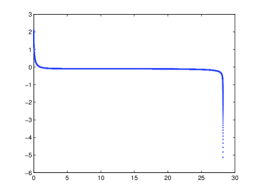
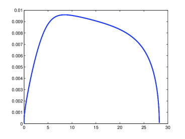
Figure 5: Numerical solution of the boundary-value problem (11)–(12), where $u_{0}$ is given by (14) with $a=0.5$ and $b=0.6$. Left: Velocity of the contact line $V$ versus $t$. Right: Time step size $\Delta t$ versus $t$.

Figure 6 illustrates the dynamical evolution of the velocities $V(t)$ under different initial conditions given by the two-parameter function (14). From these plots, together with the previous examples, it is clear that the blow-up time depends on the initial velocity $V(0)$ and a large positive initial velocity leads to a much longer slowly varying phase before the solution blows up. Nevertheless, the blow-up in a finite time is unavoidable for any physically acceptable initial conditions.

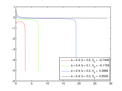
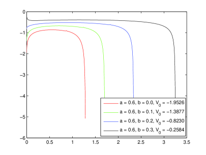
Figure 6: Behavior of the velocity $V$ versus $t$ for different initial conditions given by the two-parameter function (14).

4 Rate of blow-up

In order to determine numerically the blow-up time $t_{0}$ and the rate of blow-up of the velocity $V$, we will fit the numerical data near the terminal time $T$ of our computations with either the logarithmic function (8) or the power function (9).

For the logarithmic function (8), we first differentiate both sides of the expression with respect to $t$ and take the inverse:

$$\frac{dV}{dt}=-\frac{C_{1}}{t_{0}-t}\quad\Rightarrow\quad\biggr{(}\frac{dV}{dt}\biggr{)}^{-1}=\frac{t}{C_{1}}-\frac{t_{0}}{C_{1}}.$$ (23)

Then the constants $C_{1}$ and $t_{0}$ can be determined from a linear regression applied to equation (23). We will skip the numerical procedure for determining the values of $C_{2}$ since it does not affect the blow-up behavior of $V$.

For the power function (9), we can take the logarithm of both sides of the expression

$$\log(-V(t))=\log c-p\log(t_{0}-t)$$

and then differentiate the above expression:

$$\frac{1}{V(t)}\frac{dV}{dt}=\frac{p}{t_{0}-t}\quad\Rightarrow\quad V(t)\biggr{(}\frac{dV}{dt}\biggr{)}^{-1}=\frac{t_{0}}{p}-\frac{t}{p}.$$ (24)

The constants $p$ and $t_{0}$ can now be determined from a linear regression applied to equation (24).

In practice, we found that the blow-up rate $p$ in the power law or the coefficient $C_{1}$ in the logarithmic law vary with different time windows (i.e. the range of $t$ which is used to fit the data). The following output gives a comparison of numerical data under different time windows and different tolerance levels, using the initial condition (14) with $a=0.5$ and $b=0$. Here starting time means the time $t$ at which we start to fit the data, and Error is the mean squared error (MSE) defined by

$$\text{MSE}:=\frac{1}{n-3}\sum(V_{\text{obs}}-V_{\text{fit}})^{2},$$

where $n$ is the total number of data points used in the regression.

Initial condition: a = 0.5, b = 0; initial velocity: V(0) = -1.2500

Tolerance level: 0.0001, number of iterations: 330, terminal time = 1.8729
  Starting time    Blowup time t0    Blowup rate p or C1      Error
powerlaw:
         1.8176         1.8749            0.3916           0.000017
         1.8356         1.8752            0.3994           0.000003
         1.8550         1.8756            0.4104           0.000000
loglaw:
         1.8176         1.8678            0.5371          23.732740
         1.8356         1.8695            0.6135          33.681247
         1.8550         1.8716            0.7578          68.934686

Tolerance level: 1e-006, number of iterations: 1448, terminal time = 1.8732
  Starting time    Blowup time t0    Blowup rate p or C1      Error
powerlaw:
         1.8172         1.8753            0.3927           0.000033
         1.8360         1.8757            0.4009           0.000006
         1.8547         1.8760            0.4118           0.000000
loglaw:
         1.8172         1.8688            0.5500          25.226547
         1.8360         1.8705            0.6343          33.937325
         1.8547         1.8724            0.7854          58.894321

The above table shows that the errors from the logarithmic law (8) are much larger than the errors from the power law (9) in all cases. Also, the error of the power law reduces as the time window moves closer to the blow-up time, whereas the error of the logarithmic law increases. Moreover, the blow-up times $t_{0}$ determined from the logarithmic law are smaller than the terminal time $T$ of our computations. Hence, the logarithmic law deviates from the numerical data near the blow-up time. As we can see in Figure 7, the power function (9) fits our numerical data much better than the logarithmic function (8).

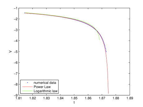
Figure 7: Comparison between data fitting with the logarithmic law (8) and the power law (9).

In order to confirm that the blow-up of the velocity $V$ occurs according to the power law (9) compared to the logarithmic law (8), we use the scaling transformations suggested in [1] and replace the time variable $t$ by the new variable

$$T:=\int_{0}^{t}(1+V^{2n}(t^{\prime}))dt^{\prime},$$ (25)

where $n$ is a positive integer. In new time variable with $V(t)\equiv V(T)$, the model (11) is rewritten in the form

$$\frac{\partial u}{\partial T}=\frac{1}{1+V^{2n}}\left(V\frac{\partial u}{\partial x}-\frac{\partial^{4}u}{\partial x^{4}}\right),\quad x>0,\quad T>0,$$ (26)

whereas the boundary conditions or the numerical method are unaffected. With the power law (9) as $t\nearrow t_{0}$, the new time variable $T$ in (25) approaches a finite limit if $2np<1$ and becomes infinite if $2np\geq 1$. With the logarithmic law (8), the new time variable $T$ would always approach a finite limit for any integer $n$.

Figure 8 shows the dependence of $V$ versus the rescaled time variable $T$ for $n=1$ (left) and $n=2$ (right). It is obvious that the blow up occurs in finite $T$ time if $n=1$ and in infinite $T$ time if $n=2$, which corroborates well with the previous numerical data suggesting that $p<0.5$. This figure rules out the validity of the logarithmic law (8). We have checked that the rescaled time variable $T$ for $n\geq 3$ also extends to infinite times, similarly to the result for $n=2$.

We note that the dependence of $V$ versus the original time variable $t$ can be obtained by numerical integration of the integral in (25). We have checked that both time evolutions of $V$ in $T$ with $n=1$ and $n=2$ recover the same behavior of $V$ in $t$, which resembles the top left panel of Figure 3 except times near the blow-up time, where the computational error becomes more significant.

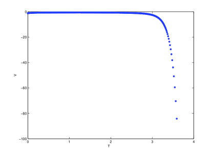
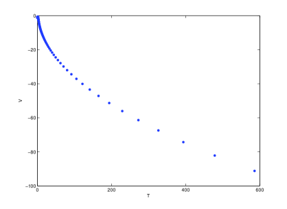
Figure 8: Behavior of the velocity $V$ versus $T$ given by the scaling transformation (25) with $n=1$ (left) and $n=2$ (right).

Using the scaling transformation (25) with $n=2$ in the case when $T\to\infty$ as $t\to\infty$, we can define a more accurate procedure of detecting the blow-up rate $p$ in the power law (9). First, we note that if $|V(t)|=\mathcal{O}((t_{0}-t)^{-p})$ as $t\nearrow t_{0}$, then $T=\mathcal{O}((t_{0}-t)^{1-4p})$ as $t\nearrow t_{0}$. Hence $V(T)=\mathcal{O}(T^{q})$ as $T\to\infty$ with $q:=\frac{p}{4p-1}$. Using now the linear regression in log-log variables for $T$ and $V$, we can estimate the coefficient $q$, and then $p$. The following table shows several computations of $q$ and $p$ for different initial and terminal times $T$. All other parameters are fixed similarly to the previous numerical computations.

Starting time    Terminal time    Regression slope q    Blow-up rate p
     36.0943         723.3424           0.5345              0.4697
    121.7362         723.3424           0.5221              0.4797
    272.5828       78034.1670           0.5044              0.4956
   2393.6301       78034.1670           0.4997              0.5003

The results of data fitting suggest that the power law (9) gives a consistent estimation of the blow-up rate $p$, with $p\approx 0.5$. Let us now discuss why the behavior $|V(t)|=\mathcal{O}((t_{0}-t)^{-1/2})$ as $t\nearrow t_{0}$ appears a generic feature of smooth solutions of the boundary–value problem (11)–(12).

Using equations (13) and (19), we obtain the dynamical equation on $\beta(t)=u_{x}|_{x=0}$:

$$\frac{d\beta}{dt}=-\frac{u_{xxxx}|_{x=0}}{2\beta(t)}-u_{xxxxx}|_{x=0},\quad t\geq 0.$$ (27)

Let us now assume that there is $t_{0}>0$ such that

$$\beta(t)\to 0,\quad u_{xxxx}|_{x=0}\to a_{4},\quad u_{xxxxx}|_{x=0}\to a_{5},\quad\mbox{\rm as}\quad t\nearrow t_{0},$$ (28)

where $a_{4}\neq 0$ and $|a_{5}|<\infty$. Solving the differential equation (27) near the time $t=t_{0}$, we obtain

$$\beta^{2}(t)=a_{4}(t_{0}-t)+\mathcal{O}(t_{0}-t)^{3/2},\quad\Rightarrow\quad V(t)=\sqrt{\frac{a_{4}}{t_{0}-t}}+\mathcal{O}(1),\quad\mbox{\rm as}\quad t\nearrow t_{0},$$ (29)

under the constraint that $a_{4}>0$. The asymptotic rate (29) corresponds to the power law (9) with $p=0.5$.

Figure 9 shows the behavior of absolute values of $u_{x}|_{x=0}$ (left) and $u_{xxxx}|_{x=0}$ (right) versus the rescaled time variable $T$ given by (25) with $n=2$. We can see that the assumption $a_{4}>0$, that is, $u_{xxxx}|_{x=0}$ is bounded away from zero near the blow-up time, is justified numerically. We note that the time evolution in the rescaled time variable $T$ allows us to identify this property better than the time evolution in the original time variable $t$, which is shown on the bottom right panel of Figure 3. We have also checked from the linear regression in log-log coordinates that $|\beta(t)|=\mathcal{O}((t_{0}-t)^{p})$ as $t\nearrow t_{0}$ with $p\approx 0.5$, in consistency with the asymptotic rate (29).

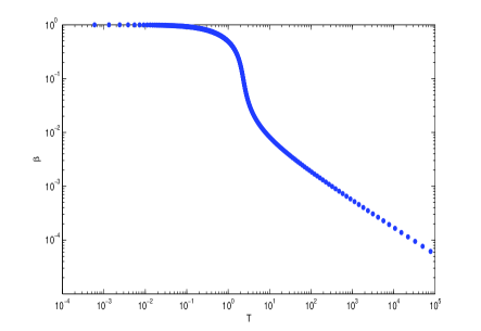
Figure 9: Behavior of $|u_{x}|_{x=0}|$ (left) and $u_{xxxx}|_{x=0}$ (right) versus $T$ given by the scaling transformation (25) with $n=2$. The logarithmic scaling is used for $T$ and $\beta$ variables.

5 Conclusion

We conclude from the numerical simulations of the boundary–value problem (11)–(12) that, for any suitable initial condition in the two-parameter form (14), there always exists a finite positive time $t_{0}$ such that $V(t)\rightarrow-\infty$ as $t\nearrow t_{0}$, although the blow-up time $t_{0}$ varies from different initial velocity $V(0)$. With a large positive initial velocity $V(0)$, the solution tends to have a longer phase of slow motion before it eventually blows up, whereas a negative initial velocity yields a much smaller value of the blow-up time.

The numerical results also suggest that the behavior of $V(t)$ near the blow-up time satisfies the power law (9), with a blow-up rate $p\approx 0.5$. This numerical observation corroborates a simple analytic theory for the blow-up of the velocity of contact lines in the reduced model (3)–(4). Based on earlier numerical evidences in [1], a similar result should also hold for the nonlinear thin-film equation (1).

An open problem for further studies is to develop a more precise and computationally efficient numerical method for solutions of the boundary–value problem (11)–(12). Because the model equation (11) is already a fourth-order differential equation, we shall avoid using any numerical methods that involves higher-order central differences. In addition, because of the unknown variable $V(t)$, it is difficult to use other higher-order implicit methods to solve the system of differential equations after discretization. Thus, the finite difference method has a limited accuracy. Therefore, a different approach is needed, for instance, by using the collocation method involving the discrete Fourier transform.

References

- [1] E.S. Benilov and M. Vynnycky, “Contact lines with a contact angle”, J. Fluid Mech. 718 (2013), 481–506.
- [2] D.J. Benney and W.J. Timson, “The rolling motion of a viscous fluid on and off a rigid surface”, Stud. Appl. Math. 63 (1980), 93–98.
- [3] M. Chugunova, C.Y. Kao, and S. Seepen, “On Benilov–Vynnycky blow-up problem”, preprint (2013).
- [4] M. Chugunova, M. Pugh, and R. Taranets, “Nonnegative solutions for a long-wave unstable thin film equation with convection”, SIAM J. Math. Anal. 42 (2010), 1826-1853.
- [5] M. Chugunova and R. Taranets, “Qualitative analysis of coating flows on a rotating horizontal cylinder”, Int. J. Diff. Eqs. 2012 (2012), Article ID 570283, 30 pages.
- [6] C.G. Ngan and V.E.B. Dussan, “The moving contact line with a advancing contact angle”, Phys. Fluids 24 (1984), 2785–2787.
- [7] D.E. Pelinovsky, A.R. Giniyatullin, and Y.A. Panfilova, “On solutions of a reduced model for the dynamical evolution of contact lines”, Transactions of Nizhni Novgorod State Technical University n.a. Alexeev N.4 (94) (2012), 45–60.
- [8] D.E. Pelinovsky and A.R. Giniyatullin, “Finite-time singularities in the dynamical evolution of contact lines”, Bulletin of the Moscow State Regional University (Physics and Mathematics) 2012 N.3 (2012), 14–24.