Alternative separation of exchange and correlation energies in multi-configuration range-separated density-functional theory

Abstract

The alternative separation of exchange and correlation energies proposed by Toulouse et al. [Theor. Chem.  Acc. 114, 305 (2005)] is explored in the context of multi-configuration range-separated density-functional theory. The new decomposition of the short-range exchange–correlation energy relies on the auxiliary long-range interacting wavefunction rather than the Kohn–Sham (KS) determinant. The advantage, relative to the traditional KS decomposition, is that the wavefunction part of the energy is now computed with the regular (fully-interacting) Hamiltonian. One potential drawback is that, because of double counting, the wavefunction used to compute the energy cannot be obtained by minimizing the energy expression with respect to the wavefunction parameters. The problem is overcome by using short-range optimized effective potentials (OEPs). The resulting combination of OEP techniques with wavefunction theory has been investigated in this work, at the Hartree-Fock (HF) and multi-configuration self-consistent-field (MCSCF) levels. In the HF case, an analytical expression for the energy gradient has been derived and implemented. Calculations have been performed within the short-range local density approximation on H₂, N₂, Li₂ and H₂O. Significant improvements in binding energies are obtained with the new decomposition of the short-range energy. The importance of optimizing the short-range OEP at the MCSCF level when static correlation becomes significant has also been demonstrated for H₂, using a finite-difference gradient. The implementation of the analytical gradient for MCSCF wavefunctions is currently in

I Introduction

The simultaneous description of dynamical and non-dynamical (static or strong) electron correlation in atomic and molecular systems, using low-cost methodologies, remains a challenge for electronic-structure theory. In particular, standard Kohn–Sham density-functional theory Kohn and Sham (1965) (KS-DFT) approximations have enjoyed success in treating phenomena where the description of short-range dynamical correlation is paramount but they have been unable to provide reliable results whenever static correlation is important—including the description of bond breaking, transition-metal compounds, conjugated polymers, and magnetic materials.

Over the years, a great deal of effort has been devoted to understand the shortcomings of density-functional approximations (DFAs) for the treatment of static correlation and to develop new approximations to address this situation. Within the framework of KS-DFT, the pragmatic unrestricted approach can of course be used for describing bond breaking for example but, in this case, space and spin symmetries are broken which is fundamentally not satisfactory. Recent progress towards DFAs capable of treating static correlation has been made, for example, by Malet and Gori-Giorgi Malet and Gori-Giorgi (2012) and by Becke Becke (2013). Other authors have focussed on ensemble-DFT (E-DFT). The utility of E-DFT has been analyzed by Schipper et al. Schipper et al. (1998) and recent implementations of E-DFT variants have been made by Filatov et al. Filatov and Shaik (1999), by Chai Chai (2012), and by Nygaard and Olsen Nygaard and Olsen (2013).

Beyond the framework of standard KS-DFT, a number of groups have pursued the idea of hybridizing density-functional and multi-configuration self-consistent-field (MCSCF) approaches. The goal of these approaches is to treat static correlation using the flexibility of the MCSCF expansion, whilst treating dynamical correlation using density functionals Colle and Salvetti (1990); Savin (1988, 1989); Miehlich et al. (1997); Gräffenstein and Cremer (2000); Stoll (2003); Ying et al. (2012); Malcolm and McDouall (1998); McDouall (2003); Gräffenstein and Cremer (2005); Gusarov et al. (2004); Nakata et al. (2006); Yamanaka et al. (2006); Ukai et al. (2007); Pérez-Jiménez and Pérez-Jordá (2007). A number of MCSCF-DFT hybrid approaches have been proposed, including the complete-active-space-DFT (CAS-DFT) schemes of Gräffenstein et al. Gräffenstein and Cremer (2000), Gusarov et al. Gusarov et al. (2004), and Miehlich et al. Miehlich et al. (1997) A multi-configuration extension of KS-DFT using optimized effective potential techniques has also been proposed by Weimer et al. Weimer et al. (2008) A challenge for these methodologies is to avoid double counting of correlation effects, as the density functionals utilized in these approaches depend on the MCSCF expansions. Tackling the double counting problem is a difficult task as illustrated by Kurzweil et al. Kurzweil et al. (2009) in their analysis on the mapping of interacting onto partially interacting system.

A key step in avoiding the doubling counting problems of the MCSCF-DFT hybrid approaches was the proposal of Savin et al. Savin (1996); Stoll and Savin (1985) to divide the Coulomb interaction into long-range (lr) and short-range (sr) contributions. The introduction of this range-separated approach has led to a wide variety of hybrid wave-function/DFT approaches; in the present context, we note the multi-configuration short-range DFT (MC-srDFT) approach of Refs. Pedersen, 2004; Fromager et al., 2007, 2009. Range separation has proven to be of great utility for the treatment of dispersion interactions, where the simple physical intuition that interactions are long-ranged can be leveraged to provide a clean division of labour between the density-functional and wave-function contributions.Ángyán et al. (2005); Goll et al. (2005); Toulouse et al. (2009); Fromager et al. (2010); Janesko et al. (2009); Toulouse et al. (2011); Strømsheim et al. (2011) However, for the description of static correlation, this approach is less effective since static correlation may not be interpreted as predominantly long-ranged. Thus, even for systems such as stretched H₂, where static correlation is expected to be dominant, the corresponding short-ranged density-functional still plays a significant role Teale et al. (2010) and errors associated with these approximations can lead to significant errors in binding energies, albeit with an improved shape for the potential energy curve.Fromager et al. (2007) These considerations are reflected in the fact that a recently proposed MC-DFT approach based on a simple linear (rather than range-dependent) decomposition of the Coulomb interaction delivers similar accuracy in practice.Sharkas et al. (2012)

To overcome some of the difficulties associated with the MC-srDFT models for the description of static correlation, Toulouse et al. Toulouse et al. (2005a) proposed an alternative separation of the short-range exchange and correlation energies, which may be more natural in the context of hybrid methodologies that incorporate multi-configurational components. The practical performance of methods using this partitioning is investigated in the present work.

The paper is organized as follows. In Sec. II, exact and approximate formulations of range-separated DFT are presented. The differences between the traditional and the alternative short-range exchange–correlation energy decompositions are highlighted. For the latter, long-range HF and MCSCF approximations are combined with short-range OEPs in order to overcome double counting problems. Details of the various range-separated schemes that have been implemented are given in Sec. III, while the results obtained for H₂, N₂, H₂O, and Li₂ are discussed in Sec. IV. Finally, conclusions are given in Sec. V.

II Theory

In this section, we present the theory underlying the various multi-configuration range-separated DFT models assessed in Sec. IV. We first introduce in Sec. II.1 the exact multi-determinantal extension of KS-DFT based on range separation. The conventional KS decomposition of the short-range exchange–correlation density functional, as well as an alternative one that relies on the long-range interacting wavefunction (rather than the KS determinant), are next discussed in Secs. II.2 and II.3. The combination of OEPs with multi-determinant wavefunctions and density-functionals is then considered in Sec. II.4.1. Models based on HF and MC wavefunctions are discussed in Sec. II.4.2. The derivation of the analytical energy gradient for the OEP optimization at the HF level is finally presented in Sec. II.5. A summary is given in Sec. II.6.

II.1 Multi-determinant range-separated DFT

In multi-determinant range-separated DFT,Savin (1996, 1995); Stoll and Savin (1985) referred to as short-range DFT (srDFT) in the following, the regular two-electron Coulomb interaction is split into long- and short-range parts,

$$w_{\rm ee}(r_{12}) =1/r_{12}=w^{\rm lr,\mu}_{\rm ee}(r_{12})+w^{\rm sr,\mu}_{\rm ee}(r_{12}),$$ (1)

where $\mu$ is a parameter that controls the range separation. In this work, the long-range interaction is based on the error function

$${w^{\rm lr,\mu}_{\rm ee}(r_{12})=\frac{{\rm erf}(\mu r_{12})}{r_{12}}.}$$ (2)

The universal Levy–Lieb functional Levy (1979); Lieb (1983)

$$F[n] =\underset{\Psi\rightarrow n}{\rm min}\langle\Psi|\hat{T}+\hat{W}_{\rm ee}|\Psi\rangle,$$ (3)

where $\hat{T}$ is the kinetic energy operator and $\hat{W}_{\rm ee}$ the two-electron repulsion operator, can then be rewritten as

$$F[n] =F^{\rm lr,\mu}[n]+E^{\rm sr,\mu}_{\rm Hxc}[n],$$ (4)

with the universal long-range functional defined as

$$F^{\rm lr,\mu}[n] =\underset{\Psi\rightarrow n}{\rm min}\langle\Psi|\hat{T}+\hat{W}^{\rm lr,\mu}_{\rm ee}|\Psi\rangle$$

$$=\langle\Psi^{\mu}[n]|\hat{T}+\hat{W}^{\rm lr,\mu}_{\rm ee}|\Psi^{\mu}[n]\rangle.$$ (5)

The minimizing wavefunction $\Psi^{\mu}[n]$ in Eq. (II.1) corresponds to the ground state of the auxiliary long-range interacting system with density $n$. When connecting the auxiliary and physical systems by a generalized adiabatic-connection path,Yang (1998); Teale et al. (2010); Savin et al. (2003) the complementary short-range Hartree–exchange–correlation (srHxc) energy can be expressed as

$$E^{\rm sr,\mu}_{\rm Hxc}[n] =\int^{1}_{\mu/(1+\mu)}\mathcal{W}^{\nu}_{\rm Hxc}[n]\;\mathrm{d}\nu,$$ (6)

where the srHxc integrand is given by

$$\mathcal{W}^{\nu}_{\rm Hxc}[n] =\left\langle\frac{\partial\hat{W}^{\rm lr,\nu/(1-\nu)}_{\rm ee}}{\partial\nu}\right\rangle_{\Psi^{\nu/(1-\nu)}[n]}.$$ (7)

Note that the expression in Eq. (6) relies on the density constraint

$$n_{\Psi^{\nu/(1-\nu)}[n]}({\bf r}) =n({\bf r}),\hskip 14.22636pt0\leq\nu\leq 1.$$ (8)

According to the variational principle Hohenberg and Kohn (1964) and Eq. (4), the exact expression for the ground-state energy of an electronic system becomes

$$E =\underset{n}{\rm min}\left\{F[n]+\int{\rm d}{\bf r}\,v_{\rm ne}({\bf r})\,n({\bf r})\right\}$$

$$=\underset{n}{\rm min}\left\{\langle\Psi^{\mu}[n]|\hat{T}+\hat{W}^{\rm lr,\mu}_{\rm ee}+\hat{V}_{\rm ne}|\Psi^{\mu}[n]\rangle+E^{\rm sr,\mu}_{\rm Hxc}[n]\right\},$$ (9)

where $\hat{V}_{\rm ne}=\int{\rm d}{\bf r}\,v_{\rm ne}({\bf r})\,\hat{n}({\bf r})$ is the nuclear potential operator. The exact ground-state energy can also be obtained by a minimization over wavefunctions

$$E =\underset{\Psi}{\rm min}\left\{\langle\Psi|\hat{T}+\hat{W}^{\rm lr,\mu}_{\rm ee}+\hat{V}_{\rm ne}|\Psi\rangle+E^{\rm sr,\mu}_{\rm Hxc}[n_{\Psi}]\right\}$$

$$=\langle\Psi^{\mu}|\hat{T}+\hat{W}^{\rm lr,\mu}_{\rm ee}+\hat{V}_{\rm ne}|\Psi^{\mu}\rangle+E^{\rm sr,\mu}_{\rm Hxc}[n_{\Psi^{\mu}}],$$ (10)

where the minimizing wavefunction $\Psi^{\mu}$ fulfills the self-consistent equation

$$(\hat{T}+\hat{W}^{\rm lr,\mu}_{\rm ee}+\hat{V}^{\mu}[n_{\Psi^{\mu}}])|\Psi^{\mu}\rangle=\mathcal{E}^{\mu}|\Psi^{\mu}\rangle,$$ (11)

with

$$\hat{V}^{\mu}[n]=\int{\rm d}{\bf r}\,\left(v_{\rm ne}({\bf r})+\frac{\delta E^{\rm sr,\mu}_{\rm Hxc}}{\delta n({\bf r})}[n]\right)\hat{n}({\bf r}).$$ (12)

While $\hat{W}^{\rm lr,\mu}_{\rm ee}$ vanishes and Eq. (11) reduces to the conventional KS equation at $\mu=0$, the full Schrödinger equation is recovered in the $\mu\rightarrow+\infty$ limit, as $\hat{W}^{\rm lr,\mu}_{\rm ee}$ reduces to the regular two-electron repulsion and the short-range interaction vanishes. For intermediate $\mu$ values, $0<\mu<+\infty$, a hybrid wave-function/DFT description is obtained. Then, in contrast to traditional KS-DFT, the exact auxiliary wavefunction $\Psi^{\mu}$ is generally multi-determinantal owing to the explicit description of long-range interactions.

The srDFT approximation obtained by restricting the minimization in Eq. (II.1) to single determinants is in the following referred to as HF-srDFT; this approximation was referred to as range-separated hybrid (RSH) theory in Ref. Ángyán et al., 2005. To describe multi-configurational electronic systems, a long-range MCSCF description has also been proposed,Pedersen (2004); Fromager et al. (2007) leading to the MC-srDFT model. In this work, we consider both schemes.

II.2 KS decomposition of the short-range energy

The conventional decomposition of the srHxc energy is analogous to that in standard KS-DFT Toulouse et al. (2004a),

$$E^{\rm sr,\mu}_{\rm Hxc}[n] =E^{\rm sr,\mu}_{\rm H}[n]+E^{\rm sr,\mu}_{\rm x}[n]+E^{\rm sr,\mu}_{\rm c}[n],$$ (13)

where the short-range Hartree energy is defined as

$$E^{\rm sr,\mu}_{\rm H}[n]=\frac{1}{2}\int\int{\rm d}{\mathbf{r}}{\rm d}{\mathbf{r^{\prime}}}n(\mathbf{r})n(\mathbf{r^{\prime}})w^{\rm sr,\mu}_{\rm ee}\left(|{\bf r}-{\bf r^{\prime}}|\right),$$ (14)

and the exact short-range exchange energy is calculated from the non-interacting KS determinant $\Phi^{\rm KS}[n]$ with density $n$. The Hartree–exchange integrand is then obtained from Eq. (7) by replacing the long-range interacting wavefunction by $\Phi^{\rm KS}[n]$

$$\mathcal{W}^{\nu}_{\rm Hx}[n] =\left\langle\frac{\partial\hat{W}^{\rm lr,\nu/(1-\nu)}_{\rm ee}}{\partial\nu}\right\rangle_{\Phi^{\rm KS}[n]},$$ (15)

which defines the short-range exchange energy, according to Eq. (6), as

$$E^{\rm sr,\mu}_{\rm x}[n] =\int^{1}_{\mu/(1+\mu)}\mathcal{W}^{\nu}_{\rm Hx}[n]\;\mathrm{d}\nu-E^{\rm sr,\mu}_{\rm H}[n]$$ (16)

$$=\langle\Phi^{\rm KS}[n]|\hat{W}^{\rm sr,\mu}_{\rm ee}|\Phi^{\rm KS}[n]\rangle-E^{\rm sr,\mu}_{\rm H}[n].$$

The corresponding correlation integrand is then given by

$$\mathcal{W}^{\nu}_{\rm c}[n] =\mathcal{W}^{\nu}_{\rm Hxc}[n]-\mathcal{W}^{\nu}_{\rm Hx}[n]$$

$$=\left\langle\frac{\partial\hat{W}^{\rm lr,\nu/(1-\nu)}_{\rm ee}}{\partial\nu}\right\rangle_{\Psi^{\nu/(1-\nu)}[n]}-\left\langle\frac{\partial\hat{W}^{\rm lr,\nu/(1-\nu)}_{\rm ee}}{\partial\nu}\right\rangle_{\Phi^{\rm KS}[n]},$$ (17)

leading to the following expression for the exact complementary short-range correlation energy

$$E^{\rm sr,\mu}_{\rm c}[n] =\int^{1}_{\mu/(1+\mu)}\mathcal{W}^{\nu}_{\rm c}[n]\;\mathrm{d}\nu.$$ (18)

Note that, according to Eqs. (4), (II.1) and (16), this energy can also be expressed as

$$E^{\rm sr,\mu}_{\rm c}[n]=E_{\rm c}[n] +\langle\Phi^{\rm KS}[n]|\hat{T}+\hat{W}^{\rm lr,\mu}_{\rm ee}|\Phi^{\rm KS}[n]\rangle$$

$$-\langle\Psi^{\mu}[n]|\hat{T}+\hat{W}^{\rm lr,\mu}_{\rm ee}|\Psi^{\mu}[n]\rangle,$$ (19)

where $E_{\rm c}[n]$ is the regular correlation density-functional energy, recovered in the $\mu=0$ limit. It is clear from Eq. (II.2) that the complementary short-range correlation density functional contains the purely short-range correlation effects as well as their coupling with long-range correlation.Toulouse and Savin (2006) Various short-range functionals have been developed for practical srDFT calculations at the local density (srLDA), Toulouse and Savin (2006); Toulouse et al. (2004b); Paziani et al. (2006) generalized gradient,Heyd et al. (2003); Heyd and Scuseria (2004); Goll et al. (2005); Toulouse et al. (2004a); Goll et al. (2006); Toulouse et al. (2005b) and meta-generalized gradientGoll et al. (2009) levels of approximation. These functionals have been successfully employed with a number of post-HF-srDFT and post-MC-srDFT long-range correlation treatments to describe dispersion. Ángyán et al. (2005); Goll et al. (2005); Toulouse et al. (2009); Fromager et al. (2010); Janesko et al. (2009); Toulouse et al. (2011) However, for systems with significant static correlation, they are usually not accurate enough.Fromager et al. (2007, 2009) To improve upon the description of the short-range energy, we consider in the following an alternative separation of exchange and correlation energies.

II.3 Alternative decomposition of the short-range energy

As pointed out by Toulouse, Gori-Giorgi, and Savin,Toulouse et al. (2005a); Gori-Giorgi and Savin (2009) it is more natural, in the context of srDFT, to define the short-range exchange energy in terms of the multi-determinantal wavefunction $\Psi^{\mu}[n]$ introduced in Eq. (II.1). This observation leads to the following decomposition of the srHxc density-functional energy

$$E^{\rm sr,\mu}_{\rm Hxc}[n]=E^{\rm sr,\mu}_{\rm H}[n]+E^{\rm sr,\mu}_{\rm x,md}[n]+E^{\rm sr,\mu}_{\rm c,md}[n],$$ (20)

where, what is referred to as the short-range multideterminantal (MD) exchange functional in Ref. Gori-Giorgi and Savin, 2009, is defined as

$$E^{\rm sr,\mu}_{\rm x,md}[n]=\langle\Psi^{\mu}[n]|\hat{W}^{\rm sr,\mu}_{\rm ee}|\Psi^{\mu}[n]\rangle-E^{\rm sr,\mu}_{\rm H}[n].$$ (21)

This expression arises naturally from Eqs. (6) and (7) when replacing the $\nu$-dependent wavefunction in the integrand by the one obtained with the lower integration limit $\nu=\mu/(1+\mu)$, namely $\Psi^{\mu}[n]$. We thus define the MD Hartree–exchange integrand as

$$\mathcal{W}^{\mu,\nu}_{\rm Hx,md}[n] =\left\langle\frac{\partial\hat{W}^{\rm lr,\nu/(1-\nu)}_{\rm ee}}{\partial\nu}\right\rangle_{\Psi^{\mu}[n]}.$$ (22)

The short-range MD exchange energy is then obtained as follows, according to Eq. (6),

$$E^{\rm sr,\mu}_{\rm x,md}[n] =\int^{1}_{\mu/(1+\mu)}\mathcal{W}^{\mu,\nu}_{\rm Hx,md}[n]\;\mathrm{d}\nu-E^{\rm sr,\mu}_{\rm H}[n],$$ (23)

leading to Eq. (21). We emphasize that, for $\mu>0$, $\Psi^{\mu}[n]$ differs from the KS determinant. As a result, the expression for the “exchange” energy in Eq. (21) contains a correlation contribution, in addition to the short-range exchange energy. Note also that the complementary short-range correlation functional in Eq. (20) differs from the conventional one introduced in Eq. (13):

$$E^{\rm sr,\mu}_{\rm c,md}[n] =E^{\rm sr,\mu}_{\rm c}[n]+\langle\Phi^{\rm KS}[n]|\hat{W}^{\rm sr,\mu}_{\rm ee}|\Phi^{\rm KS}[n]\rangle$$

$$-\langle\Psi^{\mu}[n]|\hat{W}^{\rm sr,\mu}_{\rm ee}|\Psi^{\mu}[n]\rangle.$$ (24)

This also becomes clear when expressing the MD short-range correlation energy,

$$E^{\rm sr,\mu}_{\rm c,md}[n] =\int^{1}_{\mu/(1+\mu)}\mathcal{W}^{\mu,\nu}_{\rm c,md}[n]\;\mathrm{d}\nu,$$ (25)

in terms of the corresponding correlation integrand

$$\mathcal{W}^{\mu,\nu}_{\rm c,md}[n] =\mathcal{W}^{\nu}_{\rm Hxc}[n]-\mathcal{W}^{\mu,\nu}_{\rm Hx,md}[n]$$

$$=\left\langle\frac{\partial\hat{W}^{\rm lr,\nu/(1-\nu)}_{\rm ee}}{\partial\nu}\right\rangle_{\Psi^{\nu/(1-\nu)}[n]}-\left\langle\frac{\partial\hat{W}^{\rm lr,\nu/(1-\nu)}_{\rm ee}}{\partial\nu}\right\rangle_{\Psi^{\mu}[n]},$$ (26)

which differs from the conventional integrand in Eq. (II.2) only in the use of $\Psi^{\mu}[n]$ rather than $\Phi^{\text{KS}}[n]$ in the last (subtracted) term. Note that the correlation energies $E_{\text{c}}[n]$ and $E^{\rm sr,\mu}_{\rm c,md}[n]$ are related in a simple manner, as seen by inserting Eq. (II.2) into Eq. (II.3) and rearranging,

$$\langle\Psi^{\mu}[n]|\hat{T}+\hat{W}_{\rm ee}|\Psi^{\mu}[n]\rangle+E^{\rm sr,\mu}_{\rm c,md}[n]=\langle\Phi^{\rm KS}[n]|\hat{T}+\hat{W}_{\rm ee}|\Phi^{\rm KS}[n]\rangle+E_{\rm c}[n],$$ (27)

where the long-range correlation and its coupling with the short-range interaction is contained in the expectation value on the left-hand side but in the correlation functional on the right-hand side. Substitution of the srHxc energy decomposition in Eqs. (20) and (21) back into the ground-state energy expression in Eq. (II.1) leads to

$$E=\underset{n}{\rm min}\left\{\langle\Psi^{\mu}[n]|\hat{T}+\hat{W}_{\rm ee}+\hat{V}_{\rm ne}|\Psi^{\mu}[n]\rangle+E^{\rm sr,\mu}_{\rm c,md}[n]\right\}.$$ (28)

Since $\Psi^{\mu}[n_{\Psi^{\mu}}]$=$\Psi^{\mu}$, we conclude from Eq. (II.1) that the exact ground-state energy can be re-expressed as

$$E =\langle\Psi^{\mu}|\hat{T}+\hat{W}_{\rm ee}+\hat{V}_{\rm ne}|\Psi^{\mu}\rangle+E^{\rm sr,\mu}_{\rm c,md}[n_{\Psi^{\mu}}].$$ (29)

We emphasize that the expression in Eq. (29) is exact when the energy is calculated from the self-consistent wavefunction in Eq. (II.1). We here introduce an approximation, the range-separated hybrid model with full-range integrals (RSHf), where the energy in Eq. (29) is instead computed from the HF-srDFT wavefunction. A multi-configuration extension is obtained when using the MC-srDFT rather than HF-srDFT wavefunction, defining thus a range-separated multi-configuration hybrid model with full-range integrals (RSMCHf).

In the RSHf and RSMCHf schemes, the wavefunctions are optimized with the conventional short-range exchange–correlation density-functional, while the energy is computed with the alternative separation of exchange and correlation energies. As discussed in Sec. IV, this approach may not be sufficiently accurate when approximate functionals are used, especially when static correlation becomes important. The alternative decomposition of the short-range energy should then be used for the optimization of the wavefunction. However, unlike in srDFT, the minimization over densities in Eq. (28) cannot be replaced by a minimization over wavefunctions,

$$E\neq\underset{\Psi}{\rm min}\left\{\langle\Psi|\hat{T}+\hat{W}_{\rm ee}+\hat{V}_{\rm ne}|\Psi\rangle+E^{\rm sr,\mu}_{\rm c,md}[n_{\Psi}]\right\},$$ (30)

simply because the minimizing wavefunction would be the ground state of a fully-interacting system, leading thus to double counting. On the other hand, invoking the one-to-one correspondence between densities and local potentials, a multi-determinant extension of KS-OEP schemes can be formulated.

II.4 Multi-determinant range-separated OEP approach

II.4.1 Exact formulation

When using the local potential rather than the density as a basic variable, the exact ground-state energy expression in Eq. (28) can be rewritten as Toulouse et al. (2005a)

$$E= \underset{v}{\rm min}\left\{\langle\Psi^{\mu}[v]|\hat{T}+\hat{W}_{\rm ee}+\hat{V}_{\rm ne}|\Psi^{\mu}[v]\rangle\right.+\left.E^{\rm sr,\mu}_{\rm c,md}[n_{\Psi^{\mu}[v]}]\right\},$$ (31)

where $\Psi^{\mu}[v]$ is the ground state of the long-range interacting Hamiltonian with the local potential $v$:

$$\Psi^{\mu}[v]=\!\operatorname*{arg\,min}\limits_{\Psi}\!\left\{\!\langle\Psi|\hat{T}+\hat{W}^{\rm lr,\mu}_{\rm ee}|\Psi\rangle+\!\!\int\!\!{\rm d}{\mathbf{r}}\,v({\mathbf{r}}){n}_{\Psi}({\bf r})\!\right\}.$$ (32)

Since $\Psi^{\mu}[v]$ is the solution to a (linear) eigenvalue equation, the formulation in Eqs. (31) and (32) will be referred to as non-self-consistent. According to Eq. (25), the MD short-range correlation energy vanishes as $\mu\rightarrow+\infty$ and the minimizing potential in Eq. (31) is simply the nuclear potential. Regular wave-function theory is then recovered. On the other hand, when $\mu=0$, the energy in Eq. (31) reduces to a KS-OEP energy where the exact-exchange (EXX) term Yang and Wu (2002) is used in conjunction with the standard correlation density functional.

When $0<\mu<+\infty$, we obtain a rigorous combination of wave-function and KS-OEP density-functional approaches, referred to as srOEP in the following. According to Eqs. (11), (12) and (29), the exact minimizing potential is then given by

$$v^{\mu}({\bf r})=v_{\rm ne}({\bf r})+\frac{\delta E^{\rm sr,\mu}_{\rm Hxc}}{\delta n({\bf r})}[n_{\Psi^{\mu}}],$$ (33)

which can be rewritten as

$$v^{\mu}({\bf r})=v_{\rm ne}({\bf r}) +\frac{\delta E^{\rm sr,\mu}_{\rm H}}{\delta n({\bf r})}[n_{\Psi^{\mu}}]+\frac{\delta E^{\rm sr,\mu}_{\rm x,md}}{\delta n({\bf r})}[n_{\Psi^{\mu}}]$$

$$+\frac{\delta E^{\rm sr,\mu}_{\rm c,md}}{\delta n({\bf r})}[n_{\Psi^{\mu}}],$$ (34)

in terms of the srHxc decomposition in Eq. (20). Since the MD short-range correlation energy is here an explicit functional of the density, for which local density approximations have been proposed,Toulouse et al. (2005a); Gori-Giorgi and Savin (2009) only the MD short-range exchange part needs to be optimized in Eq. (II.4.1), being an implicit functional of the density according to Eq. (21). Note that the srOEP energy in Eq. (31) can be rewritten as

$$E =\underset{v}{\rm min}\left\{\langle\tilde{\Psi}^{\mu}[v]|\hat{T}+\hat{W}_{\rm ee}+\hat{V}_{\rm ne}|\tilde{\Psi}^{\mu}[v]\rangle+E^{\rm sr,\mu}_{\rm c,md}[n_{\tilde{\Psi}^{\mu}[v]}]\right\},$$ (35)

where the auxiliary wavefunction $\tilde{\Psi}^{\mu}[v]$ is obtained for a given local potential $v$ as follows:

$$\tilde{\Psi}^{\mu}[v]=\operatorname*{arg\,min}\limits_{\Psi} \left\{\langle\Psi|\hat{T}+\hat{W}^{\rm lr,\mu}_{\rm ee}+\hat{V}_{\rm ne}|\Psi\rangle+E^{\rm sr,\mu}_{\rm H}[n_{\Psi}]+E^{\rm sr,\mu}_{\rm c,md}[n_{\Psi}]+\int{\rm d}{\mathbf{r}}\;v({\mathbf{r}})\,{n}_{\Psi}({\bf r})\right\}.$$ (36)

Indeed, as $\tilde{\Psi}^{\mu}[v]$ satisfies the self-consistent equation

$$\left(\hat{T}+\hat{W}^{\rm lr,\mu}_{\rm ee}+\hat{V}_{\rm ne}+\int{\rm d}{\bf r}\,\frac{\delta E^{\rm sr,\mu}_{\rm H}}{\delta n({\bf r})}[n_{\tilde{\Psi}^{\mu}[v]}]\,\hat{n}(\mathbf{r})\right.$$

$$\left.+\int{\rm d}{\bf r}\,\left[\frac{\delta E^{\rm sr,\mu}_{\rm c,md}}{\delta n({\bf r})}[n_{\tilde{\Psi}^{\mu}[v]}]+v({\mathbf{r}})\right]\,\hat{n}(\mathbf{r})\right)|\tilde{\Psi}^{\mu}[v]\rangle$$

$$=\tilde{\mathcal{E}}^{\mu}[v]|\tilde{\Psi}^{\mu}[v]\rangle,$$ (37)

it is clear from Eq. (II.4.1) that the minimum in Eq. (35) is reached for the local potential

$$\tilde{v}^{\mu}({\mathbf{r}})=\frac{\delta E^{\rm sr,\mu}_{\rm x,md}}{\delta n({\mathbf{r}})}[n_{\Psi^{\mu}}]$$ (38)

since $\tilde{\Psi}^{\mu}[\tilde{v}^{\mu}]=\Psi^{\mu}$. The formulation in Eqs. (35) and (36) will be referred to as self-consistent. It is equivalent to the non-self-consistent formulation in Eq. (31) as long as there are no restrictions in the form of the optimized potential. This statement holds if an approximate MD short-range correlation density functional is used in conjunction with approximate long-range interacting HF or MCSCF wavefunctions, as considered in the rest of this work.
Since optimized potentials are usually expanded in a finite basis,Yang and Wu (2002) the non-self-consistent and self-consistent formulations in Eqs. (31) and (35), respectively, may give different results if the basis set in the first formulation is not sufficiently large to describe both short-range Hartree and MD correlation density-functional potentials accurately. The advantage of the second formulation lies in the fact that the basis set is used only to represent the MD exchange part of the short-range potential, see Eq. (38); the remaining Hartree and MD correlation short-range contributions are calculated as functional derivatives, see Eq. (II.4.1). The drawback with respect to the implementation is related to the computation of the energy gradient needed for optimizing the potential. As discussed in Sec. II.5, the gradient requires the calculation of the linear response function for the long-range interacting wavefunction. The self-consistent formulation is thus less trivial to implement, requiring the implementation of second-order functional derivative contributions (kernel) to the linear response equations.Fromager et al. (2013) All approximate srOEP models introduced in the following are therefore based on the non-self-consistent formulation in Eq. (31).

II.4.2 Approximate formulations

As in srDFT, the exact auxiliary wavefunction in srOEP is multi-determinantal, being the ground state of a long-range interacting system. In the simplest HF-srOEP approach, the minimization in Eq. (32) is over single-determinantal wavefunctions $\Phi$,

$$\Phi^{\mu}[v]=\operatorname*{arg\,min}\limits_{\Phi}\left\{\!\langle\Phi|\hat{T}+\hat{W}^{\rm lr,\mu}_{\rm ee}|\Phi\rangle+\!\!\int\!\!{\rm d}{\mathbf{r}}\;v({\mathbf{r}}){n}_{\Phi}({\bf r})\!\right\}.$$ (39)

The HF-srOEP energy is then defined as

$$E_{\mbox{\tiny HF}}^{\mbox{\tiny srOEP}}=\underset{v}{\rm min} \left\{\langle\Phi^{\mu}[v]|\hat{T}+\hat{W}_{\rm ee}+\hat{V}_{\rm ne}|\Phi^{\mu}[v]\rangle+E^{\rm sr,\mu}_{\rm c,md}[n_{\Phi^{\mu}[v]}]\right\}.$$ (40)

A multi-configurational extension is obtained by restricting the minimization in Eq. (32) to MCSCF wavefunctions that belong to a given active space $S_{M}$:

$$\Psi^{\mu}_{M}[v] =\operatorname*{arg\,min}\limits_{\Psi\in S_{M}}\left\{\langle\Psi|\hat{T}+\hat{W}^{\rm lr,\mu}_{\rm ee}|\Psi\rangle+\int{\rm d}{\mathbf{r}}\;v({\mathbf{r}})\,{n}_{\Psi}({\bf r})\right\}.$$ (41)

This approach leads to the MC-srOEP energy expression

$$E_{\mbox{\tiny MC}}^{\mbox{\tiny srOEP}}=\underset{v}{\rm min} \left\{\langle\Psi_{M}^{\mu}[v]|\hat{T}+\hat{W}_{\rm ee}+\hat{V}_{\rm ne}|\Psi_{M}^{\mu}[v]\rangle+E^{\rm sr,\mu}_{\rm c,md}[n_{\Psi_{M}^{\mu}[v]}]\right\},$$ (42)

similar to the CAS-DFT energy expression of Refs. Gräffenstein and Cremer, 2000; Gusarov et al., 2004, based on the regular Hamiltonian and a complementary correlation functional. However, unlike in CAS-DFT, the correlation functional in the MC-srOEP method is universal in the sense that it does not depend on the active space $S_{M}$. In addition, the minimization over local potentials (rather than over wavefunctions) ensures that the MCSCF model is applied to a long-range interacting Hamiltonian. As a result, the active space can be enlarged to the full configuration-interaction (FCI) limit with no risk of double counting correlation effects.
If we now compare MC-srOEP with the MCOEP approach of Weimer et al. Weimer et al. (2008), they differ in many respects. First, the MCOEP wavefunction is a linear combination of determinants constructed from KS-OEP-type orbitals. As a result, the optimization of the OEP requires the computation of the linear response of KS determinants related to changes in the potential, for which simple analytical expressions can be derived. In this respect, MC-srOEP is more complicated to implement, as the linear response of an MC long-range interacting wavefunction is required.
Second, an important difference between MC-srOEP and MCOEP methods relates to the active space. In the exact formulation of the MCOEP method, the density constructed from the MCOEP wave function for a fixed active space is equal to the exact ground-state density of the physical system and the exact ground-state energy is recovered. Therefore, the complementary density-functional correlation term, which describes dynamical correlation, depends on the active space. Developing approximate density functionals for this scheme is a difficult task as correlation effects may be double counted.
On the other hand, the “exact” MC-srOEP wavefunction gives the exact energy and density only in the FCI limit in an infinite basis set. Nevertheless, with relatively small $\mu$ values and the same active space as in the MCOEP expansion, the “exact” MC-srOEP density and energy should be close to the exact density and energy of the physical system, given that short-range effects are described by the exact MD short-range correlation functional and long-range effects are treated exactly in the given active space.Gori-Giorgi and Savin (2009) As already pointed out, the advantage of such a scheme is that the complementary MD short-range correlation density-functional does not depend on the active space, making it easier to model. In this work, the MD srLDA functional of Paziani et al. Paziani et al. (2006) is used.

The last approximation discussed here concerns the srOEP parameterization. Following Wu and Yang,Yang and Wu (2002) we introduce an expansion of the potential

$$v(\mathbf{r})=v_{\text{ne}}(\mathbf{r})+v^{\rm sr,\mu}_{\text{ref}}(\mathbf{r})+\sum_{t}b_{t}g_{t}(\mathbf{r}),$$ (43)

where the short-range analogue of the Fermi–Amaldi potential, calculated for a fixed $N$-electron density $n_{0}$, is employed as the reference potential:

$$v_{\text{ref}}^{{\rm sr},\mu}({\bf r}) =\frac{N-1}{N}\int{\rm d}{\bf r^{\prime}}\;n_{0}({\bf r^{\prime}}){w}^{\rm sr,\mu}_{\rm ee}(|{\bf r}-{\bf r^{\prime}}|).$$ (44)

We use the same basis set $\{g_{t}\}$ for the expansion of the potential and the molecular orbitals. This parameterization allows for the use of analytic derivatives in quasi-Newton approaches to perform the optimization of Eqs. (40) and (42), and thus determine the potential expansion coefficients $\{b_{t}\}$. As a first step, we here present the derivation of the HF-srOEP gradient. The implementation of the analytical MC-srOEP gradient is in progress and will be presented in a separate paper. The MC-srOEP results presented in Sec. IV.2.4 for H₂ were obtained numerically, by finite differences.

II.5 Analytical HF-srOEP energy gradient

The computation of the HF-srOEP energy in Eq. (40) can be performed with quasi-Newton approaches, using the coefficients $\{b_{t}\}$ in the potential expansion of Eq. (43) as variational parameters.

Let $v_{0}$ denote the trial potential defined by the initial set of coefficients $\{b^{(0)}_{t}\}$. The associated determinant $\Phi^{\mu}[v_{0}]$ in Eq. (39) is denoted $\Phi^{\mu}_{0}$ in the following. Variations in the potential coefficients

$$v_{0}(\mathbf{r})\rightarrow v_{0}(\mathbf{r})+\sum_{t}\epsilon_{t}g_{t}(\mathbf{r})$$ (45)

can be interpreted as static perturbations, where the property operators are the Gaussians $g_{t}$ with perturbation strengths $\epsilon_{t}$. We denote by $i,j$ and $a,b$ the occupied and unoccupied real-valued orbitals in $\Phi^{\mu}_{0}$, respectively. We use a second-quantized exponential parameterization Helgaker et al. (2004) for the determinant $\Phi$ in Eq. (39),

$$|\Phi({\boldsymbol{\kappa}})\rangle=e^{-\hat{\kappa}}|\Phi^{\mu}_{0}\rangle,$$ (46)

where

$$\hat{\kappa} =\sum_{a,i}\kappa_{ai}\left(\hat{E}_{ai}-\hat{E}_{ia}\right),$$

$$\hat{E}_{ai} =\hat{a}^{\dagger}_{a,\alpha}\hat{a}^{\phantom{\dagger}}_{i,\alpha}+\hat{a}^{\dagger}_{a,\beta}\hat{a}^{\phantom{\dagger}}_{i,\beta}.$$ (47)

The HF-srOEP energy gradient can then be expressed in terms of the orbital rotation vector

$${\boldsymbol{\kappa}}=\begin{bmatrix}\vdots\\ \kappa_{ai}\\ \vdots\\ \end{bmatrix}$$ (48)

as follows:

$$\left.\frac{{\rm d}E}{{\rm d}\epsilon_{t}}\right|_{0}=\left.\frac{\partial E}{\partial{\boldsymbol{\kappa}}}\right|_{0}^{\rm T}\left.\frac{\partial{\boldsymbol{\kappa}}}{\partial\epsilon_{t}}\right|_{0},$$ (49)

with, according to Eq. (40),

$$E(\boldsymbol{\kappa})=\langle\Phi({\boldsymbol{\kappa}})|\hat{T}+\hat{W}_{\rm ee}+\hat{V}_{\rm ne}|\Phi({\boldsymbol{\kappa}})\rangle+E^{\rm sr,\mu}_{\rm c,md}[n({\boldsymbol{\kappa}})],$$ (50)

and

$$n({\boldsymbol{\kappa}},{\mathbf{r}})=\langle\Phi({\boldsymbol{\kappa}})|\hat{n}({\mathbf{r}})|\Phi({\boldsymbol{\kappa}})\rangle.$$ (51)

Note that the Hellmann–Feynman theorem cannot be applied in this context since the HF-srOEP energy depends implicitly on the potential. By analogy with regular HF theory,Helgaker et al. (2004) the energy gradient components can be written as

$$\left.\frac{\partial E}{\partial{\kappa_{ai}}}\right|_{0}=-4\left(f_{ai}+\langle a|\hat{v}^{\rm sr,\mu}_{\rm c,md}[n_{\Phi^{\mu}_{0}}]|i\rangle\right),$$ (52)

where $f_{ai}$ is the conventional Fock-matrix element computed with HF-srOEP orbitals, while the MD short-range correlation density-functional potential ${v}^{\rm sr,\mu}_{\rm c,md}[n_{\Phi^{\mu}_{0}}](\mathbf{r})={\delta E^{\rm sr,\mu}_{\rm c,md}}/{\delta n(\mathbf{r})}[n_{\Phi^{\mu}_{0}}]$ is calculated for the HF-srOEP density. As shown in the Appendix, the linear response vector is obtained as follows

$$\mathcal{E}^{[2]\mu}\left.\frac{\partial{\boldsymbol{\kappa}}}{\partial\epsilon_{t}}\right|_{0}=-g^{[1]}_{t},$$ (53)

where the gradient property vector is equal to

$$g^{[1]}_{t}=-4\begin{bmatrix}\vdots\\ \langle a|\hat{g}_{t}|i\rangle\\ \vdots\\ \end{bmatrix}.$$ (54)

The long-range analog of the HF Hessian, $\mathcal{E}^{[2]\mu}$, is in the canonical HF-srOEP orbital basis equal to Helgaker et al. (2004)

$$\mathcal{E}_{ai,bj}^{[2]\mu}=4 \left(\delta_{ab}\delta_{ij}\left(\varepsilon^{\mu}_{a}-\varepsilon^{\mu}_{i}\right)+4\langle ab|ij\rangle^{\rm lr,\mu}\right.$$

$$\left.-\langle ai|bj\rangle^{\rm lr,\mu}-\langle ai|jb\rangle^{\rm lr,\mu}\right),$$ (55)

where $\varepsilon^{\mu}_{a}$ and $\varepsilon^{\mu}_{i}$ are the unoccupied and occupied HF-srOEP orbital energies, respectively. We conclude from Eqs. (49) and (53) that the HF-srOEP energy gradient can be written as

$$\left.\frac{{\rm d}E}{{\rm d}\epsilon_{t}}\right|_{0}=-\left.\frac{\partial E}{\partial{\boldsymbol{\kappa}}}\right|_{0}^{\rm T}\left[\mathcal{E}^{[2]\mu}\right]^{-1}g^{[1]}_{t},$$ (56)

or, equivalently,

$$\left.\frac{{\rm d}E}{{\rm d}\epsilon_{t}}\right|_{0}=\overline{\boldsymbol{\kappa}}^{\rm T}\,g^{[1]}_{t},$$ (57)

where $\overline{\boldsymbol{\kappa}}$ fulfills the linear response equation

$$\mathcal{E}^{[2]\mu}\,\overline{\boldsymbol{\kappa}}=-\left.\frac{\partial E}{\partial{\boldsymbol{\kappa}}}\right|_{0}.$$ (58)

Note that all components of the HF-srOEP energy gradient are thus computed from one single linear response vector $\overline{\boldsymbol{\kappa}}$. The latter can be obtained straightforwardly from a standard second-order HF wavefunction optimizer Helgaker et al. (2004) when (i) using long-range integrals and substituting the trial srOEP for the nuclear potential in the Hessian and (ii) adding the MD short-range density-functional potential calculated for the HF-srOEP density to the Fock operator in the energy gradient.
We finally mention that, at $\mu=0$, the long-range integrals are zero and the MD short-range correlation density-functional potential reduces to the conventional correlation density-functional potential $v_{c}[n](\mathbf{r})$. As a result, the HF-srOEP determinant becomes the standard KS-OEP determinant $\Phi^{\rm KS}$, the orbital energies reduce to conventional KS-OEP energies $\varepsilon_{a}$ and $\varepsilon_{i}$, and the Hessian becomes diagonal:

$$\mathcal{E}_{ai,bj}^{[2]0} =4\delta_{ab}\delta_{ij}\left(\varepsilon_{a}-\varepsilon_{i}\right).$$ (59)

We thus obtain from Eqs. (52), (54) and (56) the following analytical expression for the energy gradient

$$\left.\frac{{\rm d}E}{{\rm d}\epsilon_{t}}\right|_{0}\underset{\mu=0}{\longrightarrow}\hskip 5.69054pt4\sum_{a,i} \frac{\langle a|\hat{g}_{t}|i\rangle}{\varepsilon_{i}-\varepsilon_{a}}$$

$$\times\left(f_{ai}+\langle a|\hat{v}_{\rm c}[n_{\Phi^{\rm KS}}]|i\rangle\right).$$ (60)

When the correlation potential is neglected, the KS-EXX energy gradient expression of Yang and WuYang and Wu (2002) is recovered.

II.6 Summary

In conventional MC-srDFT the KS decomposition of the complementary short-range exchange–correlation density-functional energy is used. Within the local density approximation,Toulouse et al. (2004b) the scheme will be referred to as MC-srLDA. The alternative separation of exchange and correlation energies that we investigate in this work relies on the multi-determinantal (MD) long-range interacting wavefunction rather than the KS determinant. As a result, long-range and short-range interactions can be recombined in the energy expression. The latter is thus rewritten as the sum of the expectation value for the regular Hamiltonian and a complementary short-range density-functional correlation energy that is referred to as MD. The long-range MC wavefunction to be inserted into this energy expression cannot be obtained straightfowardly by minimization over the wavefunction parameters otherwise double counting occurs.

Various approximations utilising the alternative MD decomposition are considered in this work. The simplest consists of using the MC-srLDA wavefunction. This approximation is referred to as RSMCHf. We may also consider, for analysis purposes, the single-determinant version of RSMCHf, that we refer to as RSHf and which consists of computing the energy with the HF-srLDA determinant rather than the MC-srLDA wavefunction. A more sophisticated procedure uses short-range OEPs. These can be optimized either at the HF or MC levels, leading to the HF-srOEP and MC-srOEP models. The analytical energy gradient has been derived and implemented for HF-srOEP. The implementation of the analytical MC-srOEP gradient is currently in progress. For analysis purposes, the long-range MC wavefunction can still be computed without reoptimization of the srOEP. This scheme, where a frozen effective potential (FEP) is employed, will be referred to as MC-srFEP. The HF-srOEP potential has been used as the srFEP in the following.

Working equations associated with all these schemes are given in Table 1.

III Computational details

The various range-separated DFT schemes listed in Sec. II.6 have been implemented in a development version of the DALTON2011 program.dal (2011) The MD srLDA correlation functional of Paziani et al. Paziani et al. (2006) has been used. MC-srLDA wavefunctions and energies have been computed with the srLDA exchange–correlation functional of Toulouse et al. Toulouse et al. (2004b) For the HF-srOEP and MC-srOEP approaches the minimizations of Eq. (40) and Eq. (42), respectively, were performed using the Broyden–Fletcher–Goldfarb–Shanno (BFGS) quasi-Newton algorithmYang and Wu (2002). The initial Hessian was taken to be the approximate Hessian expression of Ref. Wu and Yang, 2003. Convergence to a gradient norm below $10^{-5}$ or a maximum absolute change in potential coefficients of less than $10^{-12}$ is typically achieved in less than 20 iterations with this choice. For the HF-srOEP approach the energy gradient required at each iteration is computed according to Eqs. (57) and (58).

For the MC-srOEP approach, analytical gradients are not yet implemented (though we have derived their form), however, for analysis purposes in the present work calculations are carried out by determining the required gradient by finite difference. Since this substantially increases the number of energy evaluations to be performed we have considered the fully optimized MC-srOEP approach only for the H₂ molecule. Potential energy curves, equilibrium bond lengths and dissociation energies have been calculated for H₂, Li₂, N₂ and H₂O. All calculations were performed with uncontracted cc-pVTZ basis sets Dunning (1989); Woon and Dunning (1994) for both the orbital and potential expansions. Un-contraction of the basis sets and the use of the same sets for each expansion ensures smooth physically reasonable srOEP potentials are obtained. The active orbital spaces used in the multi-configuration calculations are 1$\sigma_{g}$1$\sigma_{u}$ for H₂ and 2$\sigma_{g}$2$\sigma_{u}$1$\pi_{u}$3$\sigma_{g}$1$\pi_{g}$3$\sigma_{u}$ for N₂ and Li₂. For H₂O, the active orbital space is denoted 3.1.2.0, which signifies the number of orbitals in the a₁.b₁.b₂.a₂ symmetries, respectively. The $C_{2}$ symmetry axis is along the $z$ axis, and the $\sigma_{v}$ and $\sigma^{\prime}_{v}$ mirror planes are $\sigma_{v}(xz)$ and $\sigma_{v}(yz)$, respectively.

IV Results and discussion

IV.1 Choice of the $\mu$ parameter

In the context of range-separated hybrid functionals, where range separation is used for the exchange energy only, the $\mu$ parameter is usually optimized semi-empirically for thermochemistry and other desired properties, leading thus to an average system-independent value in the range $0.4$–0.5. Iikura et al. (2001); Song et al. (2007); Vydrov et al. (2006); Vydrov and Scuseria (2006); Gerber and Ángyán (2005); Chai and Head-Gordon (2008); Rohrdanz et al. (2009) Quite recently, Baer et al. Stein et al. (2010) proposed to choose $\mu$ such that Koopmans’ theorem for both neutral and anion is obeyed, as closely as possible. This procedure, which relies on first principles, enables one to tune the $\mu$ parameter for a given system. Let us stress that, in the exact theory, any $\mu$ value would provide the same (exact) ground-state energy. The problem of choosing $\mu$ occurs in practice because approximate short-range exchange functionals are used. In the context of multi-determinant range-separated DFT, where range separation is used for both exchange and correlation energies, the optimal choice of $\mu$ is even more problematic as, in practice, both approximate wavefunctions and density functionals are employed. Ángyán and coworkers Ángyán et al. (2005); Gerber and Ángyán (2007); Zhu et al. (2010); Toulouse et al. (2011, 2010) use for example $\mu=0.5$ in their range-separated second-order Møller-Plesset (MP2) or random phase approximation (RPA) calculations on weakly interacting systems. This value has been calibrated in a completely different context, that is the exchange-only range-separated hybrid one, for reproducing atomization energies of small molecules. Gerber and Ángyán (2005) In the particular case of the homonuclear rare-gas dimers, Goll et al.  Goll et al. (2005) alternatively proposed to choose for $\mu$ the inverse of the van der Waals radius in their range-separated coupled cluster (CC) calculations, so that intra-atomic correlations could be essentially treated in DFT.

In the context of MC-srDFT, Fromager et al. Fromager et al. (2007) investigated the possibility of choosing $\mu$ in such a way that static and dynamical correlations could be assigned to the long-range MCSCF and short-range density-functional correlation energies, respectively. As static correlation is usually not a purely long-range effect, even in the simple case of the dissociated H₂ molecule, Teale et al. (2010) the authors focused on the dynamical correlation, suggesting that $\mu$ should be chosen small enough that the Coulomb hole is essentially treated in DFT. On the other hand it must also be chosen large enough that, in cases where static correlation becomes significant, the wave function can become sufficiently multi-configurational. The authors proposed from these considerations the following prescription: the largest value of $\mu$ for which the MC-srDFT wave function is well approximated by a single determinant, in systems where static correlation is not significant, should be considered as optimal. Let us stress that such a prescription does not guarantee that MC-srDFT will perform well when applied to systems with static correlation. It only ensures that the Coulomb hole is described within DFT and that the long-range part of the static correlation is assigned to MCSCF.

Obviously, with this choice, the complementary short-range correlation density-functional is expected to model the short-range part of the static correlation. As discussed further in Sec. IV, this can be problematic when stretching a bond for example. Numerical values for $\mu$ were obtained when analyzing long-range correlation effects as $\mu$ varies. Two strategies were proposed. The first one is based on the energy and consists of examining the total energy difference $\Delta E_{\rm c}^{\mu}$ between the MC and HF approximations for a given range-separated scheme. The best $\mu$ value is then determined by examining $\Delta E_{\rm c}^{\mu}$ for systems dominated by dynamical correlation and choosing the $\mu$ value at which this quantity falls below a threshold of -1 $mE_{h}$. The second strategy examines, for the same systems, the natural orbital occupancies within the MC approximation and choosing the $\mu$ value at which these deviate from 2 (with a threshold of $10^{-4}$). Calculations on a small test set of systems containing light elements all yielded the optimal $\mu=0.4$ value.

We now investigate whether this value is still optimal when a different separation of exchange and correlation energies is employed. We use for the discussion the H₂ molecule in its equilibrium geometry ($R_{e}=0.741$ Å Lie and Clementi (1974a, b) ) as an example of system that is completely dominated by dynamical correlation. N₂ and Li₂ in their equilibrium geometries ($R_{e}=$1.097 Å Lie and Clementi (1974a) and 2.673 Å Coxon and Melville (2006); Barakat et al. (1986), respectively) will then be considered. These systems are interesting as they exhibit, Li₂ in particular, a multi-configurational character already at equilibrium. As discussed in the following, it is of course not as pronounced as in the dissociation limit but it is not negligible. Following Ref. Fromager et al., 2007, we have computed the energy difference $\Delta E_{\rm c}^{\mu}$ at the RSMCHf level. Results are shown in Fig. 1. At the RSMCHf level of theory, $\Delta E_{\rm c}^{\mu}$ deviates from zero (to within 10^-3 a.u.) for much smaller $\mu$ values than at the MC-srLDA level.

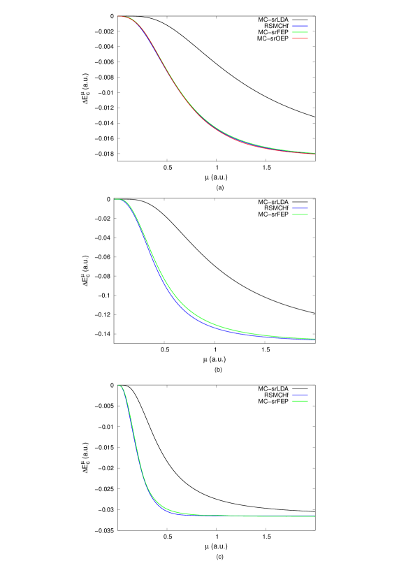
Figure 1: The quantity $\Delta E_{\rm c}^{\mu}$ for (from top to bottom) H₂, N₂ and Li₂ for each method as a function of the parameter $\mu$. See text for further details.

For H₂, for example, the RSMCHf and MC-srLDA $\mu$ values are 0.25 and 0.5, respectively.

It is tempting to conclude that the prescription of Fromager et al. Fromager et al. (2007) leads to different optimal $\mu$ values when considering RSMCHf energies. The situation is more subtle, however. The $\Delta E_{\rm c}^{\mu}$ energy difference calculated within RSMCHf contains different correlation effects to the one obtained within the MC-srLDA scheme. In the latter case, $\Delta E_{\rm c}^{\mu}$ is essentially the purely long-range correlation energy while, within RSMCHf, it also contains the coupling between short- and long-range correlations that arises from the expectation value of the short-range interaction over the long-range correlated MC-srLDA wavefunction (see Eq. (29)). This appears clearly in range-separated second-order density-functional perturbation theory (DFPT2) where a long-range MP2 description is used rather than a MCSCF one.Cornaton et al. (2013) For small $\mu$ values, the difference between MC-srLDA and RSMCHf correlation energies can be rationalized by considering the Taylor expansions of the long- and short-range interactions,

$$w^{\rm lr,\mu}_{\rm ee}(r_{12}) =\frac{2}{\sqrt{\pi}}\left(\mu-\frac{1}{3}\mu^{3}r_{12}^{2}+\mathcal{O}(\mu^{5})\right),$$

$$w^{\rm sr,\mu}_{\rm ee}(r_{12}) =\frac{1}{r_{12}}+\mathcal{O}(\mu).$$ (61)

As the deviation of the exact long-range interacting wavefunction from the KS determinant varies as $\mu^{3}$ (see Appendix B4 of Ref. Toulouse et al., 2004a), the long-range correlation energy varies as $\mu^{6}$ and the coupling between long- and short-range correlations as $\mu^{3}$. As a result, the latter is expected to deviate more rapidly from zero as $\mu$ increases. This is the reason why a threshold of $-1mE_{h}$ on $\Delta E_{\rm c}^{\mu}$ will provide a smaller $\mu$ value for RSMCHf than for MC-srLDA. As shown in Fig. 1, the same conclusion can be drawn for MC-srFEP and MC-srOEP. This was expected as all three models use the same energy expression. They only differ by the long-range MC wavefunction that is inserted into this expression for the computation of the energy. If we want to follow the prescription of Fromager et al.,  Fromager et al. (2007) which relies on the analysis of purely long-range correlation effects, one should extract from $\Delta E_{\rm c}^{\mu}$ the purely long-range correlation energy or increase the threshold. As this analysis is performed on static-correlation free electronic systems, range-separated DFPT2 Cornaton et al. (2013) is expected to be a good approximation to RSMCHf, especially for small $\mu$ values. In this context, the coupling between long- and short-range correlations can be separated from the purely long-range correlation energy and each term can be computed when varying $\mu$. Results obtained for rare gas atoms are presented in Ref. Cornaton et al., 2013. When $\mu=0.4$, the coupling term equals -4 and -20 $mE_{h}$ in He and Ne, respectively, while the long-range correlation energy is above -1 $mE_{h}$ in both systems. This suggests that the coupling term is more system-dependent than the purely long-range correlation energy. It was expected as the former is expressed in terms of both long- and short-range integrals. In order to reduce the system-dependency of the $\mu$ parameter, one may want to examine purely long-range correlation effects only, leading thus to the optimal $\mu=0.4$ value for the rare gas atoms Cornaton et al. (2013).

Returning to H₂ and the RSMCHf model, we can still utilize, as an alternative, the second strategy of Ref. Fromager et al., 2007 that relies on the analysis of the natural orbital occupancies as $\mu$ increases from zero. Since RSMCHf and MC-srLDA wavefunctions are identical by definition, we can simply refer to Ref. Fromager et al., 2007 and conclude that $\mu=0.4$ is also optimal in this context. This is illustrated by the MC-srLDA occupancies of H₂ in Fig. 2. Interestingly, similar conclusions can be drawn for H₂ at both MC-srFEP and MC-srOEP levels. This should clearly be investigated on more static-correlation-free systems, once the analytical MC-srOEP energy gradient is implemented. This is left for future work. Note that $\mu=0.4$ is large enough to assign static correlation in Li₂ and N₂, or at least a part of it, to the long-range MCSCF as suggested by their natural orbital occupancies in Fig. 2.

In summary, our preliminary calculations suggest that it is relevant to use $\mu=0.4$ in conjunction with the alternative separation of exchange and correlation energies of Toulouse et al.Toulouse et al. (2005a)

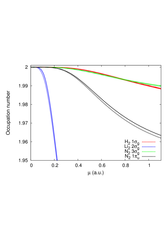
Figure 2: Occupation numbers of MC-srLDA (dotted), MC-srFEP (dashed) and MC-srOEP (solid) active natural orbitals as a function of $\mu$ for H₂, N₂ and Li₂ at their experimental equilibrium geometries Lie and Clementi (1974a, b); Coxon and Melville (2006); Barakat et al. (1986).

IV.2 Potential curves of H₂, N₂, Li₂ and H₂O

IV.2.1 RSMCHf equilibrium distances and binding energies

In this section, we compare the performance of the RSMCHf and MC-srLDA schemes for the description of the potential energy curves (PECs) of H₂, N₂, Li₂ and H₂O. In the latter case, the symmetric dissociation at the experimental equilibrium angle H–O–H of 104.5^∘ Hasted (1972) was investigated. PECs as well as equilibrium bond distances and dissociation energies are given in Fig. 3 and Tables 2 and 3, respectively. According to Sec. IV.1 the $\mu$ parameter has been set to 0.4.

For the H₂ molecule, close to the equilibrium geometry, MC-srLDA has a total energy that is too positive, though it recovers more short-range dynamical correlation than standard MCSCF. Although the qualitative shape of the curve is much better than restricted Hartree–Fock (not shown), the energy in the dissociation regime is much too positive. Overall this leads to a dissociation energy which is much too large, as shown in Table 2. The RSMCHf approach gives energies close to equilibrium that are slightly too negative, whilst those at dissociation are significantly too negative. The result is a slight underestimation of the dissociation energy. The deviations from the exact curve in the dissociation regime come from the complementary MD srLDA correlation functional, as illustrated by the RSMCHf (no src) PEC in Fig. 3, obtained when subtracting the former from the RSMCHf energy. As expected, the RSMCHf (no src) energy, which is equal to the expectation value of the regular Hamiltonian over the MC-srLDA wavefunction, is greater than the pure MCSCF energy for all bond distances.

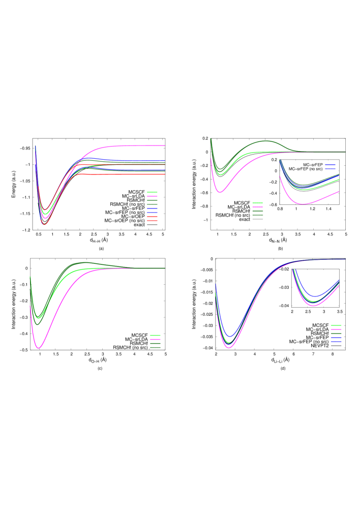
Figure 3: Potential energy curves (a. u.) of H₂ (upper left panel) and interaction (binding) energies of N₂ (upper right panel), H₂O (lower left panel) and Li₂ (lower right panel) obtained by means of the new multi-configuration range-separated schemes. The coupling parameter is $\mu$=0.4. The exact interaction energy and PEC curves are taken from Ref. Lie and Clementi, 1974b for H₂ and Ref. Lie and Clementi, 1974a for N₂.

Returning to the equilibrium distance, the too negative MD srLDA correlation energy for H₂ at $\mu=0.4$ was already observed by Gori-Giorgi and Savin (see the uppermost panel in Fig. 7 of Ref. Gori-Giorgi and Savin, 2009), who obtained an error (about 0.01$E_{\text{h}}$ in absolute value) close to that at the RSMCHf level (0.007$E_{\text{h}}$) when comparing with the “exact” energy of Ref. Lie and Clementi, 1974b. In spite of these errors, the RSMCHf model clearly improves upon the dissociation energy obtained at the MC-srLDA level, reducing the absolute error from 27 to 7% for H₂, with similar conclusions for the other systems.

The calculated equilibrium bond distances compare relatively well with experiment at both MC-srLDA and RSMCHf levels (see Table 2). While the MC-srLDA model slightly overestimates the bond distance of H₂ by 0.015 Å, the RSMCHf model underestimates it by 0.02 Å. This slight over-binding is induced by the complementary MD srLDA correlation functional, as suggested by the RSMCHf (no src) equilibrium distance of 0.744 Å, which is almost equal to the experimental value. Note that MC-srLDA and HF-srLDA bond distances are almost identical since, for $\mu=0.4$, the MC-srLDA wave function is well approximated by a single determinant (see Sec. IV.1 and Fig. 4).

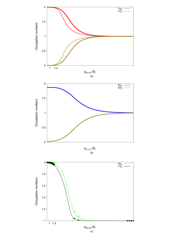
Figure 4: Occupation numbers of MC-srOEP (solid), MC-srFEP (dotted) and MC-srLDA (dashed) active natural orbitals as a function of bond distance (Å) (from top to bottom) H₂, Li₂ and N₂. The parameter $\mu$ is set to 0.4.

On the other hand, RSHf and RSMCHf equilibrium distances are quite similar but not as close as HF-srLDA and MC-srLDA distances (see Table 2). The (slight) difference may be caused by the short/long-range correlation coupling, which contributes significantly to the RSMCHf correlation energy, where it is treated explicitly within the MCSCF, unlike for the MC-srLDA energy, where it is described within DFT (see Sec. IV.1). Similar conclusions can be drawn for the other systems when comparing MC-srLDA with RSMCHf equilibrium distances, as shown in Tables 2 and 3.

IV.2.2 The treatment of static correlation within RSMCHf

Regarding the H₂ dissociation limit, the large error in the MC-srLDA energy was interpreted in Ref. Fromager et al., 2007 as a self-interaction error of the complementary spin-unpolarised srLDA exchange–correlation functional. We emphasize that the complementary short-range correlation energy, whose exact expression is given in Eq. (18), is not supposed to be zero at large internuclear distances—instead, it should compensate the short-range Hartree and exchange energy contributions. This was shown by Teale et al.,Teale et al. (2010) who computed accurately the correlation integrand in Eq. (II.2) for various bond distances. According to Eq. (18), the accurate short-range correlation energy is obtained for $\mu=0.4$ when integrating the correlation integrand in Fig. 6 (f) of Ref. Teale et al., 2010 from $\mu/(1+\mu)=0.286$ to 1. This quantity is obviously not equal to zero. The sum of short-range Hartree, exchange and correlation energies should, on the other hand, vanish in the dissociation limit. The corresponding integrand in Eq. (7) is plotted in Fig. 6 (d) of Ref. Teale et al., 2010. Pure short-range exchange–correlation density functionals like srLDA are simply unable to compensate the short-range Hartree term. Fromager et al. (2007)

The error in the total energy at large distances is significantly reduced when using the RSMCHf model, based on a different decomposition of the short-range exchange–correlation energy. The complementary short-range MD density-functional correlation energy is defined, in RSMCHf, with respect to the long-range interacting wavefunction rather than the KS non-interacting one. Its exact expression is given in Eq. (25) in terms of the short-range MD correlation integrand of Eq. (II.3). Since the long-range wavefunction in the dissociation limit of H₂ reduces to the Heitler–London wavefunction for all non-zero $\mu$ values,Gori-Giorgi and Savin (2009) this integrand and, consequently, the short-range MD correlation energy should vanish upon bond stretching. This is an important difference between MC-srDFT and RSMCHf schemes. While the former is expected to describe much of the static correlation with the short-range correlation functional, the latter treats all static correlation with MCSCF, at least in the dissociation limit.

Comparing the RSMCHf and RSMCHf (no src) PECs of H₂ at large separations, it is clear that the short-range MD correlation energy is not well described within the local density approximation, as expected from the work of Gori-Giorgi and Savin.Gori-Giorgi and Savin (2009) The error can be interpreted as a self-correlation error of the spin-unpolarized MD srLDA functional since the molecule is correctly dissociated into two neutral hydrogen atoms (see the MC-srLDA natural orbital occupancies in Fig. 4). It is, however, not exclusively due to the functional—indeed, the RSMCHf (no src) PEC deviates slightly from the exact PEC. The deviation comes from the MC-srLDA wavefunction that is used to compute the RSMCHf (no src) energy. The former contains self-interaction errors because of the srLDA exchange–correlation density-functional potential. This problem will be addressed in the following sections.

Finally, we observe for H₂ a slight bump in the intermediate region ($R=2.25$ Å) of the RSMCHf PEC. It is even more pronounced for H₂O and N₂. No bump appears for Li₂, possibly because (unlike the other systems) it has a significant multi-configuration character already at equilibrium (see Fig. 4). Interestingly, at $R=2.117$ Å, the RSMCHf (no src) energy of H₂ deviates from the exact one by about 0.03 $E_{\text{h}}$, which could be interpreted as the correct value for the short-range MD correlation energy (the RSMCHf energy is relatively close to the exact one). However, from the srOEP calculations of Gori-Giorgi and Savin (the lowest panel in Fig. 7 of Ref. Gori-Giorgi and Savin, 2009), the accurate value of this energy for $\mu=0.4$ is 0.01–0.015 $E_{\text{h}}$. This difference suggests that the srLDA exchange–correlation density-functional potential, from which the MC-srLDA wavefunction (and hence the RSMCHf energy) is obtained, may not be accurate enough, especially as the wavefunction is strongly multi-configurational in this region, as shown in Fig. 4. Interestingly, errors on the short-range potential and the short-range MD correlation density functional seem to compensate in the RSMCHf energy when $R=2.117$ Å but not for the other bond distances. Use of srOEPs rather than srLDA potentials is then a reasonable alternative, as is investigated in the following.

IV.2.3 MC-srFEP results

The MC-srFEP model that was introduced in Sec. II.6 corresponds to a zero-iteration MC-srOEP calculation where the long-range MC wavefunction only is optimized. The initial HF-srOEP potential is simply frozen. Equilibrium bond distances and binding energies obtained at the MC-srFEP level are given in Tables 2 and 3. Full PECs have been plotted in Fig. 3 for H₂ and Li₂. Convergence problems in the HF-srOEP calculation occurred for 1.6 $\leq R\leq$ 3.5 Å in N₂ and for all O–H distances beyond 2.0 Å in H₂O—that is, when the long-range wavefunction becomes strongly multi-configurational, as shown in Fig. 4. In these cases, we expect the convergence of the srOEP to be manageable only at the long-range MCSCF level, requiring the implementation of analytical gradients, which is currently in progress.

For H₂ and Li₂, we observe that the MC-srFEP and RSMCHf PECs remain relatively close for all bond distances, the natural orbital occupations being almost identical (see Fig. 4). For H₂ at equilibrium, the MC-srFEP energy is slightly lower than the RSMCHf energy, meaning that the HF-srOEP potential is better than the srLDA one, according to the variational principle in Eq. (42). However, as the bond is stretched and the wavefunction becomes multi-configurational, the MC-srFEP energy becomes higher than the RSMCHf one. This is expected since the HF-srOEP potential is unaffected by long-range correlation. For comparison, the MC-srFEP (no src) PEC has been computed. In this case the frozen potential is calculated at the HF-srOEP (no src) level, that is without the MD srLDA correlation term. In the dissociation limit, the MC-srFEP (no src) energy is too high which clearly indicates that the HF-srOEP (no src) potential is a poor approximation to the exact short-range potential. Optimization of the srOEP at the long-range MCSCF level should, on the other hand, give essentially the exact solution.Gori-Giorgi and Savin (2009) It is noteworthy that, in a minimal atomic-orbital basis, the exact energy would actually be obtained at both RSMCHf (no src) and MC-srFEP (no src) levels of theory since the wavefunction is then fixed to $1/\sqrt{2}\left(|1\sigma_{g}^{2}\rangle-|1\sigma_{u}^{2}\rangle\right)$, where the bonding $1\sigma_{g}$ and the anti-bonding $1\sigma_{u}$ molecular orbitals are simply linear combinations of the atomic $1s$ orbitals of each hydrogen atom.Sharkas et al. (2012) In our calculations, as larger basis are used, orbitals can rotate so that different energies can be obtained.

Returning to RSMCHf, the srLDA density-functional potential, even though it may be a crude approximation to the exact potential, includes multi-configuration effects through the density. It is therefore more accurate than the HF-srOEP potential. Note also that, in the intermediate region, the maximum of the bump is at a higher energy with the MC-srFEP model than with the RSMCHf model. In conclusion, MC-srFEP provides better binding energies than RSMCHf but this essentially relies on error compensation.

IV.2.4 MC-srOEP results for H₂

We now consider the calculation of the PEC of H₂ at the MC-srOEP level. For comparison, the MC-srOEP (no src) PEC was also calculated. These PECs are shown in Fig. 3. As expected, the MC-srOEP and MC-srFEP PECs are almost identical in the equilibrium region where static correlation is negligible. As in the MC-srLDA scheme, the MC-srOEP wavefunction is essentially a single determinant (see Fig. 4).

Upon bond stretching, the MC-srOEP PEC deviates from the MC-srFEP curve. Interestingly, the separation occurs when the MC-srFEP energy is higher than the RSMCHf one, that is when the HF-srOEP potential becomes less accurate than the srLDA one, as discussed previously. The difference between MC-srOEP and MC-srFEP energies is reflected both in the orbital occupations and in the orbitals (not shown). The MC-srOEP wavefunction has a much more pronounced multi-configurational character than the MC-srFEP wavefunction, as shown in Fig. 4. This explains why the MC-srOEP energy reaches it asymptotic limit at a shorter bond distance ($R\approx 2.2$ Å) than does the MC-srFEP energy ($R\approx 3.5$ Å). As expected, the exact energy is recovered at the MC-srOEP (no src) level in the dissociation limit. Due to self-correlation errors in the MD srLDA functional, the MC-srOEP energy is too low at the dissociation. This leads to an underestimation of the binding energy, which is actually even more pronounced than for RSMCHf and MC-srFEP.

In the intermediate region, at $R=2.117$ Å, the MC-srOEP (no src) energy differs from the exact one by 0.017$E_{\text{h}}$, as expected for the accurate short-range MD correlation energy from the work of Gori-Giorgi and Savin.Gori-Giorgi and Savin (2009) The MD srLDA correlation energy obtained by us ($-0.03E_{\text{h}}$) agrees perfectly with their value, see the lowest panel in Fig. 7 of Ref. Gori-Giorgi and Savin, 2009. Note also that the bump observed at the RSMCHf and MC-srFEP levels is significantly reduced at the MC-srOEP level but not completely removed.

In conclusion, our preliminary MC-srOEP calculations on H₂ confirm that the MD srLDA correlation functional of Paziani et al. Paziani et al. (2006) can be improved upon. The conclusion is basically the same as for MC-srLDA: better short-range functionals should be developed. However, the exact complementary short-range correlation energy to be modelled (namely the MD one) is supposed to vanish in the dissociation limit, unlike the KS short-range correlation energy that is used in conventional MC-srDFT models. It may therefore be easier to develop better short-range MD correlation density functionals. The ab initio calculation of the range-separated adiabatic connection Teale et al. (2010) is a valuable tool for such developments.

IV.2.5 Analysis of the srOEPs

When applying the OEP method care must be taken to ensure that smooth potentials are obtained. In the present work we have used uncontracted basis sets and chosen the orbital and potential sets identical to help ensure this is the case. In Fig. 5 we present the exchange–correlation contributions to the HF-srOEP potentials. For this figure we have generated the potentials using the smoothing-norm approach of Heaton-Burgess et al.Heaton-Burgess et al. (2007); Heaton-Burgess and Yang (2008) with a smoothing parameter of $10^{-5}$. This value perturbs the energy by less than $10^{-5}$a.u. from the unconstrained energies presented in the rest of this work. The result is a a potential that is everywhere smooth. Without the application of this approach the potential very close to the nuclei exhibits a large spike, owing to the fact that this region has essentially no contribution when determining the energy of the system. The potential in other regions of space is essentially unchanged from its unconstrained counterpart.

In the top panel of Fig. 5 the potentials exhibit relatively few features, although as $\mu$ increases the positions of the nuclei can be discerned. As would be expected the from the discussion in Sec. II the srOEP potential approaches zero as the value of $\mu$ is increased. The other feature of the potentials that is clearly visible is their rate of decay as a function of $\mu$. For $\mu=0.00$ a KS-OEP is obtained and exhibits the usual $-1/r$ asymptotic decay. As mu is increased the decay of the potential becomes more rapid, reflecting the form of Eq. (44). For $\mu=0.4$ the potential contributions along the bond axis are essentially zero beyond approximately $5$ a.u. from each atom. Interestingly, the potential near the atoms is also affected rather strongly by the change in $\mu$, this may again reflect the inclusion of long-range / short-range coupling effects in the partitioning of Toulouse et al. Toulouse et al. (2005a). For the longer bond lengths in the lower two panels of Fig. 5 similar conclusions can be reached, though as the atoms are further separated their positions become clearer in the associated potentials.

For the MC-srOEP approach the exchange–correlation potentials obtained (not shown) are very similar, having only very slightly more negative potentials surrounding the nuclei and slightly more positive potentials further away in the intermediate “shoulder” regions. Whilst these subtle changes are essential for proper optimization of the MC-srOEP energy, they do not significantly alter the potentials from those of the HF-srOEP approach on the scale shown.

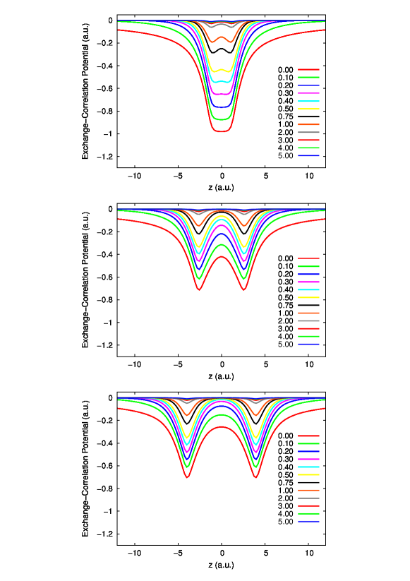
Figure 5: The exchange–correlation contributions to the srOEPs plotted along the bond axis for the H₂ molecule at the HF-srOEP level. The top panel corresponds to $R=1.3$Å, the middle to $R=2.8$Åand the bottom to $R=4.2$Å. In each panel the potentials are shown for $\mu=0.00,0.10,0.20,0.30,0.40,0.50,0.75,1.00,2.00,3.00,4.00,5.00$ and these may be distinguished by noting that the potential value at $z=0.0$ increases with increasing $\mu$.

V Conclusions

An alternative separation of exchange and correlation energies has been investigated in the context of multi-configuration range-separated DFT. The new decomposition of the short-range exchange–correlation energy relies on the auxiliary long-range interacting wavefunction rather than the KS determinant. This approach, first proposed by Toulouse et al.,Toulouse et al. (2005a) has two advantages relative to the traditional KS decomposition. First, the MCSCF part of the energy is now computed with the regular (fully-interacting) Hamiltonian, following CAS-DFT approaches.Gräffenstein and Cremer (2000); Gusarov et al. (2004) Second, the exact complementary short-range correlation energy vanishes upon dissociation of H₂, meaning that the static correlation is fully assigned to MCSCF.

The drawback is that, because of double counting, the long-range interacting wave function used to compute the energy cannot be obtained by minimizing the energy expression with respect to the wavefunction parameters. Different approaches that overcome this problem have been investigated. The first simply computes the energy from the long-range interacting MCSCF wavefunction that is optimized with the traditional KS decomposition of the short-range density-functional energy. A more sophisticated scheme uses short-range OEPs. The resulting combination of OEP techniques with wavefunction theory has been investigated in this work, at the HF and MCSCF levels.

In the HF case, an analytical expression for the energy gradient has been derived and implemented. Calculations have been performed within the short-range local density approximation on H₂, N₂, Li₂ and H₂O. Significant improvements in binding energies are obtained with the new decomposition of the short-range energy, relative to the traditional one. The importance of optimizing the short-range OEP at the MCSCF level when static correlation becomes significant has been demonstrated for H₂, using a finite-difference gradient. For further assessment of this approach, the analytical gradient is under implementation.

Our preliminary calculations indicate that the local density approximation is not accurate enough for modelling the complementary short-range correlation energy—better functionals may be developed from an accurate calculation of range-separated adiabatic-connection paths. Work is in progress in this direction.

Appendix: HF-srOEP linear response equation

The response of the HF-srOEP determinant related to variations $\epsilon_{t}$ in the srOEP coefficients is obtained when considering the auxiliary energy

$$\mathcal{E}^{\mu}({\boldsymbol{\kappa}},\epsilon_{t}) =\langle\Phi({\boldsymbol{\kappa}})|\hat{T}+\hat{W}^{\rm lr,\mu}_{\rm ee}+\hat{V_{0}}|\Phi({\boldsymbol{\kappa}})\rangle$$

$$+\sum_{t}\epsilon_{t}\langle\Phi({\boldsymbol{\kappa}})|\hat{g}_{t}|\Phi({\boldsymbol{\kappa}})\rangle$$

$$=\mathcal{E}^{\mu}({\boldsymbol{\kappa}})+\sum_{t}\epsilon_{t}\langle\Phi({\boldsymbol{\kappa}})|\hat{g}_{t}|\Phi({\boldsymbol{\kappa}})\rangle,$$ (62)

where $\hat{V_{0}}=\int{\rm d}{\mathbf{r}}\;v_{0}({\mathbf{r}})\,\hat{n}({\bf r})$ is the trial srOEP and the Gaussian operator $\hat{g}_{t}=\int{\rm d}{\mathbf{r}}\;g_{t}({\mathbf{r}})\,\hat{n}({\bf r})$ is analogous to a property operator in response theory Salek et al. (2005). From the variational condition in Eq. (39) we obtain

$$\forall\epsilon_{t}\hskip 8.5359pt{\left.\frac{\partial\mathcal{E}^{\mu}({\boldsymbol{\kappa}},\epsilon_{t})}{\partial{\boldsymbol{\kappa}}}\right|_{{\boldsymbol{\kappa}}(\epsilon_{t})}=0},$$ (63)

which leads to the linear response equation

$$\left.\frac{\rm d}{\rm d\epsilon_{t}}\left(\frac{\partial\mathcal{E}^{\mu}({\boldsymbol{\kappa}},\epsilon_{t})}{\partial{\boldsymbol{\kappa}}}\right)\right|_{0}=0.$$ (64)

Using the Taylor expansion through second order

$$\mathcal{E}^{\mu}({\boldsymbol{\kappa}})=\mathcal{E}^{\mu}(0)+{\frac{1}{2}{\boldsymbol{\kappa}}^{\rm T}\mathcal{E}^{[2]\mu}\hskip 2.84544pt{\boldsymbol{\kappa}}+\ldots,}$$ (65)

where the HF-type Hessian $\mathcal{E}^{[2]\mu}$ is constructed from the auxiliary long-range interacting Hamiltonian $\hat{T}+\hat{W}^{\rm lr,\mu}_{\rm ee}+\hat{V_{0}}$, and rewriting the first-order derivative of the Gaussian expectation value as Helgaker et al. (2004)

$$\left.\frac{\partial}{\partial{\boldsymbol{\kappa}}}\langle\Phi({\boldsymbol{\kappa}})|\hat{g}_{t}|\Phi({\boldsymbol{\kappa}})\rangle\right|_{0}=g_{t}^{[1]},$$ (66)

where the gradient Gaussian vector expression is given in Eq. (54), we finally obtain Eq. (53).

TABLE CAPTION

Table 1

Wavefunction, local potential and energy expressions associated with all range-separated methods discussed in this work. Single determinantal trial wavefunctions are denoted $\Phi$. $\hat{H}=\hat{T}+\hat{W}_{\rm ee}+\hat{V}_{\rm ne}$ and $\hat{H}^{\rm lr,\mu}=\hat{T}+\hat{W}^{\rm lr,\mu}_{\rm ee}+\hat{V}_{\rm ne}$ correspond to the physical (fully interacting) and long-range interacting Hamiltonians, respectively. $S_{M}$ denotes the active space used in the long-range MCSCF calculation.

Table 2

Equilibrium bond distances R_e (Å) and binding energies D_e (eV) for the ground state of H₂ and N₂. The $\mu$ parameter was set to 0.4. See text for further details.

Table 3

Equilibrium bond distances R_e (Å) and binding energies D_e (eV) for the ground state of Li₂ and of H₂O at fixed H-O-H angle of 104.5^∘. The $\mu$ parameter was set to 0.4. See text for further details.

FIGURE CAPTIONS

Figure 1

The quantity $\Delta E_{\rm c}^{\mu}$ for (from top to bottom) H₂, N₂ and Li₂ for each method as a function of the parameter $\mu$. See text for further details.

Figure 2

Occupation numbers of MC-srLDA (dotted), MC-srFEP (dashed) and MC-srOEP (solid) active natural orbitals as a function of $\mu$ for H₂, N₂ and Li₂ at their experimental equilibrium geometries Lie and Clementi (1974a, b); Coxon and Melville (2006); Barakat et al. (1986).

Figure 3

Potential energy curves (a. u.) of H₂ (upper left panel) and interaction (binding) energies of N₂ (upper right panel), H₂O (lower left panel) and Li₂ (lower right panel) obtained by means of the new multi-configuration range-separated schemes. The range separation parameter is $\mu$=0.4. The exact interaction energy and PEC curves are taken from Ref. Lie and Clementi, 1974b for H₂ and Ref. Lie and Clementi, 1974a for N₂.

Figure 4

Occupation numbers of MC-srLDA (dashed), MC-srFEP (dotted) and MC-srOEP (solid) active natural orbitals as a function of bond distance (Å) (from top to bottom) H₂, Li₂ and N₂  Lie and Clementi (1974a, b); Coxon and Melville (2006); Barakat et al. (1986). The parameter $\mu$ is set to 0.4.

Figure 5

The exchange–correlation contributions to the srOEPs plotted along the bond axis for the H₂ molecule at the HF-srOEP level. The top panel corresponds to $R=1.3$Å, the middle to $R=2.8$Å and the bottom to $R=4.2$Å. In each panel the potentials are shown for $\mu=0.00,0.10,0.20,0.30,0.40,0.50,0.75,1.00,2.00,3.00,4.00,5.00$ and these may be distinguished by noting that the potential value at $z=0.0$ increases with increasing $\mu$.

Table 1: Stoyanova et al., Journal of Chemical Physics

method			wavefunction		local potential		energy expression
HF-srLDA			$\Phi^{\mu}=\!\operatorname*{arg\,min}\limits_{\Phi}\!\Big{\{}\!\langle\Phi|\hat{H}^{\rm lr,\mu}|\Phi\rangle$		$v_{\rm ne}({\bf r})+\delta E^{\rm sr,\mu}_{\rm Hxc}/\delta n({\bf r})[n_{\Phi^{\mu}}]$		$\langle\Phi^{\mu}|\hat{H}^{\rm lr,\mu}|\Phi^{\mu}\rangle+E^{\rm sr,\mu}_{\rm Hxc}[n_{\Phi^{\mu}}]$
			$+E^{\rm sr,\mu}_{\rm Hxc}[n_{\Phi}]\Big{\}}$
MC-srLDA			$\Psi_{M}^{\mu}=\!\operatorname*{arg\,min}\limits_{\Psi\in S_{M}}\!\Big{\{}\!\langle\Psi|\hat{H}^{\rm lr,\mu}|\Psi\rangle$		$v_{\rm ne}({\bf r})+\delta E^{\rm sr,\mu}_{\rm Hxc}/\delta n({\bf r})[n_{\Psi_{M}^{\mu}}]$		$\langle\Psi_{M}^{\mu}|\hat{H}^{\rm lr,\mu}|\Psi_{M}^{\mu}\rangle+E^{\rm sr,\mu}_{\rm Hxc}[n_{\Psi_{M}^{\mu}}]$
			$+E^{\rm sr,\mu}_{\rm Hxc}[n_{\Psi}]\Big{\}}$
RSHf			$\Phi^{\mu}$ [HF-srLDA]		$v_{\rm ne}({\bf r})+\delta E^{\rm sr,\mu}_{\rm Hxc}/\delta n({\bf r})[n_{\Phi^{\mu}}]$		$\langle\Phi^{\mu}|\hat{H}|\Phi^{\mu}\rangle+E^{\rm sr,\mu}_{\rm c,md}[n_{\Phi^{\mu}}]$
RSMCHf			$\Psi_{M}^{\mu}$ [MC-srLDA]		$v_{\rm ne}({\bf r})+\delta E^{\rm sr,\mu}_{\rm Hxc}/\delta n({\bf r})[n_{\Psi_{M}^{\mu}}]$		$\langle\Psi_{M}^{\mu}|\hat{H}|\Psi_{M}^{\mu}\rangle+E^{\rm sr,\mu}_{\rm c,md}[n_{\Psi_{M}^{\mu}}]$
RSMCHf (no src)			$\Psi_{M}^{\mu}$ [MC-srLDA]		$v_{\rm ne}({\bf r})+\delta E^{\rm sr,\mu}_{\rm Hxc}/\delta n({\bf r})[n_{\Psi_{M}^{\mu}}]$		$\langle\Psi_{M}^{\mu}|\hat{H}|\Psi_{M}^{\mu}\rangle$
HF-srOEP			$\Phi^{\mu}[v_{1}^{\mu}]$		$v_{1}^{\mu}=\!\operatorname*{arg\,min}\limits_{v}\!\Big{\{}\!\langle\Phi^{\mu}[v]|\hat{H}|\Phi^{\mu}[v]\rangle$		$\langle\Phi^{\mu}[v_{1}^{\mu}]|\hat{H}|\Phi^{\mu}[v_{1}^{\mu}]\rangle+E^{\rm sr,\mu}_{\rm c,md}[n_{\Phi^{\mu}[v_{1}^{\mu}]}]$
					$+E^{\rm sr,\mu}_{\rm c,md}[n_{\Phi^{\mu}[v]}]\Big{\}},$
					$\Phi^{\mu}[v]=\!\operatorname*{arg\,min}\limits_{\Phi}\!\Big{\{}\!\langle\Phi|\hat{T}+\hat{W}^{\rm lr,\mu}_{\rm ee}|\Phi\rangle$
					$+\!\!\int\!\!{\rm d}{\mathbf{r}}\,v({\mathbf{r}}){n}_{\Phi}({\bf r})\!\Big{\}}$
HF-srOEP (no src)			$\Phi^{\mu}[v_{2}^{\mu}]$		$v_{2}^{\mu}=\!\operatorname*{arg\,min}\limits_{v}\!\Big{\{}\!\langle\Phi^{\mu}[v]|\hat{H}|\Phi^{\mu}[v]\rangle\Big{\}}$		$\langle\Phi^{\mu}[v_{2}^{\mu}]|\hat{H}|\Phi^{\mu}[v_{2}^{\mu}]\rangle$
MC-srFEP			$\Psi_{M}^{\mu}[v_{1}^{\mu}]=\!\operatorname*{arg\,min}\limits_{\Psi\in S_{M}}\!\Big{\{}\!\langle\Psi|\hat{T}+\hat{W}^{\rm lr,\mu}_{\rm ee}|\Psi\rangle$		$v_{1}^{\mu}$ [HF-srOEP]		$\langle\Psi_{M}^{\mu}[v_{1}^{\mu}]|\hat{H}|\Psi_{M}^{\mu}[v_{1}^{\mu}]\rangle+E^{\rm sr,\mu}_{\rm c,md}[n_{\Psi_{M}^{\mu}[v_{1}^{\mu}]}]$
			$+\!\!\int\!\!{\rm d}{\mathbf{r}}\,v^{\mu}_{1}({\mathbf{r}}){n}_{\Psi}({\bf r})\!\Big{\}}$
MC-srFEP (no src)			$\Psi_{M}^{\mu}[v_{2}^{\mu}]=\!\operatorname*{arg\,min}\limits_{\Psi\in S_{M}}\!\Big{\{}\!\langle\Psi|\hat{T}+\hat{W}^{\rm lr,\mu}_{\rm ee}|\Psi\rangle$		$v_{2}^{\mu}$ [HF-srOEP (no src)]		$\langle\Psi_{M}^{\mu}[v_{2}^{\mu}]|\hat{H}|\Psi_{M}^{\mu}[v_{2}^{\mu}]\rangle$
			$+\!\!\int\!\!{\rm d}{\mathbf{r}}\,v^{\mu}_{2}({\mathbf{r}}){n}_{\Psi}({\bf r})\!\Big{\}}$
MC-srOEP			$\Psi_{M}^{\mu}[v_{3}^{\mu}]$		$v_{3}^{\mu}=\!\operatorname*{arg\,min}\limits_{v}\!\Big{\{}\!\langle\Psi_{M}^{\mu}[v]|\hat{H}|\Psi_{M}^{\mu}[v]\rangle$		$\langle\Psi_{M}^{\mu}[v_{3}^{\mu}]|\hat{H}|\Psi_{M}^{\mu}[v_{3}^{\mu}]\rangle+E^{\rm sr,\mu}_{\rm c,md}[n_{\Psi_{M}^{\mu}[v_{3}^{\mu}]}]$
					$+E^{\rm sr,\mu}_{\rm c,md}[n_{\Psi_{M}^{\mu}[v]}]\Big{\}},$
					$\Psi_{M}^{\mu}[v]=\!\operatorname*{arg\,min}\limits_{\Psi\in S_{M}}\!\Big{\{}\!\langle\Psi|\hat{T}+\hat{W}^{\rm lr,\mu}_{\rm ee}|\Psi\rangle$
					$+\!\!\int\!\!{\rm d}{\mathbf{r}}\,v({\mathbf{r}}){n}_{\Psi}({\bf r})\!\Big{\}}$
MC-srOEP (no src)			$\Psi_{M}^{\mu}[v_{4}^{\mu}]$		$v_{4}^{\mu}=\!\operatorname*{arg\,min}\limits_{v}\!\Big{\{}\!\langle\Psi_{M}^{\mu}[v]|\hat{H}|\Psi_{M}^{\mu}[v]\rangle\Big{\}}$		$\langle\Psi_{M}^{\mu}[v_{4}^{\mu}]|\hat{H}|\Psi_{M}^{\mu}[v_{4}^{\mu}]\rangle$

Table 2: Stoyanova et al., Journal of Chemical Physics

	Re	De
H2
HF-srLDA	0.755	10.39
RSHf	0.717	11.73
HF-srOEP	0.715	11.75
MCSCF	0.755	4.14
MC-srLDA	0.756	6.05
RSMCHf	0.724	4.41
RSMCHf (no src)	0.744	3.91
MC-srFEP	0.720	4.53
MC-srFEP (no src)	0.743	4.09
MC-srOEP	0.722	4.18
MC-srOEP (no src)	0.743	3.77
Exp.	0.741a	4.75a
N2
HF-srLDA	1.082	30.85
RSHf	1.051	36.86
HF-srOEP	1.052	34.55
MCSCF	1.105	9.19
MC-srLDA	1.087	16.18
RSMCHf	1.079	7.96
RSMCHf (no src)	1.096	6.86
MC-srFEP	1.077	8.34
MC-srFEP (no src)	1.095	7.44
Exp.	1.097a	9.91a

^aRef. Lie and Clementi, 1974a

Table 3: Stoyanova et al., Journal of Chemical Physics

	Re	De
Li2
HF-srLDA	2.671	3.273
RSHf	2.722	3.130
HF-srOEP	2.722	3.126
MCSCF	2.720b	1.029b
MC-srLDA	2.679	1.091
RSMCHf	2.669	1.039
RSMCHf (no src)	2.750	0.936
MC-srFEP	2.666	1.047
MC-srFEP (no src)	2.735	0.951
Exp.	2.673c	1.056c
H2O
HF-srLDA	0.961	19.29
RSHf	0.925	19.30
HF-srOEP	0.925	-
MCSCF	0.963	8.31
MC-srLDA	0.962	13.32
RSMCHf	0.926	9.40
RSMCHf (no src)	0.942	8.10
MC-srFEP	0.927	-
MC-srFEP (no src)	0.944	-
Exp.	0.957d	10.06e

^bNEVPT2: $R_{e}$ =2.720 Å,  $D_{e}$=1.043 eV, ^cRef. Coxon and Melville, 2006; Barakat et al., 1986, ^dRef. Hasted, 1972, ^eRef. Perdew et al., 1996

References

- Kohn and Sham (1965) W. Kohn and L. J. Sham, Phys. Rev. A 140, 1133 (1965).
- Malet and Gori-Giorgi (2012) F. Malet and P. Gori-Giorgi, Phys. Rev. Lett. 109, 246402 (2012).
- Becke (2013) A. D. Becke, J. Chem. Phys. 138, 074109 (2013).
- Schipper et al. (1998) P. R. T. Schipper, O. V. Gritsenko, and E. J. Baerends, Theor. Chem. Acc. 99, 329 (1998).
- Filatov and Shaik (1999) M. Filatov and S. Shaik, Chem. Phys. Lett. 304, 429 (1999).
- Chai (2012) J.-D. Chai, J. Chem. Phys. 136, 154104 (2012).
- Nygaard and Olsen (2013) C. R. Nygaard and J. Olsen, J. Chem. Phys. 138, 094109 (2013).
- Colle and Salvetti (1990) R. Colle and O. Salvetti, J. Chem. Phys. 93, 534 (1990).
- Savin (1988) A. Savin, Int. J. Quantum Chem. 34, 59 (1988).
- Savin (1989) A. Savin, J. Chem. Phys. 86, 757 (1989).
- Miehlich et al. (1997) B. Miehlich, H. Stoll, and A. Savin, Mol. Phys. 91, 527 (1997).
- Gräffenstein and Cremer (2000) J. Gräffenstein and D. Cremer, Chem. Phys. Lett. 316, 569 (2000).
- Stoll (2003) H. Stoll, Chem. Phys. Lett. 376, 141 (2003).
- Ying et al. (2012) F. Ying, P. Su, Z. Chen, S. Shaik, and W. Wu, J. Chem. Theory Comput. 8, 1608 (2012).
- Malcolm and McDouall (1998) N. O. J. Malcolm and J. J. W. McDouall, Chem. Phys. Lett. 282, 121 (1998).
- McDouall (2003) J. J. W. McDouall, Mol. Phys. 101, 361 (2003).
- Gräffenstein and Cremer (2005) J. Gräffenstein and D. Cremer, Mol. Phys. 103, 279 (2005).
- Gusarov et al. (2004) S. Gusarov, P.-Å. Malmqvist, R. Lindh, and B. O. Roos, Theor. Chem. Acc. 112, 84 (2004).
- Nakata et al. (2006) K. Nakata, T. Ukai, S. Yamanaka, T. Takada, and K. Yamaguchi, Int. J. Quantum Chem. 106, 3325 (2006).
- Yamanaka et al. (2006) S. Yamanaka, K. Nakata, T. Ukai, T. Takada, and K. Yamaguchi, Int. J. Quantum Chem. 106, 3312 (2006).
- Ukai et al. (2007) T. Ukai, K. Nakata, S. Yamanaka, T. Takada, and K. Yamaguchi, Mol. Phys. 105, 2667 (2007).
- Pérez-Jiménez and Pérez-Jordá (2007) A. J. Pérez-Jiménez and J. M. Pérez-Jordá, Phys. Rev. A 75, 012503 (2007).
- Weimer et al. (2008) M. Weimer, F. Della Sala, and A. Görling, J. Chem. Phys. 128, 144109 (2008).
- Kurzweil et al. (2009) Y. Kurzweil, K. V. Lawler, and M. Head-Gordon, Mol. Phys. 107, 2103 (2009).
- Savin (1996) A. Savin, Recent Developments and Applications of Modern Density Functional Theory (Elsevier Amsterdam, 1996), p. 327.
- Stoll and Savin (1985) H. Stoll and A. Savin, Density functional methods in physics (Plenum, New York, 1985), p. 177.
- Pedersen (2004) J. K. Pedersen, Ph.D. thesis, University of Southern Denmark (2004).
- Fromager et al. (2007) E. Fromager, J. Toulouse, and H. J. Aa. Jensen, J. Chem. Phys. 126, 074111 (2007).
- Fromager et al. (2009) E. Fromager, F. Réal, P. Wåhlin, U. Wahlgren, and H. J. Aa. Jensen, J. Chem. Phys. 131, 054107 (2009).
- Ángyán et al. (2005) J. G. Ángyán, I. C. Gerber, A. Savin, and J. Toulouse, Phys. Rev. A 72, 012510 (2005).
- Goll et al. (2005) E. Goll, H. J. Werner, and H. Stoll, Phys. Chem. Chem. Phys. 7, 3917 (2005).
- Toulouse et al. (2009) J. Toulouse, I. C. Gerber, G. Jansen, A. Savin, and J. G. Ángyán, Phys. Rev. Lett. 102, 096404 (2009).
- Fromager et al. (2010) E. Fromager, R. Cimiraglia, and H. J. Aa. Jensen, Phys. Rev. A 81, 024502 (2010).
- Janesko et al. (2009) B. G. Janesko, T. M. Henderson, and G. E. Scuseria, J. Chem. Phys. 130, 081105 (2009).
- Toulouse et al. (2011) J. Toulouse, W. Zhu, A. Savin, G. Jansen, and J. G. Ángyán, J. Chem. Phys. 135, 084119 (2011).
- Strømsheim et al. (2011) M. D. Strømsheim, N. Kumar, S. Coriani, E. Sagvolden, A. M. Teale, and T. Helgaker, J. Chem. Phys. 135, 194109 (2011).
- Teale et al. (2010) A. M. Teale, S. Coriani, and T. Helgaker, J. Chem. Phys. 133, 164112 (2010).
- Sharkas et al. (2012) K. Sharkas, A. Savin, H. J. Aa. Jensen, and J. Toulouse, J. Chem. Phys. 137, 044104 (2012).
- Toulouse et al. (2005a) J. Toulouse, P. Gori-Giorgi, and A. Savin, Theor. Chem. Acc. 114, 305 (2005a).
- Savin (1995) A. Savin, Recent advances in density functional methods (World Scientific, Singapore, 1995), vol. 1, pp. 129–153.
- Levy (1979) M. Levy, Proc. Natl. Acad. Sci. USA 76, 6062 (1979).
- Lieb (1983) E. H. Lieb, Int. J. Quantum Chem. 24, 243 (1983).
- Yang (1998) W. Yang, J. Chem. Phys. 109, 10107 (1998).
- Savin et al. (2003) A. Savin, F. Colonna, and R. Pollet, Int. J. Quantum Chem. 93, 166 (2003).
- Hohenberg and Kohn (1964) P. Hohenberg and W. Kohn, Phys. Rev. 136, B864 (1964).
- Toulouse et al. (2004a) J. Toulouse, F. Colonna, and A. Savin, Phys. Rev. A 70, 062505 (2004a).
- Toulouse and Savin (2006) J. Toulouse and A. Savin, J. Mol. Struct. (THEOCHEM) 762, 147 (2006).
- Toulouse et al. (2004b) J. Toulouse, A. Savin, and H. J. Flad, Int. J. Quantum Chem. 100, 1047 (2004b).
- Paziani et al. (2006) S. Paziani, S. Moroni, P. Gori-Giorgi, and G. B. Bachelet, Phys. Rev. B 73, 155111 (2006).
- Heyd et al. (2003) J. Heyd, G. E. Scuseria, and M. Ernzerhof, J. Chem. Phys. 118, 8207 (2003).
- Heyd and Scuseria (2004) J. Heyd and G. E. Scuseria, J. Chem. Phys. 120, 7274 (2004).
- Goll et al. (2006) E. Goll, H. J. Werner, H. Stoll, T. Leininger, P. Gori-Giorgi, and A. Savin, Chem. Phys. 329, 276 (2006).
- Toulouse et al. (2005b) J. Toulouse, F. Colonna, and A. Savin, J. Chem. Phys. 122, 014110 (2005b).
- Goll et al. (2009) E. Goll, M. Ernst, F. Moegle-Hofacker, and H. Stoll, J. Chem. Phys. 130, 234112 (2009).
- Gori-Giorgi and Savin (2009) P. Gori-Giorgi and A. Savin, Int. J. Quantum Chem. 109, 1950 (2009).
- Yang and Wu (2002) W. Yang and Q. Wu, Phys. Rev. Lett. 89, 143002 (2002).
- Fromager et al. (2013) E. Fromager, S. Knecht, and H. J. Aa. Jensen, J. Chem. Phys. 138, 084101 (2013).
- Helgaker et al. (2004) T. Helgaker, P. Jørgensen, and J. Olsen, Molecular Electronic-Structure Theory (Wiley, Chichester, 2004), pp. 433–522.
- dal (2011) DALTON2011 an ab initio electronic structure program. See http://daltonprogram.org/ (2011).
- Wu and Yang (2003) Q. Wu and W. Yang, J. Theor. Comp. Chem. 2, 627 (2003).
- Dunning (1989) T. H. Dunning, J. Chem. Phys. 90, 1007 (1989).
- Woon and Dunning (1994) D. Woon and T. H. Dunning, J. Chem. Phys. 100, 2975 (1994).
- Iikura et al. (2001) H. Iikura, T. Tsuneda, T. Yanai, and K. Hirao, J. Chem. Phys. 115, 3540 (2001).
- Song et al. (2007) J. W. Song, T. Hirosawa, T. Tsuneda, and K. Hirao, J. Chem. Phys. 126, 154105 (2007).
- Vydrov et al. (2006) O. A. Vydrov, J. Heyd, A. V. Krukau, and G. E. Scuseria, J. Chem. Phys. 125, 074106 (2006).
- Vydrov and Scuseria (2006) O. A. Vydrov and G. E. Scuseria, J. Chem. Phys. 125, 234109 (2006).
- Gerber and Ángyán (2005) I. C. Gerber and J. G. Ángyán, Chem. Phys. Lett. 415, 100 (2005).
- Chai and Head-Gordon (2008) J. D. Chai and M. Head-Gordon, J. Chem. Phys. 128, 084106 (2008).
- Rohrdanz et al. (2009) M. A. Rohrdanz, K. M. Martins, and J. M. Herbert, J. Chem. Phys. 130, 054112 (2009).
- Stein et al. (2010) T. Stein, H. Eisenberg, L. Kronik, and R. Baer, Phys. Rev. Lett. 105, 266802 (2010).
- Gerber and Ángyán (2007) I. C. Gerber and J. G. Ángyán, J. Chem. Phys. 126, 044103 (2007).
- Zhu et al. (2010) W. Zhu, J. Toulouse, A. Savin, and J. G. Ángyán, J. Chem. Phys. 132, 244108 (2010).
- Toulouse et al. (2010) J. Toulouse, W. Zhu, J. G. Ángyán, and A. Savin, Phys. Rev. A 82, 032502 (2010).
- Lie and Clementi (1974a) G. C. Lie and E. Clementi, J. Chem. Phys. 60, 1288 (1974a).
- Lie and Clementi (1974b) G. C. Lie and E. Clementi, J. Chem. Phys. 60, 1275 (1974b).
- Coxon and Melville (2006) J. A. Coxon and T. C. Melville, J. Mol. Spectroscopy 235, 235 (2006).
- Barakat et al. (1986) B. Barakat, R. Bacis, F. Carrot, S. Churassy, P. Crozet, and F. Martin, Chem. Phys. 102, 215 (1986).
- Cornaton et al. (2013) Y. Cornaton, A. Stoyanova, H. J. Aa. Jensen, and E. Fromager, Phys. Rev. A 88, 022516 (2013).
- Hasted (1972) J. B. Hasted, Water: A Comprehensive Treatise (Plenium, New York, 1972), vol. 1, p. 255.
- Heaton-Burgess et al. (2007) T. Heaton-Burgess, F. A. Bulat, and W. Yang, Phys. Rev. Lett. 98, 256401 (2007).
- Heaton-Burgess and Yang (2008) T. Heaton-Burgess and W. Yang, J. Chem. Phys. 129, 194102 (2008).
- Salek et al. (2005) P. Salek, T. Helgaker, and T. Saue, Chem. Phys. 311, 187 (2005).
- Perdew et al. (1996) J. P. Perdew, K. Burke, and M. Ernzerhof, Phys. Rev. Lett. 77, 3865 (1996).