FLUCTUATION RELATIONS in STOCHASTIC THERMODYNAMICS 
Krzysztof Gawȩdzki C.N.R.S., ENS Lyon, Laboratoire de Physique, 46 Alée d’Italie, F69007 Lyon, France

Fluctuation relations are identities, holding in non-equilibrium systems, that have attracted a lot of interest in the last 20 years. This is a series of 4 lectures discussing various aspects of such relations for stochastic equations modeling non-equilibrium processes.

Lecture 1: Transient fluctuation relations for Markov processes

- Origin of fluctuation relations

- Jarzynski-Crooks-Hatano-Sasa relations for nonstationary Markov chains

- Case of continuous time Markov processes

Lecture 2: 2nd Law of Stochastic Thermodynamics

- Work, heat and entropy in stochastic thermodynamics

- Fluctuation relations and the 2nd Law of Stochastic Thermodynamics

- Finite time refinement of the 2nd Law and Landauer Principle

Lecture 3: Fluctuation-dissipation relations

- Jarzynski-Hatano-Sasa relation near stationary state

- General Fluctuation-Dissipation Theorem

- Green-Kubo formula for diffusions

Lecture 4: Large deviations and stationary fluctuation relations

- Gallavotti-Cohen type fluctuation relations

- Macroscopic fluctuation theory

- A non-trivial example

I Transient fluctuation relations for Markov processes

I.1 A bit of history

The history of fluctuation relations may be traced back to the late seventies/early eighties papers by Bochkov-Kuzovlev BK (77, 79, 81) that were not remarked at the time. In the next development, in 1993 Evans-Cohen-Morriss observed in ECM (93) a symmetry in the distribution of fluctuations of microscopic pressure in a thermostatted particle system driven by external shear. Attempts to explain this symmetry on the theoretical ground led to the formulation of the Evans-Searles transient fluctuation relation ES (94) and of the Gallavotti-Cohen stationary fluctuation relation GC95a ; GC95b . On the other hand, Jarzynski in 1997 proved in J97a a simple equality, which appeared to be closely related to the Bochkov-Kuzovlev one, see J (07). Originally formulated for deterministic non-equilibrium evolutions, the fluctuation relations were quickly extended to stochastic dynamics in J97b ; K (98); LS (99). All those works attracted in late nineties and afterwards a widespread interest and led to an avalanche of papers. For reviews see ES (02); G (08); M (03); J (11); SF (12). The present lectures are neither an exhaustive review of the subject nor follow the thread of history but are designed as a brief informal introduction for probablists or mathematical physicists to some topics involving fluctuation relations that are close to my own interests. The lectures should also be accessible to the physics audience which, nevertheless, was not their primary addresee and might find them too dry.

I.2 Few trivial identities

As observed by Maes in M (99),  fluctuation relations in the stochastic setup have their root in tautological identities comparing two probability measures $\,{\cal P}(dx)\,$ and $\,{\cal P}^{\prime}(dx^{*})\,$ absolutely continuous with respect to each other, where $\,x\mapsto x^{*}\,$ is a, possibly trivial, involution. We shall denote by $\,\mathbb{E}\,$ and $\,\mathbb{E}^{\prime}\,$  the expectations with respect to $\,{\cal P}(dx)\,$ and $\,{\cal P}^{\prime}(dx)$,  respectively.  If $\,{\rm e}^{-{\cal W}(x)}=\frac{{\cal P}^{\prime}(dx^{*})}{{\cal P}(dx)}\,$ is the Radon-Nikodym derivative of $\,{\cal P}^{\prime}(dx^{*})\,$ with respect to $\,{\cal P}(dx)\,$ then, trivially,

$$\mathbb{E}\ {\rm e}^{-{\cal W}(x)}\,=\,1$$ (1.1)

and,  more generally,

$$\mathbb{E}\ {\cal F}(x)\,{\rm e}^{-{\cal W}(x)}\,=\,\mathbb{E}^{\prime}\ {\cal F}(x^{*})\,.$$ (1.2)

In particular, taking ${\cal F}(x)=f({\cal W}(x))$, we obtain

$$\mathbb{E}\ f({\cal W}(x))\,\,{\rm e}^{-{\cal W}(x)}\,=\,\mathbb{E}^{\prime}\ f(-{\cal W}^{\prime}(x))$$ (1.3)

where $\,{\cal W}^{\prime}(x)=-{\cal W}(x^{*})\,$ so that $\,{\rm e}^{-{\cal W}^{\prime}(x)}=\frac{{\cal P}(dx^{*})}{{\cal P}^{\prime}(dx)}$.  Eq. (1.3) implies the following relation between the probability distribution $\,\pi(d{\cal W})\,$ of the random variable $\,{\cal W}(x)\,$ with respect to $\,{\cal P}(dx)\,$ and $\,\pi^{\prime}(d{\cal W})\,$ of the random variable $\,{\cal W}^{\prime}(x)\,$ with respect to $\,{\cal P}^{\prime}(dx)$:

$${\rm e}^{-{\cal W}}\,\pi(d{\cal W})\,=\,\pi^{\prime}(d(-{\cal W}))\,.$$ (1.4)

I.3 Application to Markov chains

We shall first apply the above tautological relations to discrete-time (nonstationary)  Markov chain $\,(x_{n})_{n=0}^{N+1}\,$ with space of states $\,{\cal X}$.  Let us denote by $\,P_{n}(x,dy)\,$ the transition probabilities for the process and by $\,\mu_{0}(dx)\,$ the distribution of $\,x_{0}$.  The probability space of the process may be taken as $\,{\cal X}_{N}={\cal X}^{N+2}\,$ with the probability measure

$${\cal P}_{\mu_{0}}[d\bm{x}]\,=\,\mu_{0}(dx_{0})\,P_{0}(x_{0},dx_{1})\,\cdots\,P_{N}(x_{N},dx_{N+1})\,,$$ (1.5)

where $\,\bm{x}\equiv(x_{0},\dots,x_{N+1})\,$ (we shall denote the trajectorial or functional dependence by square brackets). The distribution of time $\,n\,$ value $\,x_{n}\,$ of the process will be denoted $\,\mu_{n}(dx)$. Suppose that $\,(x^{\prime}_{n})_{n=0}^{N+1}\,$ is another Markov chain with the same space of states $\,{\cal X}\,$ corresponding to transition probabilities $\,P^{\prime}_{n}(x,dy)\,$ and the initial measure $\,\mu^{\prime}_{0}(dx)$.  It corresponds to the measure

$${\cal P}^{\prime}_{\mu_{0}^{\prime}}[d\bm{x}]\,=\,\mu^{\prime}_{0}(dx_{0})\,P^{\prime}_{0}(x_{0},dx_{1})\,\cdots\,P^{\prime}_{N}(x_{N},dx_{N+1})\,,$$ (1.6)

Let us now consider an involution $*:{\cal X}\rightarrow{\cal X}$ and let us extend it to ${\cal X}_{N}$ by combining it with the time reflection, so that for $\bm{x}=(x_{0},\dots,x_{N+1})$,

$$\bm{x}^{*}\,=\,(x_{N+1}^{*},\dots,x_{0}^{*})\,.$$ (1.7)

Assuming the relative absolute continuity of measures $\,{\cal P}_{\mu_{0}}[d\bm{x}]\,$ and $\,{\cal P}^{\prime}_{\mu_{0}^{\prime}}[d\bm{x}^{*}]\,$ on $\,{\cal X}_{N}$,  we may apply the scheme described at the beginning of the lecture to the case at hand defining

$${\rm e}^{-{\cal W}[\bm{x}]}\,=\,\frac{{\cal P}^{\prime}_{\mu_{0}^{\prime}}[d\bm{x}^{*}]}{{\cal P}_{\mu_{0}}[d\bm{x}]}\,=\,\,{\rm e}^{\hskip 0.85355pt{\cal W}^{\prime}[\bm{x}^{*}]},$$ (1.8)

where, explicitly,

$$\frac{{\cal P}^{\prime}_{\mu_{0}^{\prime}}[d\bm{x}^{*}]}{{\cal P}_{\mu_{0}}[d\bm{x}]}\,=\,\frac{\mu^{\prime}_{0}(dx^{*}_{N+1})\,P^{\prime}_{0}(x^{*}_{N+1},dx^{*}_{N})\,\cdots\,P^{\prime}_{N}(x^{*}_{1},dx^{*}_{0})}{\mu_{0}(dx_{0})\,P_{0}(x_{0},dx_{1})\,\cdots\,P_{N}(x_{N},dx_{N+1})}\,,$$ (1.9)

inferring immediately that

$$\boxed{\,\mathbb{E}_{\mu_{0}}\,{\rm e}^{-{\cal W}[\bm{x}]}\,=\,1\,},$$ (1.10)

where $\,\mathbb{E}_{\mu_{0}}$ stands for the expectation with respect to $\,{\cal P}_{\mu_{0}}(d\bm{x})\,$ and that

$$\boxed{\,{\rm e}^{-{\cal W}}\,\pi(d{\cal W})\,=\,\pi^{\prime}(d(-{\cal W}))\,},$$ (1.11)

where $\,\pi(d{\cal W})\,$ and $\,\pi^{\prime}(d{\cal W})\,$ are the probability disytibutions of $\,{\cal W}[\bm{x}]\,$ and $\,{\cal W}^{\prime}[\bm{x}]\,$ with respect to the probability measure $\,{\cal P}_{\mu_{0}}[d\bm{x}]\,$ and $\,{\cal P}^{\prime}_{\mu_{0}^{\prime}}(d\bm{x})$,  respectively. The assumed relative absolute continuity of $\,{\cal P}_{\mu_{0}}[d\bm{x}]\,$ and $\,{\cal P}^{\prime}_{\mu_{0}^{\prime}}[d\bm{x}^{*}]\,$ follows if all initial and transition probability measures have positive densities with respect to a fixed measure $\,\lambda(dx)\,$ on $\,{\cal X}\,$ that we shall take to be the counting measure if $\,{\cal X}\,$ is discrete and the Lebesgue measure if $\,{\cal X}=\mathbb{R}^{d}$.

I.4 Hatano-Sasa fluctuation relations for Markov chains

Suppose that $\,\nu_{n}(dx)={\rm e}^{-\varphi_{n}(x)}\lambda(dx)\,$ are probability measures left invariant under transition probabilities $\,P_{n}(x,dy)$:

$$\int\limits_{X}\nu_{n}(dx)\,P_{n}(x,dy)\,=\,\nu_{n}(dy)\,.$$ (1.12)

They are in general different form the time-$n\,$ distributions $\,\mu_{n}(dx)\,$ of the process. We shall say that measures $\,\nu_{n}(dx)\,$ accompany the Markov process $\,(x_{n})$.  Take

$$P^{\prime}_{n}(x,dy)\,=\,\frac{P_{n^{*}}(y^{*},dx^{*})}{\nu_{n^{*}}(dx^{*})}\,\nu_{n^{*}}(dy^{*})$$ (1.13)

for $\,n^{*}\equiv N-n$,  assuming again that the Radon-Nikodym derivatives exist. $\,P^{\prime}_{n}(x,dy)\,$ are Markov transition probabilities and,  for $\,\nu^{\prime}_{n}(dx)=\nu_{n^{*}}(dx^{*})$,

$$\int\limits_{X}\nu^{\prime}_{n}(dx)\,P^{\prime}_{n}(x,dy)\,=\,\int\limits_{X}\nu_{n^{*}}(dx^{*})\,\frac{P_{n^{*}}(y^{*},dx^{*})}{\nu_{n^{*}}(dx^{*})}\,\nu_{n^{*}}(dy^{*})\,=\,\nu_{n^{*}}(dy^{*})\,=\,\nu^{\prime}_{n}(dy)$$ (1.14)

(the integration is over $x$), so that the measures $\,\nu^{\prime}_{n}(dx)={\rm e}^{-\varphi^{\prime}_{n}(x)}\lambda(dx^{*})\,$ with $\,\varphi^{\prime}_{n}(x)=\varphi_{n^{*}}(x^{*})\,$ are left invariant under the transition probabilities $\,P^{\prime}_{n}(x,dy)$.  The Markov process $\,(x^{\prime}_{n})\,$ with such transition probabilities has the interpretation of a (particular) time-reversal of the original process $\,(x_{n})\,$ and $\,\nu^{\prime}_{n}(dx)\,$ are its accompanying measures.  The Radon-Nikodym derivative (1.9) takes now the form

$$\frac{{\cal P}^{\prime}_{\mu_{0}^{\prime}}[d\bm{x}^{*}]}{{\cal P}_{\mu_{0}}[d\bm{x}]}\,=\,\frac{\mu^{\prime}_{0}(dx_{N+1}^{*})}{\nu_{N}(dx_{N+1})}\,\frac{\nu_{N}(dx_{N})}{\nu_{N-1}(dx_{N})}\,\cdots\,\frac{\nu_{1}(dx_{1})}{\nu_{0}(dx_{1})}\,\frac{\nu_{0}(dx_{0})}{\mu_{0}(dx_{0})}$$ (1.15)

and the identities (1.10) and (1.11) hold for any choice of initial measures $\,\mu_{0}\,$ and $\mu_{0}^{\prime}\,$ with densities

$$\mu_{0}(dx)=\rho_{0}(x)\,d\lambda(dx)\,,\qquad\mu^{\prime}_{0}(dx)=\rho^{\prime}_{0}(x)\,\lambda(dx^{*})\,.$$ (1.16)

Explicitly,

$${\cal W}[\bm{x}]\,=\,-\,\ln\rho^{\prime}_{0}(x_{N+1}^{*})-\varphi_{N}(x_{N+1})\,+\sum\limits_{n=1}^{N}\big{(}\varphi_{n}(x_{n})-\varphi_{n-1}(x_{n})\big{)}\,+\,\ln\rho_{0}(x_{0})+\varphi_{0}(x_{0})\,.$$ (1.17)

In the special case with initial measures $\,\mu_{0}=\nu_{0}\,$ and $\,\mu^{\prime}_{0}=\nu^{\prime}_{0}$,  the boundary contributions vanish so that

$${\cal W}[\bm{x}]\,=\,\sum\limits_{n=1}^{N}\big{(}\varphi_{n}(x_{n})-\varphi_{n-1}(x_{n})\big{)}$$ (1.18)

and we obtain the relation

$$\boxed{\,\mathbb{E}_{\nu_{0}}\ {\rm e}^{-\sum\limits_{n=1}^{N}\left(\varphi_{n}(x_{n})-\varphi_{n-1}(x_{n})\right)}\,=\,1\,}$$ (1.19)

which is the Markov chain version of  the  Hatano-Sasa relation HS (01).  In the particular situations when the time reversed and the original process have the same law,  relation (1.11) reduces to the property of the probability density $\,\pi({\cal W})$:

$${\rm e}^{-{\cal W}}\,\pi(d{\cal W})\,=\,\pi(d(-{\cal W}))\,.$$ (1.20)

I.5 Jarzynski and Crooks relations

Consider the special case when the transition probabilities satisfy the detailed balance relation with respect to  Hamiltonians $\,H_{n}(x)\,$ for inverse temperature $\,\beta=\frac{1}{k_{B}T}\,$ ($k_{B}$ is the Boltzmann constant),  i.e. when

$$\lambda(dx)\,P_{n}(x,dy)\,=\,\lambda(dy)\,P_{n}(y,dx)\,\,{\rm e}^{-\beta(H_{n}(y)-H_{n}(x))}\,.$$ (1.21)

In that case, assuming that the partition functions

$$Z_{n}\,=\,\int\limits_{\cal X}{\rm e}^{-\beta H_{n}(x)}\lambda(dx)$$ (1.22)

are finite, the Gibbs measures corresponding to Hamiltonians $\,H_{n}(x)$,

$$\nu_{n}(dx)\,=\,Z_{n}^{-1}\,{\rm e}^{-\beta H_{n}(x)}\lambda(dx)$$ (1.23)

are left invariant under the transition probabilities $\,P_{n}(x,dx)\,$ (i.e. are the accompanying measures of the process in the terminology introduced above) and

$$\varphi_{n}(x)\,=\,\beta\,(H_{n}(x)-F_{n})\,,$$ (1.24)

where $\,F_{n}=-\beta^{-1}\ln Z_{n}$ are the Gibbs free energies.  The Hatano-Sasa relation (1.19) reduces in this case to the Markov-chain version of  the  Jarzynski equality J97a :

$$\boxed{\,{\mathbb{E}}_{\nu_{0}}\ {\rm e}^{-\beta\hskip 0.56917ptW[\bm{x}]}\,=\,{\rm e}^{-\beta\Delta F}\,}$$ (1.25)

for $\,\Delta F=F_{N}-F_{0}\,$ and

$$W[\bm{x}]\,=\,\sum\limits_{n=1}^{N}\big{(}H_{n}(x_{n})-H_{n-1}(x_{n})\big{)}\,.$$ (1.26)

The quantity $\,W[\bm{x}]\,$ may be interpreted as  the  work performed on the system.  To understand why, consider a particle that, due to an interaction with thermal environment, jumps at discrete times $\,n\,$ between potential wells $\,x\in{\cal X}\,$ in the time-varying potential landscape $\,H_{n}(x)$.  The jump between the potential well $\,x_{n-1}\,$ occupied at time $\,n-1\,$ and the potential well $\,x_{n}\,$ occupied at time $\,n\,$ is chosen with the transition probability $\,P_{n}(x_{n-1},dx_{n})\,$ satisfying the detailed balance with respect to the time $\,n-1\,$ Hamiltonian $\,H_{n-1}(x)$.  After that jump, the energy landscape is changed from $\,H_{n-1}(x)\,$ to $\,H_{n}(x)$.  For the occupied well $\,x_{n}$,  this requires work equal to $\,H_{n}(x_{n})-H_{n}(x_{n})\,$ and $\,W[\bm{x}]\,$ is the sum of such works along the particle trajectory.  Note that while free energy $\,F_{0}\,$ pertains to the Gibbs distribution $\,\nu_{0}\,$ of the initial value $\,x_{0}\,$ of the process, $\,F_{N}\,$ corresponds to the Gibbs measure $\,\nu_{N}\,$ that, in general, is different from the distribution $\,\mu_{N}\,$ of $\,x_{N}\,$ (or $\,\mu_{N+1}\,$ of $\,x_{N+1}$).

The identity (1.25) implies by the Jensen inequality that

$$\boxed{\,\mathbb{E}_{\nu_{0}}\,W[\bm{x}]\,\geq\,\Delta F\,}$$ (1.27)

i.e. that the average work is bounded below by the change of free energy between the initial and final times.  The Jarzynski equality (1.25) contains, however, more information. For example, it implies that the probability of observing the trajectories with $\,W[\bm{x}]\leq\Delta F-a\,$ for positive $a$ is exponentially small. Indeed,

$${\rm e}^{\beta a}\,\,\mathbb{E}_{\nu_{0}}\,1_{\{W[\bm{x}]\leq\Delta F-a\}}\,=\,{\rm e}^{\beta\Delta F}\,\mathbb{E}_{\nu_{0}}\ {\rm e}^{-\beta(\Delta F-a)}\,1_{\{W[\bm{x}]\leq\Delta F-a\}}$$ (1.28)

(1.29)

$$\leq\,{\rm e}^{\beta\Delta F}\,\mathbb{E}_{\nu_{0}}\,\,{\rm e}^{-\beta W[\bm{x}]}\,1_{\{W[\bm{x}]\leq\Delta F-a\}}\,\leq\,{\rm e}^{\beta\Delta F}\,\mathbb{E}_{\nu_{0}}\,\,{\rm e}^{-\beta W[\bm{x}]}\,\leq\,1\,.$$ (1.30)

In the case with detailed balance,  the time reversed transition probabilities are

$$P^{\prime}_{n}(x,dy)\,=\,P_{n^{*}}(x^{*},dy^{*})\,.$$ (1.31)

They preserve the Gibbs measures

$$\nu^{\prime}_{n}(dx)\,=\,{Z_{n}^{\prime}}^{-1}\,{\rm e}^{-\beta H^{\prime}_{n}(x)}\,\lambda(dx^{*})$$ (1.32)

for $\,H^{\prime}_{n}(x)=H_{n^{*}}(x^{*})\,$ and $Z_{n}^{\prime}=Z_{n^{*}}$.  If

$$W^{\prime}[\bm{x}]\,=\,\sum\limits_{n=1}^{N}\big{(}H^{\prime}_{n}(x_{n})-H^{\prime}_{n-1}(x_{n})\big{)}\,=\,-W[\bm{x}^{*}]\,,$$ (1.33)

and $\,\pi(dW)=p(W)\lambda(dW)\,$ ($\pi^{\prime}(dW)=p^{\prime}(W)\lambda(dW)$)  is the probability distribution of $\,W[\bm{x}]\,$ ($W^{\prime}[\bm{x}]$)  with respect to $\,{\cal P}_{\nu_{0}}[d\bm{x}]\,$ (${\cal P}^{\prime}_{\nu^{\prime}_{0}}[d\bm{x}]$)  then relation (1.11) implies the Markov chain version of  the  Crooks relation C (99)

$$\boxed{\,{\rm e}^{-\beta\hskip 0.28436ptW}\,p(W)\,=\,{\rm e}^{-\beta\hskip 0.28436pt\Delta F}\,p^{\prime}(-W)}\,.$$ (1.34)

On the right hand side, $\,p^{\prime}(-W)\,$ may be replaced by $p(-W)$ for time-reversible processes with $\,P^{\prime}_{n}(x,dx)=P_{n}(x,dx)$.

The utility of Eq. (1.25) and (1.34) is that it permits to extract the free energy difference between initial and final Gibbs states in a nonstationary Markov chain with instantaneous detailed balance from the statistics of the work $\,W[\bm{x}]\,$ performed on the system. Usually in thermodynamics, the free energy difference is equal to the  work  performed in a quasi-stationary process between the initial and final Gibbs state and that requires very long times. Here, however, there is no assumption that the process has to be close to stationary and, although the initial state $\mu_{0}$ was assumed to be equal to the Gibbs one $\,\nu_{0}$,  the final state $\,\mu_{N}\,$ (the distribution of $\,x_{N}$)  is,  as a rule, different from $\,\nu_{N}$,  as was already mentioned.  Hence the interest of the above Jarzynski and Crooks identities for numerical calculations or for experimental determination of free energy differences for a mesoscopic system in different Gibbs states, as, for example, in DNA/RNA-hairpin stretching experiments and simulations,  see FIG. 1.  In particular,  Eq. (1.34) shows that $\Delta F$ may be found as the value of $W$ for which $p(W)=p^{\prime}(-W)$.

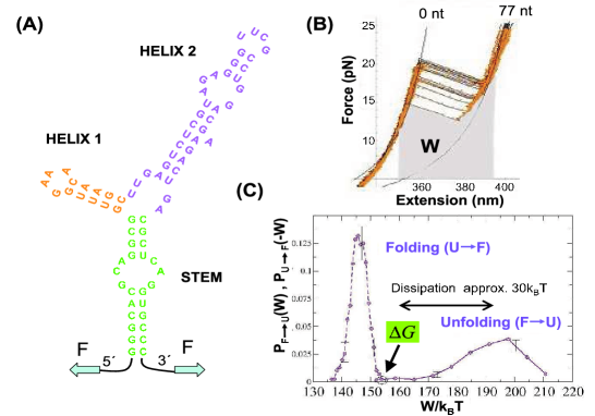
Figure 1: Work statistics in RNA stretching, from R (06)

I.6 Continuous time limit

Similar considerations apply to nonstationary continuous-time  Markov processes.  On the formal level,  such processes may be obtained by taking the limit of discrete-time Markov processes when their time-step $\,\epsilon\,$ tends to zero with the total time interval $\,N\epsilon=\tau\,$ kept constant, provided that the transition probabilities for $\,n\,$ such that $\,n\hskip 0.28436pt\epsilon=t\,$ is fixed have the behavior

$$P_{n}(x,dy)\,=\,\epsilon\hskip 0.28436ptw_{t}(x,dy)\,+\,\Big{(}1-\epsilon\int\limits_{X}w_{t}(x,dz)\Big{)}\,\delta_{x}(dy)\ +\ o(\epsilon)\,.$$ (1.35)

Here $\,\delta_{x}(dy)\,$ denotes the Dirac measure supported at $\{x\}$.  The limiting continuous-time Markov process $\,(x_{t})\,$ for $\,t\in[0,\tau]\,$ has the initial distribution $\,\mu_{0}(dx)$.  Quantities $\,w(x,dy)$,  that are defined modulo signed measures concentrated on the diagonal, may be distributional but are positive measures away from the diagonal and give there the transition rates of the continuous time Markov process. The backward generators of the limiting process defined by the identity

$$\frac{d}{dt}\,\hskip 0.56917pt\mathbb{E}_{\mu_{0}}\,\hskip 0.56917ptf(x_{t})\ =\ \mathbb{E}_{\mu_{0}}\,\hskip 0.56917pt(L_{t}f)(x_{t})$$ (1.36)

are given by the formula

$$(L_{t}f)(x)\,=\,\int\limits_{\cal X}\big{(}f(y)-f(x)\big{)}\,w_{t}(x,dy)\,.$$ (1.37)

The transition probabilities $\,P_{s,t}(x,dy)\,$ of the process $\,(x_{t})\,$ for $\,s\leq t\,$ evolve in time according to the equations

$$\partial_{s}P_{s,t}(x,dy)\,=\,-\,L_{s}(x)\,P_{s,t}(x,dy)\,,\qquad\partial_{t}P_{s,t}(x,dy)\,=\,L^{*}_{t}(y)\,P_{s,t}(x,dy)\,,$$ (1.38)

where $L_{t}^{*}$ is the adjoint operator acting on measures.  At equal times, $\,P_{t,t}(x,dy)=\delta_{x}(dy)$.  In the operator notation,

$$P_{s,t}\,=\,\overrightarrow{\exp}\Big{[}\int\limits_{s}^{t}L_{\sigma}\,d\sigma\Big{]}$$ (1.39)

with the time-ordered exponential, where we write the 1-dimensional Lebesgue measure $\,\lambda(d\sigma)\,$ as $\,d\sigma$.  The time $t$ probability distributions $\,\mu_{t}(dx)\,$ of the process defined by

$$\mathbb{E}_{\mu_{0}}\,f(x_{t})\,=\,\int\limits_{X}f(y)\,\mu_{t}(dy)$$ (1.40)

are given by the relation

$$\mu_{t}(dy)\,=\,\int\limits_{X}\mu_{0}(dx)\,P_{0,t}(x,dy)\,.$$ (1.41)

They evolve according to the equation

$$\partial_{t}\mu_{t}\,=\,L_{t}^{*}\mu_{t}\,.$$ (1.42)

On the other hand,  measures $\nu_{t}(dx)\,$ satisfying the relation

$$L^{*}_{t}\nu_{t}\,=\,0\,.$$ (1.43)

will be said to accompany the process. They would be invariant under time evolution if the transition rates where fixed at the subsequent times to their times-$t$ values.

If state space $\,{\cal X}\,$ is discrete,  a continuous time Markov process jumps from $\,x(t)=x\,$ to $\,x(t+dt)=y\not=x\,$ with probability $\,w(x,dy)dt\,$ and otherwise stays at $x$.  If $\,{\cal X}=\mathbb{R}^{d}$,  the process is a diffusion with a drift or a jump process or a combination of both.

Examples 1.  A general diffusion process.

Consider a stochastic differential equation in $\,\mathbb{R}^{d}\,$

$$dx\,=\,X_{0t}(x)\hskip 0.85355ptdt\,+\,X_{\alpha t}(x)\circ dW_{\alpha}(t)\,,$$ (1.44)

written with the  Stratonovich convention  indicated by symbol $\circ$,  with arbitrary time-dependent vector fields $\,X_{0t},\,X_{\alpha t},\ \alpha=1,\dots,A\,$ and independent standard one-dimensional  Wiener processes $\,W_{\alpha}(t)\,$ (we employ the summation convention so $\alpha$ is summed over).   Eq. (1.44), together with the initial distribution, defines a continuous-time Markov process with transition rates

$$w_{t}(x,dy)\,=\,\big{(}X_{0t}(x)\cdot\nabla_{x}+\frac{{}_{1}}{{}^{2}}(X_{\alpha t}(x)\cdot\nabla_{x})^{2}\big{)}\hskip 0.56917pt\delta(x-y)\,\lambda(dy)$$ (1.45)

and the backward generator

$$L_{t}\,=\,X_{0t}\cdot\nabla\,+\,\frac{{}_{1}}{{}^{2}}\,(X_{\alpha t}\cdot\nabla)^{2}\,.$$ (1.46)

The densities of the time $t$ measures $\,\mu_{t}(dx)=\rho_{t}(x)\,\lambda(dx)\,$ of the process evolve according to the Fokker-Planck equation

$$\partial_{t}\rho_{t}(x)\,=\,L_{t}^{\dagger}\rho_{t}(x)\,=\,-\nabla\cdot j_{t}(x)\,,$$ (1.47)

where $L_{t}^{\dagger}$ is the formal adjoint of $L_{t}$ with respect to the Lebesgue measure $\lambda(dx)$ and

$$j_{t}(x)\,=\,\Big{(}\rho_{t}\,X_{0t}\,-\,\frac{{}_{1}}{{}^{2}}\,\big{(}\nabla\cdot(\rho_{t}X_{\alpha t})\big{)}\,X_{\alpha t}\Big{)}(x)\,\,=\,\big{(}\rho_{t}\,\widehat{X}_{0t}\,-\,{\cal D}_{t}\nabla\rho_{t}\big{)}(x)\,\equiv\,j_{\rho_{t}}(x)$$ (1.48)

is the  probability current,  where

$$\widehat{X}_{0t}\,=\,X_{0t}-\frac{{}_{1}}{{}^{2}}(\nabla\cdot X_{\alpha t})X_{\alpha t}\,,\qquad{\cal D}_{t}\,=\,\frac{{}_{1}}{{}^{2}}X_{\alpha t}\otimes X_{\alpha t}\,.$$ (1.49)

If,  following N (67),  we introduce the  current velocity $\,v_{t}(x)\,$ by the relation

$$j_{t}\,=\,\rho_{t}\hskip 0.28436ptv_{t}$$ (1.50)

then the Fokker-Planck equation (1.47) may be rewritten as the advection equation

$$\partial_{t}\rho_{t}\,+\,\nabla\cdot(\rho_{t}v_{t})\,=\,0\,,$$ (1.51)

which will be used a lot below. Note, nevertheless, that

$$v_{t}\,=\,\widehat{X}_{0t}-\,{\cal D}_{t}\nabla\ln{\rho_{t}}$$ (1.52)

depends on $\rho_{t}$.  The current velocity may be interpreted as the mean velocity of the process conditioned to pass at time $\,t\,$ through point $\,x\,$:

$$v_{t}(x)\,=\,\frac{{\mathbb{E}}_{\mu_{0}}\,\delta(x-x_{t})\circ\frac{dx_{t}}{dt}}{\rho_{t}(x)}\,=\,\frac{\lim\limits_{\epsilon\to 0}\,{\mathbb{E}}_{\mu_{0}}\,\delta(x-x_{t})\,\frac{x_{t+\epsilon}-x_{t-\epsilon}}{2\epsilon}}{\rho_{t}(x)}\,.$$ (1.53)

Examples 2.  Langevin process.

A particular diffusion process in $\mathbb{R}^{d}$ is given by the  Langevin equation

$$dx\,=\,{\cal M}\big{(}-(\nabla H_{t})(x)+f_{t}(x)\big{)}\,dt\,+\,(2{\cal D})^{1/2}dW(t)$$ (1.54)

where ${\cal M}$ (the  mobility)  is a matrix with non-negative symmetric part, and ${\cal D}$ (the diffusivity)  is a non-negative matrix. $\,H_{t}(x)\,$ is the time-dependent Hamiltonian, $\,f_{t}(x)\,$ is a non-conservative force and $\,W(t)\,$ the standard $\,d$-dimensional Wiener process. For simplicity, we took matrices $\,{\cal M}\,$ and $\,{\cal D}\,$ as independent of $\,t\,$ and $\,x$.  The Markov process corresponding to Eq. (1.54) has the transition rates

$$w(x,dy)\,=\,\big{(}-{\cal M}(\nabla H_{t})(x)+{\cal M}f_{t}(x)+{\cal D}\nabla_{x}\big{)}\cdot\nabla_{x}\delta(x-y)\,\lambda(dy)$$ (1.55)

and the backward generator

$$L_{t}\,=\,\big{(}-{\cal M}(\nabla H_{t})+{\cal M}f_{t}(x)+{\cal D}\nabla\big{)}\cdot\nabla\,.$$ (1.56)

The probability current takes in this case the form

$$j_{t}(x)\,=\,\big{(}-{\cal M}(\nabla H_{t})(x)+{\cal M}f_{t}(x)-{\cal D}\nabla\big{)}\hskip 0.56917pt\rho_{t}(x)$$ (1.57)

and the current velocity is

$$v_{t}(x)\,=\,-{\cal M}(\nabla H_{t})(x)+{\cal M}f_{t}(x)-{\cal D}\nabla\ln\rho_{t}(x)\,.$$ (1.58)

One says that ${\cal M}$ and ${\cal D}$ satisfy the  Einstein relation  if

$${\cal M}+{\cal M}^{t}\,=\,2\beta\,{\cal D}\,.$$ (1.59)

If this is the case and the non-conservative force $f_{t}$ vanishes then the Gibbs measures

$$\nu_{t}(dx)\,=\,Z_{t}^{-1}\,{\rm e}^{-\beta H_{t}(x)}\,\lambda(dx)$$ (1.60)

accompany the Markov process described by Eq. (1.54).

Examples 3.  (Einstein-Smoluchowski) Brownian motion.

In the even dimensional case set $x=(q,p)$, where $q$ is the position and $p$ the momentum. Let

$${\cal M}\,=\,\Big{(}\begin{matrix}0&\ -I\cr I&\ M^{-1}\end{matrix}\Big{)}\,,\hskip 77.67589pt{\cal D}\,=\,\Big{(}\begin{matrix}0&\ 0\cr 0&\ M^{-2}D\end{matrix}\Big{)}\,,$$ (1.61)

$$H_{t}(q,p)\,=\,\frac{{}_{1}}{{}^{2}}p\cdot m^{-1}p+U_{t}(x)\,,\qquad\ \,f_{t}(q,p)=(\phi_{t}(x),0)\,,$$ (1.62)

where $M,D,m$ are half-dimension positive matrices, the first two commuting. Then the Langevin stochastic equation takes the form

$$dq\,=\,m^{-1}p\,dt\,,\qquad dp\,=\,\Big{(}-M^{-1}m^{-1}p\,-\,(\nabla U)(q)\,+\,\phi_{t}(q)\Big{)}\,dt\,+\,M^{-1}(2D)^{1/2}\,dW(t)\,.\quad$$ (1.63)

This is the  underdamped  Langevin equation with the Hamiltonian dynamics modified by the addition of friction and random forces.  In this example, one uses the involution $\,(q,p)^{*}=(q,-p)\,$ for the time reversal.  The Einstein relation reads here

$$M\,=\,\beta\hskip 0.56917ptD$$ (1.64)

aligning the inverse friction coefficient $\,M\,$ with the diffusivity $\,D\,$ (physically, both friction and diffusion come from the same source: the interaction with molecules of the thermal environment). The case with $\,U_{t}=0\,$ and $\,\phi_{t}=0\,$ describes the Einstein-Smoluchowski Brownian motion.  In the limit $\,m\to 0$,  the underdamped Langevin equation reduces to the  overdamped  one for $\,q(t)\,$ which reads:

$$dq\,=\,M(-\nabla U_{t}(q)+\phi_{t})\,dt\,+\,(2D)^{1/2}dW(t)\,.$$ (1.65)

This has again the form of Eq. (1.54) with $\,x=q=x^{*}$, $\,{\cal M}=M={\cal M}^{t}\,$ and $\,{\cal D}=D$.

Examples 4.  Lévy process.

The (possibly nonstationary)  Lévy jump process  in $\,\mathbb{R}^{d}\,$ corresponds to the transition probability rates

$$w_{t}(x,dy)\,=\,w_{t}(d(y-x))$$ (1.66)

where $w_{t}(dy)$ is a positive measure.

For a continuous-time Markov process on time interval $\,[0,\tau]$,  the time-reversed process defined by analogy to the one for the discrete-time case has the transition rates

$$w^{\prime}_{t}(x,dy)\,=\,\frac{w_{t^{*}}(y^{*},dx^{*})}{\nu_{t^{*}}(dx^{*})}\,\nu_{t^{*}}(dy^{*})\,,$$ (1.67)

where $\,t^{*}\equiv\tau-t\,$ and an initial measure $\,\mu_{0}^{\prime}$.  By a formal limiting argument, we may infer that the fluctuation relations for the functional $\,{\cal W}[\bm{x}]\,$ defined by relation (1.8) carry over to the case of continuous-time Markov processes. In particular, writing

$$\mu_{0}(dx)\,=\,\rho_{0}(x)\,\lambda(dx)\,,\hskip 25.03856pt\mu_{0}^{\prime}(dx)\,=\,\rho^{\prime}_{0}(x)\,\lambda(dx^{*})\,,$$ (1.68)

(1.69)

$$\nu_{t}(dx)\,=\,{\rm e}^{-\varphi_{t}(x)}\,\lambda(dx)\,,\qquad\nu^{\prime}_{t}(dx)\,=\,{\rm e}^{-\varphi_{t}^{\prime}(x)}\,\lambda(dx^{*})$$ (1.70)

for $\,\varphi^{\prime}_{t}(x)=\varphi_{t^{*}}(x^{*})\,$ and

$${\cal W}[\bm{x}]\,=\,-\,\ln{\rho^{\prime}_{0}(x_{\tau}^{*})}-\varphi_{\tau}(x_{\tau})\,+\int\limits_{0}^{\tau}\partial_{t}\varphi_{t}(x(t))\,dt\,+\,\ln{\rho_{0}(x_{0})}+\varphi_{0}(x_{0})\,=\,-{\cal W}^{\prime}[\bm{x}^{*}]\,,$$ (1.71)

where $\,(\bm{x}^{*})_{t}=x_{t^{*}}^{*}\,$ for $\,\bm{x}=(x_{t})$,  identity (1.8) still holds resulting in relations (1.10) and (1.11).  In the special case when $\,\mu_{0}=\nu_{0}\,$ and $\,\mu^{\prime}_{0}=\nu^{\prime}_{0}$,  expression (1.71) reduces to

$${\cal W}[\bm{x}]\,=\,\int\limits_{0}^{\tau}(\partial_{t}\varphi_{t})(x_{t})\,dt$$ (1.72)

and we obtain the Hatano-Sasa equality HS (01)

$$\boxed{\,\mathbb{E}_{\nu_{0}}\ {\rm e}^{-\int\limits_{0}^{\tau}(\partial_{t}\varphi_{t})(x_{t})\,dt}\,=\,1\,}\,,$$ (1.73)

see Eq. (1.19),  and, if the direct and the reversed process have the same law, also the identity (1.20).

The detailed balance condition for the continuous-time Markov process is defined similarly as for the discrete time and takes the form

$$\lambda(dx)\,w_{t}(x,dy)\,=\,\lambda(dy)\,w_{t}(y,dx)\,{\rm e}^{-\beta(H_{t}(y)-H_{t}(x))}\,,$$ (1.74)

compare to Eq. (1.21). It implies again that the Gibbs measures

$$\nu_{t}(dx)\,=\,Z_{t}^{-1}\,{\rm e}^{-\beta H_{t}(x)}\,\lambda(dx)\,.$$ (1.75)

accompany the process. The transition rates for the time-reversed process take then the form

$$w^{\prime}_{t}(x,dy)\,=\,w_{t^{*}}(x^{*},dy^{*})$$ (1.76)

and one obtains (the continuum time versions of) the Jarzynski equality (1.25) and of the Crooks identity (1.34) for

$$W[\bm{x}]\,=\,\int\limits_{0}^{\tau}(\partial_{t}H_{t})(x_{t})\,dt$$ (1.77)

and $\,W^{\prime}(\bm{x})\,$ given by the similar formula with $\,H_{t}(x)\,$ replaced by $\,H^{\prime}_{t}(x)=H_{t^{*}}(x^{*})$.  Inequality (1.27) also carries over to the continuous time case.

I.7 Fluctuation relations for general diffusion processes

The examples of fluctuation relations discussed above constitute a tip on an iceberg of more general relations of similar type. In particular, in CG (08), we established a family of fluctuation relations for general diffusion processes solving stochastic equations (1.44) on the time interval $\,[0,\tau]$.  Upon an arbitrary division of the drift field

$$X_{0t}(x)\,=\,X^{+}_{0t}(x)+X^{-}_{0t}(x)\,,$$ (1.78)

we defined the time-reversed diffusion process as the one corresponding to the drift and diffusion vector fields

$$X^{\prime}_{0t}\,=\,(X^{+}_{0\hskip 0.28436ptt^{*}})^{*}-(X^{-}_{0\hskip 0.28436ptt^{*}})^{*}\,,\qquad X^{\prime}_{\alpha t}\,=\,(X_{\alpha\hskip 0.28436ptt^{*}})^{*}\,,$$ (1.79)

where $\,X^{*}$ is the push forward of the vector field $\,X\,$ by an involution $\,x\mapsto x^{*}$,  i.e.

$$(X^{*})^{i}(x^{*})\,=\,\frac{\partial{x^{*}}^{i}}{\partial x^{j}}\,X^{j}(x)$$ (1.80)

in coordinates. In other words, $\,X^{+}_{0}\,$ was chosen to transform by the vector and $\,X^{-}_{0}\,$ by the pseudo-vector rule under the involution $\,x\mapsto x^{*}$.  The choice of the rule for $\,X_{\alpha}\,$ is immaterial. We showed, combining the Girsanov and Feynman-Kac formulas, that in this case the functionals $\,{\cal W}[\bm{x}]\,$ and ${\cal W}^{\prime}[\bm{x}]\,$ defined by relation (1.8) have the form

$${\cal W}[\bm{x}]\,=\,-\,\ln\rho_{0}^{\prime}(x_{\tau}^{*})\,+\,\int\limits_{0}^{\tau}{\cal J}_{t}[\bm{x}]\,dt\,+\,\ln\rho_{0}(x_{0})\,=\,-{\cal W}^{\prime}[\bm{x}^{*}]\,,$$ (1.81)

where

$${\cal J}_{t}[\bm{x}]\,=\,\widehat{X}^{+}_{0t}(x_{t})\cdot{\cal D}_{t}^{-1}(x_{t})\Big{(}\circ\frac{dx_{t}}{dt}-X^{-}_{0t}(x_{t})\Big{)}\,-\,\nabla\cdot X^{-}_{0t}(x_{t})$$ (1.82)

in the notations of (1.49).  For the sake of illustration, let us consider four particular time reversals.

I.7.1 Case (a)

First, we shall show that the case studied before is, indeed, a particular instance of such a general scheme. Upon taking

$$\widehat{X}^{+}_{0t}(x)\,=\,-\,{\cal D}_{t}(x)\,\nabla\varphi_{t}(x)$$ (1.83)

for $\,{\rm e}^{-\varphi_{t}}\,$ such that $\,L_{t}^{\dagger}{\rm e}^{-\varphi_{t}}=0$,  we obtain

$${\cal J}_{t}[\bm{x}]\,=\,-\,\nabla\varphi_{t}(x_{t})\cdot\Big{(}\circ\frac{dx_{t}}{dt}-X^{-}_{0t}(x_{t})\Big{)}\,-\,\nabla\cdot X^{-}_{0t}(x_{t})\,=\,-\,\nabla\varphi_{t}(x_{t})\cdot\circ\frac{dx_{t}}{dt}\,.$$ (1.84)

The last equality holds because, with the use of (1.49),

$$0\ =\ {\rm e}^{\varphi_{t}}\hskip 0.85355ptL_{t}^{\dagger}{\rm e}^{-\varphi_{t}}\,=\,{\rm e}^{\varphi_{t}}\hskip 0.85355pt\partial_{i}\Big{(}-X_{0t}^{i}\hskip 0.85355pt{\rm e}^{-\varphi_{t}}\,+\,\frac{{}_{1}}{{}^{2}}\,X_{\alpha t}^{i}\hskip 0.56917pt\partial_{j}\big{(}X_{\alpha t}^{j}{\rm e}^{-\varphi_{t}}\big{)}\Big{)}$$ (1.85)

$$=\,{\rm e}^{\varphi_{t}}\hskip 0.85355pt\nabla\cdot\Big{(}-\widehat{X}_{0t}\hskip 0.85355pt{\rm e}^{-\varphi_{t}}\,+\,\widehat{X}_{0t}^{+}\hskip 0.56917pt{\rm e}^{-\varphi_{t}}\Big{)}\,=\,-\,{\rm e}^{\varphi_{t}}\hskip 0.85355pt\nabla\cdot\Big{(}X_{0t}^{-}\hskip 0.85355pt{\rm e}^{-\varphi_{t}}\Big{)}\,=\,(\nabla\varphi_{t})\cdot X^{-}_{0t}\,-\,\nabla\cdot X^{-}_{0t}\,.\qquad$$ (1.86)

Now,  since

$$-\int\limits_{0}^{\tau}\nabla\varphi_{t}(x_{t})\cdot\circ\hskip 0.56917ptdx_{t}\,=\,-\varphi_{\tau}(x_{\tau})+\varphi_{0}(x_{0})\,+\int\limits_{0}^{\tau}(\partial_{t}\varphi_{t})(x_{t})\,dt\,,$$ (1.87)

functional (1.81) reduces in this case to expression (1.71).

I.7.2 Case (b)

In another important example that will be used below, let us take $\,X_{0t}=X_{0}+Y_{t}\,$ with $\,X_{0}\,$ and $\,X_{\alpha}\,$ time independent.  Let $\,d\nu(dx)={\rm e}^{-\varphi(x)}\lambda(dx)\,$ be the invariant measure for $Y_{t}=0$.  Taking

$$\widehat{X}^{+}_{0t}\,=\,-\,{\cal D}(x)\,\nabla\varphi(x)$$ (1.88)

and proceeding as before, we obtain

$${\cal J}_{t}[\bm{x}]\,=\,-\nabla\varphi(x_{t})\cdot\Big{(}\circ\frac{dx_{t}}{dt}-Y_{t}(x_{t})\Big{)}\,-\,\nabla\cdot Y_{t}(x_{t})\,.$$ (1.89)

I.7.3 Case (c)

Taking $\,X^{+}_{0t}=X_{0t}\,$ so that $\,X^{-}_{0t}=0\,$ corresponds to

$${\cal J}_{t}[\bm{x}]\,=\,\widehat{X}_{0t}(x_{t})\cdot{\cal D}_{t}^{-1}(x_{t})\circ\frac{dx_{t}}{dt}\,.$$ (1.90)

Such time reversal is usually called the reversed protocol.

I.7.4 Case (d)

Finally, suppose that we split the drift vector field taking

$$\widehat{X}^{+}_{0t}(x)\,=\,0\,.$$ (1.91)

In this case,

$${\cal J}_{t}[\bm{x}]\,=\,-\,\nabla\cdot X^{-}_{0t}(x_{t})\,.$$ (1.92)

The latter time reversal makes sense also in the limit of deterministic dynamical processes with $\,X_{\alpha t}=0\,$ when $\,X_{0t}^{-}=X_{0t}\,$ so that $\,{\cal J}_{t}[\bm{x}]\,$ becomes the phase-space contraction rate. It gives rise in that case to the Evans-Searles transient fluctuation relation ES (94, 02).

Example 5.  Consider the underdamped Langevin dynamics of an  anharmonic chain,  with phase-space points $\,x=(q_{0},p_{0},\dots,q_{L},p_{L})$, $\,q_{i},p_{i}\in\mathbb{R}^{d}$,  which is governed by the stochastic equations

$$dq_{i}\,=\,m^{-1}p_{i}\,dt\,,\qquad dp_{i}\,=\,\Big{(}-M_{i}^{-1}m^{-1}p_{i}-\nabla_{q_{i}}U(\underline{q})\Big{)}+(2\beta_{i}^{-1}M_{i}^{-1})^{1/2}dW_{i}(t)$$ (1.93)

with scalars $\,m,M_{i},\beta_{i}>0\,$ and with potential

$$U(\underline{q})\,=\,\frac{k}{2}\sum\limits_{i=1}^{L}(q_{i}-q_{i-1})^{2}\,+\,\sum\limits_{i=0}^{L}\big{(}\frac{r}{2}q_{i}^{2}+\frac{g}{4}(q_{i}^{2})^{2}\big{)}$$ (1.94)

for $k,r,\hskip 0.56917ptg>0$.  The backward generator of the corresponding Markov process is

$$L\,=\,\sum\limits_{i=0}^{L}\Big{(}m^{-1}p_{i}\cdot\nabla_{{q}_{i}}\,-\,(\nabla_{{q}_{i}}U)(\underline{q})\cdot\nabla_{{p}_{i}}\,-\,M_{i}^{-1}m^{-1}p_{i}\cdot\nabla_{{p}_{i}}\,+\,\beta^{-1}_{i}M_{i}^{-1}\nabla_{{p}_{i}}^{2}\Big{)}.$$ (1.95)

If $\,\beta_{i}\equiv\beta\,$ then the dynamics (1.93) has the Gibbs state $\,\nu(dx)=Z^{-1}\,{\rm e}^{-\beta H(x)}\lambda(dx)\,$ as an invariant measure,  where

$$H(x)\,=\,\sum\limits_{i=0}^{L}\frac{p_{i}^{2}}{2m}\,+\,U(\underline{q})$$ (1.96)

is the Hamiltonian of the chain. We shall be mostly interested in the case when the dynamics inside the chain is Hamiltonian, that is when $\,M_{i}^{-1}=0\,$ for $\,i\not=0,L$.  In that situation, the coefficients $\,\beta_{i}\,$ for $\,i\not=0,L\,$ disappear from the stochastic equations (1.93).  Dividing the drift $\,X_{0}\,$ into the vector and pseudo-vector parts so that

$$X_{0}^{+}(x)\,=\,\big{(}0,-M_{i}^{-1}m^{-1}p_{i}\big{)}\,,\qquad X_{0}^{-}(x)\,=\,\big{(}m^{-1}p_{i},-\nabla_{q_{i}}U(\underline{q})\big{)}$$ (1.97)

one infers from Eq. (1.82) that

$${\cal J}_{t}[\bm{x}]\,=\,-\sum\limits_{i=0}^{L}\beta_{i}\hskip 0.28436ptm^{-1}p_{it}\cdot\big{(}\circ\frac{dp_{it}}{dt}+\nabla_{q_{i}}U(\underline{q}_{t})\big{)}$$ (1.98)

for such a choice. Note that the friction coefficients $\,M_{i}^{-1}\,$ do not enter into the latter expression which also does not depend on the choice of interpolating $\,\beta_{i}$, $\,i\not=0,L$,  if $\,M_{i}^{-1}=0\,$ for $\,i\not=0,L$.  A simple calculation shows that

$${\cal J}_{t}[\bm{x}]\,=\,\frac{d}{dt}\hskip 0.85355pt\ln\rho_{0}(x_{t})\,+\,\sum\limits_{i=1}^{L}(\beta_{i}-\beta_{i-1})\,j_{(i-1,i)}(x_{t})\,,$$ (1.99)

where

$$\mu_{0}(dx) = \rho_{0}(x)\,\lambda(dx)$$ (1.100)

$$= Z_{0}^{-1}\exp\Big{[}\sum\limits_{i=0}^{L}\beta_{i}\big{(}\frac{p_{i}^{2}}{2m}+\frac{r}{2}q_{i}^{2}+\frac{g}{4N}(q_{i}^{2})^{2}\big{)}\,+\,\sum\limits_{i=1}^{L}\frac{\beta_{i-1}+\beta_{i}}{2}\frac{k}{2}(q_{i-1}-q_{i})^{2}\Big{]}\lambda(dx)\quad$$ (1.101)

is the a  local equilibrium  measure and

$$j_{(i-1,i)}(x)\,=\,\frac{k}{{2m}}(p_{i-1}+p_{i})\cdot(q_{i-1}-q_{i})$$ (1.102)

is the  energy  (or  heat)  flux  from site $i-1$ to site $i$.  Taking $\,\mu_{0}^{\prime}=\mu_{0}$,  we obtain from (1.81) the quantity

$${\cal W}[\bm{x}]\,=\,\sum\limits_{i=1}^{L}(\beta_{i}-\beta_{i-1})\int\limits_{0}^{\tau}j_{(i-i,i)}(x_{t})\,dt$$ (1.103)

for which the transient fluctuation relations (1.10) and (1.11) hold with all the implications, e.g. the inequality

$$\mathbb{E}_{\mu_{0}}\,{\cal W}[\bm{x}]\,\geq\,0\,.$$ (1.104)

If the dynamics inside the chain is Hamiltonian then different choices of $\,\beta_{i}\,$ for $\,i\not=0,L\,$ lead to different fluctuation relations for the same system. E.g. for a linear interpolation between $\,\beta_{0}\,$ and $\,\beta_{L}$,

$${\cal W}[\bm{x}]\,=\,(\beta_{L}-\beta_{0})\,\frac{1}{L}\sum\limits_{i=1}^{L}\int\limits_{0}^{\tau}j_{(i-i,i)}(x_{t})\,dt\,,$$ (1.105)

whereas for the piecewise constant interpolation with a jump between sites $i-1$ and $i$,

$${\cal W}[\bm{x}]\,=\,(\beta_{L}-\beta_{0})\,\int\limits_{0}^{\tau}j_{(i-i,i)}(x_{t})\,dt\,.$$ (1.106)

Different choices correspond to different local equilibrium measures $\,\mu_{0}(dx)\,$ none of which is a stationary state if $\,\beta_{0}\not=\beta_{L}\,$ because

$$L^{\dagger}\rho_{0}\,=\,\sum\limits_{i=1}^{L}(\beta_{i}-\beta_{i-1})j_{(i-1,i)}\,\not\equiv 0\,.$$ (1.107)

It was shown in refs. EPR99a ; EPR99b that in the stationary state with an invariant measure $\,\nu(dx)\,$ (that in fact has not been proven to exist for the version of the model that we consider, see however EPR99a ),

$$\mathbb{E}_{\nu}\,{\cal W}[\bm{x}]\,\geq\,0$$ (1.108)

with the equality (for $\,\tau>0\,$) if and only if $\,\beta_{0}=\beta_{N}$.  The expectation on the right hand side of inequality (1.108), unlike the one in (1.104), is independent on the choice of interpolating $\,\beta_{i}\,$ (why?). Taking $\,{\cal W}[\bm{x}]\,$ in the form (1.106), the latter result shows that, in the (putative) stationary state, the heat flows in average from the hot to the cold end of the chain, a reassuring result.

II Stochastic Thermodynamics

Although of tautological origin, the fluctuation relations considered in the previous section have important consequences that permit to make contact with the thermodynamical concepts in simple nonequilibrium situations relevant for the modelisation of dynamics of mesoscopic systems, like colloids, polymers, or bio-molecules, in contact with heat bath(s). Such considerations make up an actively developing field known under the name of Stochastic Thermodynamics, see S (12) for a recent review.

II.1 Entropy and entropy production

Let us return to systems described by discrete-time Markov processes $\,(x_{n})_{n=0}^{N+1}$.  Assuming that the time-$n\,$ distributions $\,\mu_{n}(dx)\,$ of such a Markov process have the form $\,\rho_{n}(x)\,\lambda(dx)\,$ with positive densities relative to the reference measure $\,\lambda(dx)$,  we shall define the time-$n\,$ fluctuating entropy of the system by the Boltzmann-type expression

$$S^{sys}_{n}[\bm{x}]\,=\,-k_{B}\,\ln{\rho_{n}(x_{n})}\,.$$ (2.1)

Note that its expectation value

$${\mathbb{E}}_{\mu_{0}}\,S^{sys}_{n}[\bm{x}]\,=\,-\,k_{B}\int\ln{\rho_{n}(x)}\,\rho_{n}(x)\,\lambda(dx)\,\equiv\,S[\mu_{n}]$$ (2.2)

is the Gibbs-Shannon entropy of measure $\,\mu_{n}$.  The change of the fluctuating entropy of the system during the process is consequently given by the expression

$$\Delta S^{sys}[\bm{x}]\,\equiv\,S^{sys}_{N+1}[\bm{x}]\,-\,S^{sys}_{0}[\bm{x}]\,=\,-\,k_{B}\,\ln{\rho_{N+1}(x_{N+1})}\,+\,k_{B}\,\ln{\rho_{0}(x_{0})}\,.$$ (2.3)

whose average is

$${\mathbb{E}}_{\mu_{0}}\,\Delta S^{sys}[\bm{x}]\ =\ S[\mu_{N+1}]-S[\mu_{0}]\,\equiv\,\Delta S[\mu]\,.$$ (2.4)

Similarly, for a continuous time Markov process $\,(x_{t})_{0\leq t\leq\tau}\,$ with time-$t$ distributions $\,\mu_{t}(dx)=\rho_{t}(x)\,\lambda(dx)$,  we define the fluctuating entropy of the system as

$$S^{sys}_{t}[\bm{x}]\,=\,-\,k_{B}\,\ln{\rho_{t}(x_{t})}\,$$ (2.5)

with the change during the process

$$\Delta S^{sys}[\bm{x}]\,\equiv\,S^{sys}_{\tau}[\bm{x}]\,-\,S^{sys}_{0}[\bm{x}]\,=\,-\,k_{B}\,\ln{\rho_{\tau}(x_{\tau})}\,+\,k_{B}\,\ln{\rho_{0}(x_{0})}$$ (2.6)

and the averages

$${\mathbb{E}}_{\mu_{0}}\,S^{sys}_{t}[\bm{x}]\,=\,S[\mu]\,,\qquad{\mathbb{E}}_{\mu_{0}}\,\Delta S^{sys}[\bm{x}]\,=\,S[\mu_{\tau}]-S[\mu_{0}]\,\equiv\,\Delta S[\mu]\,.$$ (2.7)

Nonequilibrium processes change entropy of both the system and the environment. The total entropy production in the units of the Boltzmann constant $\,k_{B}\,$ will be identified with the functional $\,{\cal W}[\bm{x}]\,$ defined by Eq. (1.8) that compares the path measures of the direct and the time-reversed processes,

$$\Delta S^{tot}[\bm{x}]\,=\,k_{B}\,{\cal W}[\bm{x}]\,,$$ (2.8)

provided that the initial distribution of the time-reversed process is fixed by the final distribution of the direct process by the relations

$$\mu^{\prime}_{0}(dx)\,=\,\begin{cases}\mu_{N+1}(dx^{*})\cr\mu_{\tau}(dx^{*})\end{cases}$$ (2.9)

in the discrete- or continuous-time cases, respectively. Note that the total entropy change $\,\Delta S^{tot}\,$ defined this way is a fluctuating quantity depending on the trajectory $\,\bm{x}\,$ of the Markov process. Fluctuation relation (1.10) for $\,\mu^{\prime}_{0}\,$ fixed according to (2.9) may now be rewritten as the identity

$$\boxed{\,{\mathbb{E}}_{\mu_{0}}\ {\rm e}^{-k_{B}^{-1}\Delta S^{tot}[\bm{x}]}\ =\ 1}\,.$$ (2.10)

Similarly, upon the introduction of the same notions for the time-reversed process, Eq. (1.11) may be rewritten as the relation

$$\boxed{\,{\rm e}^{-k_{B}S}\,p^{tot}(S)\,=\,p^{\prime tot}(-S)}\,,$$ (2.11)

where $\,p^{tot}(S)\,$ ($p^{\prime tot}(S)$)  is the probability density function of the total entropy production in the direct (time-reversed) process. Note the similarity of relation (2.10) to the Hatano-Sasa one (1.19). The latter, however, was obtained for a different choice of the initial distributions, namely, for $\,\mu_{0}(dx)=\nu_{0}(dx)\,$ and $\,\mu^{\prime}_{0}(dx)=\nu^{\prime}_{0}(dx)$.

We may separate the total entropy production into two contributions:

$$\Delta S^{tot}[\bm{x}]\,=\,\Delta S^{sys}[\bm{x}]\,+\,\Delta S^{env}[\bm{x}]$$ (2.12)

where $\,\Delta S^{env}[\bm{x}]\,$ is the (fluctuating) entropy production in the environment. For $\,{\cal W}[\bm{x}]\,$ given by Eqs. (1.17) or (1.71), we obtain:

$$\Delta S^{env}[\bm{x}]\,=\,\begin{cases}-k_{B}\,\varphi_{N}(x_{N+1})\,+\,k_{B}\sum\limits_{n=1}^{N}\big{(}\varphi_{n}(x_{n})-\varphi_{n-1}(x_{n})\big{)}\,+\,k_{B}\,\varphi_{0}(x_{0})\,,\cr-k_{B}\,\varphi_{\tau}(x_{\tau})\,+\,k_{B}\int\limits_{0}^{\tau}(\partial_{t}\varphi)_{t}(x_{t})\,dt\,+\,k_{B}\,\varphi_{0}(x_{0})\,,\end{cases}$$ (2.13)

for discrete or continuous time, respectively, whereas for the diffusion processes employing the more general time-reversal schemes discussed in Sec. I.7,

$$\Delta S^{env}[\bm{x}]\,=\,k_{B}\int\limits_{0}^{\tau}{\cal J}_{t}[\bm{x}]\,dt$$ (2.14)

The entropy production in the environment depends in the latter case on the choice of the time-reversal but the fluctuation relations (2.10) and (2.11) hold for all choices.

II.2 $1^{\rm st}$ Law of Stochastic Thermodynamics

In order to motivate the introduction of the above thermodynamical concepts in the general situation, let us consider the special case when the transition probabilities satisfy the detailed balance conditions (1.21) or (1.74) and and the accompanying measures have the Gibbsian form (1.23) or (1.75). The total entropy production given by Eqs. (2.13) may be rewritten in that case in the form

$$\Delta S^{env}[\bm{x}]\,=\,\frac{W[\bm{x}]\,-\,\Delta H[\bm{x}]}{T}$$ (2.15)

where $\,W[\bm{x}]\,$ is the work given by Eqs. (1.26) or (1.77),

$$\Delta H[\bm{x}]\,\,=\,\begin{cases}H_{N}(x_{N+1})\cr H_{\tau}(x_{\tau})\end{cases}\Bigg{\}}\,-\,H_{0}(x_{0})$$ (2.16)

is the change of energy along trajectory $\,\bm{x}$,  and $\,T\,$ is the temperature.  The $\,{\bf 1}^{\rm\bf st}$ Law of Thermodynamics  expressing the conservation of energy asserts that work minus dissipated heat is equal to the change of internal energy of the system. We shall impose it on the level of fluctuating quantities defining heat dissipated along trajectory $\,\bm{x}\,$ as

$$Q[\bm{x}]\,=\,W[\bm{x}]\,-\,\Delta H[\bm{x}]\,.$$ (2.17)

With such a definition, expression for the entropy production in environment (2.15) becomes the Clausius-type relation

$$\Delta S^{env}[\bm{x}]\,=\,\frac{Q[\bm{x}]}{T}$$ (2.18)

for the change of the entropy in isothermal quasi-stationary processes. The use of such a relation is well justified for an environment with a very fast relaxation leading to a Markovian evolution of the system interacting with it.

II.3 $2^{\rm nd}$ Law of Stochastic Thermodynamics

From the fluctuation relation (2.10) it follows by the Jensen inequality that

$$\boxed{\,{\mathbb{E}}_{\mu_{0}}\,\Delta S^{tot}[\bm{x}]\ \geq\ 0\,.}$$ (2.19)

This is the ${\bf 2}^{\rm\bf nd}$ Law of Stochastic Thermodynamics  formulated as the Clausius inequality. In the case with detailed balance, where

$$\Delta S^{tot}[\bm{x}]\,=\,\Delta S^{sys}[\bm{x}]\,+\,\frac{Q[\bm{x}]}{T}\,=\,\Delta S^{sys}[\bm{x}]\,+\,\frac{W[\bm{x}]-\Delta H[\bm{x}]}{T}\,,$$ (2.20)

the Clausius inequality (2.19) may be rewritten as the lower bound on the mean dissipated heat:

$$\boxed{\,{\mathbb{E}}_{\mu_{0}}\,Q[\bm{x}]\ \geq\ -T\hskip 1.9919pt{\mathbb{E}}_{\mu_{0}}\,\Delta S^{sys}[\bm{x}]\,=\,-T\,\Delta S[\mu]}\,,$$ (2.21)

see Eqs. (2.4) and (2.7),  or as the bound

$${\mathbb{E}}_{\mu_{0}}\,W[\bm{x}]\ \geq\ -\,{\mathbb{E}}_{\mu_{0}}\,\big{(}\Delta H[\bm{x}]\,-\,T\Delta S^{sys}[\bm{x}]\big{)}\ =\ \Delta F\,-\,T\,S[\mu_{0}\|\nu_{0}]\,+\,T\begin{cases}S[\mu_{N+1}\|\nu_{N}]\,,\cr S[\mu_{\tau}\|\nu_{\tau}]\,,\end{cases}$$ (2.22)

where for two probability measures $\,\mu(dx)\,$ and $\,\nu(dx)\,$ absolutely continuous with respect to each other, $\,S[\mu\|\nu]\,$ denotes their relative entropy defined by the formula

$$S[\mu\|\nu]\,=\,\int\ln\Big{(}\frac{\mu(dx)}{\nu(dx)}\Big{)}\,\mu(dx)\,.$$ (2.23)

The relative entropy vanishes for $\,\mu=\nu\,$ and is positive in all other cases. Taking as the initial measure of the process $\,\mu_{0}\,$ the accompanying time-zero Gibbs measure $\,\nu_{0}$,  we infer from inequality (2.22) that the $2^{\rm nd}$ Law of Stochastic Thermodynamics (2.19) is in this case stronger than the bound (1.27) established before, a fact not always appreciated in the literature on Stochastic Thermodynamics where the latter bound is often assimilated with the $2^{\rm nd}$ Law.

For the diffusion processes employing the general time-reversal, as discussed in Sec. I.7, the direct calculation CG (08) gives

$${\mathbb{E}}_{\mu_{0}}\,\Delta S^{tot}[\bm{x}]\,=\,k_{B}\int\limits_{0}^{\tau}dt\int\limits_{\cal X}\big{[}\big{(}\widehat{X}^{+}_{0t}-{\cal D}_{t}\nabla\rho_{t}\big{)}(x)\cdot(\rho_{t}{\cal D}_{t})^{-1}\big{(}\widehat{X}^{+}_{0t}-{\cal D}_{t}\nabla\rho_{t}\big{)}\big{]}(x)\,\lambda(dx)\,,$$ (2.24)

where $\,\rho_{t}(x)\,$ denote, as before, the densities of the time-$t\,$ distributions $\,\mu_{t}(dx)\,$ of the process w.r.t. the reference measure $\,\lambda(dx)$, see Sec. II.4 below for the derivation of the above relation in a special case.  The right hand side is an explicitly non-negative expression that for the time reversal (c) of Sec. I.7.3 reduces to the identity

$${\mathbb{E}}_{\mu_{0}}\,\Delta S^{tot}[\bm{x}]\,=\,k_{B}\int\limits_{0}^{\tau}dt\int\limits_{\cal X}\big{[}v_{t}\cdot{\cal D}_{t}^{-1}v_{t}\big{]}(x)\,\rho_{t}(x)\,\lambda(dx)\,,$$ (2.25)

where $\,v_{t}(x)\,$ is the current velocity given by (1.52).

II.4 Work heat and entropy production in overdamped Langevin dynamics

To illustrate further the above discussion, let us consider a system described by an overdamped Langevin equation (1.65) in $\mathbb{R}^{d}$ with positive mobility and diffusivity matrices $M$ and $D$ related by the Einstein relation (1.64). Stochastic equation (1.65), together with the initial distribution $\,\mu_{0}(dq)$,  defines a nonstationary continuous-time Markov process $\,(q_{t})_{0\leq t\leq\tau}\,$ with transition rates

$$w_{t}(q,dq^{\prime})\,=\,\big{(}-M(\nabla U_{t})(q)+D\nabla_{q}\big{)}\cdot\nabla_{q}\hskip 0.28436pt\delta(q-q^{\prime})\,\lambda(dq^{\prime})$$ (2.26)

satisfying the detailed balance relations

$$\lambda(dq)\,w_{t}(q,dq^{\prime})\,=\,\lambda(dq^{\prime})\,w_{t}(q^{\prime},dq)\,\,{\rm e}^{-\beta\big{(}U_{t}(q^{\prime})-U(q)\big{)}}$$ (2.27)

(check it!). Consequently, the Gibbs measures

$$\nu_{t}(dq)\,=\,Z_{t}^{-1}\,{\rm e}^{-\beta\hskip 0.28436ptU_{t}(q)}\lambda(dq)$$ (2.28)

accompany the process, i.e. $\,L_{t}^{*}\nu_{t}=0\,$ for the backward generators

$$L_{t}=\big{(}-M(\nabla U_{t})+D\nabla\big{)}\cdot\nabla\,.$$ (2.29)

On the other hand, the time-$t\,$ probability distributions $\,\mu_{t}(dq)=\rho_{t}(q)\lambda(dq)\,$ evolve according to the advection equation (1.51) with the current velocity

$$v_{t}(q)\,=\,-\,M(\nabla U_{t})(q)-D\nabla\ln\rho_{t}(q)\,.$$ (2.30)

Definitions (1.77) and (2.17) give here the expressions

$$W[\bm{q}]\,=\,\int\limits_{0}^{\tau}(\partial_{t}U_{t})(q_{t})\,dt$$ (2.31)

for the  work  performed on the system during time interval $[0,\tau]\,$ and

$$Q[\bm{q}]\,=\,W[\bm{q}]-\Delta U[\bm{q}]\,=\,-\int\limits_{0}^{\tau}(\nabla U_{t})(q_{t})\circ dq(t)$$ (2.32)

for the  heat  dissipated in the same time interval. The assignment of the names may seem somewhat arbitrary and counter-intuitive (it is the right-hand-side of (2.32) that looks as the work of the gradient force). To understand it better, let us consider an example of a simple system: a bead connected by a spring to the wall whose position $\,y_{t}\,$ may be manipulated externally, see FIG. 2.

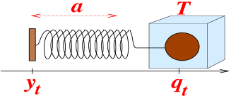
Figure 2: A simple system undergoing an overdamped Langevin dynamics

The position $\,q_{t}\,$ of the bead satisfies the simple overdamped Langevin equation (1.65) with the time-dependent potential $\,U_{t}(q)=\frac{k}{2}(q-a-y_{t})^{2}\,$ if the inertia of the bead can be neglected. In this case,

$$W[\bm{q}]\,=\,-k\int\limits_{0}^{\tau}(q_{t}-a-y_{t})\dot{y}_{t}\hskip 0.85355ptdt$$ (2.33)

is the work performed when externally manipulating the wall and

$$Q[\bm{q}]\,=\,-k\int\limits_{0}^{\tau}(q_{t}-a-y_{t})\circ dq_{t}$$ (2.34)

is the work done on the bead by the force exerted by the spring that, in the overdamped regime, is entirely dissipated as heat due to friction. For more on the rational behind the definition (2.33) of work, see J (07). The mean values of the work and heat are given by the formulae

$${\mathbb{E}}_{\mu_{0}}\,W[\bm{q}] = \int\limits_{0}^{\tau}dt\int(\partial_{t}U)(q)\,\rho_{t}(q)\,\lambda(dq)\,,$$ (2.35)

$${\mathbb{E}}_{\mu_{0}}\,Q[\bm{q}] = {\mathbb{E}}_{\mu_{0}}\,\big{(}W[\bm{q}]-\Delta U[\bm{q}]\big{)}\,=\,\int\limits_{0}^{\tau}dt\bigg{[}\int(\partial_{t}U_{t})(q)\,\rho_{t}(q)\,\lambda(dq)-\frac{d}{dt}\int U_{t}(q)\,\rho_{t}(q)\,\lambda(dq)\bigg{]}$$ (2.36)

$$= -\int\limits_{0}^{\tau}dt\int U_{t}(q)\,\partial_{t}\rho_{t}(q)\,\lambda(dq)\,=\,\int\limits_{0}^{\tau}dt\int U_{t}(q)\,\nabla\cdot(\rho_{t}v_{t})(q)\,\lambda(dq)$$ (2.37)

$$= -\int\limits_{0}^{\tau}dt\int(\nabla U_{t})(q)\cdot(\rho_{t}v_{t})(q)\,\lambda(dq)\,,$$ (2.38)

where we used the advection equation (1.51) assuming that there are no boundary contributions from the integration by parts.

The fluctuating entropy of the system is represented for the overdamped Langevin equation (1.65) by the expression

$$S^{sys}_{t}[\bm{q}]\,=\,-k_{B}\,\ln{\rho_{t}(q_{t})}\,,$$ (2.39)

see (2.5), and the fluctuating total entropy production by

$$\Delta S^{tot}[\bm{q}]\,=\,\Delta S^{sys}[\bm{q}]+\frac{Q[\bm{q}]}{T}\,.$$ (2.40)

For the averages,  this gives:

$${\mathbb{E}}_{\mu_{0}}\,\Delta S^{sys}[\bm{q}]\,=\,\Delta S[\mu]\,=\,-\,k_{B}\int\limits_{0}^{\tau}dt\,\frac{{}_{d}}{{}^{dt}}\int\ln\rho_{t}(q)\,\rho_{t}(q)\,\lambda(dq)$$ (2.41)

$$=k_{B}\int\limits_{0}^{\tau}dt\int\big{[}\nabla\cdot(\rho_{t}v_{t})(q)\,+\,\ln\rho_{t}(q)\,\nabla\cdot(\rho_{t}v_{t})(q)\big{]}\,\lambda(dq)$$ (2.42)

$$=\,-k_{B}\int\limits_{0}^{\tau}dt\int(\nabla\ln\rho_{t})(q)\,(\rho_{t}v_{t})(q)\,\lambda(dq)\,,\qquad\quad$$ (2.43)

and from (2.40), using relation (2.30), we obtain:

$${\mathbb{E}}_{\mu_{0}}\,\Delta S^{tot}[\bm{q}] = k_{B}\int\limits_{0}^{\tau}\big{[}-\beta(\nabla U_{t})-(\nabla\ln{\rho_{t}})\big{]}(q)\cdot(\rho_{t}v_{t})(q)\,\lambda(dq)$$ (2.44)

$$= k_{B}\int\limits_{0}^{\tau}dt\int v_{t}(q)\cdot D^{-1}v_{t}(q)\,\rho_{t}(q)\,\lambda(dq)\,,$$ (2.45)

which is the special case of identity (2.25).

II.5 Landauer Principle

The $2^{\rm nd}$ Law (2.19), rewritten for the non-stationary Markov dynamics satisfying the detailed balance as inequality (2.21), bounds the dissipated heat in terms of the change of the Gibbs-Shannon entropy between initial and final statistical states of the system. In this form, it is closely related to the principle formulated by Landauer in 1961 L (61), see also B (82), stating that the erasure of one bit of information during a computation process conducted in thermal environment requires a release of heat equal to at least $\,k_{B}T\hskip 0.28436pt\ln{2}\,$ (in average). As an example, consider a bi-stable system which may be in two distinct states and which undergoes a process that at final time leaves it always in, say, the second of those states, with a loss of memory of the initial state. Such a device may be realized in the context of Stochastic Thermodynamics by an appropriately designed overdamped Langevin process $\,(q_{t})_{0\leq t\leq\tau}\,$ that starts from the Gibbs state corresponding to a potential $\,R_{0}(q)=-k_{B}T\ln\rho_{0}(q)\,$ with two symmetric wells separated by a high barrier and ends in a Gibbs state corresponding to a potential $\,R_{\tau}(q)=-k_{B}T\ln\rho_{\tau}(q)\,$ with only one of those wells, see FIG. 3.

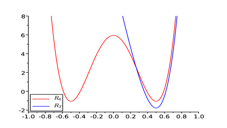
Figure 3: Initial and final Gibbs potentials in a memory erasure process

The change of the Gibbs-Shannon entropy of the system in such a process is approximately

$$\Delta S[\mu]\,\approx\,-\,\ln{1}+\,2\hskip 0.85355pt(\ln{\frac{{}_{1}}{{}^{2}}})\hskip 0.85355pt\frac{{}_{1}}{{}^{2}}\hskip 0.85355pt\,=\,-\hskip 0.85355pt\ln{2}\,,$$ (2.46)

with the better and better approximation the deeper the wells or the lower the temperature. Landauer’s lower bound for average heat release follows now from inequality (2.21) reading

$${\mathbb{E}}_{\mu_{0}}\,Q[\bm{q}]\,\geq\,-T\Delta S[\mu]$$ (2.47)

in the case at hand.

II.6 Finite time Thermodynamics for overdamped Langevin processes

It is well known that the $2^{\rm nd}$ Law bound can be saturated for quasi-stationary processes that move infinitely slowly so that at intermediate times the instantaneous measures $\mu_{t}$ are (almost) equal to the accompanying measures $\nu_{t}$.  Suppose however, that we cannot afford to go too slowly. Indeed, in computational devices, we are interested in fast dynamics that arrives at the final state quickly but produces as little heat as possible. We are therefore naturally led to two questions:

• What is the lower bound for the total entropy production or the average heat release in a process that interpolates between given states in a time interval of fixed duration?

• What is the dynamical protocol that leads to such a minimal total entropy production or heat release?

These questions make sense in a variety of setups. They are among the core ones of the so called Finite-Time Thermodynamics A (11) that was developed during last decades mostly with an eye on technological applications. In the context of Stochastic Thermodynamics, they were first asked and solved for Gaussian overdamped Langevin processes in SS (07). Here we shall study them in the framework of general overdamped Langevin equations (1.65) following AMM (11); AGM (12).

II.7 Benamou-Brenier minimization and optimal mass transport

We would then like to find the minimum of the right hand side of Eq. (2.45) over all control potentials $\,U_{t}\,$ that lead to the overdamped Langevin evolution (1.65) from the fixed initial density $\,\rho_{0}(q)\,$ to the fixed final one $\,\rho_{\tau}(q)\,$ in the fixed time interval $\,[0,\tau]$.  In BB (97, 99),  Benamou-Brenier have solved a closely related problem of minimization of the functional

$$\int\limits_{0}^{\tau}dt\int v_{t}(x)^{2}\,\rho_{t}(x)\,\lambda(dx)$$ (2.48)

over velocity fields $\,v_{t}(q)\,$ constrained by the advection equation (1.51), with the densities $\,\rho_{t}\,$ fixed at the initial and final times. Introducing the positive matrix $\,D^{-1}\,$ into the above functional does not pose a problem (this may be done by a linear change of variables). Note, however, that the current velocities $\,v_{t}\,$ that appear on the right hand side of (2.45) are of the special gradient form, see Eq. (2.30). Let us first ignore the latter restriction at the price that adapting the argument of BB (97, 99) we may end up with a non-optimal bound (this will prove not to be the case a posteriori). Introducing for velocities $\,v_{t}\,$ the Lagrangian flow $\,q_{t}(\bm{x})\,$ satisfying the ODE

$$\partial_{t}q_{t}(q_{0})\,=\,v_{t}(q_{t}(q_{0}))\,,\qquad q_{t}(q_{0})|_{t=0}\,=\,q_{0}\,,$$ (2.49)

and writing the solution of the advection equation in the form

$$\rho_{t}(q)\,=\,\int\delta\big{(}q-q_{t}(q_{0})\big{)}\,\rho_{0}(q_{0})\,\lambda(dq_{0})\,,$$ (2.50)

one may transform the functional on the right hand side of  Eq. (2.45) as follows:

$$\int\limits_{0}^{\tau}dt\int v_{t}(q)\cdot D^{-1}v_{t}(q)\,\rho_{t}(q)\,\lambda(dq) = \int\limits_{0}^{\tau}dt\int\lambda(dq)\int v_{t}(q)\cdot D^{-1}v_{t}(q)\,\,\delta(q-q_{t}(q_{0})\,\lambda(dq_{0})$$ (2.51)

$$= \int\limits_{0}^{\tau}dt\int(\partial_{t}q_{t})(q_{0})\cdot D^{-1}(\partial_{t}q_{t})(q_{0})\,\,\rho_{0}(q_{0})\,\lambda(dq_{0})$$ (2.52)

$$= \int\Big{(}\int\limits_{0}^{\tau}(\partial_{t}q_{t})(q_{0})\cdot D^{-1}(\partial_{t}q_{t})(q_{0})\,dt\Big{)}\,\rho_{0}(q_{0})\,\lambda(dq_{0})\,.\qquad$$ (2.53)

In the first step, one minimizes the right hand side over the curves $\,t\mapsto q_{t}(q_{0})\,$ with fixed endpoint $\,q_{\tau}(q_{0})$. The minima are realized on straight lines leading to the functional

$$\frac{1}{\tau}\int\int(q_{\tau}(q_{0})-q_{0})\cdot D^{-1}(q_{\tau}(q_{0})-q_{0})\,\,\rho_{0}(q_{0})\,\lambda(dq_{0})\ \equiv\ \frac{1}{\tau}\,K[q_{\tau}(\cdot)]$$ (2.54)

that, multiplied by $\,\tau\hskip 0.71114pt$ is, by definition, the quadratic cost function $\,K[q_{\tau}(\cdot)]\,$ of the map $\,q_{0}\mapsto q_{\tau}(q_{0})$.  In the second step, one is left with the celebrated  optimal mass transport  problem of Monge-Kantorovich V (03) consisting of the minimization of quadratic cost $\,K[q_{\tau}(\cdot)]\,$ over the diffeomorphisms $\,q_{0}\mapsto q_{\tau}(q_{0})\,$ under the constraint that

$$\int\limits\int\delta\big{(}q-q_{\tau}(q_{0})\big{)}\,\rho_{0}(q_{0})\,\lambda(dq_{0})\,=\,\rho_{\tau}(q)\,,$$ (2.55)

or,  equivalently, that

$$\rho_{\tau}(q_{\tau}(q_{0}))\,\frac{\partial(q_{\tau}(q_{0}))}{\partial(q_{0})}\,=\,\rho_{0}(q_{0})\,,$$ (2.56)

i.e. demanding that the map $\,q_{0}\mapsto q_{\tau}(q_{0})\,$ transports the density $\,\rho_{0}$ to $\rho_{\tau}$.  One of the results of the optimal mass transport theory states that if the normalized densities $\,\rho_{0}\,$ and $\,\rho_{\tau}\,$ are positive, smooth and have the $2^{\rm nd}$ moments then the minimal cost is attained on a unique diffeomorphism that is a gradient of a smooth convex function

$$q_{\tau}(q_{0})\,=\,D\nabla\hskip 0.71114pt\Psi(q_{0})\,.$$ (2.57)

The corresponding minimizing velocity $\,v_{t}\,$ with the linear Lagrangian flow $\,q^{lin}_{t}(q_{0})\,=\,tq_{0}+(1-t)q_{\tau}(q_{0})\,$ satisfies the  inviscid Burgers equation

$$\partial_{t}v\,+\,v_{t}\cdot\nabla v_{t}\,=\,0$$ (2.58)

(which just states that the Lagrangian trajectories have no acceleration). Even more importantly for us, as a consequence of Eq. (2.57), the minimizing velocity $\,v_{t}\,$ is also of a gradient type:

$$v_{t}\,=\,D\nabla\psi_{t}\,=\,0\,,$$ (2.59)

where the function

$$\psi_{t}(q)\,=\,\frac{1}{2t}(q-q_{0})\cdot D^{-1}(q-q_{0})-\frac{1}{2\tau}q_{0}\cdot D^{-1}q_{0}+\frac{1}{\tau}\Psi(q_{0})\qquad{\rm for}\qquad q=q^{lin}_{t}(q_{0})$$ (2.60)

satisfies the  Hamilton-Jacobi equation

$$\partial_{t}\psi_{t}\,+\,\frac{{}_{1}}{{}^{2}}(\nabla\psi_{t})\cdot D(\nabla\psi_{t})\,=\,0\,.$$ (2.61)

The corresponding interpolating densities $\,\rho_{t}\,$ are given by Eq. (2.50):

$$\rho_{t}(q)\,=\,\int\delta\big{(}q-q^{lin}_{t}(q_{0})\big{)}\,\rho_{0}(q_{0})\,\lambda(dq_{0})\,.$$ (2.62)

Relation (2.59) means that, although the Benamou-Brenier minimization was over general velocities not necessarily of the gradient type,  the minimizer $\,v_{t}\,$ is a current velocity for the overdamped Langevin process with control potential $\,U_{t}\,$ such that

$$\nabla U_{t}\,=\,-\beta^{-1}\nabla\big{(}\psi_{t}+\ln\rho_{t}(q)\big{)},$$ (2.63)

which fixes $\,U_{t}\,$ up to a time-dependent constant. In particular the Benamou-Brenier minimizer also minimizes the right hand side of Eq. (2.45) over the current velocities of the Langevin processes (1.65).

II.8 Finite-time refinement of the $2^{\rm nd}$ Law and of the Landauer bound

We obtain this way

Theorem  (Finite-time refinement of the $\bf 2^{\bf\rm nd}$ Law).  The mean total entropy production in an overdamped Langevin evolution during time $\tau$ between the states with probability densities $\rho_{0}$ and $\rho_{\tau}$ satisfies the bound

$$\boxed{\,\mathbb{E}_{\mu_{0}}\,\Delta S^{tot}[\bm{q}]\ \geq\ \frac{k_{B}}{\tau}\,K_{min}[\rho_{0},\rho_{\tau}]\,}$$ (2.64)

where $\,K_{min}[\rho_{0},\rho_{\tau}]\,$ is the minimal quadratic cost of transport of density $\rho_{0}$ to $\rho_{\tau}$, see (2.54). The above bound is saturated by the optimal protocol with the control potential satisfying Eq .(2.63), where $\,\psi_{t}\,$ and $\,\rho_{t}\,$ are given by Eqs. (2.60) and (2.50), respectively, in terms of the linear interpolation $\,q^{lin}_{t}(q_{0})\,$ between $q_{0}$ and its image $q_{\tau}(q_{0})$ under the optimal transport map.

The above result has a geometric interpretation. The minimal quadratic cost $\,K_{min}(\rho_{0},\rho_{\tau})\,$ is, by definition, the square of the  Wasserstein distance  between the measures $\mu_{0}$ and $\mu_{\tau}$ that, formally, corresponds to the Riemannian metric on the space of probability densities JKO (98), with the square of the tangent vectors given by

$$\|\partial_{t}\rho\|^{2}_{W}\,=\,\int\big{[}(\partial_{t}\rho)(-\nabla\cdot\rho D\hskip 0.56917pt\nabla)^{-1}(\partial_{t}\rho)\big{]}(q)\,\lambda(dq)\,.$$ (2.65)

The Fokker-Planck equation for the (1.47) corresponds to the gradient flow in metric (2.65) for the functional

$$\beta{\cal F}_{t}[\rho]\,=\,\int\big{[}\beta U_{t}+\ln\rho](q)\,\rho(q)\,\lambda(dq)$$ (2.66)

equal, up to the factor $\,\beta$,  to the free energy $\,{\cal F}_{t}[\rho]$,  and one has

$$\mathbb{E}_{\mu_{0}}\,\Delta S^{tot}[\bm{q}]\,=\,k_{B}\int\limits_{0}^{\tau}\|\partial_{t}\rho_{t}\|^{2}_{W}\,dt\,\geq\,\frac{k_{B}}{\tau}\,d_{W}(\mu_{0},\mu_{\tau})^{2}$$ (2.67)

with the optimal protocol giving the (shortest) geodesic between $\rho_{0}$ and $\rho_{\tau}$.

Corollary.  Under the same assumptions, the mean heat release satisfies the bound

$$\mathbb{E}_{\mu_{0}}\,Q_{\tau}[\bm{q}]\,\geq\,=\,-T\Delta S[\mu]\,+\,\frac{k_{B}}{\tau}\,K_{min}[\rho_{0},\rho_{\tau}]\,,$$ (2.68)

with the inequality saturated by the same optimal protocol.

The latter inequality providing a finite-time refinement of the estimate (2.47), implies also a finite-time refinement of the Landauer bound in the situation where the change of the mean system entropy is given by Eq. (2.46). Such a refinement may be relevant in future computer designs S (11) (the present day computers still dissipate much more heat than the minimum allowed by the thermodynamical considerations). A recent experiment B (12) with a colloidal particle manipulated by laser tweezers measured the heat released in a process of memory erasure interpolating at room temperature between two states with Gibbs potential from FIG. 2, with the results plotted in FIG. 3.

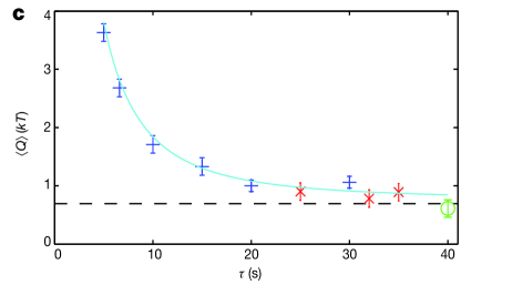
Figure 4: Mean heat release as a function of time in the memory erasure experiment of B (12)

The control potential used in the experiment did not follow the optimal protocol and, as a result, the heat release in the $10s$ run exceeded $2.5$ times the Landauer bound instead of the optimal $40\%$.

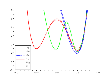
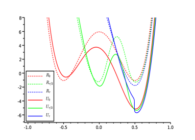
Figure 5: Gibbs and control potentials $R_{t}$ and $U_{t}$ for optimal $10s$ (left) and $1s$ (right) runs

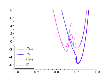
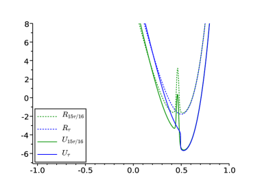
Figure 6: Potentials $R_{t}$ and $U_{t}$ for times $\frac{3}{4}\tau$ and $\tau$ (left) and for $\frac{15}{16}\tau$ and $\,\tau\,$ (right) for $1s$ run

The optimal protocols for $10s$ and $1s$ runs (the latter releasing almost 4 times more heat than the Landauer bound) are illustrated on FIG. 4 at initial, half- and final time. For $10s$, the Gibbs potentials $\,R_{t}=-\beta^{-1}\ln\rho_{t}\,$ are very close to control potentials $\,U_{t}\,$ so that the optimal protocol is almost quasi-stationary. For $1s$, the $\,R_{t}\,$ differ considerable from $\,U_{t}$,  also at the initial and final times, showing a more intricate structure in late times, with the persistence of the barrier separating the two wells, see FIG. 5. The initial and final jumps of the potential in the optimal protocol were first discovered in the case with quadratic potentials by an explicit calculation in SS (07).  The optimal transport map $\,q_{0}\mapsto q_{\tau}(q_{0})\,$ leading to the optimal protocol has the form, in the problem in question, of a kink on the shifted identity map and the corresponding current velocities $v_{t}$ build in time an (almost) shock, see FIG. 6.

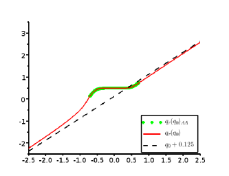
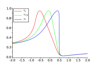
Figure 7: Optimal map $q_{0}\mapsto q_{\tau}(q_{0})$ (left) and the corresponding current velocities (right)

In one dimensional problem as above, the optimal map $\,q_{0}\mapsto q_{\tau}(q_{0})\hskip 1.42271pt$ may be found numerically by sorting the points distributed with densities $\rho_{0}$ and $\rho_{\tau}$ in the increasing order. In more than one dimension, finding such maps requires a more sophisticated Auction Algorithm, see BF (03).

Above, we dealt with nonstationary overdamped Langevin evolution without non-conservative forces. Adding such forces $\,\phi_{t}\,$ as in Eq. (1.65) but keeping the Einstein relation (1.64) modifies the expression (2.32) for the dissipated heat to

$$Q_{\tau}[\bm{q}]\,=\,-\int\limits_{0}^{\tau}\big{(}-\nabla U_{t}+\phi_{t}\big{)}(q_{t})\circ dq(t)\,.$$ (2.69)

The Fokker-Planck equation takes still the form of the advection equation (1.51) but the expression for the current velocity is modified by the addition of $\,\phi_{t}\,$ to

$$v_{t}(q)\,=\,M\big{(}-\nabla U_{t}+\phi_{t}\big{)}(q)-D\nabla\ln\rho_{t}(q)$$ (2.70)

and is no more of the gradient type. The mean total entropy production is still given by Eq. (2.45). Since the Benamou-Brenier minimization held for arbitrary velocities, the bounds (2.64) and (2.68) hold in this case as well, but are saturated by the protocol discussed above without a non-conservative force.

II.9 Generalization to arbitrary diffusions

Much of the discussion of Secs. II.7 and II.8 extends to the general diffusion processes studied in Sec. I.7 with a diffusion matrix $\,{\cal D}_{t}(x)\,$ time-independent and everywhere non-degenerate, provided that we define the total entropy production employing the reversed protocol of Sec. I.7.3. The average total entropy production is then given by expression (2.25) with $\,{\cal D}_{t}(x)={\cal D}(x)$.  The right hand side of Eq. (2.25) may be bounded by the Benamou-Brenier argument of Sec. II.7 resulting in the finite time improvement

$${\mathbb{E}}_{\mu_{0}}\,\Delta^{tot}S[\bm{x}]\ \geq\ \frac{k_{B}}{\tau}K_{min}[\rho_{0},\rho_{\tau}]$$ (2.71)

of the $2^{\rm nd}$ Law.  Now $\,K_{min}[\rho_{0},\rho_{\tau}]\,$ minimizes over the deterministic maps $\,x_{0}\mapsto x_{\tau}(x_{0})\,$ that transport measure $\,\mu_{0}(dx)=\rho_{0}(x)\,\lambda(dx)\,$ to $\,\mu_{\tau}(dx)=\rho_{\tau}(x)\,\lambda(dx)\,$ the quadratic cost $\,K[x_{\tau}(\cdot)]\,$ given by the formula

$$K[x_{\tau}(\cdot)]\,=\,\int\limits_{{\cal X}}d_{{\cal D}^{-1}}(x_{0},x_{\tau}(x_{0}))^{3}\,\rho_{0}(x_{0})\,\lambda(dx_{0})\,,$$ (2.72)

where $\,d_{{\cal D}^{-1}}(x,y)\,$ stands for the distance function in the Riemannian metric $\,g=dx\cdot{\cal D}^{-1}(x)\,dx$.  In-depth information about optimal mass transport in the context of Riemannian geometry may be found in ref. V (04).

More discussion of optimization problems in Stochastic Thermodynamics is contained in refs. GSS (08); EK (10); AMM (12); MMP (12). One of the problems still open is the extension of the above analysis to general underdamped Langevin evolutions which are diffusion processes with degenerate diffusion matrix. For such processes one has to use a different time reversal to define the total entropy production, see Example 5 in Sec. I.7. For general underdamped Langevin processes, the passage in the latter quantity to the overdamped limit contains some surprises, see H (80); SSD (82); CBE (12).

III Fluctuation-dissipation relations

This is a lecture devoted to relations between the fluctuation relations and the laws governing the linear response to perturbations around stationary states that, historically, were among the first results about nonequilibrium dynamics.

III.1 Hatano-Sasa fluctuation relation and the general Fluctuation-Dissipation Theorem

Recall that the Hatano-Sasa transient fluctuation relation (1.73) holds for arbitrary continuous time nonstationary Markov process with backward generators $\,L_{t}\,$ and the family of accompanying measures $\,\nu_{t}(x)={\rm e}^{-\varphi_{t}(x)}\lambda(dx)\,$ such that $\,L_{t}^{*}\nu_{t}=0$.  Following PJP (09), see also H (78), let us consider a family of stationary transition rates $\,w_{\epsilon}(x,dy)\,$ parametrized by $\,\epsilon=(\epsilon^{a})\,$ in a neighborhood of $\,\epsilon=0$,  that correspond to backward generators $\,L_{\epsilon}\,$ with a family of invariant measures $\,\nu_{\epsilon}(dx)\,=\,{\rm e}^{-\varphi_{\epsilon}(x)}\lambda(dx)\,$ such that

$$L_{\epsilon}^{*}\nu_{\epsilon}\,=\,0\,.$$ (3.1)

For each time-dependent protocol $\,t\mapsto\epsilon_{t}\,$ such that $\,\epsilon_{t}=0\,$ for $t\leq 0$, we shall consider for $t\geq 0\,$ the nonstationary Markov process with backward generators $\,L_{\epsilon_{t}}\,$ that starts from the measure $\,\nu\equiv\nu_{0}$.  Note that measures $\,\nu_{\epsilon_{t}}\,$ accompany such a process. For each of protocols $\,\bm{\epsilon}=(\epsilon_{t})$,  we have the Hatano-Sasa relation

$$\mathbb{E}^{\bm{\epsilon}}_{\nu}\,\,{\rm e}^{-\int\limits_{0}^{\tau}\frac{d\epsilon^{a}_{t}}{dt}\,\partial_{\epsilon^{a}}\varphi_{\epsilon_{t}}(x_{t})\,dt}\,=\,1$$ (3.2)

which,  expanded up to the second order in $\bm{\epsilon}$,  gives the identity:

$$-\int\limits_{0}^{\tau}\frac{d\epsilon^{a}_{t}}{dt}\,\mathbb{E}_{\nu}\,\partial_{\epsilon^{a}}\varphi(x_{t})\,dt\,-\,\int\limits_{0}^{\tau}\frac{d\epsilon^{a}_{t}}{dt}\,\epsilon^{b}_{t}\,\mathbb{E}_{\nu}\,\partial_{\epsilon^{b}}\partial_{\epsilon^{a}}\varphi(x_{t})\,dt$$ (3.3)

$$-\,\int\limits_{0}^{\tau}\frac{d\epsilon^{a}_{t}}{dt}\,dt\int\limits_{0}^{\tau}\epsilon^{b}_{s}\,\frac{\delta}{\delta\epsilon_{s}^{b}}\Big{|}_{\bm{\epsilon}=\bm{0}}\,\mathbb{E}_{\nu}^{\bm{\epsilon}}\,\partial_{\epsilon^{a}}\varphi(x_{t})\,\,ds$$ (3.4)

$$+\,\frac{{}_{1}}{{}^{2}}\int\limits_{0}^{\tau}\frac{d\epsilon^{a}_{t}}{dt}\,dt\int\limits_{0}^{\tau}\frac{d\epsilon^{b}_{s}}{dt}\,\mathbb{E}_{\nu}\,\partial_{\epsilon^{b}}\varphi(x_{s})\,\partial_{\epsilon^{a}}\varphi(x_{t})\,\,ds\ =\ 0\,,$$ (3.5)

where $\,\varphi\equiv\varphi_{0}\,$ and $\,\mathbb{E}_{\nu}\equiv\mathbb{E}_{\nu}^{\bm{0}}$.  Expanding similarly the normalization condition

$$\int{\rm e}^{-\varphi_{\epsilon}(x)}\,\lambda(dx)\,=\,1$$ (3.6)

holding for all $\,\epsilon\,$ to the second order, we obtain:

$$\int\Big{(}-\epsilon^{a}\,\partial_{\epsilon^{a}}\varphi(x)\,-\,\frac{{}_{1}}{{}^{2}}\epsilon^{a}\epsilon^{b}\,\partial_{\epsilon^{b}}\partial_{\epsilon^{a}}\varphi(x)\,+\,\frac{{}_{1}}{{}^{2}}\epsilon^{a}\epsilon^{b}\,\partial_{\epsilon^{b}}\varphi(x)\,\partial_{\epsilon^{a}}\varphi(x)\Big{)}\,{\rm e}^{-\varphi(x)}\,\lambda(dx)\,=\,0\,.$$ (3.7)

The last identity implies that

$$\mathbb{E}_{\nu}\,\partial_{\epsilon^{a}}\varphi(x_{t})\,=\,\int\partial_{\epsilon^{a}}\varphi(x_{t})\,\,{\rm e}^{-\varphi(x)}\,\lambda(dx)\,=\,0$$ (3.8)

and that

$$\mathbb{E}_{\nu}\,\partial_{\epsilon^{b}}\partial_{\epsilon^{a}}\varphi(x_{t}) = \int\partial_{\epsilon^{b}}\partial_{\epsilon^{a}}\varphi(x)\,\,{\rm e}^{-\varphi(x)}\,\lambda(dx)\,=\,\int\partial_{\epsilon^{b}}\varphi(x)\,\,\partial_{\epsilon^{a}}\varphi(x)\,\,{\rm e}^{-\varphi(x)}\,\lambda(dx)$$ (3.9)

$$= \mathbb{E}_{\nu}\,\partial_{\epsilon^{b}}\varphi(x_{t})\,\,\partial_{\epsilon^{a}}\varphi(x_{t})\,,$$ (3.10)

where the right hand side is $t$-independent. Substituting these identities to Eq. (3.5), we obtain:

$$-\,\frac{{}_{1}}{{}^{2}}\int\limits_{0}^{\tau}\frac{d\epsilon^{a}_{t}}{dt}\,dt\int\limits_{0}^{\tau}\frac{d\epsilon^{b}_{s}}{ds}\,ds\,\,\mathbb{E}_{\nu}\,\partial_{\epsilon^{b}}\varphi(x_{t})\,\,\partial_{\epsilon^{a}}\varphi(x_{t})\,-\,\int\limits_{0}^{\tau}\frac{d\epsilon^{a}_{t}}{dt}\,dt\int\limits_{0}^{\tau}\epsilon^{b}_{s}\,\frac{\delta}{\delta\epsilon_{s}^{b}}\Big{|}_{\bm{\epsilon}=\bm{0}}\,\mathbb{E}_{\nu}^{\bm{\epsilon}}\,\partial_{\epsilon^{a}}\varphi(x_{t})\,\,ds$$ (3.11)

$$+\,\frac{{}_{1}}{{}^{2}}\int\limits_{0}^{\tau}\frac{d\epsilon^{a}_{t}}{dt}\,dt\int\limits_{0}^{\tau}\frac{d\epsilon^{b}_{s}}{dt}\,\mathbb{E}_{\nu}\,\partial_{\epsilon^{b}}\varphi(x_{s})\,\partial_{\epsilon^{a}}\varphi(x_{t})\,\,ds$$ (3.12)

$$=\ -\,\frac{{}_{1}}{{}^{2}}\int\limits_{0}^{\tau}\frac{d\epsilon^{a}_{t}}{dt}\,dt\int\limits_{0}^{\tau}\frac{d\epsilon^{b}_{s}}{ds}\,\,\mathbb{E}_{\nu}\,\partial_{\epsilon^{a}}\varphi(x_{t})\,\,\partial_{\epsilon^{b}}\varphi(x_{t})\,\,ds$$ (3.13)

$$-\,\int\limits_{0}^{\tau}\frac{d\epsilon^{a}_{t}}{dt}\,dt\int\limits_{0}^{\tau}\frac{d\epsilon^{b}_{s}}{ds}\,ds\int\limits_{s}^{\tau}\frac{\delta}{\delta\epsilon_{\sigma}^{b}}\Big{|}_{\bm{\epsilon}=\bm{0}}\,\mathbb{E}_{\nu}^{\bm{\epsilon}}\,\partial_{\epsilon^{a}}\varphi(x_{t})\,\,d\sigma$$ (3.14)

$$+\,\frac{{}_{1}}{{}^{2}}\int\limits_{0}^{\tau}\frac{d\epsilon^{a}_{t}}{dt}\,dt\int\limits_{0}^{\tau}\frac{d\epsilon^{b}_{s}}{dt}\,\mathbb{E}_{\nu}\,\partial_{\epsilon^{b}}\varphi(x_{s})\,\partial_{\epsilon^{a}}\varphi(x_{t})\,\,ds\ =\ 0\,.$$ (3.15)

Upon stripping of the arbitrary functions $\,\frac{d\epsilon_{t}}{dt}$,  the last equation is equivalent to the identity

$$\mathbb{E}_{\nu}\,\partial_{\epsilon^{b}}\varphi(x_{s})\,\partial_{\epsilon^{a}}\varphi(x_{t})\,-\,\mathbb{E}_{\nu}\,\partial_{\epsilon^{b}}\varphi(x_{t})\,\partial_{\epsilon^{a}}\varphi(x_{t})$$ (3.16)

$$=\,\int\limits_{s}^{\tau}\frac{\delta}{\delta\epsilon_{\sigma}^{b}}\Big{|}_{\bm{\epsilon}=\bm{0}}\,\mathbb{E}_{\nu}^{\bm{\epsilon}}\,\partial_{\epsilon^{a}}\varphi(x_{t})\,d\sigma\,+\,\,\int\limits_{t}^{\tau}\frac{\delta}{\delta\epsilon_{\sigma}^{a}}\Big{|}_{\bm{\epsilon}=\bm{0}}\,\mathbb{E}_{\nu}^{\bm{\epsilon}}\,\partial_{\epsilon^{b}}\varphi(x_{s})\,d\sigma$$ (3.17)

Because, by causality,

$$\frac{\delta}{\delta\epsilon_{\sigma}^{a}}\Big{|}_{\bm{\epsilon}=\bm{0}}\,\mathbb{E}_{\nu}^{\bm{\epsilon}}\,\partial_{\epsilon^{b}}\varphi(x_{s})\,=\,0\qquad{\rm for}\qquad s\leq\sigma\,,$$ (3.18)

Eq. (3.17) reduces upon taking $\,s\leq t\,$ to the relation

$$\mathbb{E}_{\nu}\,\partial_{\epsilon^{b}}\varphi(x_{s})\,\partial_{\epsilon^{a}}\varphi(x_{t})\,-\,\mathbb{E}_{\nu}\,\partial_{\epsilon^{b}}\varphi(x_{t})\,\partial_{\epsilon^{a}}\varphi(x_{t})\,=\,\int\limits_{s}^{t}\frac{\delta}{\delta\epsilon_{\sigma}^{b}}\Big{|}_{\bm{\epsilon}=\bm{0}}\,\mathbb{E}_{\nu}^{\bm{\epsilon}}\,\partial_{\epsilon^{a}}\varphi(x_{t})\,d\sigma\,,\qquad$$ (3.19)

or,  in the differential form,  to the identity

$$\boxed{\,\partial_{s}\,\mathbb{E}_{\nu}\,\partial_{\epsilon^{b}}\varphi(x_{s})\,\partial_{\epsilon^{a}}\varphi(x_{t})\,=\,-\,\frac{\delta}{\delta\epsilon_{s}^{b}}\Big{|}_{\bm{\epsilon}=\bm{0}}\,\mathbb{E}_{\nu}^{\bm{\epsilon}}\,\partial_{\epsilon^{a}}\varphi(x_{t})\,}\,.$$ (3.20)

This a one of general forms of the  Fluctuation-Dissipation Theorem (FDT) H (78); PJP (09). The left hand side is the time derivative of  the  dynamical correlation function  of observables $\,\partial_{\epsilon^{a}}\varphi(x)\,$ in the stationary state, whereas the quantity on the right hand side is the  response function  measuring the change of the dynamical one point function of $\,\partial_{\epsilon^{a}}\varphi(x)\,$ under a small perturbation of $\,\epsilon\,$ concentrated around an earlier time. Note that such a perturbation makes the dynamics nonstationary.  The entry $\,\partial_{\epsilon^{a}}\varphi(x_{t})\,$ plays a passive role in the identity (3.20) and could be replaced by an arbitrary function $\,O_{a}(x_{t})$.  On the other hand, for a general stationary dynamical correlation function with $\,s\leq t\,$ one has

$$\partial_{t}\,\mathbb{E}_{\nu}\,O_{b}(s)\,O_{a}(t)\,=\,\int\nu(dx)\,O_{b}(x)\int\partial_{t}P_{s,t}(x,dy)\,O_{a}(y)\,=\,\mathbb{E}_{\nu}\,O_{b}(s)\,(L\hskip 0.56917ptO_{a})(t)\,,$$ (3.21)

$$\partial_{s}\,\mathbb{E}_{\nu}\,O_{b}(s)\,O_{a}(t)\,=\,\int\nu(dx)\,O_{b}(x)\int\partial_{s}P_{s,t}(x,dy)\,O_{a}(y)\,=\,-\,\mathbb{E}_{\nu}\,(L^{\prime}O_{b})(s)\,(L\hskip 0.56917ptO_{a})(t)\,,\qquad\quad$$ (3.22)

where

$$L^{\prime}\,=\,{\rm e}^{\varphi}\hskip 0.85355ptL^{\dagger}\,{\rm e}^{-\varphi}$$ (3.23)

is the adjoint of $\,L\,$ with respect to the invariant measure $\,\nu(dx)$.  We infer that the FDT (3.20) may be rewritten in the form

$$\,\mathbb{E}_{\nu}\,L^{\prime}\big{(}\partial_{\epsilon^{b}}\varphi(x_{s})\big{)}\,\,O_{a}(x_{t})\,=\,\frac{\delta}{\delta\epsilon_{s}^{b}}\Big{|}_{\bm{\epsilon}=\bm{0}}\,\mathbb{E}_{\nu}^{\bm{\epsilon}}\,O_{a}(x_{t})\,.$$ (3.24)

III.2 Other forms of the Fluctuation-Dissipation Theorem

We shall follow in this section the approach to the FDT developed in CG . Let us consider a particular family of transition rates of the form

$$w_{\epsilon}(x,dy)\,=\,{\rm e}^{-\frac{\beta}{2}\epsilon^{a}O_{a}(x)}\hskip 0.85355ptw(x,dy)\,{\rm e}^{\frac{\beta}{2}\epsilon^{a}(O_{a}(y))}$$ (3.25)

for a family of functions $\,O_{a}(x)$,  corresponding to the perturbed backward generators

$$L_{\epsilon} = {\rm e}^{-\frac{\beta}{2}\epsilon^{a}O_{a}(x)}L\,{\rm e}^{\frac{\beta}{2}\epsilon^{a}O_{a}(x)}\,-\,{\rm e}^{-\frac{\beta}{2}\epsilon^{a}O_{a}(x)}\big{(}L\hskip 0.85355pt{\rm e}^{\frac{\beta}{2}\epsilon^{a}O_{a}(x)}\big{)}$$ (3.26)

$$= L\,+\,\frac{{}_{\beta}}{{}^{2}}\epsilon^{a}\Big{(}[L,O_{a}]-(L\hskip 0.56917ptO_{a})\Big{)}\ +\ o(\epsilon)\,.$$ (3.27)

Above, $\,\beta\,$ is introduced just for dimensional reason, see however below. The invariance condition (3.1) for the measures $\,\nu_{\epsilon}(dx)\,$ gives now to the $1^{\rm st}$ order in $\,\epsilon\,$ the condition

$$-\,\epsilon^{a}\,L^{\dagger}\big{(}{\rm e}^{-\varphi}\,\partial_{\epsilon^{a}}\varphi\big{)}\,+\,\frac{{}_{\beta}}{{}^{2}}\epsilon^{a}\Big{(}[L,O_{a}]-(L\hskip 0.56917ptO_{a})\Big{)}^{\dagger}\big{(}{\rm e}^{-\varphi}\big{)}\,=\,0\,,$$ (3.28)

i.e.

$$L^{\prime}\big{(}\partial_{\epsilon^{a}}\varphi\big{)}\,=\,-\,\frac{{}_{\beta}}{{}^{2}}\big{(}L^{\prime}O_{a}\,+\,L\hskip 0.56917ptO_{a}\big{)}\,.$$ (3.29)

Plugging this expression into Eq. (3.24), we may rewrite it in the form

$$\boxed{\,\partial_{s}\,\mathbb{E}_{\nu}\,O_{b}(x_{s})\,O_{a}(x_{t})\,-\,\mathbb{E}_{\nu}(L\hskip 0.56917ptO_{b})(x_{s})\,O_{a}(x_{t})\,=\,\frac{2}{\beta}\,\frac{\delta}{\delta\epsilon_{s}^{b}}\Big{|}_{\bm{\epsilon}=\bm{0}}\,\mathbb{E}_{\nu}^{\bm{\epsilon}}\,O_{a}(x_{t})\,}\,.$$ (3.30)

This is another form of the general FDT CKP (94); LCZ (05); BMW (09). It does not require the knowledge of the invariant states, but involves explicitly the generator of the stationary process.

We may also rewrite the right hand side of Eq. (3.29) as $\,\,-\,\beta L^{\prime}O_{a}\,-\,\frac{{}_{\beta}}{{}^{2}}(L-L^{\prime})O_{a}$.  This results in yet another form of the general FDT:

$$\partial_{s}\,\mathbb{E}_{\nu}\,O_{b}(x_{s})\,O_{a}(x_{t})\,-\,\mathbb{E}_{\nu}\,\big{(}\frac{{}_{1}}{{}^{2}}(L-L^{\prime})O_{b}\big{)}(x_{s})\,O_{a}(x_{t})\Big{)}\,=\,\frac{1}{\beta}\,\frac{\delta}{\delta\epsilon_{s}^{b}}\Big{|}_{\bm{\epsilon}=\bm{0}}\,\mathbb{E}_{\nu}^{\bm{\epsilon}}\,O_{a}(x_{t})\,.$$ (3.31)

The latter form is useful for the Langevin process where

$$L\,=\,\big{(}-{\cal M}(\nabla H)+{\cal M}f+{\cal D}\nabla\big{)}\cdot\nabla$$ (3.32)

and were

$$L^{\prime} = {\rm e}^{\varphi}\,L^{\dagger}\,{\rm e}^{-\varphi}\,=\,\big{(}{\cal M}(\nabla H)-{\cal M}f\big{)}\cdot\nabla\,+\,2\,{\rm e}^{\varphi}\,(\nabla\cdot{\rm e}^{-\varphi}){\cal D}\nabla\,+\,\nabla\cdot{\cal D}\nabla$$ (3.33)

since $\,L^{\dagger}({\rm e}^{-\varphi})=0$.  Hence in this case,

$$\frac{{}_{1}}{{}^{2}}(L-L^{\prime})\,=\,\big{(}-{\cal M}(\nabla H)+{\cal M}f-{\rm e}^{\varphi}{\cal D}(\nabla{\rm e}^{-\varphi})\big{)}\cdot\nabla\,=\,v\cdot\nabla\,,$$ (3.34)

where $\,v(x)\,$ is the current velocity, see Eq. (1.58), in the stationary state. Using the the latter relation, we obtain the general FDT for the Langevin dynamics CFG (08):

$$\boxed{\,\partial_{s}\,\mathbb{E}_{\nu}\,O_{b}(x_{s})\,O_{a}(x_{t})\,-\,\mathbb{E}_{\nu}\,\big{(}v\cdot\nabla O_{b}\big{)}(x_{s})\,O_{a}(x_{t})\Big{)}\,=\,\frac{1}{\beta}\,\frac{\delta}{\delta\epsilon_{s}^{b}}\Big{|}_{\bm{\epsilon}=\bm{0}}\,\mathbb{E}_{\nu}^{\bm{\epsilon}}\,O_{a}(x_{t})\,}\,.$$ (3.35)

Note that for the stationary Langevin process with $\,{\cal M}={\cal M}^{t}=\beta{\cal D}$, the perturbation (3.25) corresponds to the change of the Hamiltonian $\,H(x)\to H(x)-\epsilon^{a}O_{a}(x)$.

In the situation with detailed balance for the stationary process with $\,\epsilon=0$,  see Eq. (1.74),  generators $\,L\,$ and $\,L^{\prime}\,$ coincide and $\,\varphi_{\epsilon}(x)=\beta\big{(}H(x)\,-\,\epsilon^{a}O_{a}(x)-\,F_{\epsilon}\big{)}$,  where $\,F_{\epsilon}\,$ is a constant. As a result, all three forms of the FDT reduce to the identity

$$\boxed{\,\partial_{s}C^{ab}(t-s)\,\equiv\,\partial_{s}\,\mathbb{E}_{\nu}\,O_{b}(x_{s})\,O_{a}(x_{t})\,=\,\frac{1}{\beta}\,\frac{\delta}{\delta\epsilon_{s}^{b}}\Big{|}_{\bm{\epsilon}=\bm{0}}\,\mathbb{E}_{\nu}^{\bm{\epsilon}}\,O_{a}(x_{t})\,\equiv\,\frac{1}{\beta}\,R^{ab}(t-s)\,}$$ (3.36)

which is the classic equilibrium FDT K (57) relating the equilibrium dynamical correlation function $\,C^{ab}(t-s)\,$ to the response function $\,R^{ab}(t-s)\,$ of the equilibrium state to small perturbations.

Example 6.  For the Einstein-Smoluchowski Brownian motion of Example 3 with scalar mass matrix $\,m$, $\,O_{a}(q,p)=p^{a}\,$ and $\,O_{b}(q,p)=q^{b}$,  the stationary form of the dynamical correlation function is

$$C^{ab}(t-s)\,=\,m\hskip 0.85355ptD\,\delta^{ab}\,{\rm e}^{-\frac{t-s}{mM}}$$ (3.37)

(there is no complete stationary state in that case since the expectation value of $\,q_{t}^{2}\,$ diverges linearly in time),  and the response function takes the form

$$R^{ab}(t-s)\,=\,\delta^{ab}\,{\rm e}^{-\frac{t-s}{mM}}\,.$$ (3.38)

Relation (3.36) reduces then to the Einstein relation (1.64),  a prototype of the equilibrium FDT.

The possible usage of the FDT (3.36) is for extracting the response function, more difficult to measure, from the stationary dynamical correlation function, more easily accessible, or for inferring the temperature $\beta^{-1}$ of a system in thermal equilibrium if both the response function and the dynamical correlation function are accessible. Although near a nonequilibrium stationary states (NESS), the FDT does not have such a simple form, the ratio of the dynamical correlation to the response function is often used for systems out of equilibrium, in particular in glassy systems C (11), to define their effective temperatures.

It was observed in CFG (08)), see also SS (06), that the form (3.35) of the FDT for Langevin systems implies that one recovers the equilibrium form of the FDT in Lagrangian frame of the current velocity. It was shown subsequently in CG (09) that any nonequilibrium Langevin diffusion rewritten in the Lagrangian frame of its current velocity recovers the detailed balance property.

III.3 Relation of the response function to dissipation

The original name of the Fluctuation-Dissipation Theorem for the identity (3.36) comes from the fact that the dynamical 2-time correlation function describes the correlation between the fluctuations of the random variables $\,O(x_{t})$ whereas the response function is related to dissipation of energy or heat. To understand the latter connection, let us consider the case of a periodic perturbation of the stationary equilibrium dynamics by taking $\,\epsilon_{t}=\epsilon_{0}\sin(\omega t)\,$ so that $\,H_{t}(x)\,=\,H(x)-\epsilon_{0}\sin(\omega t)\,O(x)$. For such a system, the average expectation of the work

$$W_{\tau}[\bm{x}]\,=\,\int\limits_{0}^{\tau}(\partial_{t}H_{t})(x_{t})\,dt\,=\,-\,\epsilon_{0}\hskip 0.85355pt\omega\int\limits_{0}^{\tau}\cos(\omega t)\,O(x_{t})\,dt$$ (3.39)

is per unit time equal to

$$\lim\limits_{\tau\to\infty}\ \frac{1}{\tau}\,\mathbb{E}_{\nu}^{\bm{\epsilon}}\,W_{\tau}[\bm{x}]\,=\,-\lim\limits_{\tau\to\infty}\ \frac{\epsilon_{0}\hskip 0.56917pt\omega}{\tau}\int\limits_{0}^{\tau}\,\cos(\omega t)\,\mathbb{E}_{\nu}^{\bm{\epsilon}}\,O(x_{t})\,dt$$ (3.40)

$$= -\lim\limits_{\tau\to\infty}\ \frac{\epsilon_{0}\hskip 0.56917pt\omega}{\tau}\int\limits_{0}^{\tau}\,\cos(\omega t)\,\Big{(}\mathbb{E}_{\nu}^{0}\,O(x_{t})\,+\,\epsilon_{0}\int\limits_{0}^{t}\sin(\omega s)\,\frac{\delta}{\delta\epsilon_{s}}\,\mathbb{E}_{\nu}\,O(x_{t})\,ds\,+\,o(\epsilon_{0})\Big{)}\,dt\,.\qquad$$ (3.41)

The stationary contribution vanishes in the long time limit, so that, denoting

$$\frac{\delta}{\delta\epsilon_{s}}\,\mathbb{E}_{\nu}\,O(x_{t})\,\equiv\,R(t-s)\,,$$ (3.42)

we obtain

$$\lim\limits_{\tau\to\infty}\ \frac{1}{\tau}\,\mathbb{E}_{\nu}^{\bm{\epsilon}}\,W_{\tau}[\bm{x}] = -\lim\limits_{\tau\to\infty}\ \frac{\epsilon_{0}^{2}\omega}{\tau}\int\limits_{0}^{\tau}dt\int\limits_{0}^{t}\,\cos(\omega t)\,\sin(\omega s)\,R(t-s)\,ds\ +\ o(\epsilon_{0}^{2})$$ (3.43)

$$= -\lim\limits_{\tau\to\infty}\ \frac{\epsilon_{0}^{2}\omega}{\tau}\int\limits_{0}^{\tau}\sin(\omega s)\,ds\int\limits_{0}^{\tau-s}\,\cos(\omega(s+\sigma))\,R(\sigma)\,d\sigma\ +\ o(\epsilon_{0}^{2})$$ (3.44)

$$= -\lim\limits_{\tau\to\infty}\ \frac{\epsilon_{0}^{2}\omega}{\tau}\Big{(}\int\limits_{0}^{\tau}\sin(\omega s)\cos(\omega s)\,ds\int\limits_{0}^{\tau-s}\,\cos(\omega\sigma)\,R(\sigma)\,d\sigma$$ (3.46)

$$\hskip 42.67912pt-\,\int\limits_{0}^{\tau}\sin^{2}(\omega s)\,ds\int\limits_{0}^{\tau-s}\,\sin(\omega\sigma)\,R(\sigma)\,d\sigma\Big{)}\ +\ o(\epsilon_{0}^{2})$$

$$= \Big{(}\lim\limits_{\tau\to\infty}\ \frac{\epsilon_{0}^{2}\omega}{\tau}\int\limits_{0}^{\tau}\sin^{2}(\omega s)\,ds\Big{)}\,\int\limits_{0}^{\infty}\sin(\omega\sigma)\,R(\sigma)\,d\sigma\ +\ o(\epsilon_{0}^{2})$$ (3.47)

$$= \frac{\epsilon_{0}^{2}\omega}{2}\,{\rm Im}\hskip 0.85355pt\widehat{R}(\omega)\ +\ o(\epsilon_{0}^{2})\,,$$ (3.48)

assuming the integrable decay of $\,R(\sigma)\,$ when $\,\sigma\to\infty$,  where

$$\widehat{R}(\omega)\,=\,\int\limits_{0}^{\infty}{\rm e}^{i\omega\sigma}\,R(\sigma)\,d\sigma$$ (3.49)

is the Fourier transform of the response function (recall that the latter vanishes for negative arguments). In experiments, often the dissipation rate is directly measured, giving access to the imaginary part of the Fourier-space response function $\,\widehat{R}(\omega)$. The real part of $\,\widehat{R}(\omega)\,$ may then be obtained from the imaginary part by the Kramers-Kronig dispersion relation

$${\rm Re}\hskip 0.85355pt\widehat{R}(\omega)\,=\,\frac{{}_{1}}{\pi}\,{\cal P}\int\frac{{\rm Im}\hskip 0.85355pt\widehat{R}(\omega^{\prime})}{\omega^{\prime}-\omega}\,\lambda(d\omega^{\prime})$$ (3.50)

holding for Fourier transforms of function vanishing at negative times.

III.4 A simple one-dimensional example

Let us consider an overdamped Langevin dynamics of a particle moving on a circle that is described by by the stochastic equation

$$d\theta\,=\,M\big{(}F-\partial_{\theta}U(\theta)\big{)}\hskip 0.56917ptdt\,+\,\sqrt{2D}\,dW(t)\,,$$ (3.51)

where $\,\theta\,$ is the angle modulo $\,2\pi\,$ parametrizing the position of the particle, $\,M\,$ is the mobility and $\,D=\beta^{-1}M\,$ is the diffusivity of the particle.  Periodic function $\,U(\theta)\,$ gives the potential and $\,F\,$ is a constant part of the force (any non-conservative force may be separated into a constant plus a potential part in that situation). Eq. (3.51) models the dynamics of a colloidal particle of radius $1\mu m$ kept on a circular trajectory of radius $4.12\mu m$ by a laser tweezer in an experiment performed at ENS Lyon GPC (09) in which case

$$MU(\theta)\,=\,H_{0}\sin(\theta)\qquad{\rm for}\qquad H_{0}=0.87\,rad\,s^{-1},$$ (3.52)

$$MF\,=\,0.85\,rad\,s^{-1}\,,\hskip 46.94687ptD\,=\,1.26\times 10^{-2}\,rad^{2}\,s^{-1}\,.$$ (3.53)

The diffusion (3.51) has the backward generator

$$L\,=\,M\big{(}F-(\partial_{\theta}U)\big{)}\hskip 0.56917pt\partial_{\theta}+D\hskip 0.56917pt\partial_{\theta}^{2}$$ (3.54)

and a NESS with the invariant measure $\,\nu(\theta)=\rho(\theta)\hskip 0.56917pt\lambda(d\theta)\,$ for

$$\rho(\theta)\,=\,Z^{-1}\,{\rm e}^{\,\beta(F\theta-U(\theta))}\int\limits_{\theta}^{\theta+2\pi}{\rm e}^{-\beta(F\vartheta-U(\vartheta))}\,\lambda(d\vartheta)\ \equiv\ {\rm e}^{-\varphi(\theta)}$$ (3.55)

that corresponds to the constant probability current

$$j\,=\,\Big{(}M(F-(\partial_{\theta}U)(\theta))-D\hskip 0.56917pt\partial_{\theta}\Big{)}\hskip 0.56917pt{\rm e}^{-\varphi(\theta)}\,=\,D\hskip 0.56917ptZ^{-1}\Big{(}1-{\rm e}^{-2\pi\beta F}\Big{)}$$ (3.56)

and to the current velocity

$$v(\theta)\,=\,j\,\rho(\theta)^{-1}\,=\,\frac{D(1-{\rm e}^{-2\pi\beta F})}{{\rm e}^{\,\beta(F\theta-U(\theta))}\int\limits_{\theta}^{\theta+2\pi}{\rm e}^{-\beta(F\vartheta-U(\vartheta))}\,\lambda(d\vartheta)}\,.$$ (3.57)

The generator adjoint to $\,L\,$ with respect to the invariant measure $\,\nu\,$ is

$$L^{\prime}\,=\,{\rm e}^{\hskip 0.56917pt\varphi}L^{\dagger}{\rm e}^{-\varphi}\,=\,\big{(}M(F-(\partial_{\theta}U))-2v\big{)}\hskip 0.56917pt\partial_{\theta}+D\hskip 0.56917pt\partial_{\theta}^{2}.$$ (3.58)

It is the backward generator of the time-reversed process $\,(\theta^{\prime}_{t})\,$ defined with the rule of case ${\bf(a)}$ of Sec. I.7 (with $\theta^{*}=\theta$) and satisfying the overdamped Langevin equation

$$d\theta^{\prime}\,=\,\big{(}M(F-(\partial_{\theta}U)(\theta^{\prime}))-2v(\theta^{\prime})\big{)}\hskip 0.56917ptdt\,+\,\sqrt{2D}\,dW(t)\,.$$ (3.59)

Three different forms (3.35), (3.30) and (3.20) of the FDT for this system were checked by comparing with the experimental measurements of the correlation and response functions, with similar results confirming the theoretical predictions for times up to few seconds GPC (09, 11)), see FIG. 7 for the case of relation (3.35). For the system in question, the anomalous term on the fluctuation side of the FDT ($B(t)$ on FIG. 7) dominates the equilibrium term ($C(0)-C(t)$ on FIG. 7) so that the equilibrium form (3.36) of the FDT is grossly violated and has to be replaced by one of its nonequilibrium versions.

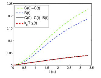
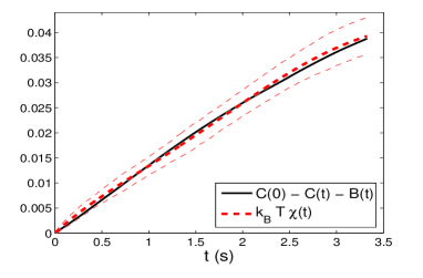
Figure 8: Experimental verification of the time-integrated form of the FDT (3.35), different terms (left), error brackets (right), from GPC (09)

III.5 Green-Kubo formula for diffusions

Let us consider a diffusion process given by the stochastic equation (1.44) with $\,X_{0t}=X_{0}+\epsilon^{a}_{t}Y_{a}\,$ and $\,X_{0},Y_{a}$,  and $\,X_{\alpha}\,$ time independent. Let $\,\nu(dx)={\rm e}^{-\varphi(x)}\lambda(dx)\,$ be the invariant measure when $\,\bm{\epsilon}=0$.  As was discussed in Lecture 1 in Sec. I.7,  a fluctuation relation

$$\mathbb{E}^{\bm{\epsilon}}_{\mu_{0}}\,{\rm e}^{-{\cal W}_{\tau}[\bm{x}]}\,=\,1$$ (3.60)

holds in this case for functional $\,{\cal W}_{\tau}\,$ given by Eqs. (1.81) and (1.89) with $\,Y_{t}(x)=\epsilon^{a}_{t}Y_{a}$.  In particular, the choice $\,\rho_{0}(x)\,={\rm e}^{-\varphi(x)}=\rho^{\prime}_{0}(x^{*})\,$ results in the expression

$${\cal W}_{\tau}[\bm{x}]\,=\,\int\limits_{0}^{\tau}\epsilon^{a}_{t}\,\big{(}(\partial_{i}\varphi)\,Y_{a}^{i}\,-\,\partial_{i}Y_{a}^{i}\big{)}(x_{t})\,dt\,\equiv\,\int\limits_{0}^{\tau}\epsilon^{a}_{t}\,{\cal J}_{a}(x_{t})\,dt\,.$$ (3.61)

Expanding Eq. (3.60) to the second order in $\,\bm{\epsilon}\,$ around $\,\bm{\epsilon}=0$,  we obtain the relation

$$-\int\limits_{0}^{\tau}\epsilon^{a}_{t}\,\,\mathbb{E}_{\nu}\,{\cal J}_{a}(x_{t})\,dt\,-\int\limits_{0}^{\tau}\epsilon^{a}_{t}\,dt\int\limits_{0}^{t}\,\epsilon^{b}_{s}\,\,\frac{\delta}{\delta\epsilon^{b}_{s}}\Big{|}_{\bm{\epsilon}=\bm{0}}\,\mathbb{E}^{\bm{\epsilon}}_{\nu}\,{\cal J}_{a}(x_{t})\,ds\hskip 25.6073pt$$ (3.62)

$$+\,\frac{{}_{1}}{{}^{2}}\,\int\limits_{0}^{\tau}\epsilon^{a}_{t}\,dt\int\limits_{0}^{\tau}\epsilon^{b}_{s}\,\,\mathbb{E}_{\nu}\,{\cal J}_{b}(x_{s})\,{\cal J}_{a}(x_{t})\,ds\,\,=\,0$$ (3.63)

or,  stripping it from the arbitrary functions $\,\bm{\epsilon}\,$ and taking $\,s\leq t$,

$$\mathbb{E}_{\nu}\,{\cal J}_{a}(x_{t})\,=\,0\,,$$ (3.64)

$$\mathbb{E}_{\nu}\,{\cal J}_{b}(x_{s})\,{\cal J}_{a}(x_{t})\,=\,\frac{\delta}{\delta\epsilon^{b}_{s}}\Big{|}_{\bm{\epsilon}=\bm{0}}\,\mathbb{E}^{\bm{\epsilon}}_{\nu}\,{\cal J}_{a}(x_{t})\,.$$ (3.65)

The first of those equations states that the stationary expectation of $\,{\cal J}_{a}\,$ vanishes. The integration of the second equation over $\,s\,$ from zero to $\,t\,$ gives

$$\int\limits_{0}^{t}\mathbb{E}_{\nu}\,{\cal J}_{b}(x_{s})\,{\cal J}_{a}(x_{t})\,ds\,=\,\partial_{\epsilon^{b}}|_{\epsilon=0}\,\mathbb{E}_{\nu}^{\epsilon}\,{\cal J}_{a}(x_{t})\,,$$ (3.66)

where on the right hand side $\,\epsilon=(\epsilon^{a})\,$ is taken time independent.  Assuming that for $\,t\to\infty\,$ the expectation

$$\mathbb{E}_{\nu}^{\epsilon}\,{\cal J}_{a}(x_{t})\ \,\mathop{\longrightarrow}\limits_{t\to\infty}\,\ \int{\cal J}_{a}(x)\,\nu_{\epsilon}(dx)\,,$$ (3.67)

where $\,\nu_{\epsilon}\,$ is the invariant measure of the stationary process with constant $\,\epsilon\,$ and using the time-translation invariance of the right hand side,  we obtain from Eq. (3.66) the relation

$$\boxed{\,\int\limits_{-\infty}^{t}\mathbb{E}_{\nu}\,{\cal J}_{b}(x_{s})\,{\cal J}_{a}(x_{t})\,ds\,=\,\partial_{\epsilon^{b}}|_{\epsilon=0}\,\int{\cal J}^{a}(x)\,\,\nu_{\epsilon}(dx)\,}\,.$$ (3.68)

This is the  Green-Kubo formula  G (54); K (57)  that permits to extract the linear-regime change of the stationary expectation of observables $\,{\cal J}_{a}(x)\,$ under a perturbation of the dynamics from their unperturbed dynamical correlation function.

If the unperturbed process is time-reversible, i.e. if $\,L={\rm e}^{\hskip 0.56917pt\varphi}L^{\dagger}{\rm e}^{-\varphi}$,  then

$$\mathbb{E}_{\nu}\,{\cal J}^{b}(x_{s})\,{\cal J}^{a}(x_{t})\,=\,\mathbb{E}_{\nu}\,{\cal J}_{a}(x_{-t})\,{\cal J}_{b}(x_{-s})\,=\,\mathbb{E}_{\nu}\,{\cal J}^{a}(x_{s})\,{\cal J}^{b}(x_{t})\,,$$ (3.69)

and we may infer from the Eq. (3.68) the Onsager reciprocity relations

$$\boxed{\,\partial_{\epsilon^{b}}|_{\epsilon=0}\,\int{\cal J}^{a}(x)\,\,\nu_{\epsilon}(dx)\,=\,\partial_{\epsilon^{a}}|_{\epsilon=0}\,\int{\cal J}^{b}(x)\,\,\nu_{\epsilon}(dx)\,}\,.$$ (3.70)

The Green-Kubo formula itself may be rewritten in this case in the symmetrized form

$$\frac{{}_{1}}{{}^{2}}\int\limits_{-\infty}^{\infty}\mathbb{E}_{\nu}\,{\cal J}^{b}(x_{s})\,{\cal J}^{a}(x_{t})\,ds\,=\,\partial_{\epsilon^{b}}|_{\epsilon=0}\,\int{\cal J}^{a}(x)\,\nu_{\epsilon}(dx)\,.$$ (3.71)

The last three relations also hold if the unperturbed process is time-reversible only relative to an involution $\,x\to x^{*}\,$ but the observables $\,{\cal J}^{a}\,$ are all either even or odd under it: $\,{\cal J}^{a}(x^{*})=\pm{\cal J}^{a}(x)\,$ with the same sign for all $\,a$.

Example 7.  Above, we considered for simplicity only perturbations of the drift term in the diffusions, but similar strategy may be applied to perturbations involving also the pure diffusion part of the dynamics. For concreteness, let us consider the anharmonic chain (1.93) of Example 5 in Sec. I.7 with $\,M_{i}^{-1}=0\,$ for $\,i\not=0,L\,$ and with $\,\beta_{0}=\beta-\frac{1}{2}\epsilon\,$ and $\,\beta_{L}=\beta+\frac{1}{2}\epsilon\,$ so that the functional (1.106) corresponding to the piecewise constant interpolation of $\,\beta_{i}\,$ is equal to

$${\cal W}_{\tau}(\bm{x})\,=\,\epsilon\int\limits_{0}^{\tau}j_{(i-1,i)}(x_{t})\,dt\,.$$ (3.72)

Expanding the Jarzynski equality (1.10) to the second order in $\,\epsilon\,$ and proceeding as before, one arrives at the identity

$$\int\limits j_{(i-1,i)}(x)\hskip 0.71114pt\,\nu(dx)\ =\ 0\,,$$ (3.73)

where $\,\nu(dx)\,$ is the Gibbs measure at inverse temperature $\,\beta\,$ for the chain,  and at the Green-Kubo relation

$$\frac{{}_{1}}{{}^{2}}\int\limits_{-\infty}^{\infty}\mathbb{E}_{\nu}\hskip 0.71114pt\,j_{(i-1,i)}(x_{s})\hskip 0.71114pt\,j_{(i-1,i)}(x_{t})\hskip 0.71114pt\,ds\ \,=\,\ \partial_{\epsilon}|_{\epsilon=0}\int\hskip 0.71114pt\,j_{(i-1,i)}(x)\,\nu_{\epsilon}(dx)\,,$$ (3.74)

where $\,\nu_{\epsilon}(dx)\,$ is the invariant nonequilibrium measure for the perturbed boundary temperatures  (the equilibrium underdamped $\,\epsilon=0\,$ dynamics is time-reversible under the involution that reverses the sign of momenta and the heat flux $\,j_{(i-1,i)}\,$ is odd under it).  One of the outstanding open problems of mathematical physics is the control of the large $\,L\,$ behavior of the thermal conductivity

$$\kappa(L,\beta)\,=\,L\hskip 0.85355pt\beta^{2}\,\partial_{\epsilon}|_{\epsilon=0}\int\hskip 0.71114pt\,j_{(i-1,i)}(x)\,\nu_{\epsilon}(dx)$$ (3.75)

giving the proportionality constant between the heat flux and the (infinitesimally small) temperature gradient imposed at the boundary. In particular, one would like to establish the conjectured Fourier law which (in a weak form) states that the limit $\,\lim\limits_{L\to\infty}\,\kappa(L,\beta)\,$ exists and is strictly positive BLR (00); BK (07).

IV Large deviations and stationary fluctuation relations

In the presence of a small parameter $\,\epsilon$,  a family $\,\mu_{\epsilon}(dX)\,$ of measures may exhibit a  large deviations regime  in which it takes an exponential form, with the inverse of the small parameter as the prefactor in front of a negative exponent. This is often formulated as the existence of a  rate function $\,{\cal I}(X)\,$ such that

$$-\,\inf\limits_{X\in A^{o}}\,I(X)\,\leq\,\liminf\limits_{\epsilon\to 0}\,\epsilon\hskip 0.71114pt\ln\mu_{\epsilon}(A)\,\leq\,\limsup\limits_{\epsilon\to 0}\,\epsilon\hskip 0.71114pt\ln\mu_{\epsilon}(A)\,\leq\,-\,\mathop{\rm inf}\limits_{X\in\bar{A}}\,I(X)\,,$$ (4.1)

where $\,A^{o}\,$ is the interior and $\,\bar{A}\,$ the closure of set $\,A$.  In less formal, terms, this may be stated as the property

$$\mu_{\epsilon}(dX)\ \ \mathop{\sim}\limits_{\epsilon\to 0}\ \ \ {\rm e}^{-\frac{1}{\epsilon}I(X)}\,\lambda(dX)$$ (4.2)

or,  if $\,\mu_{\epsilon}(dX)\,=\,\rho_{\epsilon}(X)\,\lambda(dX)$,  as the existence in a sufficiently weak sense of the limit

$$\lim\limits_{\epsilon\to 0}\ \epsilon\ln{\rho_{\epsilon}(X)}\ =\ -\,I(X)\,.$$ (4.3)

History of the large deviations theory is long as it originates in works of the founding fathers of statistical mechanics in the nineteenth century. On the probability theory side, it goes back to contributions of the Swedish mathematician Harald Cramér from the thirties of the last century. In application to stochastic processes, small parameters may have different origin. One possibility is a small noise in the stochastic differential equations (e.g. low temperature in the Langevin equations). This is the domain of application of Freidlin-Wentzell theory of large deviations FW (84). We shall encounter it below on a formal level for diffusions in a functional space. Another possibility, developed first by Donsker-Varadhan DV (75), is the long-time asymptotics of the solutions of stochastic equations, see also the textbooks DS (89); DZ (98). We shall need its version that, to my knowledge, was not explicitly considered in mathematical texts but appeared in the papers of physicists CCM (07); MNW (08). For an introduction to the subject of large deviations,  see also ref. T (11).

IV.1 Large deviations at long times

For a stationary diffusion Markov process $\,(x_{t})\,$ solving the stationary version of Eq. (1.44), define the  empirical density  and  empirical current  by the formulae

$$\rho_{\tau}(x)\,=\,\tau^{-1}\int\limits_{0}^{\tau}\delta(x-x_{t})\,dt\,,\qquad j_{\tau}(x)\,=\,\tau^{-1}\int\limits_{0}^{\tau}\delta(x-x_{t})\circ dx_{t}\,,$$ (4.4)

where, as before, “$\circ$” signifies the Stratonovich convention. Assuming the ergodicity of the process, when $\,\tau\to\infty$, $\,\rho_{\tau}\,$ converges (in a weak sense) to the density $\,\rho\,$ of the invariant measure $\,\nu(dx)=\rho(x)\,\lambda(dx)$,  and $\,j_{\tau}\,$ converges to the probability current $\,j\,$ given by

$$j(x)\,=\,\big{(}\widehat{X}_{0}(x)\,-\,{\cal D}(x)\nabla\big{)}\rho(x)\,\equiv\,j_{\rho}(x)\,.$$ (4.5)

see Eq. (1.48),  which is conserved:

$$\nabla\cdot j(x)\,=\,0\,.$$ (4.6)

We would like to inquire about the asymptotics of that convergence. The answer is provided by the large deviations form of the joint distribution function of the empirical density $\,\rho_{\tau}\,$ and current $\,j_{\tau}$:

$$\mathbb{E}_{\nu}\,\delta[\varrho-\rho_{\tau}]\,\,\delta[\jmath-j_{\tau}]\ \,\mathop{\sim}\limits_{\tau\to\infty}\,\ {\rm e}^{-\tau{\cal I}[\varrho,\jmath]}\,,$$ (4.7)

with the rate function

$${\cal I}[\varrho,\jmath]\,=\,\begin{cases}\,\infty\hskip 179.53682pt{\rm if}\qquad\nabla\cdot\jmath\not=0\,,\cr\cr\frac{{}_{1}}{{}^{4}}\int\big{[}\big{(}\jmath-j_{\varrho}\big{)}\cdot(\varrho\hskip 0.56917pt{\cal D})^{-1}\big{(}\jmath-j_{\varrho}\big{)}\big{]}(x)\,\lambda(dx)\qquad{\rm if}\qquad\nabla\cdot\jmath=0\,,\end{cases}$$ (4.8)

where $\,j_{\varrho}\,$ is given by Eqs. (4.5) with $\,\rho\,$ replaced by $\,\varrho$.  The large-deviations asymtotics for empirical densities or empirical currents only is then obtained by the “contraction principle”:

$$\mathbb{E}_{\nu}\,\,\delta[\varrho-\rho_{\tau}]\ \,\mathop{\sim}\limits_{\tau\to\infty}\ {\rm e}^{-\tau{\cal I}[\varrho]}\,,\qquad\mathbb{E}_{\nu}\,\,\delta[\jmath-j_{\tau}]\ \,\mathop{\sim}\limits_{\tau\to\infty}\ {\rm e}^{-\tau{\cal I}[\jmath]}$$ (4.9)

with

$${\cal I}[\varrho]\,=\,\mathop{\rm min}\limits_{\jmath}\,{\cal I}[\varrho,\jmath]\,,\qquad{\cal I}[\jmath]\,=\,\mathop{\rm min}\limits_{\varrho}\,{\cal I}[\varrho,\jmath]$$ (4.10)

in a slightly abusive notation. The first minimum may be rewritten (why?) in terms of a maximum over Lagrange multipliers $\,f(x)$:

$${\cal I}[\varrho] = -\,\mathop{\rm min}\limits_{f}\,\int(\nabla f)(x)\cdot\big{[}\varrho\hskip 0.56917pt{\cal D}(\nabla f)+j_{\varrho}\big{]}(x)\,\lambda(dx)$$ (4.11)

$$= -\,\frac{{}_{1}}{{}^{4}}\int\big{[}(\nabla\cdot j_{\varrho})(\nabla\cdot\varrho\hskip 0.56917pt{\cal D}\nabla)^{-1}(\nabla\cdot j_{\varrho})\big{]}(x)\,\lambda(dx)\,.$$ (4.12)

Note that $\,{\cal I}[\varrho]\,$ is non-negative and attains its vanishing minimum on the density $\,\rho\,$ of the invariant measure such that $\,\nabla\cdot j_{\rho}=0$.  The first line of Eq. (4.12) may be also rewritten as

$${\cal I}[\varrho] = -\,\mathop{\rm min}\limits_{f}\,\int\big{[}(\nabla f)\cdot\varrho\hskip 0.56917pt{\cal D}(\nabla f)+f\,L^{\dagger}\varrho\big{]}(x)\,\lambda(dx)$$ (4.13)

$$= -\,\mathop{\rm min}\limits_{u>0}\,\int\big{(}u^{-1}Lu\big{)}(x)\,\varrho(x)\,\lambda(dx)\,,$$ (4.14)

where the last minimum is over positive functions $\,u(x)={\rm e}^{f(x)}$.  In the last form, the formula for the rate function $\,{\cal I}[\varrho]\,$ holds for general continuous-time stationary Markov processes DV (75).

As for the rate function $\,{\cal I}(\jmath)$,  note that $\,{\cal I}[\varrho,\jmath]\,$ is a local nonlinear functional of the density $\,\varrho>0\,$ constrained to be normalized, quadratic in its first derivatives, leading to the $2^{\rm nd}$-order differential equation for the extrema. Even in one dimension where the latter equation reduces to an ODE and $\,\nabla\cdot\jmath=0\,$ means that $\,\jmath={\rm const}.$,   the minimization over $\,\varrho\,$ cannot be explicitly solved analytically. Nevertheless, for weak noise, one may resort to semiclassical instanton-gas type expansions which go back to ideas of Kramers from the 40’s of the last century and to Freidlin-Wentzell large deviations theory, and which are still being actively developed, see e.g. E (06); CCM (09).

Example 8.  For the one-dimensional diffusion defined by Eqs. (3.51), (3.52) and (3.53), the drift has two zeros, one unstable at $\,\theta_{u}\approx 0.214\,rad\,$ and one stable at $\,\theta_{s}=2\pi-\theta_{u}$.  One obtains in this case the instantonic expression CCM (09)

$${\cal I}(\jmath)\,\approx\,-\,\jmath\,\ln{\frac{\sqrt{\jmath^{2}+4\kappa_{+}\kappa_{-}}-\jmath}{2\kappa_{-}}}\,-\,\sqrt{\jmath^{2}+4\kappa_{+}\kappa_{-}}\,+\,\kappa_{+}+\kappa_{-}$$ (4.15)

for $\kappa_{+}=A_{0}\exp[D^{-1}\,A_{-}]$, $\,\kappa_{-}=A_{0}\exp[-D^{-1}A_{+}]\,$ where $\,A_{-}\,$ is the (tiny negative) area under the negative part of the drift graph, $\,A_{+}\,$ is the one under the positive part of the graph, see the left plot in FIG. 8, and $\,A_{0}=M\sqrt{|(\partial_{\theta}^{2}U)(\theta_{s})(\partial_{\theta}^{2}U)(\theta_{u})|}/(2\pi)$.  The most probable value of $\,j_{\tau}\,$ for small $\,D\,$ is $j=\kappa_{+}-\kappa_{-}$.  The same large deviation function (4.15) may be obtained from a jump process with plus or minus jumps occurring with rates $\,\kappa_{\pm}\,$ by looking at the statistics of the large sums of jumps LS (99). Those jumps correspond in the diffusion to the tunneling to the right and to the left through the barriers separating the stable and unstable points of the drift.

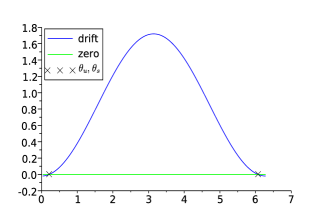
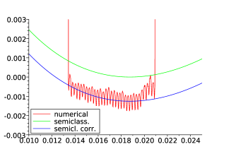
Figure 9: Drift in Eq. (3.51) (left) and the comparison of numerical and theoretical rate functions for the empirical current (right)

The large deviations statistics of the empirical current $\,j_{\tau}$,  that is $\,\theta$-independent in this regime, may be extracted from the one of its spatial mean

$$\frac{{}_{1}}{{}^{2\pi}}\int\limits_{0}^{2\pi}j_{\tau}(\theta)\,\lambda(d\theta)\,=\,\frac{{}_{1}}{{}^{2\pi\tau}}\int\limits_{0}^{\tau}d\theta_{t}$$ (4.16)

The numerical simulation of the minus logarithm of the distribution function of the latter divided by $\,\tau=4167\,s\,$ is shown on the right plot in FIG. 8. Note its oscillatory character (with the period $1/\tau$). Its plot averaged over the oscillations compares well on the interval with sufficient number of events with the semiclassical formula (4.15) shifted by $\,-(2\tau)^{-1}\ln\big{(}\frac{\partial^{2}_{\jmath}{\cal I}(\kappa_{+}-\kappa_{-})}{2\pi}\big{)}\,$ to include the one-loop correction. I do not know whether the convergence (4.3) (for $\,X=\jmath\,$ and $\,\epsilon=\tau^{-1}$)  holds here pointwise or only after smearing with test functions.

IV.2 Gallavotti-Cohen type fluctuation relation

Defining the time-reversed diffusion process one of the ways described in Sec. I.7 and using relation (1.8), we obtain the identity

$$\mathbb{E}_{\nu}\,\,{\rm e}^{-{\cal W}}\,{\cal F}(\rho_{\tau},j_{\tau})\,=\,\mathbb{E}^{\prime}_{\nu^{\prime}}\,\,{\cal F}(\rho^{*}_{\tau},-j^{*}_{\tau})\,,$$ (4.17)

where, by definition,

$$\rho^{*}_{\tau}[\bm{x}]\,=\,\rho_{\tau}[\bm{x}^{*}]\,,\qquad j^{*}_{\tau}[\bm{x}]\,=\,-\,j_{\tau}[\bm{x}^{*}]$$ (4.18)

(the minus sign in the transformation of the current comes from the change of the sign of the time derivative of the process under the time reversal).  An easy calculation shows that in their dependence on points in space, $\,\rho^{*}_{\tau}\,$ and $\,j^{*}_{\tau}\,$ are related to empirical density $\,\rho_{\tau}\,$ and empirical current $\,j_{\tau}\,$ of Eqs. (4.4) by the geometric transformation rule for densities and currents:

$$\varrho^{*}(x^{*})\,\frac{\partial(x^{*})}{\partial(x)}\,=\,\varrho(x)\,,\qquad\jmath^{*}(x^{*})\,\frac{\partial(x^{*})}{\partial(x)}\,=\,\frac{\partial x^{*}}{\partial x}\,\jmath(x)\,,$$ (4.19)

with $\,\frac{\partial x^{*}}{\partial x}\,$ denoting the Jacobi matrix and $\,\frac{\partial(x^{*})}{\partial(x)}\,$ the Jacobian of the involution $\,x\mapsto x^{*}$.  On the other hand,  by Eq. (1.81) and (1.82),

$${\cal W}\,=\,-\ln\rho^{\prime}(x_{\tau}^{*})\,+\,\tau\,{\omega}[\rho_{\tau},j_{\tau}]\,+\,\ln\rho_{0}(x_{0})\,,$$ (4.20)

where

$${\omega}[\varrho,\jmath]\,=\,\int\Big{[}\widehat{X}^{+}_{0}\cdot{\cal D}^{-1}\big{(}\jmath-X^{-}_{0}\varrho\big{)}\,-\,(\nabla\cdot X^{-}_{0})\,\varrho\Big{]}(x)\,\lambda(dx)$$ (4.21)

so that

$$\int\limits_{0}^{\tau}{\cal J}_{t}\,dt\,=\,\tau\,{\omega}[\rho_{\tau},j_{\tau}]\,.$$ (4.22)

Comparing the large $\,\tau\,$ asymptotics on both sides of identity (4.17) we infer the identity

$$\boxed{\,{\cal I}[\varrho,\jmath]\,+\,{\omega}[\varrho,\jmath]\,=\,{\cal I}^{\prime}[\varrho^{*},-\jmath^{*}]\,}$$ (4.23)

where $\,\varrho^{*}\,$ and $\,\jmath^{*}\,$ are defined by the relations (4.19). This is the stationary fluctuation relation for the rate functions describing the large deviations of empirical density and current for the direct and time-reversed diffusion process. A simple exercise using Eqs. (4.8) and the identity

$$j^{\prime*}_{\varrho^{*}}\,=\,j_{\varrho}-2X^{-}_{0}\varrho\,=\,-\,j_{\varrho}+2\widehat{X}^{+}_{0}\varrho-2{\cal D}\nabla\varrho\,,$$ (4.24)

where $\,j^{\prime}_{\rho}\,$ defined by Eq. (4.5) but for the time-reversed process, permits to verify Eq. (4.23) directly. The probability distribution of the quantity $\,\omega[\rho_{\tau},j_{\tau}]\,$ given by Eq. (4.22), representing the rate of the entropy production in environment in the units of $\,k_{B}$,  has also a large deviations regime with the rate function given by the contraction

$${\cal I}(\varpi)\ =\,\mathop{\rm min}\limits_{{\omega}[\varrho,\jmath]=\varpi}\,{\cal I}[\varrho,\jmath]\,.$$ (4.25)

From Eq. (4.23), using also the relation

$${\omega}^{\prime}[\rho^{*},-\jmath^{*}]=-\,{\omega}[\varrho,\jmath]\,,$$ (4.26)

where $\,\omega^{\prime}\,$ corresponds to the time-reversed process,  a consequence of the second equality in (1.81),  we obtain immediately the fluctuation relation

$$\boxed{\,{\cal I}(\varpi)\,+\,\varpi\,=\,{\cal I}^{\prime}(-\varpi)\,}\,.$$ (4.27)

The latter identity holds, in particular, for the time reversal with $\,\widehat{X}^{+}_{0}=0\,$ considered in the case ${\bf(d)}$ of Sec. I.7. In this instance,

$${\omega}[\rho_{\tau},j_{\tau}]\,=\,-\int(\nabla\cdot X_{0}^{-})(x)\,\rho_{\tau}(x)\,\lambda(dx)\,=\,-\,\tau^{-1}\int\limits_{0}^{\tau}(\nabla\cdot X_{0}^{-})(x_{t})\,dt\,\equiv\,{\omega}[\rho_{\tau}]\,,$$ (4.28)

which reduces to the phase-space contraction rate in the deterministic case with $\,X_{\alpha}\equiv 0\,$ and $\,X^{-}_{0}=X_{0}$.  The stationary fluctuation relation (4.27) for uniformly hyperbolic deterministic dynamical systems (in the case when the time-reversed dynamics coincides with the direct one) was proven in GC95a ; GC95b ) as the  Fluctuation Theorem.  The existence of large deviations regime for $\,{\omega}[\rho_{\tau}]\,$ representing the phase-space contraction rate followed in that case from the thermodynamical formalism for such dynamical systems so that the Fluctuation Theorem of Gallavotti-Cohen is not a direct consequence of the relation (4.27) for the stochastic diffusions. In the latter case, we could obtain (4.27) from the transient fluctuation relation (4.17) holding for the stationary dynamics on any time interval, whereas there is no such relation for the general stationary deterministic systems that typically have singular invariant measures. The transient Evans-Searles relation for such systems employs the non-invariant smooth initial measures and a non-trivial work using the thermodynamical formalism would be needed to show that they lead for long times to the Gallavotti-Cohen relation.

The fluctuation relation (4.27) with $\,{\cal I}^{\prime}={\cal I}\,$ should also hold for the large-deviations rate function of the cumulated heat flux $\,{\cal W}_{\tau}\,$ given by Eqs. (1.103), (1.105) or (1.106) in the non-equilibrium stationary state of the anharmonic chain with Hamiltonian dynamics in the interior that we discussed in Example 5 in Sec. I.7), see RT (02) for a proof of this fact for a closely related model.

IV.3 Large deviations for replicated diffusions

The final part of these lectures is based on a joint work in progress with F. Bouchet et C. Nardini BGN . The first half concerning the large deviations for independent replicated systems is rather well known, but we present it in the spirit of the  macroscopic fluctuation theory  developed for the dynamics of boundary driven lattice gases in a series of papers of the Rome group, see e.g. BDG (06). The second half that develops the macroscopic fluctuation theory for a non-equilibrium system of replicated diffusions with a mean-field interaction seems original.

Let us consider $\,N\,$ independent copies $\,(x^{n}_{t}),\ n=1,\dots,N$,  of identical diffusions satisfying stochastic equation (1.44). For such replicated system, we may define the dynamical empirical density and empirical current by the formulae

$$\bm{\rho}_{N}(t,x)\,=\,\frac{1}{N}\sum\limits_{n=1}^{N}\delta(x-x^{n}_{t})\,,\qquad\bm{j}_{N}(t,x)\,=\,\frac{1}{N}\sum\limits_{n=1}^{N}\delta(x-x^{n}_{t})\circ\frac{dx^{n}_{t}}{dt}\,.$$ (4.29)

Here and below, we use bold letters for quantities that depend on time and (phese-)space coordinates. We shall also employ the notation $\,\rho_{Nt}(x)\,$ and $\,j_{Nt}(x)\,$ whenever we consider only the $\,x$-dependence for fixed $\,t$.  Note the continuity equation

$$\partial_{t}\bm{\rho}_{N}\,+\,\nabla\cdot\bm{j}_{N}\,=\,0\,.$$ (4.30)

Let $\,\varPhi[\varrho]\,$ be a functional of (possibly distributional) densities of the cylindrical form:

$$\varPhi[\varrho]\,=\,f\Big{(}\int h_{1}(x_{1})\,\rho(x_{1})\,\lambda(dx_{1}),\cdots,\int h_{k}(x_{k})\,\varrho(x_{k})\,\lambda(dx_{k})\Big{)}\,.$$ (4.31)

In its $t$-dependence, random variable $\,\varPhi(\rho_{Nt})\,$ satisfies the stochastic equation

$$d\varPhi[\rho_{Nt}]\ =\ \int\frac{\delta\varPhi[\rho_{Nt}]}{\delta\varrho(x)}\Big{(}-\frac{{}_{1}}{{}^{N}}\sum\limits_{n}(\nabla\delta)(x-x^{n}_{t})\big{(}X_{0t}(x^{n}_{t})\,dt+X_{\alpha t}(x^{n}_{t})\circ dW_{\alpha}^{n}(t)\big{)}\Big{)}\,\lambda(dx)$$ (4.32)

$$=\ \int\Big{(}\rho_{Nt}\,X_{0t}\nabla\frac{\delta\varPhi[\rho_{Nt}]}{\delta\varrho}\Big{)}(x)\,\lambda(dx)\,dt\,+\,\frac{{}_{1}}{{}^{N}}\sum\limits_{n}X_{\alpha}(x^{n}_{t})\Big{(}\nabla\frac{\delta\varPhi[\rho_{Nt}]}{\delta\varrho}\Big{)}(x^{n}_{t})\circ dW_{\alpha}^{n}(t)$$ (4.33)

which implies that

$$\frac{d}{dt}\ \underline{\mathbb{E}}_{\underline{\nu}}\ \varPhi[\rho_{Nt}]\ =\ \underline{\mathbb{E}}_{\underline{\nu}}\,\bigg{[}\int\Big{(}j_{\rho_{Nt}}\nabla\frac{\delta\varPhi[\rho_{Nt}]}{\delta\varrho}\Big{)}(x)\,\lambda(dx)$$ (4.34)

$$+\ \frac{{}_{1}}{{}^{N}}\int\rho_{Nt}(x)\,{\cal D}^{ij}_{t}(x)\,\delta(x-y)\,\nabla_{x^{i}}\nabla_{y^{j}}\frac{\delta^{2}\varPhi[\rho_{Nt}]}{\delta\varrho(x)\,\delta\varrho(y)}\,\lambda(dx)\lambda(dy)\ \equiv\ \underline{\mathbb{E}}_{\underline{\nu}}\ \big{(}{\cal L}_{Nt}\varPhi\big{)}[\rho_{Nt}]\bigg{]}\,,\qquad$$ (4.35)

where $\,\underline{\mathbb{E}}_{\underline{\nu}}\,$ denotes the expectation value over the replicated processes and $\,j_{\rho_{t}}\,$ is given by Eq. (1.48). Note that the $2^{\rm nd}$-order term in the functional operator $\,{\cal L}_{Nt}\,$ is proportional to $\,\frac{1}{N}$.  Formally, this is the same equation as the one for the expectation of the diffusion process in the space of densities solving the stochastic PDE

$$\partial_{t}\bm{\rho}\,+\,\nabla\cdot\bm{j}_{\bm{\rho},\bm{\xi}}\,=\,0$$ (4.36)

where

$$\bm{j}_{\bm{\rho},\bm{\xi}}\,=\,\bm{j}_{\bm{\rho}}\,+\,(2N^{-1}\bm{\rho}\bm{{\cal D}})^{1/2}\bm{\xi}$$ (4.37)

with the space-time white noise $\,\bm{\xi}$,

$$\mathbb{E}\,\,\bm{\xi}^{i}(t,x)\,=\,0\,,\qquad\mathbb{E}\,\,\bm{\xi}^{i}(t,x)\,\bm{\xi}^{j}(s,y)\,=\,\delta^{ij}\,\delta(t-s)\,\delta(x-y)\,.$$ (4.38)

Compare Eq. (4.36) to the continuity equation (4.30). In the limit $\,N\to\infty$,  Eq. (4.36) reduces to the standard Fokker-Plank equation

$$\partial_{t}\bm{\rho}+\nabla\cdot\bm{j}_{\bm{\rho}}\,=\,0\,,$$ (4.39)

for the instantaneous probability densities of a single copy of the process, see Eqs. (1.47) and (1.48).

IV.4 Hamilton-Jacobi equation and Sanov Theorem

The probability distributions of the empirical densities $\,\rho_{Nt}\,$ evolve by the adjoint operator $\,{\cal L}_{Nt}^{*}\,$ and their hypothetical densities by the formal adjoint $\,{\cal L}_{Nt}^{\dagger}\,$ built with the use of the rule

$$\Big{(}\frac{\delta}{\delta\varrho}\Big{)}^{\dagger}\,=\,-\,\frac{\delta}{\delta\varrho}\,.$$ (4.40)

In particular, assuming that those densities have the large-deviation form $\,{\rm e}^{-N{\cal F}_{t}[\varrho]}\,$,  we obtain in the leading order the  Hamilton-Jacobi equation  for $\,{\cal F}_{t}$:

$$\boxed{\,\partial_{t}{\cal F}_{t}[\varrho]\,+\,\int\bigg{(}\Big{(}\nabla\frac{\delta{\cal F}_{t}[\varrho]}{\delta\varrho}\Big{)}\cdot\varrho\hskip 0.56917pt{\cal D}_{t}\Big{(}\nabla\frac{\delta{\cal F}_{t}[\varrho]}{\delta\varrho}\Big{)}\,+\,j_{\varrho\hskip 0.56917ptt}\cdot\nabla\frac{\delta{\cal F}_{t}[\varrho]}{\delta\varrho}\bigg{)}(x)\,\lambda(dx)\,=\,0\,}$$ (4.41)

We shall call $\,{\cal F}_{t}[\rho]\,$ the free energy of the replicated system. Eq. (4.41) is solved by the relative entropy functional in the units of $\,k_{B}$

$$\boxed{\,{\cal F}_{t}[\varrho]\,=\,\int\Big{(}\varrho\,\ln\big{(}\frac{\varrho}{\rho_{t}}\big{)}\Big{)}(x)\,\lambda(dx)\,=\,k_{B}^{-1}S[\varrho\|\rho_{t}]\,}$$ (4.42)

where $\,\rho_{t}\,$ solves the Fokker-Planck equation (4.39).

Theorem  (Dynamical version of the Sanov Theorem).

The solution (4.42) of the Hamilton-Jacobi equation (4.41) describes the time evolution of the rate function for the large deviations of the distribution of empirical density $\,\rho_{Nt}\,$ if the initial points $\,x^{n}_{0}\,$ of the replicated processes are distributed (independently) with the probability density $\,\rho_{0}$.

Corollary.  In the particular case of the replicated stationary diffusion process, the distribution of the empirical densities $\,\rho_{Nt}\,$ stays time independent and for large $\,N\,$ it takes the large deviations form with the rate function

$$\boxed{\,{\cal F}[\varrho]\,=\,k_{B}^{-1}S[\varrho\|\rho]\,}$$ (4.43)

where $\,\rho\,$ is the density of the invariant measure of the process. $\,{\cal F}[\varrho]\,$ solves the stationary Hamilton-Jacobi equation

$$\boxed{\,\int\bigg{(}\Big{(}\nabla\frac{\delta{\cal F}[\varrho]}{\delta\varrho}\Big{)}\cdot\varrho\hskip 0.56917pt{\cal D}\Big{(}\nabla\frac{\delta{\cal F}[\varrho]}{\delta\varrho}\Big{)}\,+\,j_{\varrho}\cdot\nabla\frac{\delta{\cal F}[\varrho]}{\delta\varrho}\bigg{)}(x)\,\lambda(dx)\,=\,0\,}\,.$$ (4.44)

Introducing the stationary current velocity in the space of densities by the formula

$${\cal V}[\varrho]\,=\,-\nabla\cdot\Big{(}j_{\varrho}\,+\,\varrho\hskip 0.56917pt{\cal D}\nabla\frac{\delta{\cal F}[\varrho]}{\delta\varrho}\Big{)}\,,$$ (4.45)

the stationary Hamiltonian-Jacobi equation (4.44) may be rewritten as the orthogonality condition

$$\int\frac{\delta{\cal F}[\varrho]}{\delta\varrho(x)}\,{\cal V}[\varrho](x)\,\lambda(dx)\,=\,0\,.$$ (4.46)

For the time reversal corresponding of case ${\bf(a)}$ in Sec. I.7,  one obtains from Eq. (4.24) the relation

$$j^{\prime*}_{\varrho^{*}}\,=\,-\,j_{\varrho}-2\varrho{\cal D}\nabla\varphi-2{\cal D}\nabla\varrho$$ (4.47)

which may be rewritten in the form

$$\boxed{\,j^{\prime*}_{\varrho^{*}}\,=\,-\,j_{\varrho}\,-\,2\hskip 0.56917pt\rho\hskip 0.56917pt{\cal D}\nabla\frac{\delta{\cal F}[\varrho]}{\delta\varrho}\,}\,.$$ (4.48)

A comparison with Eq. (4.45) yields the relations:

$${\cal V}[\varrho]\,=\,\nabla\cdot\Big{(}j^{\prime*}_{\varrho^{*}}\,+\,\varrho\hskip 0.56917pt{\cal D}\nabla\frac{\delta{\cal F}[\varrho]}{\delta\varrho}\Big{)}$$ (4.49)

and

$${\cal V}[\varrho]\,=\,\frac{{}_{1}}{{}^{2}}\,\big{(}\nabla\cdot j^{\prime*}_{\varrho^{*}}-\nabla\cdot j_{\varrho}\big{)}\,.$$ (4.50)

Example 9.  For the diffusion on a circle (3.51),

$${\cal F}[\varrho]\,=\,\int\limits_{0}^{2\pi}\varrho(\theta)\big{(}\ln{\varrho(\theta)}+\varphi(\theta)\big{)}\,\lambda(d\theta)$$ (4.51)

with $\,\varphi(\theta)\,$ given by Eq. (3.55).  In particular,  in the equilibrium case with $\,F=0$,

$${\cal F}[\varrho]\,=\,\int\limits_{0}^{2\pi}\varrho(\theta)\Big{(}\ln{\varrho(\theta)}\,+\,\beta\hskip 0.56917ptU(\theta)\Big{)}\,\lambda(d\theta)\ +\ {\rm const.}$$ (4.52)

so that $\,{\cal F}\,$ is equal in this instance to $\,\beta\,\,$ times the free energy of the gas of noninteracting particles in the thermal equilibrium at inverse temperature $\,\beta$.  Quantity $\,\varrho\,$ is the density of the gas and $\,U\,$ is the external potential.  For the Langevin equation (3.51) (with any $F$),

$$j_{\varrho}(\theta)\,=\,M\big{(}F-(\partial_{\theta}U)(\theta)\big{)}\hskip 0.56917pt\varrho(\theta)-D\hskip 0.85355pt\partial_{\theta}\varrho(\theta)\,,$$ (4.53)

and for the time reversed one of Eq. (3.59),

$$j^{\prime*}_{\varrho^{*}}(\theta)\,=\,j^{\prime}_{\varrho}(\theta)\,=\,\big{(}M(F-(\partial_{\theta}U)(\theta))-2v(\theta)\big{)}\hskip 0.56917pt\varrho(\theta)-D\hskip 0.85355pt\partial_{\theta}\varrho(\theta)\,,$$ (4.54)

where the current velocity $\,v(\theta)\,$ is given by Eq. (3.57).  In this case

$${\cal V}[\varrho](\theta)\,=\,-\partial_{\theta}\big{(}\varrho\,v\big{)}(\theta)\,.$$ (4.55)

IV.5 Dynamical large deviations for the replicated process

One can show, at least formally, that the joint distribution of the dynamical empirical density $\,\bm{\rho}_{N}\,$ and current $\,\bm{j}_{N}\,$ exhibits for large $\,N\,$ the large-deviations regime with the rate function

$${\cal I}[\bm{\varrho},\bm{\jmath}]\,=\,\begin{cases}\infty\hskip 196.60864pt{\rm if}\qquad\partial_{t}\bm{\varrho}+\nabla\cdot\bm{\jmath}\not=0\,,\cr\cr\frac{{}_{1}}{{}^{4}}\int\big{[}(\bm{\jmath}-\bm{j}_{\bm{\varrho}}\cdot(\bm{\varrho}\bm{{\cal D}})^{-1}(\bm{\jmath}-\bm{j}_{\bm{\varrho}})\big{]}(t,x)\,dt\lambda(dx)\qquad{\rm if}\qquad\partial_{t}\bm{\varrho}+\nabla\cdot\bm{\jmath}=0\,.\end{cases}$$ (4.56)

Note the similarities and the differences with the long-time rate function  (4.8).  In the formal argument using functional integrals, we shall replace $\,\bm{\rho}_{N}\,$ and $\,\bm{j}_{N}\,$ that satisfy Eq. (4.30) by $\,\bm{\rho}\,$ and $\,\bm{j}_{\bm{\rho},\bm{\xi}}\,$ connected by Eq. (4.36). Thus

$$\mathbb{E}\ \varPsi[\bm{\rho}_{N},\bm{j}_{N}]\,=\,\mathbb{E}\int\varPsi[\bm{\varrho},\bm{j}_{\bm{\varrho},\bm{\xi}}]\ \delta[\partial_{t}\bm{\varrho}+\nabla\cdot\bm{j}_{\bm{\varrho},\bm{\xi}}]\,\det\Big{(}\frac{\delta(\partial_{t}\bm{\varrho}+\nabla\cdot\bm{j}_{\bm{\varrho},\bm{\xi}})}{\delta\bm{\varrho}}\Big{)}\,D\bm{\varrho}$$ (4.57)

$$=\ \mathbb{E}\int\varPsi[\bm{\varrho},\bm{\jmath}]\,\,{\rm e}^{\,i\int\bm{a}\cdot(\bm{\jmath}-j_{\bm{\varrho},\bm{\xi}})}\,\delta[\partial_{t}\bm{\varrho}+\nabla\cdot\bm{\jmath}]\,\,D\bm{a}\,D\bm{\varrho}\,D\bm{\jmath}\,,$$ (4.58)

where we dropped the determinant which will not contribute to the large deviations (and is equal to $1$ if properly regularized). Averaging over the white noise $\,\bm{\xi}$,  we obtain:

$$\mathbb{E}\ \varPsi[\bm{\rho}_{N},\bm{j}_{N}] = \int\varPsi[\bm{\varrho},\bm{\jmath}]\ {\rm e}^{\,i\int\bm{a}\cdot(\bm{\jmath}-\bm{j}_{\bm{\varrho}})-\frac{1}{N}\int\bm{a}\cdot\bm{\varrho}\bm{{\cal D}}\,\bm{a}}\,\delta[\partial_{t}\bm{\varrho}+\nabla\cdot\bm{j}]\,\,D\bm{a}\,D\bm{\varrho}\,D\bm{\jmath}$$ (4.59)

$$= \int\varPsi[\bm{\varrho},\bm{\jmath}]\ {\rm e}^{-\frac{N}{4}\int(\bm{\jmath}-\bm{j}_{\bm{\varrho}})\cdot(\bm{\varrho}\bm{{\cal D}})^{-1}(\bm{\jmath}-\bm{j}_{\bm{\varrho}})}\,\delta[\partial_{t}\bm{\varrho}+\nabla\cdot\bm{j}]\,\,D\bm{\varrho}\,D\bm{\jmath}\,.$$ (4.60)

From the last functional integral expression, we read off the large deviations rate function (4.56) (a similar functional-integration argument may be used to obtain formula (4.8)).

The rate functions for the dynamical large deviations of the empirical density $\,\bm{\rho}_{N}\,$ alone or for the empirical current $\,\bm{\jmath}_{N}\,$ alone are given by the contraction:

$${\cal I}[\bm{\varrho}] = \mathop{\min}\limits_{\bm{\jmath}}\ {\cal I}[\bm{\varrho},\bm{\jmath}]\,=\,\frac{{}_{1}}{{}^{4}}\int\Big{[}\big{(}\partial_{t}\bm{\varrho}+\nabla\cdot\bm{j}_{\bm{\varrho}}\big{)}\big{(}-\nabla\cdot\bm{\varrho}\hskip 0.56917pt\bm{{\cal D}}\hskip 0.85355pt\nabla\big{)}^{-1}\big{(}\partial_{t}\bm{\varrho}+\nabla\cdot\bm{j}_{\bm{\varrho}}\big{)}\Big{]}(t,x)\,dt\lambda(dx)\,,\qquad$$ (4.61)

$${\cal I}[\bm{\jmath}] = \mathop{\min}\limits_{\bm{\varrho}}\ {\cal I}[\bm{\varrho},\bm{\jmath}]\,,$$ (4.62)

with no closed expression in the latter case where an appropriate initial conditions for $\,\bm{\varrho}\,$ should be specified. As for the first formula, it follows by a formal application of the Freidlin-Wentzell theory to the diffusion (4.36) with noise (4.37) and it was rigorously established in DG (87).

We shall denote by $\,{\cal I}_{A}[\bm{\varrho},\bm{\jmath}]\,$ the rate functions given by Eq. (4.56) with the time-integral restricted to the interval $A$.  The functionals $\,{\cal I}_{[0,\tau]}(\bm{\varrho},\bm{\jmath})\,$ and $\,{\cal I}^{\prime}_{[0,\tau]}[\bm{\varrho},\bm{\jmath}]\,$ for the replicated direct and time reversed process, the latter obtained with the use of one of the rules of Sec. I.7, satisfy the stationary fluctuation relation

$$\boxed{\,{\cal I}_{[0,\tau]}[\bm{\varrho},\bm{\jmath}]\,+\,{\omega}_{[0,\tau]}[\bm{\varrho},\bm{\jmath}]\,=\,{\cal I}^{\prime}_{[0,\tau]}[\bm{\varrho}^{*},-\bm{\jmath}^{*}]\,}$$ (4.63)

where

$$\bm{\varrho}^{*}(t,x)\,=\,\bm{\varrho}(t^{*},x^{*})\,\frac{\partial(x^{*})}{\partial(x)}\,,\qquad\bm{\jmath}^{*}(t,x)\,=\,\frac{\partial x}{\partial x^{*}}\,\jmath(t^{*},x^{*})\,\frac{\partial(x^{*})}{\partial(x)}\,,$$ (4.64)

and

$${\omega}_{[0,\tau]}[\bm{\varrho},\bm{\jmath}] = \int\limits_{0}^{\tau}dt\int\Big{[}{\widehat{X}}^{+}_{0t}\cdot{\cal D}_{t}^{-1}\big{(}\jmath_{t}-X^{-}_{0t}\hskip 0.56917pt\varrho_{t}\big{)}\,-\,(\nabla\cdot X^{-}_{0t})\hskip 0.56917pt\varrho_{t}\Big{]}(x)\,\lambda(dx)$$ (4.65)

$$- \int\varrho_{t}(x)\,\ln{\varrho_{t}}(x)\,\lambda(dx)\,\bigg{|}^{\tau}_{0}\,,$$ (4.66)

compare to relations (4.23), (4.19) and (4.21). These identities follow in a straightforward way from the relations

$$\bm{j}^{\prime*}_{\bm{\varrho}^{*}}\,=\,\bm{j}_{\bm{\varrho}}-2\bm{X}^{-}_{0}\bm{\varrho}\,=\,-\bm{j}_{\bm{\varrho}}+2\widehat{\bm{X}}^{+}_{0}\bm{\varrho}-2\bm{{\cal D}}\nabla\bm{\varrho}$$ (4.67)

that generalize Eqs. (4.24). In the particular case of the stationary process and the time reversal corresponding of case ${\bf(a)}$ in Sec. I.7,

$${\omega}_{[0,\tau]}[\bm{\varrho},\bm{\jmath}]\,=\,{\cal F}[\varrho_{0}]-{\cal F}[\varrho_{\tau}]\,.$$ (4.68)

By contraction, we infer then from relation (4.64) the identity

$$\boxed{\,{\cal I}_{[0,\tau]}[\bm{\varrho}]\,+\,{\cal F}[\varrho_{0}]-{\cal F}[\varrho_{\tau}]=\,{\cal I}^{\prime}_{[0,\tau]}[\bm{\varrho}^{*}]\,}$$ (4.69)

Let $\,\varrho_{0}=\rho$,  where $\,\rho={\rm e}^{-\varphi}\,$ is the invariant density of the single process, so that $\,{\cal F}[\varrho_{0}]=0\,$ follows.  Take $\,\tau\to\infty$. Then the minimum of the right hand side over $\,\bm{\varrho}^{*}\,$ with $\,\varrho_{0}\,$ and $\,\varrho_{\infty}\,$ fixed is realized by the trajectory $\,\bm{\varrho}^{\prime}\,$ solving the reversed process Fokker-Planck equation

$$\partial_{t}\bm{\varrho}^{\prime}+\nabla\cdot\bm{j}^{\prime}_{\bm{\varrho}^{\prime}}\,=\,0$$ (4.70)

that relaxes from $\,(\varrho_{\infty})^{*}\,$ to the invariant density $\,\rho^{*}\,$ and $\,{\cal I}^{\prime}_{[0,\infty[}(\bm{\varrho}^{\prime})\,$ vanishes for such a trajectory. This is an expression of the generalized  Onsager-Machlup principle BDG (06):  the most probable trajectory that describes the creation of the spontaneous fluctuation $\,\varrho_{\infty}\,$ from the vacuum configuration $\,\rho\,$ is the time reversal of the trajectory that describes the the most probable relaxation of the spontaneous fluctuation $\,\varrho_{\infty}^{*}\,$ to the vacuum $\,\rho^{*}\,$ in the time-reversed dynamics. Taking the minima on the both hand sides of Eq. (4.69), we obtain the identity

$$\boxed{\,{\cal F}[\varrho]\,\ =\mathop{\rm min}\limits_{\bm{\varrho}\atop\varrho_{0}=\rho,\ \varrho_{\infty}=\varrho}{\cal I}_{[0,\infty[}[\bm{\varrho}]\ \,=\,\ {\cal I}_{[0,\infty[}[\bm{\varrho}^{\prime*}]\,}\,.$$ (4.71)

that connects the rate functions for the large deviations of the invariant distribution and for the dynamical large deviations of the empirical density $\,\bm{\varrho}_{N}$.

IV.6 Replicated diffusions with mean-field coupling

One may perturb the $\,N\,$ replicated diffusions (1.44) by introducing a  mean-field  type coupling between the replicated processes by a pair force $\,\frac{1}{N}Y_{t}(x_{n},x_{m})=-\frac{1}{N}Y(x_{m},x_{n})$,  obtaining a coupled system of stochastic equations

$$dx\,=\,X_{0t}(x)\hskip 0.85355ptdt\,+\,\frac{{}_{1}}{{}^{N}}\sum\limits_{m=1}^{N}Y_{t}(x_{n},x_{m})\,dt\,+\,X_{\alpha t}(x)\circ dW_{\alpha}(t)\,.$$ (4.72)

One may still define the empirical dynamical densities $\,\bm{\rho}_{N}\,$ and currents $\,\bm{j}_{N}\,$ by Eqs. (4.29). The discussion concerning the large deviations of $\,\bm{\rho}_{N}\,$ and $\,\bm{\jmath}_{N}\,$ for the replicated diffusions carries over to the interacting case after a modification of the formula Eq. (1.48) for the current $\,j_{\rho_{t}}$ which becomes

$$j_{\rho_{t}}(x)\,=\,\big{(}\rho_{t}\hskip 0.28436pt(\widehat{X}_{0t}\,+\,Y_{t})\,-\,{\cal D}_{t}\nabla\rho_{t}\big{)}(x)\,,$$ (4.73)

picking up an additional term involving the effective mean field force

$$(Y_{t}\rho_{t})(x)\,\equiv\,\int Y_{t}(x,y)\,\rho_{t}(y)\,\lambda(dy)\,.$$ (4.74)

After this modification, one still obtains the formal stochastic equation (4.36) reducing in the limit $\,N\to\infty\,$ to Eq. (4.39).  The latter becomes now a  nonlinear Fokker-Planck equation  due to the presence of a quadratic term in $\,\rho_{t}\,$ in the expression for $\,j_{\rho_{t}}$.  The Hamilton-Jacobi equations (4.41) and (4.44) have still the same form but the Sanov solutions (4.42) and (4.43) are no more valid. Finding, in particular, the right solution of the free energy $\,{\cal F}[\varrho]\,$ in the stationary case is a mayor problem, see below, except of the special instance of equilibrium dynamics. The dynamical large deviations rate functions $\,{\cal I}[\bm{\varrho},\bm{\jmath}])$, $\,{\cal I}[\bm{\varrho}]\,$ and $\,{\cal I}[\bm{\jmath}]\,$ are still given by Eqs. (4.56) and (4.61), (4.62). In the stationary case, if one defines the time reversed process as corresponding to the formal stochastic equation (4.36) with $\,\bm{j}_{\bm{\rho}}\,$ in relation (4.37) replaced by $\,\bm{j}^{\prime}_{\bm{\rho}}\,$ given by Eq. (4.48) and $\,\bm{{\cal D}}^{\prime}\,$ defined as before then the stationary fluctuation relation (4.63) still holds for $\,\omega[\bm{\varrho},\bm{\jmath}]\,$ given by Eq. (4.68) implying the Onsager-Machlup-type relations (4.69) and (4.71).

IV.7 Perturbative solutions for free energy $\,{\cal F}[\varrho]$

In the stationary case, we may search for the solution the Hamilton-Jacobi equation (4.44) for the nonequilibrium free energy functional $\,{\cal F}[\varrho]\,$ in the form of a formal power series

$${\cal F}[\varrho]\,=\,\sum\limits_{k=0}^{\infty}{\cal F}_{k}(\varrho)\,,$$ (4.75)

in the interaction force $\,Y\,$ treated as a perturbation, where the term $\,{\cal F}_{k}\,$ is of order $\,k\,$ in $\,Y\,$ and where

$${\cal F}_{0}[\varrho]\,=\,\int\Big{(}\varrho\,\ln{\big{(}\frac{\varrho}{\rho_{0}}\big{)}}\Big{)}(x)\,\lambda(dx)$$ (4.76)

is the Sanov solution (4.43) for $\,Y=0\,$ with $\,\rho_{0}(x)\,$ standing for the density of the invariant measure of the diffusion (1.44).  Inserting expansion (4.75) into the Hamilton-Jacobi equation (4.44) and gathering terms of the same order in $\,V$,  we obtain the relations

$$\int\varrho(x)\,L^{\prime}\,\frac{\delta{\cal F}_{k}[\varrho]}{\delta\varrho(x)}\,\lambda(dx)$$ (4.77)

$$= \int\varrho(x)\bigg{[}(Y\varrho)\cdot\nabla\frac{{\cal F}_{k-1}[\varrho]}{\delta\varrho}\,+\,\sum\limits_{l=1}^{n-1}\Big{(}\nabla\frac{{\cal F}_{l}[\varrho]}{\delta\varrho}\Big{)}\cdot{\cal D}\Big{(}\nabla\frac{{\cal F}_{k-l}[\varrho]}{\delta\varrho}\Big{)}\bigg{]}(x)\,\lambda(dx)\,,\qquad$$ (4.78)

where

$$L^{\prime}\,=\,-\bigg{(}L\,+\,2\Big{(}\nabla\frac{{\cal F}_{0}[\varrho]}{\delta\varrho}\Big{)}\cdot{\cal D}\nabla\bigg{)}\,=\,\rho_{0}^{-1}L^{\dagger}\rho_{0}\,=\,-\widehat{X}_{0}\cdot\nabla+\big{(}\nabla+2(\nabla\ln{\rho_{0}})\big{)}\cdot{\cal D}\nabla$$ (4.79)

is the backward generator of the single uncoupled process time-reversed according to the rules of case ${\bf(a)}$ in Sec. I.7 (with $x^{*}=x$) and $\,L\,$ is the backward generator of the single uncoupled direct process.  One can find a solution of these equations assuming that, for $k\geq 1$, $\,{\cal F}_{k}[\rho]\,$ is a polynomial of degree $\,k+1\,$ in $\,\varrho$:

$${\cal F}_{k}[\varrho]\,=\,\frac{{}_{1}}{{}^{(k+1)!}}\int\cdots\int\phi_{k}(x_{0},\dots,x_{k})\,\varrho(x_{0})\cdots\varrho(x_{k})\,\lambda(dx_{0})\cdots\lambda(dx_{k})$$ (4.80)

with $\,\phi_{k}\,$ symmetric in its arguments. Then Eqs. (4.78) reduce at order $\,k=1\,$ to the equation

$$\big{(}L^{\prime}(x_{0})-L^{\prime}(x_{1})\big{)}\phi_{1}(x_{0},x_{1})\,=\,-\rho_{0}(x_{0})^{-1}\rho_{0}(x_{1})^{-1}(\nabla_{x_{0}}-\nabla_{x_{1}})\cdot\big{[}\rho_{0}(x_{0})\rho_{0}(x_{1})Y(x,y)\big{]}$$ (4.81)

for kernel $\,\phi_{1}$.  For higher orders, one obtains iterative equations for the kernels $\,\phi_{k}(x_{0},\dots,x_{k})\,$ whose solution may be written in terms of a sum over tree diagrams.

A different perturbative scheme consists of developing $\,{\cal F}[\varrho]\,$ around the (stable) stationary solution $\,\rho_{st}\,$ of the nonlinear Fokker-Planck equation:

$${\cal F}[\varrho]\,=\,\sum\limits_{k=1}^{\infty}\widetilde{\cal F}_{k}[\widetilde{\varrho}]\,,$$ (4.82)

where $\,\widetilde{\varrho}=\varrho-\rho_{st}\,$ and

$$\widetilde{\cal F}_{k}[\widetilde{\varrho}]\ =\ \frac{{}_{1}}{{}^{(k+1)!}}\int\widetilde{\phi}_{k}(x_{0},\dots,x_{n})\,\widetilde{\varrho}(x_{0})\cdots\widetilde{\varrho}(x_{k})\,\lambda(dx_{0})\cdots\lambda(dx_{k})$$ (4.83)

with $\,\widetilde{\phi}_{k}\,$ symmetric in its arguments fixed by assuming that

$$\int\widetilde{\phi}_{k}(x_{0},\dots,x_{k})\,\lambda(dx_{0})\,=\,0\,.$$ (4.84)

Substitution into the stationary Hamilton-Jacobi equation (4.44) gives for $\,k>1\,$ the recursion

$$\int\widetilde{\varrho}\,\Phi R\hskip 0.56917pt\Phi^{-1}\frac{\delta\widetilde{\cal F}_{k}[\widetilde{\varrho}]}{\delta\widetilde{\varrho}}\ =\,\int\widetilde{\varrho}\bigg{[}\big{(}Y*\widetilde{\varrho})\cdot\nabla\frac{\delta\widetilde{\cal F}_{k-1}[\widetilde{\varrho}]}{\delta\widetilde{\varrho}}$$ (4.85)

(4.86)

$$+\,\sum\limits_{l=1}^{k-1}\Big{(}\nabla\frac{\delta\widetilde{\cal F}_{l}[\varrho]}{\delta\varrho}\Big{)}\cdot D\Big{(}\nabla\frac{\delta\widetilde{\cal F}_{k-l}[\varrho]}{\delta\varrho}\Big{)}\bigg{]}\ +\ \sum\limits_{l=2}^{k-1}\int\Big{(}\nabla\frac{\delta\widetilde{\cal F}_{l}[\widetilde{\varrho}]}{\delta\widetilde{\varrho}}\Big{)}\cdot\rho_{st}D\Big{(}\nabla\frac{\delta\widetilde{\cal F}_{k+1-l}[\widetilde{\varrho}]}{\delta\widetilde{\varrho}}\Big{)},$$ (4.87)

where $\,R\,$ is the linearization of the nonlinear Fokker-Planck operator around $\,\rho_{st}\,$ and

$$\big{(}\Phi\widetilde{\varrho}\big{)}(x)\,=\,\int{\widetilde{\phi}}_{1}(x,y)\,\widetilde{\varrho}(y)\,\lambda(dy)$$ (4.88)

solves the operator equation

$$R\hskip 0.56917pt\Phi^{-1}+\hskip 0.85355pt\Phi^{-1}R^{\dagger}\,=\,2\nabla\cdot\rho D\hskip 0.56917pt\nabla\,.$$ (4.89)

that comes from the stochastic Lyapunov equation and determines $\,\widetilde{\cal F}^{1}[\widetilde{\varrho}]$.  Kernels $\,{\widetilde{\phi}}_{k}\,$ of $\,\widetilde{\cal F}^{k}[\widetilde{\varrho}]\,$ for $\,k\geq 2\,$ may again be iteratively calculated from the above recursion and represented in terms of a sum over tree diagrams.

This way the replicated diffusions coupled in a mean-field way seem to be among a few non-equilibrium systems, along with some special models of one-dimensional lattice gases, see BDG (06), where nonequilibrium free energy $\,{\cal F}[\varrho]\,$ may be controlled analytically at least to some extent.

IV.8 Static large deviations of currents

Considering again the stationary regime of replicated diffusions with a mean-field coupling,  one may ask what is the probability distribution to see a dynamical empirical-current fluctuation with prescribed temporal mean

$$\jmath(x)\,=\,\frac{{}_{1}}{{}^{\tau}}\,\int\limits_{0}^{\tau}\bm{\jmath}_{N}(t,x)\,dt\,.$$ (4.90)

The large deviations regime of that distribution in the limit $\,\tau\to\infty\,$ will be governed by the contracted rate function

$${\cal J}[\jmath]\ =\ \lim\limits_{\tau\to\infty}\mathop{\rm min}\limits_{\bm{\jmath}\atop\frac{1}{\tau}\int\limits_{0}^{\tau}\bm{\jmath}(t,\cdot)\,dt=\jmath}{\cal J}[\bm{\jmath}]\ \ =\ \ \lim\limits_{\tau\to\infty}\mathop{\rm min}\limits_{\bm{\varrho},\ \bm{\jmath}\atop\frac{1}{\tau}\int\limits_{0}^{\tau}\bm{\jmath}(t,\cdot)\,dt=\jmath}{\cal I}[\bm{\varrho},\bm{\jmath}]\,.$$ (4.91)

The minimum of $\,{\cal I}[\jmath]\,$ defined this way is equal to zero and is attained on $\,\jmath=j_{\rho_{st}}\,$ and corresponds to time-independent configurations $\,\bm{\varrho}=\rho_{st}\,$ and $\,\bm{\jmath}=j_{\rho_{st}}$.  For $\,\jmath\,$ close to $\,j_{\rho_{st}}$,  the minimum on the right hand side will still be attained on time independent configurations $\,\bm{\varrho}\,$ and $\,\bm{\jmath}$,  i.e.

$${\cal I}[\jmath]\ =\ \begin{cases}\,\infty\hskip 192.34047pt{\rm if\quad}\nabla\cdot\jmath\not=0\,,\cr\,\mathop{\rm min}\limits_{\varrho}\ \frac{{}_{1}}{{}^{4}}\int\big{[}(\jmath-j_{\varrho})\cdot(\varrho{\cal D})^{-1}(\jmath-j_{\varrho})(x)\,\lambda(dx)\hskip 17.07182pt{\rm otherwise}\,,\end{cases}$$ (4.92)

see Eq. (4.56), where for $\,\nabla\cdot\jmath=0\,$ the minimizing $\,\varrho\,$ satisfies the equation

$$\int g(x)\cdot\frac{\delta j_{\varrho}(x)}{\delta\varrho(y)}\,\lambda(dx)\,+\,(g\cdot{\cal D}g)(y)\,=\,\lambda\ =\ {\rm const.}\qquad{\rm for}\qquad g=(2{\cal D}\varrho)^{-1}(j-j_{\varrho})\,.$$ (4.93)

It was observed in BD (05) and BDG (05), see also BDL (08), that in some examples of lattice gasses the minimum on the right hand side of (4.91) is not always realized on time-independent configurations, leading to the phenomena of dynamical phase transitions in systems with preimposed temporal mean of current fluctuations. Here, we shall concentrate, however, on values of $\,\jmath\,$ sufficiently close to $\,j_{\rho_{st}}\,$ so that (4.92) holds.  In particular,  for $\,\jmath=j_{\rho_{0}}+\delta\jmath\,$ with $\,\nabla\cdot\delta\jmath=0$,  we have $\,\varrho=\rho_{0}+\delta\varrho\,$ and $\,g=\delta g\,$ so that

$${\cal I}(j_{\rho_{0}}+\delta\jmath)\,=\,\int(\delta g\cdot{\cal D}\,\delta g)(x)\,\rho_{0}(x)\,\lambda(dx)\ +\ o((\delta\jmath)^{2})\,,$$ (4.94)

where, to the linear order,

$$\int\delta g(x)\cdot\frac{\delta j_{\rho_{0}}(x)}{\delta\varrho(y)}\,dx\,=\,\delta\lambda\ =\ {\rm const.}$$ (4.95)

If we denote by $\,S\,$ the linear operator that acts on functions $\,\delta\varrho\,$ with vanishing integral assigning to them vector field by the formula

$$(S\delta\varrho)(x)\,=\,\int\frac{\delta j_{\rho_{0}}(x)}{\delta\varrho(y)}\,\delta\varrho(y)\,\lambda(dy)$$ (4.96)

then Eq. (4.95) for $\,\delta g\,$ may be rewritten as the condition

$$S^{\dagger}\delta g\,=\,0$$ (4.97)

whereas the extremal variation $\,\delta\varrho\,$ has to satisfy the linear equation

$$\delta j-S\delta\varrho\,=\,2{\cal D}\rho_{0}\delta g\,.$$ (4.98)

It is easy to see that the last two equations fix $\,\delta g\,$ uniquely. The above calculation fixes the covariance of the fluctuations $\,\delta\jmath\,$ of the time average empirical current on the central-limits scale $\,\frac{1}{\sqrt{N}}\,$ as the corresponding covariance operator $\,C\,$ is given by the formula

$${\cal I}(j_{\rho_{0}}+\delta\jmath)\,=\,\frac{{}_{1}}{{}^{2}}\int\delta\jmath(x)\cdot(C^{-1}\delta\jmath)(x)\,\lambda(dx)\ +\ o((\delta\jmath)^{2})\,.$$ (4.99)

In the $\,N\to\infty\,$ limit the phase transitions in an autonomous system of replicated diffusions with mean-field coupling correspond to changes in the form of attractors of the nonlinear Fokker-Planck dynamics: the stable fixed points or stable periodic solutions in the simplest cases. In particular, the second order transitions correspond to bifurcations in that dynamics where eigenvalues of linearized Fokker-Planck operator $\,R\,$ cross the imaginary axis. We shall describe an example of such a systems exhibiting a rich phase diagram in the next subsection. Here, let us only remark that at the transitions corresponding to bifurcations where an eigenvalue of $\,R\,$ itself crosses zero (e.g. at saddle-node bifurcations), the covariance of the fluctuations of the time averaged empirical current on the central-limit scale diverges in the directions proportional to $\,\delta\jmath=S\delta\rho_{0}$,  where $\,\delta\rho_{0}\,$ is the zero mode of the linearized Fokker-Planck operator $\,R=-\nabla\cdot S$.  Indeed, for such $\,\delta\jmath$,  Eqs. (4.97) and (4.98) are satisfied for $\,\delta g=0\,$ and $\,\delta\varrho=\delta\rho_{0}\,$ so that the right hand side of (4.94) vanishes to the second order, implying the divergence of $\,\int\delta\jmath(x)(C\delta\jmath)(x)\,\lambda(dx)$.  Note that such a divergence is specific to non-equilibrium transitions because at equilibrium transitions relation $\,R\hskip 0.56917pt\delta\varrho_{0}=0\,$ implies that $\,S\hskip 0.28436pt\delta\varrho_{0}=0$.  For other non-equilibrium transitions corresponding to bifurcations where an eigenvalue of $\,R\,$ crosses the imaginary axis at a non-zero value, as in the case of Hopf bifurcations, similar phhenomeon occurs but in time averages of the current fluctuations multiplied by a time-periodic function BGN .

IV.9 Diffusions on a circle with mean field coupling

Let us look more closely at the case when the original diffusion process is given by the stationary overdamped Langevin equation (3.51) on a circle and where we take the time-independent coupling force $\,Y(\theta,\vartheta)=-M\partial_{\theta}V(\theta-\vartheta)\,$ for a symmetric potential $\,V(\theta)=V(-\theta)$,  arriving at a system of stochastic equations

$$d\theta^{n}\,=\,M\Big{(}F-\partial_{\theta^{n}}\big{(}U(\theta^{n})-\frac{{}_{1}}{{}^{N}}\sum\limits_{m=1}^{N}V(\theta^{n}-\theta^{m})\big{)}\Big{)}\hskip 0.56917ptdt\,+\,\sqrt{2D}\,dW^{n}(t)\,.$$ (4.100)

For $\,F=0$,  equations (4.100) describe an equilibrium dynamics with the invariant measure given by the Gibbs state

$$\nu(d(\theta^{n}))\,=\,Z_{N}^{-1}\,\,{\rm e}^{-\beta\big{(}\sum\limits_{n=1}^{N}U(\theta^{n})\,+\frac{1}{2N}\sum\limits_{n,m=1}^{N}V(\theta^{n}-\theta^{m})\big{)}}\prod\limits_{n=1}^{N}\lambda(d\theta^{n})\,.$$ (4.101)

In this case, the large deviations rate function for the stationary distribution of empirical density $\,\rho_{Nt}(\theta)\,$ is

$${\cal F}[\varrho]\,=\,\int\limits_{0}^{2\pi}\varrho(\theta)\Big{(}\ln{\varrho(\theta)}\,+\,\beta\hskip 0.56917pt\big{(}U(\theta)+\frac{{}_{1}}{{}^{2}}(V*\varrho)(\theta)\big{)}\Big{)}\,\lambda(d\theta)\ +\ {\rm const.}$$ (4.102)

generalizing Eq. (4.52).  It is a solution of the stationary Hamilton-Jacobi equation (4.44) with

$$j_{\varrho}=\,\rho\big{(}F-\partial_{\theta}(U+V*\rho)\big{)}-D\hskip 0.56917pt\partial_{\theta}\rho$$ (4.103)

with $\,F=0\,$ and it is of the form (4.80) with

$$\phi_{1}(\theta_{0},\theta_{1})\,=\,\beta\hskip 0.56917ptV(\theta_{0}-\theta_{1})$$ (4.104)

and with $\,\phi_{k}=0\,$ for $\,k\geq 2$.  It is easy to see that this, indeed, provides a solution of the recursion (4.78). Note that expression (4.102) is equal to $\,\beta\,$ times free energy of the gas of interacting particles in the thermal equilibrium at inverse temperature $\,\beta$.

For $\,F\not=0$,  stochastic equation (4.100) describes a nonequilibrium $\,N$-particle dynamics, generalizing the single particle one (3.51). In this case, the perturbative solution (4.75) and (4.80) starts with the term

$$\phi_{1}(\theta_{0},\theta_{1}) = \beta\hskip 0.56917ptV(\theta_{0}-\theta_{1})\,+\,\beta\,(L^{\prime}(\theta_{0})+L^{\prime}(\theta_{1}))^{-1}\Big{(}\big{(}v_{0}(\theta_{0})-v_{0}(\theta_{1})\big{)}\,\partial_{\theta_{0}}V(\theta_{0},\theta_{1})\Big{)},$$ (4.105)

where $\,v_{0}(x)\,$ is the current velocity (1.52) of the stationary diffusion (1.44), see (4.81). For $\,F=0\,$ this reduces to solution (4.104) since $\,v_{0}=0\,$ in that case. The higher order kernels $\,\phi_{k}\,$ are non-trivial for $\,F\not=0$.

Example 10 (Active rotators model of SK (86)).  Consider the case when $\,U(\theta)\,=\,-h\cos(\theta)\,$ and $\,V(\theta)=J(1-\cos(\theta))\,$ with $\,J>0$.  Such a system was studied in SK (86) as a model of “active rotators” closely related to the original Kuramoto’s model K (75) of synchronization phenomena. It has been a subject of rich mathematical literature, see e.g. GPP (12), and it is also related to the models of depinning transition in disordered elastic media, see e.g. M (05).  In this example, one may also view the angles $\,\theta^{n}\,$ as describing planar spin vectors $\,\vec{\sigma}_{n}=(\cos{\theta^{n}},\sin{\theta^{n}})$,  with mean-field ferromagnetic interaction, in a planar magnetic field with magnitude $\,h\,$ that rotates with angular velocity $\,MF\,$,  provided that we describe the spin angles in the frame co-rotating with the magnetic field. For general $\,F$,  the $N=\infty$ dynamics is described by the nonlinear Fokker-Planck equation (4.39) whose stationary solutions have the form

$$\rho(\theta)\,=\,Z^{-1}\,\,{\rm e}^{\,\beta\big{(}F\theta+(h+x_{1})\cos{\vartheta}+x_{2}\sin{\theta}\big{)}}\int\limits_{\theta}^{\theta+2\pi}{\rm e}^{-\beta\big{(}F\vartheta+(h+x_{1})\cos{\vartheta}+x_{2}\sin{\vartheta}\big{)}}\lambda(d\vartheta)\,,$$ (4.106)

compare to Eq. (3.55), where the coefficients

$$\frac{x_{1}}{J}\,=\,\int\limits_{0}^{2\pi}\cos{\vartheta}\,\rho(\vartheta)\,\lambda(d\vartheta)\,,\qquad\frac{x_{2}}{J}\,=\,\int\limits_{0}^{2\pi}\sin{\vartheta}\,\rho(\vartheta)\,\lambda(d\vartheta)\,.$$ (4.107)

have to be found self-consistently.  The linearly stable solution solutions are then selected by the analysis of the spectrum of the linearization $\,R\,$ of the nonlinear Fokker-Plank operator.  For $\,F=0$,  integrals in Eqs. (4.107) are expressible by Bessel functions, leading to the equations

$$\frac{x_{1}}{J}\,=\,\frac{(x_{1}+h)}{x(h)}\,\frac{I_{1}(\beta\hskip 0.56917ptx(h))}{I_{0}(\beta\hskip 0.56917ptx(h))}\,,\qquad\frac{x_{2}}{J}\,=\,\frac{x_{2}}{x(h)}\,\frac{I_{1}(\beta\hskip 0.56917ptx(h))}{I_{0}(\beta\hskip 0.56917ptx(h))}\,,$$ (4.108)

where $\,x(h)=\sqrt{(x_{1}+h)^{2}+x_{2}^{2}}$.

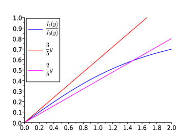
Figure 10: Ratio of the Bessel functions and the curves $\frac{y}{\beta J}$ for $\beta J=\frac{5}{3}<2$ and $\beta J=\frac{5}{2}>2$

For $\,h=+0$,  these equations are solved by $\,x_{1}=0=x_{2}\,$ but the corresponding stationary solution of the nonlinear Fokker-Planck equation becomes unstable for $\,\beta J>2\,$ where another stable solution with $\,x_{1}>0\,$ and $\,x_{2}=0$ (accompanied by the one reflected in the $\,x_{2}=0\,$ axes corresponding to $\,h=-0$)  appears by a supercritical pitchfork bifurcation, see FIG. 9.  For $\,h\not=0\,$ there is a single solution of Eqs. (4.108) with $\,{\rm sgn}(h)\,x_{1}>0\,$ and $\,x_{2}=0$.  These solutions describe the $2^{\rm nd}$ order phase transition in the $\,N\to\infty\,$ limit of the Gibbs state (4.101) for $\,h=0\,$ from the disordered stationary phase with $\,\mathbb{E}\,\vec{\sigma}_{n}=0\,$ for $\,\beta J\leq 2\,$ to the mixture of ordered ones with $\,\mathbb{E}\,\vec{\sigma}_{n}\not=0\,$ for $\,\beta J>2\,$ SFN (72). A pure ordered state is selected by turning on an infinitesimal magnetic field $\,h=+0\,$ and the other pure states are obtained by a simultaneous rotation of all spins.  The sharp transition disappears for (non-infinitesimal) $\,h\not=0$.

For $\,F>0\,$ and $\,h=+0$, there is no stable stationary solution for $\beta J>2$ but a stable periodic solution of the nonlinear Fokker-Planck equation

$$\rho(t,\theta)=\rho_{F=0}(\theta-MFt)\,,$$ (4.109)

where $\,\rho_{F=0}\,$ is the stable solution for $\,F=0$,  appears by a Hopf bifurcation: the phase transition becomes dynamical. This type of transition persists for $\,h>0\,$ sufficiently small and some intermediate $\,\beta$,  with a stable stationary solution occurring for smaller $\,\beta\,$ and stable periodic solution for higher $\,\beta$.  If we increase $\,h\,$ then the stable periodic solution turns back to a stable stationary solution for a sufficiently high $\,h$.  The corresponding phase diagram obtained by numerical simulations in refs. SK (86) and SSK (88) is sketched in FIG. 10.

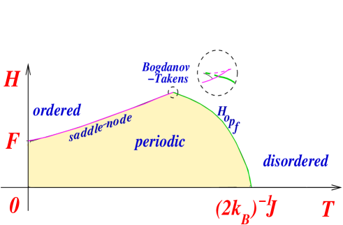
Figure 11: Phase diagram of the active rotator model of SK (86); SSK (88)

Note the presence of a $2^{nd}$ order transition corresponding to a saddle-node bifurcation, to which the analysis of Sec. IV.8 applies directly, as well as of the one corresponding to the Hopf bifurcation, with the crossing of the two involving a more complicated small transition region with a Bogdanov-Takens bifurcation SSK (88). More results on the large-deviations for empirical density and empirical current in the active rotators model, a prototypical example of a nonequilibrium system with mean-field interactions, will be described in ref. BGN .

Acknowledgements.  The author thanks the Mathematics Department of Helsinki University, and, in particular, Prof. A. Kupiainen, for the invitation to give a series of lectures on fluctuation relations and for the hospitality during author’s stay in Helsinki. The final work on these notes was done during author’s visit to KITPC in Beijing in July 2013. Support of the ANR project ANR-11-BS01-015-02 “STOSYMAP” is also acknowledged.

References

- BK (77) G. N. Bochkov, Yu. E. Kuzovlev: On general theory of thermal fluctuations in nonlinear systems. Sov.Phys. JETP 45 (1977), 125-130 Zh. Eksp. Teor. Fiz. 72 (1977), 238-
- BK (79) G. N. Bochkov, Yu. E. Kuzovlev: Fluctuation-dissipation relations for nonequilibrium processes in open systems. Sov.Phys. JETP 49 (1979), 543- Zh. Eksp. Teor. Fiz. 76 (1979), 1071-
- BK (81) G. N. Bochkov, Yu. E. Kuzovlev: Non-linear fluctuation-dissipation relations and stochastic models in nonequilibrium thermodynamics. I and II. Physica A 106 (1981), 443-479 and 480-520
- ECM (93) D. J. Evans, E. G. D. Cohen, G. P. Morriss: Probability of second law violations in shearing steady states. Phys. Rev. Lett. 71 (1993), 2401-2404 and 3616
- ES (94) D. J. Evans, D. J. Searles: Equlibrium microstates which generate the second law violating steady states. Phys. Rev. E 50 (1994), 1645
- (6) G. Gallavotti, E. D. G. Cohen: Dynamical ensembles in non-equilibrium statistical mechanics. Phys. Rev. Lett. 74 (1995), 2694-2697
- (7) G. Gallavotti, E. D. G. Cohen: Dynamical ensembles in stationary states. J. Stat. Phys. 80 (1995), 931-970
- (8) C. Jarzynski: A nonequilibrium equality for free energy differences. Phys. Rev. Lett. 78 (1997), 2690-2693
- J (07) C. Jarzynski: Comparison of far-from-equilibrium work relations, C. R. Physique 8 (2007), 495-506
- (10) C. Jarzynski: Equilibrium free energy differences from nonequilibrium measurements: a master equation approach. Phys. Rev. E 56 (1997), 5018
- K (98) J. Kurchan: Fluctuation theorem for stochastic dynamics. J. Phys. A 31 (1998), 3719-3729
- LS (99) J. Lebowitz, H. Spohn: A Gallavotti-Cohen type symmetry in the large deviation functional for stochastic dynamics. J. Stat. Phys. 95 (1999), 333
- ES (02) D. J. Evans, D. J. Searles: The fluctuation theorem. Adv. in Phys., 51 (2002), 1529-1585
- G (08) G. Gallavotti: Fluctuation Theorem and chaos, European Physical Journal B 64 (2008), 315-320
- J (11) C. Jarzynski: Equalities and inequalities: irreversibility and the Second Law of Thermodynamics at the nanoscale, Annu. Rev. Condens. Matter Phys. 2 (2011), 329-251
- M (03) C. Maes: On the origin and the use of fluctuation relations for the entropy, Séminaire Poincaré 2 (2003), 29-62
- SF (12) R. E. Spinney, I. J. Ford: Fluctuation relations: a pedagogical overview, arXiv:1201.6381 [cond-mat.stat-mech]
- M (99) C. Maes: The Fluctuation Theorem as a Gibbs Property, J. Stat. Phys. 95 (1999), 367-392
- HS (01) T. Hatano, S. Sasa: Steady-state thermodynamics of Langevin systems. Phys. Rev. Lett. 86 (2001), 3463-3466
- C (99) Crooks, G. E.: The entropy production fluctuation theorem and the nonequilibrium work relation for free energy differences. Phys. Rev. E 60 (1999), 2721-2726
- R (06) F. Ritort: Single-molecule experiments in biological physics: methods and applications, J. Phys. C (Cond. Mat.) 18 (2006), R531-R583
- CG (08) R. Chetrite, K. Gawȩdzki: Fluctuation relations for diffusion processes, Commun. Math. Phys. 282 (2008), 469-518
- (23) J.-P. Eckmann, C.-A. Pillet, L. Rey-Bellet: Non-equilibrium statistical mechanics of anharmonic chains coupled to two heat baths at different temperatures. Comm. Math. Phys. 201 (1999), 657-697
- (24) J.-P. Eckmann, C.-A. Pillet, L. Rey-Bellet: Entropy production in nonlinear, thermally driven hamiltonian systems, J. Stat. Phys. 95 (1999), 305-331
- S (12) U. Seifert: Stochastic thermodynamics, fluctuation theorems, and molecular machines, Rep. Prog. Phys. 75 (2012), 126001
- S (05) U. Seifert: Entropy production along a stochastic trajectory and an integral fluctuation theorem, Phys. Rev. Lett. 95 (2005), 040602(1-4)
- L (61) R. Landauer: Irreversibility and heat generation in the computing process, IBM Journal of Res. and Dev., 5:3 (1961), 183-191
- B (82) Ch. H. Bennett: The Thermodynamics of Computation - a review, Int. J. Theor. Phys. 21 (1982), 905-940
- A (11) B. Andresen: Current Trends in Finite-Time Thermodynamics, Angew. Chem. Int. Ed. 50 (2011), 2690-2704
- AMM (11) E. Aurell, C. Mejía-Monasterio, P. Muratore-Ginanneschi: Optimal protocols and optimal transport in stochastic thermodynamics, Phys. Rev. Lett. 106 (2011), 250601(1-4)
- AGM (12) E. Aurell, K. Gawȩdzki, C. Mejía-Monasterio, R. Mohayaee, P. Muratore-Ginanneschi: Refined Second Law of Thermodynamics for fast random processes, J. Stat. Phys. 147 (2012), 487-505
- N (67) E. Nelson: Dynamic Theories of Brownian Motion, Princeton University Press, Princeton N.J. 1967
- BB (97) J.-D. Benamou, Y. Brenier: A numerical method for the optimal time-continuous mass transport problem and related problems, in Monge Ampère Equation: Applications to Geometry and Optimization. (Deerfield Beach, FL, 1997), Amer. Math. Soc., Providence R.I. 1999, pp. 1-11
- BB (99) J.-D. Benamou, Y. Brenier: A computational fluid mechanics solution to the Monge-Kantorovich mass transfer problem, Numer. Math. 84 (1999), 375-393
- V (03) C. Villani: Topics in Optimal Transportation, Graduate Studies in Mathematics Vol. 38, American Mathematical Society, Providence R.I. 2003
- V (04) C. Villani: Optimal Transport: Old and New, Grundlehren der mathematischen Wissenschaften Vol. 338, Springer Berlin, 2008
- S (11) http://www.rdmag.com/news/2011/07/magnetic-memory-and-logic-could-achieve-ultimate-energy-efficiency
- JKO (98) R. Jordan, D. Kinderlehrer, F. Otto: The variational formulation of the Fokker Planck equation, SIAM J. Math. Anal. 29 (1998), 1-17
- B (12) A. Bérut, A. Arakelyan, A. Petrosyan, S. Ciliberto, R. Dillenschneider, E. Lutz: Experimental verification of Landauer’s principle linking information and thermodynamics, Nature 483 (2012), 187-189
- SS (07) T. Schmiedl, U. Seifert: Optimal finite-time processes in stochastic thermodynamics, Phys. Rev. Lett. 98 (2007), 108301(1-4)
- BF (03) Y. Brenier, U. Frisch, M. Hénon, G. Loeper, S. Matarrese, R. Mohayaee, A. Sobolevski: Reconstruction of the early Universe as a convex optimization problem, Mon. Not. R. Astron. Soc. 346 (2003), 501-524
- GSS (08) A. Gomez-Marin, T. Schmiedl, U. Seifert: Optimal protocols for minimal work processes in underdamped stochastic thermodynamics, J. Chem. Phys. 129 (2008), 024114(1-8)
- EK (10) M. Esposito, R. Kawai, K. Lindenberg, C. Van den Broeck: Efficiency at maximal power of low-dissipation Carnot engines, Phys. Rev. Lett. 105 (2010), 150603(1-4)
- AMM (12) E. Aurell, C. Mejía-Monasterio, P. Muratore-Ginanneschi: Boundary layers in stochastic thermodynamics, Phys. Rev. E 85 (2012), 020103(R)(1-4)
- MMP (12) P. Muratore-Ginanneschi, C. Mejía-Monasterio, L. Peliti: Heat release by controlled continuous-time Markov jump processes, arXiv:1203.4062v1 [cond-mat.stat-mech]
- MG (12) P. Muratore-Ginanneschi: On the use of stochastic differential geometry for non-equilibrium thermodynamics modeling and control, arXiv:1210.1133 [cond-mat.stat-mech]
- H (80) P. Hänggi: Connection between deterministic and stochastic descriptions of nonlinear systems, Helv. Phys. Acta 53 (1980), 491-496
- SSD (82) J. M. Sancho, M. San Miguel, D. Dürr, Adiabatic elimination for systems of Brownian particles with non-constant damping coefficients, J. Stat. Phys. 28 (1982), 291-305 Sancho-San Miguel-Duerr, J. Stat. Phys. 28, 291 (1982)
- CBE (12) A. Celani, S. Bo, R. Eichhorn, E. Aurell: Anomalous thermodynamics at the micro-scale, arXiv:1206.1742 [cond-mat.stat-mech]
- H (78) P. Hänggi: Stochastic processes II: Response theory and fluctuation theorems, Helv. Phys. Acta 51 (1978), 202–219
- PJP (09) J. Prost, J.-F. Joanny, J. M. R. Parrondo: Generalized fluctuation-dissipation theorem for steady-state systems, Phys. Rev. Lett. 103 (2009), 090601(1-4)
- (52) R. Chetrite, S. Gupta: Two refreshing views of fluctuation theorems through kinematics elements and exponential martingale, J. Stat. Phys. 143 (2011), 543-584
- CKP (94) L.F. Cugliandolo, J. Kurchan, G. Parisi: Off equilibrium dynamics and aging in unfrustrated systems J. Physique I 4 (1994), 1641-1656
- LCZ (05) E. Lippiello, F. Corberi, M. Zannetti: Off-equilibrium generalization of the fluctuation dissipation theorem for Ising spins and measurement of the linear response function, Phys. Rev. E 71, (2005), 036104(1-9)
- BMW (09) M. Baiesi, C. Maes, B. Wynants: Nonequilibrium linear response for Markov dynamics, I: jump processes and overdamped diffusions, J. Stat. Phys. 137 (2009), 1094- 1116
- CFG (08) R. Chetrite, G. Falkovich, K. Gawȩdzki: Fluctuation relations in simple examples of non-equilibrium steady states, J. Stat. Mech. (2008) P08005
- K (57) R. Kubo: Statistical-mechanical theory of irreversible processes. I. General theory and simple applications to magnetic and conduction problems, J. Phys. Soc. Japan 12 (1957), 570-586
- C (11) L. F. Cugliandolo: The effective temperature, arXiv:1104.4901 [cond-mat.stat-mech]
- CG (09) R. Chetrite, K. Gawȩdzki: Eulerian and Lagrangian pictures of non-equilibrium diffusions, J. Stat. Phys. 137 (2009), 890-916
- SS (06) T. Speck, U. Seifert: Restoring a fluctuation-dissipation theorem in a nonequilibrium steady state, Europhys. Lett. 74 (2006), 391-396
- GPC (09) J. R. Gomez-Solano, A. Petrosyan, S. Ciliberto, R. Chetrite, K. Gawȩdzki: Experimental verification of a modified fluctuation-dissipation relation for a micron-sized particle in a non-equilibrium steady state, Phys. Rev. Lett. 103 (2009), 040601
- GPC (11) J. R. Gomez-Solano, A. Petrosyan, S. Ciliberto, C. Maes: Fluctuations and response in a non-equilibrium micron-sized system, J. Stat. Mech. (2011), P01008
- G (54) M. S. Green: Markoff random processes and the statistical mechanics of time-dependent phenomena. II. Irreversible processes in fluids, J. Chem. Phys 22 (1954), 398-413
- BLR (00) F. Bonetto, J. L. Lebowitz, L. Rey-Bellet: Fourier law, achallenge to theorists, in: Mathematical Physics 2000, eds. Fokas, A., Grigoryan, A., Kibble, T., Zegarlinski, B., Imperial College Press, London 2000, pp. 128-150
- BK (07) Bricmont, J., Kupiainen, A.: Fourier’s Law from Closure Equations, Phys. Rev. Lett. 98 (2007), 214301
- FW (84) M. I. Freidlin, A. D. Wentzell: Random Perturbations of Dynamical Systems. Springer, New York, 1984
- DV (75) M. D. Donsker, S. R. S. Varadhan: Asymptotic evaluation of certain Markov process expectations for large time. part I, Commun. Pure Appl. Math. 28 (1975), 1-47; part II, 28 (1975), 279-301; part III, 29 (1976), 389-461; part IV, 36 (1983), 183-212
- DS (89) J. D. Deuschel, D. W. Stroock: Large Deviations. Academic Press, Boston, 1989
- DZ (98) A. Dembo, O. Zeitouni: Large Deviations Techniques and Applications, 2nd ed. Springer, New York, 1998
- CCM (07) V. Y. Chernyak, M. Chertkov, S. V. Malinin, R. Teodorescu: Non-equilibrium thermodynamics for functionals of current and density, arXiv:0712.3542 [cond-mat.stat-mech], unpublished
- MNW (08) C. Maes, K. Netocny, B. Wynants: Steady state statistics of driven diffusions, Physica A 387 (2008), 2675-2689
- T (11) H. Touchette: A basic introduction to large deviations: Theory, applications, simulations, in R. Leidl and A. K. Hartmann (eds), Modern Computational Science 11: Lecture Notes from the 3rd International Oldenburg Summer School, BIS-Verlag der Carl von Ossietzky Universität, Oldenburg 2011
- E (06) W. E, E. Vanden-Eijnden: Towards a theory of transition paths, J. Stat. Phys. 123 (2006), 503-523
- CCM (09) V. Chernyak, M. Chertkov, S. Malinin, R. Teodorescu: Non-Equilibrium thermodynamics and topology of currents, J. Stat. Phys. 137 (2009), 109-147
- RT (02) L. Rey-Bellet, L. E. Thomas: Fluctuations of the entropy production in anharmonic chains, Ann. Henri Poinc. 3 (2002), 483-502
- (76) F. Bouchet, K. Gawȩdzki, C. Nardini: Macroscopic fluctuations theory around difusions with mean-field coupling, in preparation
- BDG (06) L. Bertini, A. De Sole, D. Gabrielli, G. Jona-Lasinio, C. Landim: Large deviation approach to non equilibrium processes in stochastic lattice gases, Bull. Braz. Math. Soc., New Series 37 (2006), 611-643
- DG (87) D. A. Dawson, J. Gärtner: Large deviations from the McKean-Vlasov limit for weakly interacting diffusions, Stochastics 20 (1987), 247-308
- BDG (05) L. Bertini, A. De Sole, D. Gabrielli, G. Jona-Lasinio, C. Landim: Current fluctuations in stochastic lattice gases, Phys. Rev. Lett. 94 (2005), 020601
- BD (05) T. Bodineau, B. Derrida: Distribution of current in nonequilibrium dif- fusive systems and phase transitions, Phys. Rev. E 72 (2005), 066110
- BDL (08) T. Bodineau, B. Derrida, V. Lecomte, F. van Wijland: Long range correlations and phase transition in non-equilibrium diffusive systems, J. Stat. Phys. 133 (2008), 1013-1031
- SFN (72) H. Silver, N. E. Frankel, B. W. Ninham: A class of mean field models, J. Math. Phys. 13 (1972), 468–474
- SK (86) S. Shinomoto, Y. Kuramoto: Phase transitions in active rotator systems, Prog. Theor. Phys. 75 (1986), 1105-1110
- K (75) Y. Kuramoto: Self-entrainment of a population of coupled nonlinear oscillators, in International Symposium on Mathematical Problems in Theoretical Physics, ed. H. Araki, Lecture Notes in Physics 30, Springer, New York 1975, pp. 420-422
- GPP (12) G. Giacomin, K. Pakdaman, X. Pellegrin, Ch. Poquet: Transitions in active rotator systems: invariant hyperbolic manifold approach, SIAM J. Math. Analysis 44 (2012), 4165-4194
- M (05) M. C. Marchetti: Depinning and plasticity of driven disordered lattices, in: Proceedings the XIX Sitges Conference on Jamming, Yielding, and Irreversible Deformations in Condensed Matter, Sitges, Barcelona, Spain 2004, arXiv:cond-mat/0503660 [cond-mat.soft]
- SSK (88) H. Sakaguchi, S. Shinomoto, Y. Kuramoto: Phase transitions and their bifurcation analysis in a large population of active rotators with mean-field coupling, Prog. Theor. Phys. 79 (1988), 600-607