The metal-insulator transition in disordered solids: How theoretical prejudices influence its characterization A critical review of analyses of experimental data

Abstract

In a recent experimental study, Siegrist et al. [Nature Materials 10, 202–208 (2011)] investigated the metal-insulator transition (MIT) induced by annealing in GeSb₂Te₄ and related phase-change materials. The authors concluded that these materials exhibit a discontinuous MIT with a finite minimum metallic conductivity, and that they violate the Mott criterion for the critical charge carrier concentration. The striking contrast between their work and reports on many other disordered substances from the last 35 years motivates the present in-depth study of the influence of the MIT criterion used on the character of the MIT derived.

First, we discuss in detail the inherent biases of various approaches to locating the MIT, that is to discriminating between just metallic samples and weakly insulating ones which exhibit hopping conduction with very low characteristic temperatures. Second, reanalyzing the GeSb₂Te₄ data, we show that this material resembles other disordered solids to a large extent: According to a widely-used approach, the temperature dependences of the conductivity, $\sigma(T)$, of GeSb₂Te₄ may likewise be interpreted in terms of a continuous MIT. Careful checking the justification of the corresponding fits, however, uncovers discrepancies which currently render an unambiguous interpretation impossible. Moreover, we give several arguments against the violation of the Mott criterion stated by Siegrist et al.; it is traced back to the authors’ inappropriate considering shallow instead of deep impurity states. Third, examining previous experimental studies of crystalline Si:As, Si:P, Si:B, Ge:Ga, CdSe:In, Cd_0.95Mn_0.05Se, Cd_0.95Mn_0.05Te_0.97Se_0.03:In, disordered Gd, and nanogranular Pt-C, we show that substantial problems in the interpretation of $\sigma(T)$ can also be detected in numerous studies which claim the MIT to be continuous: Evaluating the logarithmic derivative $\mbox{d}\ln\sigma/\mbox{d}\ln T$ highlights serious inconsistencies. In part, they are common to all such studies and seem to be generic, in part, they vary from experiment to experiment. Fourth, for four qualitatively different phenomenological models of the temperature and control parameter dependence of the conductivity, we present the respective flow diagrams of this logarithmic derivative. In consequence, the likely generic inconsistencies seem to originate from the MITs being discontinuous and occurring when $\mbox{d}\sigma/\mbox{d}T=0$ at infinitely small $T$, in contradiction to most of the original interpretations. The experiment-dependent inconsistencies, however, cannot be understood in this way; they may arise from measurement problems.

Because of the large number and diversity of the experiments considered, the inconsistencies uncovered in this review provide overwhelming evidence against the common, localization theory motivated interpretations, which are based on the assumption that $\sigma(T)\propto T^{p}$ with $p=1/2$ or $1/3$ at the MIT. Thus, the question about the character of the MIT in disordered solids has to be considered as still open. The primary challenges now lie in improving the measurement precision and accuracy, rather than in extending the temperature range, and in developing a microscopic theory which explains the seemingly generic features of $\mbox{d}\ln\sigma/\mbox{d}\ln T$.

Keywords: metal-insulator transitions, doped crystalline semiconductors, amorphous semiconductors, nucleation and growth

1 Introduction

For more than fifty years, localization in disordered systems, in particular the corresponding metal-insulator transition (MIT), has attracted a lot of interest from both theoreticians and experimentalists.Lag.etal.09 ; Abr.10 ; Mott.90 ; Mott.Davi ; Lee.Rama ; Beli.Kirk ; Edw.95 ; Edw.etal.95 ; L98 ; Moe.Adk ; Ever.Mirl Milestones on this way have been Anderson noting the absence of diffusion in certain lattices with disorder,Ande.58 Mott’s concept of the minimum metallic conductivity,Mott.72 the scaling theory of localization,Abra.etal and the renormalization group approach incorporating electron-electron interaction into localization theory.Fink.83a Experimentally, localization in three-dimensional systems has been studied in a large number of disordered solids, such as heavily doped crystalline semiconductors (in which the disorder arises from the randomly positioned impurities), amorphous transition-metal semiconductor alloys, granular metals, and nanocrystalline substances.Edw.95 ; Edw.etal.95 ; L98 ; Moe.Adk Many of these solids are or may become application relevant; therefore they are often considered to be among the materials.Mott.Davi In various experiments, the MIT has been triggered by diverse control parameters: composition / doping, stress, magnetic field, light, as well as structure, see, for example, Refs. Yama.etal.67, ; Zabr.Zino, ; Shaf.etal.89, ; Her.etal.83, ; Moe.etal.83, ; Moe.etal.99, ; Tho.etal.83, ; Waf.etal.99, ; Bis.etal.83, ; vMo.etal.83, ; Wojt.etal.86, ; Dietl.etal.86, ; Katsu.87, ; Glod.etal.93, ; Lei.etal.98, ; Sie.etal.11, ; Mis.etal.11, ; Giv.Ova.12, ; in part, these publications substantially contradict each other.

The MIT in disordered solids is primarily a zero-temperature phenomenon. – We do not consider here the case of an MIT which is interrelated with a structural or magnetic phase transition. Such transitions usually occur at some finite (i.e., nonzero) temperature, for example in VO₂ and V₂O₃.Mott.Zina By means of doping or applying pressure, the critical temperature may be reduced to zero.McW.etal.73 – Therefore, in the field of localization, a sample is said to be metallic if its dc conductivity, $\sigma$, is expected to tend to some finite value as the temperature, $T$, goes to zero, and it is called insulating if $\sigma$ is expected to tend to zero as $T\rightarrow 0$. Of course, for the insulating samples, $\sigma$ is finite at any finite $T$ due to thermally activated non-metallic transport, in particular variable-range hopping.cla

Hence, in studying the MIT, each evaluation of experimental data includes some $T\rightarrow 0$ extrapolation: Early work on two- and three-dimensional systems judged the $\sigma(T)$ curves from a rather global perspective. Only samples for which $\sigma$ drops exponentially with decreasing $T$ were classified as insulating, while all other samples were regarded as metallic.Mott.72a ; Adk.78 Later, for three-dimensional systems, when more dense sets of control parameter values were considered, the focus concentrated on $\sigma(T\rightarrow 0)$ extrapolations of low-temperature data from the control parameter region thought of as metallic.Lee.Rama These analyses are based on microscopic theories yielding augmented power laws, $\sigma=a+b\,T^{p}$, as derived in Refs. Alt.Aro.79, and News.Pepp, . In this approach, samples with positive extrapolated $\sigma(T=0)$ value are regarded as metallic, while all other samples are classified as insulating.

Simultaneously with this change in the data analysis approach, the majority opinion on the character of the MIT in three-dimensional samples turned: It shifted from initially supporting Mott’s idea of a discontinuous transition with a finite minimum metallic conductivity toward favoring a continuous transition in accord with the scaling theory of localization.Lee.Rama Nowadays, most of the experts in this field seem to be certain about the continuity of the MIT, see, for example, Ref. HvL.11, . Nevertheless, two repeatedly observed phenomena are in conflict with the continuity hypothesis: the scaling of the $T$ dependences of $\sigma$ in the hopping regionMoe.85 ; Sara.Dai.02 and the existence of specific low-temperature minima in the $T$ dependences of the logarithmic $T$ derivative of $\sigma$, $\mbox{d}\ln\sigma/\mbox{d}\ln T$.Moe.Adk ; Moe.etal.99 – Because of the focus on properties of individual samples, we here mostly use total derivative symbols although $\sigma$ depends not only on $T$ but also on a control parameter. –

The concurrence of the changes in the data analysis approach and in the majority opinion on the character of the MIT provokes a naive question: May it be that this opinion change was caused merely by the difference between the biases inherent to the analysis approaches rather than by improvements in the experiments?

To support our question, we recall the following: In the literature, two different MIT criteria have been used in confirming the scaling theory of localization for the three-dimensional case and in disproving it for the two-dimensional case, respectively. In the former situation, the augmented power law extrapolation criterion has been applied to determine the critical value of the control parameter.Lee.Rama ; HvL.11 In contrast, in the latter case, the sign change of the derivative, $\mbox{d}\sigma/\mbox{d}T$, at the lowest measuring temperature has been considered as indicator of the change in the nature of conduction.Krav.etal.94 ; Krav.Sara One exception within the studies of two-dimensional systems acts as additional motivation for our question: Reference Feng.etal.01, used the $T\rightarrow 0$ extrapolation ansatz $\sigma=a+b\,T^{2}$ and obtained an empirical model of a continuous MIT.

At this point, the reader is invited to scroll down for a moment to take a brief look at Figures 3, 4, 8, 9, 10, 16, 17, and 19, which regard various disordered solids: All these diagrams contrast $T$ dependences of $\mbox{d}\ln\sigma/\mbox{d}\ln T$ obtained by direct numerical differentiation of experimental data with dashed-dotted curves derived from augmented power laws, $\sigma=a+b\,T^{p}$. The slopes of the former and of the latter relations differ qualitatively from each other, again and again! This observation, together with the historical remarks above, will surely awaken or strengthen the reader’s interest in a detailed analysis of the $T\rightarrow 0$ extrapolation problem, which is central to this review.

Further motivation for our above question about the role of the interpretation bias comes from a recent investigation of the MIT in specific three-dimensional disordered systems. The report by Siegrist et al. on GeSb₂Te₄ and similar phase-change materialsSie.etal.11 claims to obtain surprising results: Annealing amorphous films of such substances induces a crystallization process with increasing temperature whereby a nanocrystalline structure is formed.Sie.etal.11 During this transformation, $\sigma$ increases by orders of magnitude while $\sigma(T)$ changes qualitatively, which indicates an MIT.Sie.etal.11 Classifying the samples according to the sign of $\mbox{d}\rho/\mbox{d}T$ at the measuring temperature, Siegrist et al. conclude that the studied phase-change materials exhibit a finite minimum metallic conductivity, in contrast to various other disordered substances. Moreover, the authors state that the phase-change materials violate the Mott criterion for the critical charge carrier concentration. They interpret these features as originating from an “unparalleled quantum state of matter” resulting from “pronounced disorder but weak electron correlation”,Sie.etal.11 see also Ref. Sch.11, .

Remarkably, the work by Siegrist et al.Sie.etal.11 differs from previous publications which claim continuity of the MIT not only concerning the substance investigated but also with respect to the data evaluation approach used. This again raises the question about the influence of the choice of the data analysis method on the character of the MIT obtained.

Therefore, we here scrutinize the justification of the conclusions of Ref. Sie.etal.11, , reanalyzing data from this work. Due to the interpretation uncertainties mentioned above, we take a neutral, phenomenological perspective and avoid, as far as possible, any bias caused by focusing on a particular microscopic theory. Our present study shows that the $\sigma(T)$ for GeSb₂Te₄ resemble results from previous studies on disordered solids to a large extent. A part of the data can be well approximated by the ansatz $\sigma=a+b\,T^{1/2}$, so that, in the same way as in other investigations, the MIT could be characterized as continuous. However, when checking the justification of this approach by studying the behavior of $\mbox{d}\ln\sigma/\mbox{d}\ln T$, new insight is gained: Both the sample classifications according to the sign of $\mbox{d}\rho/\mbox{d}T$, on the one hand, and according to the fit of the augmented power law $\sigma=a+b\,T^{1/2}$ to the measured data, on the other hand, are called into question.

The situation gets even more complicated when data from a subsequent GeSb₂Te₄ study, Ref. Vol.etal.15, , by three of the authors of Ref. Sie.etal.11, are additionally taken into account: Therein, the $T$ range was extended by one order of magnitude, and continuity of the MIT was concluded from augmented power law approximations of the measured $\sigma(T)$. However, as will be shown in our analysis of the $T$ dependences of $\mbox{d}\ln\sigma/\mbox{d}\ln T$, also these augmented power law approximations substantially fail close to the MIT.

The observations described in the previous two paragraphs suggest to take a broader view. Thus, in the following, we here examine various publications on the MIT in other solids, Refs. Shaf.etal.89, ; Stu.etal.93, ; Ros.etal.80, ; Ros.etal.83, ; Tho.etal.83, ; Waf.etal.99, ; Sara.Dai.02, ; Dai.etal.91, ; Wata.etal.98, ; Wojt.etal.86, ; Dietl.etal.86, ; Glod.etal.93, ; Mis.etal.11, ; Sac.etal.11, , from the same perspective. In doing so, one is confronted with similar problems as for GeSb₂Te₄: In numerous cases, the behavior of $\mbox{d}\ln\sigma/\mbox{d}\ln T$ obtained numerically from the measurements without making any assumptions is not consistent with the common interpretation in terms of a continuous MIT with, on the metallic side, $\sigma(T)$ following $\sigma=a+b\,T^{p}$ where $p=1/2$ or $1/3$. More precisely, for many samples which are classified as metallic in the publications cited above, $\mbox{d}\ln\sigma/\mbox{d}\ln T$ in fact increases with decreasing $T$ over a wide $T$ range, whereas a decrease is expected according to the ansatz $\sigma(T)=a+b\,T^{p}$.

One result of this examination is particularly striking: For various solids, there are even allegedly metallic samples for which the $T$ dependence of $\mbox{d}\ln\sigma/\mbox{d}\ln T$ has negative slope in spite of $\sigma(T)$ decreasing so slowly with $T$ that $\mbox{d}\ln\sigma/\mbox{d}\ln T\ll 1/3$. – Remarkably, below about 2 K, also one of the CdSe:In samples from Refs. Zha.etal.90, ; Aha.etal.92, ; Zha.Sara.95, shows exactly this correlation, although it is claimed to exhibit hopping conduction in those publications. –

These findings provide valuable information about the character of the MIT: First, the disproofs of the finite minimum metallic conductivity hypothesis in the analyzed publications, which are based on augmented power law fits with $p=1/2$ or $1/3$, cannot be considered conclusive. Second, the here observed correlation between value and sign of the slope of $\mbox{d}\ln\sigma/\mbox{d}\ln T(T)$ indicates that, in the limit $T\rightarrow 0$, the control parameter dependence of $\sigma$ is very likely discontinuous at the MIT. – We substantiate this implication by comparing flow diagrams of $\mbox{d}\ln\sigma/\mbox{d}\ln T(T)$ obtained from four qualitatively different phenomenological models in a separate section of the present review. –

In several cases, however, the $T$ dependence of $\mbox{d}\ln\sigma/\mbox{d}\ln T$ exhibits a maximum which is incompatible with the seemingly generic behavior of this quantity, as it has been described and interpreted in the previous three paragraphs. Since these maxima are experiment-specific, further, very careful investigations of the same $T$ range are needed. In this way, we identify key points for the design of future related experiments.

The present review is organized as follows: Section 2 discusses various approaches to the precise determination of the transition point between metallic and insulating phases, the first and most important difficulty of experiments on the MIT. – Readers in a hurry may focus on Subsections 2.2, 2.3, 2.4, and, in particular, 2.6. – Section 3 is devoted to GeSb₂Te₄: In its first part, Subsection 3.1, $\sigma(T)$ data from Refs. Sie.etal.11, and Vol.etal.15, are reanalyzed by means of alternative approaches. In doing so, we demonstrate inconsistencies in the data sets from Ref. Sie.etal.11, which render it impossible to reach definite conclusions about the nature of conduction for three of the samples. Moreover, we explain why a part of the sample classifications of Ref. Vol.etal.15, seems to be incorrect, so that the characterization of the MIT therein is called into question. In the second part of Section 3, Subsection 3.2, several arguments against the hypothetical violation of the Mott criterion by GeSb₂Te₄ are presented; this deviation is found to be not real but to result from an invalid assumption on the participating states. – Subsection 3.2 may be skipped on first reading. – Section 4 compares our findings on GeSb₂Te₄ with results of a multitude of studies on various other disordered solids. Here we show that, in numerous publications favoring continuity of the MIT, severe interpretation problems can be uncovered by taking the behavior of $\mbox{d}\ln\sigma/\mbox{d}\ln T$ into consideration. Section 5, evaluating simple phenomenological hypotheses, studies how the character of the MIT determines qualitative properties of sets of $T$ dependences of $\mbox{d}\ln\sigma/\mbox{d}\ln T$ for various control parameter values. It demonstrates that such flow diagrams obtained directly from experimental data can be an informative fingerprint of the character of the zero-temperature phenomenon MIT. Finally, Section 6 summarizes our results and draws conclusions for future studies.

In Appendix A, relations between the effective mass, permittivity, critical charge carrier concentration of the MIT, charge carrier concentration at which $\mbox{d}\sigma/\mbox{d}T$ changes sign in the low-$T$ limit, and corresponding $\sigma$ value are deduced by means of dimensional analyses. These results are robust with respect to a broad class of theoretical approximations, also regarding the incorporation of the electron-electron interaction. Appendix B is devoted to mathematical aspects in the interpretation of observations of scaling of $T$ dependences of $\sigma$, in particular to the hidden suppositions in this way of concluding the existence of a finite minimum metallic conductivity. Finally, to ensure that our data evaluations are easily reproducible, Appendix C explains the sophisticated numerical differentiation method for functions given by noisy values at non-equidistant points which is the basic tool for a large part of the reanalyses presented here.

2 Criteria for detecting the MIT

Although, at first glance, the identification of metallic and insulating phases of disordered solids seems to be a simple task, it is far from trivial.Ros.etal.94 ; Moe.etal.99 Therefore, the general aspects of various approaches, in particular their implicit preconditions and consequences, are discussed in detail in this section.

2.1 Sign change of $\mbox{d}\rho/\mbox{d}T$ at the measuring temperature

Siegrist et al.Sie.etal.11 describe the current state of the literature on three-dimensional systems as follows: In experimental studies, the sign of the temperature derivative of the resistivity, $\mbox{d}\rho/\mbox{d}T$, is taken as criterion, where positive and negative $\mbox{d}\rho/\mbox{d}T$ indicate metallic and insulating behavior, respectively.Sie.etal.11 Note that this classification refers to the current measuring temperature. – Alternatively, as done below, $\mbox{d}\sigma/\mbox{d}T$ can be considered which always has the opposite sign. – Furthermore, Siegrist et al. state that this approach by experimentalists contrasts with theoretical investigations.Sie.etal.11 Those studies consider transport as metallic if, as $T\rightarrow 0$, the conductivity $\sigma$ tends to a finite value, and as insulating if $\sigma$ vanishes.Sie.etal.11

That summary of the literature is incomplete: As already mentioned in Section 1 and discussed in more detail in Subsection 2.3 as well as Sections 3 and 4, also quite a number of experimental studies have focused on $\sigma(T\rightarrow 0)$ extrapolations based on microscopic theories for the metallic phase. They concern not only doped crystalline semiconductors but also amorphous transition metal semiconductor alloys and granular systems, see, for example, Refs. Tho.etal.83, , Sac.etal.11, , and Dod.etal.81, .

More importantly, the above usage of notions by Siegrist et al., which, by the way, seems to be rather popular among nonspecialists in localization still nowadays, is misleading: The transition from metallic to insulating behavior at $T=0$ and the sign change of $\mbox{d}\rho/\mbox{d}T$ at finite $T$ are two different, only loosely related phenomena. They should not be confused by using the same term “metal-insulator transition” for both of them. This is illustrated by qualitative considerations in the following three paragraphs.

Consider $\sigma$ as function of $T$ and some control parameter $x$. In the limit $T\rightarrow 0$, the conductivity is identical to zero in the insulating region. – From the empirical perspective, the existence of such a region is a hypothesis, although a very plausible one. Consider, for example, Figure 2 of Ref. Tho.etal.83, : The convergence of the finite $T$ curves to a sharp transition is not proven. In principle, $\lim_{T\rightarrow 0}\sigma(T,x)$ might also continuously vanish in some very rapid manner. – The onset of metallic conduction happens at the $x$ value where $\lim_{T\rightarrow 0}\sigma(T,x)$ suddenly starts to deviate from zero. There, this function of $x$ is not smooth but has some peculiarity. That means it is either discontinuous or at least not infinitely often differentiable. This non-analytic behavior of $\lim_{T\rightarrow 0}\sigma(T,x)$ indicates a phase transition, more precisely, a quantum phase transition.

On the contrary, the room-temperature resistivity, $\rho(T=293\ {\rm K},x)$, seems to be a smooth function of $x$ in the region of the sign change of $\mbox{d}\rho/\mbox{d}T(T=293\ {\rm K},x)$. To the best of our knowledge, no indication for any peculiarity (non-analyticity) of $\rho(T=293\ {\rm K},x)$ correlated with the sign change of $\mbox{d}\rho/\mbox{d}T(T=293\ {\rm K},x)$ has been reported up to now. Thus, the sign change of $\mbox{d}\rho/\mbox{d}T(T=293\ {\rm K},x)$ very likely does not arise from a phase transition.

Moreover, if there are two interfering mechanisms yielding additive $T$-dependent resistivity contributions, $\rho_{i}(T,x)$, with different signs of $\mbox{d}\rho_{i}/\mbox{d}T$ (as in the case of the Kondo effect), $\rho(T,x={\rm const.})$ may exhibit a maximum or minimum, as two curves in the shaded transition region in Figure 2 of Ref. Sie.etal.11, do. Although $\mbox{d}\rho/\mbox{d}T=0$ at such an extremum, this feature cannot be interpreted as transition between qualitatively different phases since $\rho(T,x={\rm const.})$ does not exhibit any non-analyticity there.

Nevertheless, one might expect the finite-$T$ criterion $\mbox{d}\rho/\mbox{d}T=0$ to yield approximate results for the critical value of the control parameter $x$ and possibly for the hypothetical minimum metallic conductivity and the hypothetical maximum metallic resistivity. To which extent does such an estimate depend on the measuring temperature? To answer this question, we now compare room-temperature data with measurements at temperatures of the order of 1 K for four groups of materials. Thereby, as working definition, we use the terms room-temperature minimum metallic conductivity, $\sigma_{\rm rtmm}$, and low-temperature minimum metallic conductivity, $\sigma_{\rm ltmm}$, to denote the $\sigma$ values which are related to $\mbox{d}\rho/\mbox{d}T=0$ in the respective temperature regions.

First, for GeSb₂Te₄, Ref. Sie.etal.11, obtains a maximum metallic resistivity of 2 to $3\ {\rm m\Omega cm}$ considering the temperature range from 5 to $290\ {\rm K}$. Compared to the logarithmic scale in Figure 3 of Ref. Sie.etal.11, , the uncertainty factor of 1.5 is rather small. The only sample with $\rho$ falling in this interval was prepared by annealing at $275\ {\rm{}^{o}C}$. Its $\rho(T)$ is almost constant over the whole temperature range considered; it varies far less than the respective $\rho(T)$ of the “neighboring” samples, which were annealed at 250 and $300\ {\rm{}^{o}C}$. Thus, the values of the critical annealing temperature and of the minimum metallic conductivity depend only slightly on the measuring temperature, so that in this case $\sigma_{\rm rtmm}\approx\sigma_{\rm ltmm}$.

Second, the Mooij rule,Moo.73 an empirical relation between the room-temperature values of $\mbox{d}\rho/\mbox{d}T$ and $\rho$, states: For a large number of disordered alloys, the sign of $\mbox{d}\rho/\mbox{d}T$ changes from plus to minus with increasing $\rho$ at about $150\pm 50\ {\rm\mu\Omega cm}$. Disordered solids with $\rho(300\ \mbox{K})\lesssim 1000\ {\rm\mu\Omega cm}$, however, do usually not exhibit any increase in $\rho(T)$ by several orders of magnitude with decreasing $T$, provided they do not undergo some phase transition at finite $T$. Accordingly, $\sigma_{\rm rtmm}>5\ \sigma_{\rm ltmm}$.

Third, consider the amorphous Si_1-xCr_x films from Refs. Moe.etal.83, and Moe.etal.85, , prepared by electron-beam evaporation. Their Cr contents cover the range from $x=0.09$ to 0.26. At low $T$, $\mbox{d}\sigma/\mbox{d}T$ changes sign when $x\approx 0.15$ and $\sigma\approx 270\ {\rm\Omega^{-1}cm^{-1}}$, see Figures 3 and 5 of Ref. Moe.etal.83, and Figure 7 of Ref. Moe.etal.85, . At room-temperature, however, up to $x=0.26$, where $\sigma=1360\ {\rm\Omega^{-1}cm^{-1}}$, all samples exhibit positive $\mbox{d}\sigma/\mbox{d}T$, see Figures 1 and 7 of Ref. Moe.etal.85, . Thus, at room-temperature, they all are to be regarded as insulating according to the $\mbox{d}\rho/\mbox{d}T<0$ criterion. Therefore, when using only room-temperature data, one would overestimate the critical Cr content at least by a factor of 1.7, and $\sigma_{\rm rtmm}>5\ \sigma_{\rm ltmm}$.

Fourth, concerning localization, the best investigated material is heavily doped crystalline Si:P.L98 ; HvL.11 In the mK region, $\mbox{d}\sigma/\mbox{d}T$ changes sign at a P concentration of about $4\times 10^{18}\ {\rm cm^{-3}}$, when $\sigma\approx 60\ {\rm\Omega^{-1}cm^{-1}}$, see Figure 3 of Ref. Stu.etal.93, , compare Ref. Ros.etal.81, . At room-temperature, however, due to the electron-phonon scattering in the exhaustion region, $\mbox{d}\rho/\mbox{d}T$ stays positive within the very wide $\sigma$ range from $10^{-3}$ to $10^{3}\ {\rm\Omega^{-1}cm^{-1}}$, except for a small interval around $10^{2}\ {\rm\Omega^{-1}cm^{-1}}$, see Figure 1 of the NIST study Ref. Bul.etal.68, . (Si:P does not comply with Mooij’s rule.) This $\sigma$ range is related to a P concentration range from roughly $10^{13}$ to about $10^{20}\ {\rm cm^{-3}}$, see Figure 4 of Ref. Thu.etal.80, . Hence, for room-temperature, inferring the character of conduction from the sign of $\mbox{d}\rho/\mbox{d}T$ fails dramatically: Samples are marked as metallic even if the P concentration is smaller by a factor of $10^{5}$ than the critical concentration obtained from low-temperature measurements. Furthermore, in contrast to the above considered materials, $\sigma_{\rm rtmm}<2\times 10^{-5}\ \sigma_{\rm ltmm}$ for the region of low P concentrations.

In summary, the classification of the conduction character according to the sign of $\mbox{d}\rho/\mbox{d}T$ at an arbitrarily chosen measuring temperature is usually highly questionable. The reason is the absence of any non-analyticity in the control parameter dependence of the conductivity at such hypothetical MIT points. Moreover, this criterion suffers from considerable uncertainties. In particular, when it is applied to room-temperature data, both, false-metallic and false-insulating classifications in comparison to corresponding low-temperature evaluations are not unlikely.

2.2 Sign change of $\mbox{d}\rho/\mbox{d}T$ in the limit as $T\rightarrow 0$

In the previous subsection, we demonstrated that the identification of the nature of conduction according to the sign of $\mbox{d}\rho/\mbox{d}T$ at some arbitrary measuring temperature leads to severe problems. Nevertheless, the question arises whether or not such a differential approach may indicate the MIT at least in the limit as $T\rightarrow 0$. In order to apply this criterion, one would have to determine the control parameter value for which $\mbox{d}\rho/\mbox{d}T=0$ at various temperatures. Its $T\rightarrow 0$ limit would identify the MIT.

In practice, in particular for two-dimensional systems, the focus is on the transport at the lowest experimentally accessible temperature, $T_{\rm lea}$, often in the mK range.Krav.etal.94 ; Krav.Sara That means, the sign change of $\mbox{d}\rho/\mbox{d}T(T_{\rm lea},x)$ is regarded as the indication of the MIT, instead of a corresponding $T\rightarrow 0$ extrapolation. Of course, this approach can be meaningful only if $|\mbox{d}^{2}\rho/\mbox{d}T^{2}|$ is so small at this hypothetical MIT that the influence of $T_{\rm lea}$ on its location is negligible. Fortunately, this condition seems to be often fulfilled; the width of the corresponding $x$ range, however, decreases with $T$.

Nevertheless, one should be very cautious since the issue is far more profound than it appears at first glance: Using this criterion means to favor a particular character of the MIT, namely discontinuity, and thus the existence of a finite minimum metallic conductivity. Our statement can be substantiated in two ways: It results from a short mathematical consideration, and from purely experimental experience.

First, we take the mathematical perspective. Suppose the properties of the investigated material can be continuously modified where the extent of the modification is measured by a real control parameter $x$ with $x\in[x_{\rm a},x_{\rm b}]$.

Focusing now on the $T$ region $(0,T_{\rm lea}]$, we consider $\sigma(T,x)$ and $\mbox{d}\rho/\mbox{d}T(T,x)$ to be continuous functions of $T$ and $x$ where $\sigma(T,x)>0$. Without loss of generality, we suppose that, when $T={\rm const.}\in(0,T_{\rm lea}]$, both these functions increase strictly monotonically with $x$. Suppose, furthermore, that $\mbox{d}\rho/\mbox{d}T(T_{\rm lea},x_{\rm a})<0$ and that $\mbox{d}\rho/\mbox{d}T(T_{\rm lea},x_{\rm b})>0$. Then, $\mbox{d}\rho/\mbox{d}T(T_{\rm lea},x)$ changes sign at some critical control parameter value, $x_{\rm c}\in(x_{\rm a},x_{\rm b})$, and $\sigma_{\rm c}=\sigma(T_{\rm lea},x_{\rm c})>0$.

In practically applying the hypothetical MIT criterion considered in this subsection, as pointed to above, we suppose that (i) $\mbox{d}\rho/\mbox{d}T(T,x_{\rm c})=0$ for any $T\in(0,T_{\rm lea}]$, and hypothesize that (ii) $x_{\rm c}$ marks the MIT.

From (i) and the suppositions above, we deduce that, in case $x<x_{\rm c}$ and $T\in(0,T_{\rm lea}]$, $\mbox{d}\rho/\mbox{d}T(T,x)<0$ holds, so that $\mbox{d}\sigma/\mbox{d}T(T,x)>0$. Thus $\sigma(T,x)\leq\sigma(T_{\rm lea},x)<\sigma_{\rm c}$ and, therefore, $\lim_{T\rightarrow 0}{\sigma(T,x)}<\sigma_{\rm c}$. Finally, due to (ii), we even expect that, for $x<x_{\rm c}$, $\lim_{T\rightarrow 0}{\sigma(T,x)=0}$. – Such a limiting behavior may result when, on the insulating side of the MIT, the rapid decrease of $\sigma(T,x={\rm const.})$ sets in at the lower temperature the closer $x$ to $x_{\rm c}$, see Subsections 2.4 and 2.5. – For $x\geq x_{\rm c}$ and $T\in(0,T_{\rm lea}]$, we obtain $\sigma(T,x)\geq\sigma(T_{\rm lea},x)\geq\sigma_{\rm c}$ in an analogous way, so that $\lim_{T\rightarrow 0}{\sigma(T,x)}\geq\sigma_{\rm c}$ in this $x$ region.

Therefore, under the above physically plausible suppositions, the hypothetical MIT criterion considered here implies that $\lim_{T\rightarrow 0}{\sigma(T,x)}$ is discontinuous at $x_{\rm c}$ – the limit jumps there from 0 to $\sigma_{\rm c}$ – and that $\sigma_{\rm c}$ has the meaning of a finite minimum metallic conductivity. Thus, in the present situation, already by the choice of the MIT criterion, one determines which character of the MIT one will infer from the experimental data.

Now, we consider the experimental experience: For many three-dimensional systems, the $\sigma$ value which corresponds to $\mbox{d}\rho/\mbox{d}T$ changing sign at low $T$ was found to roughly agree with Mott’s minimum metallic conductivity estimate,Mott.Davi ; Mott.72 ; Mott.82

$$\sigma_{\rm M}=C\frac{e^{2}}{\hbar d_{\rm c}}\,.$$ (1)

Here $d_{\rm c}$ denotes the interatomic distance of the transport enabling constituents at the MIT (e.g., P atoms in crystalline Si:P) and $C$ a numerical constant of order 0.025 to 0.05;$d_{\rm c}=n_{\rm c}^{\ -1/3}$, where $n_{\rm c}$ is the corresponding critical density. For example, Ganguly et al. explicitly used this sign change criterion to determine the value of $\sigma_{\rm M}$ for oxide systems, see Ref. Gan.etal.84, . Further support for this correlation comes from the original references of the data compiled in Figure 10 of Ref. Mott.Kaveh, ; moreover, concerning crystalline Si:P and amorphous Si_1-xCr_x, see Figure 3 of Ref. Stu.etal.93, and Figure 7 of Ref. Moe.etal.85, , respectively. Thus, in the literature, using the criterion $\mbox{d}\rho/\mbox{d}T=0$ at $T_{\rm lea}$ for defining the MIT usually results in support for Mott’s idea of the finite minimum metallic conductivity.

It has to be stressed, however, that the frequently observed correlation between the features $\mbox{d}\rho/\mbox{d}T=0$ and $\sigma=\sigma_{\rm M}$ concerns only measurements at $T_{\rm lea}$. Without a further assumption, it does neither identify the MIT nor does it imply that Mott’s reasoning is correct. In particular, this correlation alone does not justify the conclusion that, for each sample with negative $\mbox{d}\rho/\mbox{d}T(T_{\rm lea},x)$, the conductivity $\sigma(T)$ cannot saturate at some nonzero value (far) below $\sigma_{\rm M}$ as $T\rightarrow 0$. In other words, this experimental experience is not sufficient to exclude that there might be metallic samples with negative $\mbox{d}\rho/\mbox{d}T(T_{\rm lea},x)$. Hence, interpreting solely the correlation between the $T_{\rm lea}$-related features $\mbox{d}\rho/\mbox{d}T=0$ and $\sigma=\sigma_{\rm M}$ as evidence for Mott’s minimum metallic conductivity theory overvalues the experimental findings.

In this sense, relying only on the MIT criterion $\mbox{d}\rho/\mbox{d}T=0$ in the limit as $T\rightarrow 0$ means to bias the data analysis, and to presume the existence of a finite minimum metallic conductivity. That is why the corresponding conclusion by Siegrist et al.Sie.etal.11 is not surprising. It is the natural consequence of these authors focusing on the sign change of $\mbox{d}\rho/\mbox{d}T$.

Note, furthermore, that the MIT criterion $\mbox{d}\rho/\mbox{d}T=0$ in the limit as $T\rightarrow 0$ does not seem to be in accord with any of the currently available microscopic theories: First, because of the following argument, this criterion is incompatible with the interpretation in terms of an Anderson transition caused by the mobility edge crossing the Fermi energy. According to this model, just at the MIT, the number of electrons (or holes) excited to extended states would be proportional to $T$. It is hard to believe that these electrons do not cause a corresponding increase in $\sigma$ with rising $T$.Moe.etal.83 – Thus, the derivation of Eq. (1) as zero-temperature evaluation of the Kubo-Greenwood formula by Mott in Ref. Mott.72, is not consistent with his interpretation of experimental data in terms of the activation energy of hopping tending to zero as $x\rightarrow x_{\rm c}$ in the same work. – Our incompatibility argument, however, does not disprove the hypothetical MIT criterion considered here because the interpretation in terms of an Anderson transition is based on a strong simplification; it neglects the electron-electron interaction. Second, to the best of our knowledge, also the currently available microscopic theories incorporating electron-electron interaction cannot provide a justification for this criterion. The reason is that none of them yields its logical consequence, that is a discontinuous MIT with a finite minimum metallic conductivity.

Now, if the sign change of $\mbox{d}\rho/\mbox{d}T$ in the limit as $T\rightarrow 0$ did not arise from the MIT, how could it be understood? An alternative explanation was provided by an analysis of the influence of the electron-electron interaction: According to Altshuler and Aronov, the electron-electron interaction should yield a $T^{1/2}$ contribution to $\sigma(T)$.Alt.Aro.79 Rosenbaum et al. pointed out that its sign should be determined by the relative importance of exchange and Hartree terms, which in turn is controlled by the ratio of screening length and Fermi wave length.Ros.etal.81 ; Lee.Rama Therefore, the variation of the screening length may cause two sign changes of the $T^{1/2}$ contribution.Ros.etal.81 This interpretation has been very influential up to now.

Nevertheless, in our opinion, the applicability of this theoretical idea by Rosenbaum et al.Ros.etal.81 is highly questionable: The point is that the value of the exponent, $1/2$, seems to disagree with the experimental findings. For samples which exhibit negative $\mbox{d}\rho/\mbox{d}T$ at $T_{\rm lea}$ and which were classified as metallic in the respective original publications, a series of such discrepancies is presented in our Section 4.

Concerning samples with positive $\mbox{d}\rho/\mbox{d}T$ at $T_{\rm lea}$, being very likely metallic, doubts about the exponent value $1/2$ arise from three publications: Already Figure 1 of Ref. Ros.etal.81, shows that, for crystalline Si:P, the exponent $1/3$ enables a clearly better approximation of the experimental data than $1/2$. The Figures 3a and 3b of Ref. Dai.etal.92, testify that, for crystalline Si:B, $\sigma$ versus $T^{1/2}$ plots exhibit substantial curvature in the low-$T$ range. – The authors of Ref. Dai.etal.92, model this feature by additionally taking into account a localization contribution to $\sigma(T)$, but the deviation visible in Figure 3b questions the physical meaning of such fits. – These observations are consistent with a study of amorphous Si_1-xCr_x in which a power law contribution to $\sigma(T)$ with the exponent $0.19\pm 0.03$ was identified by collective augmented power law fits to sets of conductivity differences of pairs out of 15 samples.Moe.90a Remarkably, the corresponding decomposition of $\sigma(T)$ ceases to be applicable when, with decreasing $x$, $\mbox{d}\rho/\mbox{d}T$ at $T_{\rm lea}$ changes sign from plus to minus.Moe.90a

Furthermore, in a very recent theoretical investigation, Di Sante et al. studied the interplay of thermal lattice deformations and static disorder in the vicinity of the MIT.Di_Sante.etal Claiming continuity of the transition, they state the existence of a control parameter interval within which $\mbox{d}\rho/\mbox{d}T$ is negative although $\sigma$ tends to finite values when $T\rightarrow 0$, and denote it as region of “bad insulators”. – The choice of this name is not in accord with the definition of an insulator as we use it here. – The authors conclude that, in this control parameter range, transport is governed by the strong $T$ dependence of the density of states, rather than by the $T$ dependence of the scattering of the electrons.Di_Sante.etal However, Di Sante et al. focus on the situation of a half-filled band, and it seems at least questionable whether their conclusions remain valid for arbitrary band filling. Moreover, the quantitative comparison of this theory to experiment is hindered by the following: Reference Di_Sante.etal, does not report any specific exponent value for the power law governing $\sigma(T)$ at the MIT.

According to the above three paragraphs, the theoretical interpretations of the sign change of $\mbox{d}\rho/\mbox{d}T$ given in Ref. Ros.etal.81, and Di_Sante.etal, should be considered with great caution, so that alternative hypotheses have to checked too. Therefore, at the current stage, it seems quite possible that the criterion $\mbox{d}\rho/\mbox{d}T=0$ in the limit as $T\rightarrow 0$ may indeed identify the MIT.

Due to the described unclear situation, the development of a more appropriate theory is required. Fortunately, one of its features can be easily predicted because, for dimensional reasons, Eq. (1) is robust, also with respect to the incorporation of electron-electron interactions: If a theory yields a relation which links the distance $d_{\rm c}$ with any characteristic conductivity value, and if electron charge, Planck constant, effective mass, and permittivity are the only dimensioned parameters of this theory, then the so obtained relation must be universal and have the form of Eq. (1); for the proof see Appendix A. Independently of the character of the MIT, the condition $\mbox{d}\rho/\mbox{d}T=0$ in the limit as $T\rightarrow 0$ is a natural way to define such a characteristic conductivity value. In case a finite minimum metallic conductivity exists, it should equal a universal multiple of this characteristic conductivity value; it might even coincide with this value.

We now continue with our phenomenological analysis: Currently, to the best of our knowledge, the MIT criterion $\mbox{d}\rho/\mbox{d}T=0$ in the limit as $T\rightarrow 0$ is only a hypothesis. How could it be justified? It seems natural to regard all samples with $\mbox{d}\rho/\mbox{d}T>0$ at $T_{\rm lea}$ as metallic. However, for the inverse approach, the classification of all samples with $\mbox{d}\rho/\mbox{d}T<0$ at $T_{\rm lea}$ as insulating, further arguments and / or additional measurements are required. In particular, this concerns the $\rho(T)$ curves with small negative slope, for which the interpretation in terms of activated transport may seem counterintuitive.

Nevertheless, one can easily imagine a situation where such samples are indeed insulating. Let us assume that some kind of hopping is the only relevant conduction mechanism and that, as already surmised by Mott,Mott.72 its mean activation energy tends continuously to 0 as the MIT is approached. In this case, the existence of insulating samples with quite flat, nonexponential $\rho(T)$ is not counterintuitive but natural: All the samples close to the MIT for which the characteristic temperature, corresponding to the mean hopping energy, is smaller than the lowest measuring temperature should behave this way, see also Subsections 2.4 and 2.5.

Thus, also the identification of insulating samples in the penultimate paragraph according to the sign of $\mbox{d}\rho/\mbox{d}T$ for $T\rightarrow 0$ may be correct. To find out whether or not it is correct indeed, we have to ask: Which value does the mean hopping energy tend to as the MIT is approached? Empirical support for the hypothesis that the mean hopping energy continuously approaches zero comes from scaling of the $\sigma(T,x={\rm const.})$ curves for various values of $x$ on the insulating side of the MIT, see Subsection 2.5.

In conclusion, the unclear situation described above poses the challenge to find out which of the samples with nonexponential $\rho(T)$ and $\mbox{d}\rho/\mbox{d}T<0$ at $T_{\rm lea}$ are metallic and which are insulating. Various approaches to this question will be discussed in the following subsections.

2.3 Breakdown of the augmented power law approximation

An alternative to considering $\mbox{d}\rho/\mbox{d}T$ at $T_{\rm lea}$ is to detect the MIT by quantitatively analyzing measurements in some low-temperature range in terms of a microscopic theory: Starting from a theory-based ansatz for $\sigma(T)$ with adjustable parameters, one determines the value of the control parameter at which this equation ceases to be valid. Ideally, such an analysis should be performed for both sides of the MIT. In this subsection, we focus on the metallic side. For the corresponding consideration of the non-metallic region see Subsection 2.4.

Considering metallic conduction, augmented power laws,

$$\sigma(T,x)=a(x)+b(x)\,T^{p}\,,$$ (2)

were derived for different situations. Altshuler and Aronov studied the superposition of electron-electron interaction and static disorder and obtained $p=1/2$, see Ref. Alt.Aro.79, . They derived, however, Eq. (2) from a perturbation theory, so that its applicability very close to the MIT is at least questionable. Nevertheless, in various low-$T$ experiments, Eq. (2) has been claimed to describe measured data rather well, see, for example, Refs. Zabr.Zino, and Tho.etal.83, .

Newson and Pepper additionally incorporated the $T$ dependence of the diffusion constant into the result by Altshuler and Aronov; for this they used the Einstein relation linking conductivity and diffusion constant.News.Pepp Their approach again results in Eq. (2), but with a smaller exponent: Now $p=1/3$, see Ref. News.Pepp, and compare Ref. Mali.etal, . The derivation, however, presumes $a\ll b\,T^{1/3}$. In several cases, this version of Eq. (2) was claimed to be more appropriate for describing the experimental data than Eq. (2) with $p=1/2$, see Refs. Waf.etal.99, , Giv.Ova.12, , and Mali.etal, .

In practice, the choice of the value of $p$ seems not to influence the conclusion about the qualitative character of $\lim_{T\rightarrow 0}\sigma(T,x)$ in the vicinity of the MIT.Stu.etal.93 Nevertheless, a modification of $p$ as well as a variation of the $T$ range taken into account in the fit usually cause a small shift of the resulting MIT point; an example will be given in Subsection 4.2.

In a few studies, extensions of Eq. (2) were used to model the experimental data. For example, investigating crystalline Si:(P,B), Hirsch et al. included a second $T$-dependent term accounting for a weak-localization correction due to inelastic electron-electron collisions,

$$\sigma(T,x)=a(x)+b(x)\,T^{p}+c(x)\,T^{q}$$ (3)

with $q=3/4$, see Ref. Hir.etal.88, . Not surprisingly, including such a second $T$-dependent term improves the fit quality even if the model is not physically justified;Hir.etal.88 ; Moe.89 ; Hir.etal.89 see also Subsection 2.6.

In all data analyses based on Eq. (2) or (3), the diagnosis of the breakdown of the theoretical description is the crucial point. There are the following two approaches to this problem; both have to be combined to ensure that the sample classification is as reliable as possible.

First, relying on the validity of the considered ansatz, one determines the value of the control parameter at which one of the adjustable parameters ceases to have a physically reasonable value. In the present situation, one asks at which value of $x$ the parameter $a$ reaches 0.

Second, one checks for systematic deviations of the adjusted theoretical $\sigma(T)$ relation from the experimental data. This, however, is a fuzzy condition: The precision and accuracy of the experimental data as well as the width of the considered $T$ interval have great influence on strength and assessment of deviations. Presumably because of these uncertainties, the search for systematic deviations has played only a minor role in the literature. Thus, essential information was often lost; we will demonstrate this in Sections 3 and 4.

It is important to note that, when using solely the first approach, one demands only one of two necessary conditions for the validity of Eq. (2) to be satisfied. Thus, in such an analysis, there is a considerable risk that some insulating samples very close to the MIT are misinterpreted as metallic. Therefore, since the function $\sigma(T={\rm const.},x)$ seems to be continuous at the MIT for any $T>0$, it is not unlikely that one only gets out what is put into the model used in the data analysis, that is the continuity of $\lim_{T\rightarrow 0}\sigma(T,x)$. For this reason, analyses based solely on augmented power law fits without careful applicability checks exhibit a substantial bias in favor of a continuous MIT.

The way out of this dilemma is to consider another observable additionally to $\sigma(T)$. To that end, however, it is not necessary to measure a further transport coefficient or some thermodynamic observable. Already considering a specific derivative of $\sigma(T)$ can be very helpful as will be explained in Subsections 2.6 and 2.8. The situation concerning the incorporation of alternative observables will be discussed in Subsection 2.7.

2.4 Breakdown of the stretched Arrhenius law approximation

We now turn to the insulating side of the MIT. There, at low $T$, the transport proceeds by some kind of hopping conduction. Such mechanisms cause $\sigma(T,x={\rm const.})$ to follow a stretched Arrhenius law,

$$\sigma(T,x)=\sigma_{0}(x)\,\exp(-(T_{0}(x)/T)^{\nu})\,.$$ (4)

The characteristic temperature $T_{0}$ depends on the distance to the MIT; it seems to vanish as the MIT is approached,Mott.72 see also Subsection 2.2. The exponent $\nu$ is mechanism-dependent: Thermal excitation over some finite gap implies $\nu=1$. In case of variable-range hopping without Coulomb interaction, $\nu$ equals 1/3 and $1/4$ for two- and three-dimensional systems, respectively,Mott.69 compare, for example, Figure 8s in the Supplementary Information of Ref. Sie.etal.11, . If, however, Coulomb interaction has to be taken into account in variable-range hopping, $\nu=1/2$ is expected for two-dimensional as well as for three-dimensional samples,Efro.Shkl see also Refs. Zabr.Zino, and Moe.etal.85, .

The prefactor $\sigma_{0}$ may be weakly $T$-dependent, which is neglected in our Eq. (4). A reliable determination of $\nu$ is therefore only possible if the $\sigma$ values cover a very wide range, ideally several orders of magnitude.

It seems natural to classify all those samples as insulating for which $\sigma(T)$ approximately obeys Eq. (4). – In doing so, one implicitly assumes this relation to be valid down to $T=0$. – However, simply regarding all other samples as metallic is not justified for the following two reasons.

First, there is no sharp distinction between exponential and nonexponential $\sigma(T)$: For example, assume the ratio $\sigma(6\,{\rm K})/\sigma(4.2\,{\rm K})$ amounts to 256, 16, 4, 2, 1.4, 1.2, 1.1, 1.05, 1.02, or 1.01. At which value could metallic behavior set in?

Second, in its pure form, an exponential law such as Eq. (4) is usually only an approximation valid for $T\ll T_{0}$. However, as already pointed to in Subsection 2.2, $T_{0}(x)$ seems to vanish continuously as the MIT is approached. This limiting behavior, which is very likely but not completely certain, has an important consequence: Consider $\sigma(T,x={\rm const.})$ measurements by means of some cryostat down to its lowest experimentally accessible temperature, $T_{\rm lea}$. Then, for any value of $T_{\rm lea}$, there is a finite interval of $x$ adjacent to the MIT within which $T_{0}(x)$ is smaller than $T_{\rm lea}$. Thus, for all samples belonging to this interval of $x$, it is impossible to observe an exponential decrease in $\sigma(T)$ by orders of magnitude using the specific cryostat although these samples are insulating. Compare Figure 1 of Ref. Moe.etal.99, and the explanation in its caption.

Note that the second argument holds regardless of the experimental technique used, for studies down to 4.2 K as well as for measurements in a dilution refrigerator. With respect to the continuous variation of the control parameter $x$, one can even state: Since the $T$ scale is set by $T_{0}(x)$, it is very likely impossible to stay at low temperatures while passing the MIT.

Because of this problem, and due to the possible weak $T$ dependence of $\sigma_{0}$, fits based on Eq. (4) do not allow the reliable identification of insulating samples very close to the MIT. Therefore, these samples may easily be misinterpreted as metallic in a corresponding analysis. In evaluating experimental data, one is quite often confronted with such interpretation ambiguities since the critical exponent of the characteristic temperature, $T_{0}(x)$, seems to be rather large: In studies of crystalline n-Ge:(As,Ga) and amorphous Si_1-xCr_x, in which, at low $T$, the $\sigma(T,x={\rm const.})$ could be well approximated by Eq. (4) with $\nu=1/2$, critical exponent values of $2.1\pm 0.1$ and $3.0\pm 0.4$, respectively, were obtained.Zabr.Zino ; Moe.90b

Note, moreover, that an unambiguous classification of metallic and insulating samples based solely on describing $\sigma(T)$ alternatively by Eqs. (2) or (4) is in principle impossible if $\sigma(T)$ is proportional to $T^{p}$ at the MIT: The two analytic functions modeling $\sigma(T)$ on both sides of the MIT do not fit together at the critical value of $x$, in contradiction to the experimental experience that $\sigma(T={\rm const.},x)$ seems to be continuous for any $T>0$.

2.5 Breakdown of scaling of $T$ dependences of $\sigma$

In several studies of two- and three-dimensional systems,Zabr.Zino ; Moe.etal.83 ; Moe.85 ; Sara.Dai.02 ; Moe.etal.85 ; Liu.etal.92 ; Krav.etal.95 but by far not in all such investigations, the identification of insulating samples has been facilitated by empirical scaling of $\sigma(T,x={\rm const.})$ curves,

$$\sigma(T,x)=\sigma_{\rm scal}(T/T_{0}(x))\,.$$ (5)

Here, $T_{0}(x)$ denotes an $x$-dependent characteristic temperature; $T_{0}(x)>0$. This equation links measurements on different samples. In particular, it relates samples with quite flat $\sigma(T)$ to samples with exponential $\sigma(T)$. We remark that, for three-dimensional systems, the scaling relation Eq. (5) is incompatible with basic ideas of the scaling theory of localization, despite the similarity of the terms used.Moe.86

The important point is that, provided Eq. (5) remains valid when $T\rightarrow 0$, $\lim_{T\rightarrow 0}\sigma(T,x)$ is independent of $x$. Thus, in all the samples for which the $\sigma(T,x={\rm const.})$ data sets are linked to each other by this relation, the nature of electrical conduction must be the same. We stress that this statement does not rely on specific assumptions of any particular microscopic theory, in contrast to the analysis methods discussed in Subsections 2.3 and 2.4.

Deep in the non-metallic region where $\sigma$ follows a stretched exponential $T$ dependence according to Eq. (4), scaling is reflected by the prefactor $\sigma_{0}(x)$ being a constant independent of $x$. For $\nu=1/2$, such a behavior has been observed quite often.Zabr.Zino ; Moe.etal.83 ; Moe.85 ; Sara.Dai.02 ; Moe.etal.85 This exponential limit of Eq. (5) has a twofold relevance: It indicates that all the samples with $\sigma(T,x)$ satisfying Eq. (5) belong to the insulating phase. Furthermore, it enables to define an absolute scale of $T_{0}$.

Therefore, when the MIT is approached from the insulating side, the breakdown of the validity of Eq. (5) very likely indicates the transition; for a detailed reasoning see Appendix B. This criterion has a great advantage over the approaches discussed in the previous subsections: In a scaling analysis, the reduced temperature, $T/T_{0}$, may vary over several orders of magnitude, compare Fig. 4 in Ref. Moe.etal.83, and Fig. 2 in Ref. Liu.etal.92, . Thus, the reliability of $\sigma(T\rightarrow 0)$ extrapolations and the trustworthiness of sample classifications close to the MIT can be considerably improved by utilizing the scaling relation Eq. (5).

Note, however, that there are essential preconditions for Eq. (5) being possibly valid. First, it can only hold if all but one conduction mechanisms are frozen out. Therefore, its applicability is always limited by some material-dependent upper temperature threshold, $T_{\rm utt}$, the value of which is determined by the maximum tolerable contribution of the second most relevant mechanism to $\sigma(T)$.Moe.etal.85 – In the case of amorphous Si_1-xCr_x, it amounts to roughly 50 K;Moe.etal.85 for doped crystalline semiconductors, it is far smaller and may even fall below 1 K, compare Subsection 4.5. – Second, Eq. (5) can only be valid over a wide range of the reduced temperature $T/T_{0}$ if there is merely a single transport-relevant length scale, that means, if the disordered solid considered is sufficiently homogeneous. To ensure this, the influences of macroscopic and mesoscopic inhomogeneities have to be effectively suppressed. Here, we remind that such a scaling of $\sigma(T,x={\rm const.})$ curves seems to be destroyed by clustering.Moe.85 ; Moe.etal.85

In its general form, the scaling relation Eq. (5) to hold can be concluded from experimental data for a set of $k$ samples either by a master curve constructionMoe.etal.83 ; Liu.etal.92 ; Krav.etal.95 or by checking whether or not $\mbox{d}\ln\sigma/\mbox{d}\ln T$ is a function of $\sigma$ alone.Moe.etal.85 The former approach requires adjusting the quotients of the $T_{0}$ values for $(k-1)$ pairs of samples by means of rescaling $T$, while the latter procedure is parameter-free. The degree to which Eq. (5) can be experimentally verified depends not only on the set of control parameter values considered as well as on precision and accuracy of resistance, temperature, and geometry measurements, but also on how well the preconditions specified in the previous paragraph are fulfilled.

The scaling of $\sigma(T,x={\rm const.})$ curves according to Eq. (5) has been interpreted as indication of the existence of a finite minimum metallic conductivity, $\sigma_{\rm mm}$, that means of the MIT being discontinuous.Moe.etal.83 ; Zha.Sara.95 ; Moe.85 ; Moe.etal.85 ; Krav.etal.95 This conclusion, however, is based on several more or less hidden assumptions. In order to identify them, we illuminate the details of this scaling analysis by means of a short mathematical consideration in Appendix B. There, we show that, under quite natural suppositions, the scaling of the $T$ dependences of $\sigma$ for several values of $x$ implies $T_{0}(x)\rightarrow 0$ as $x$ tends to the MIT value $x_{\rm c}$ and, moreover, that the limit $\lim_{t\rightarrow\infty}\sigma_{\rm scal}(t)$ coincides with the minimum metallic conductivity $\sigma_{\rm mm}$.

Furthermore, Appendix B explains why, because of the finiteness of $\sigma_{\rm mm}$, the $\sigma(T,x={\rm const.})$ must become more and more flat when the MIT is approached, in accord with the MIT criterion “Sign change of $\mbox{d}\rho/\mbox{d}T$ in the limit as $T\rightarrow 0$” considered in Subsection 2.2. This feature of $\sigma(T,x)$, however, has an unpleasant consequence: There is always some close vicinity of the MIT where it is impossible to prove scaling by constructing a mastercurve $\sigma_{\rm scal}(T/T_{0}(x))$ out of overlapping pieces.

As a side remark, we mention here that the observation of scaling according to Eq. (5) together with the plausible suppositions made in Appendix B imply a surprising conclusion: At any fixed $T\in(0,T_{\rm utt}]$, when varying $x$, one should cross a sharp boundary, located at $x_{\rm c}$, between non-metallic and metallic conduction. In other words, the zero-temperature phenomenon MIT – a discontinuous quantum phase transition – should be the endpoint of a line of continuous phase transitions in the finite-$T$ part of the $(x,T)$-plane. Therefore, $\sigma(T={\rm const.},x)$ should exhibit a non-analyticity at $x_{\rm c}$; see Section 4 of Ref. Moe.85, , in particular Figure 9 therein, and the introduction of Ref. Moe.08, . In consequence, $\partial\sigma/\partial T(T={\rm const.},x)$, too, should have a non-analyticity at the MIT, just where it changes sign.

In the case of amorphous Si_1-xCr_x, this hypothesis of a line of continuous phase transitions is supported by two observations: (i) The optimal exponent of a power law contribution to $\sigma(T,x)$ changes qualitatively just when $\mbox{d}\sigma/\mbox{d}T=0$, see Ref. Moe.90a, . (ii) The relation between two coefficients of a phenomenological model of $\sigma(T,x)$ for the metallic side seems to exhibit a non-analyticity coinciding with $\mbox{d}\sigma/\mbox{d}T=0$, see Refs. Moe.etal.85, and Moe.90b, .

The direct identification of such a composition tuned phase transition in $\sigma(T={\rm const.},x)$ would likely be hindered by the requirement of an extremely high degree of sample-to-sample reproducibility; presumably, $\Delta\sigma/\sigma$ would have to amount to one to a very few percent. However, if shallow impurity states play the dominant role, this problem can be circumvented by tuning the critical doping concentration by means of stress or magnetic field instead of tuning the doping concentration itself. In the two-dimensional case, this problem can be avoided by tuning the charge carrier concentration via a gate voltage; by reanalyzing such an experiment, first indications of the hypothesized peculiarity in $\sigma(T={\rm const.},x)$ separating regions of metallic and non-metallic conduction at finite $T$ were detected in Ref. Moe.08, . Moreover, focusing on correlations between $\sigma(T,x={\rm const.})$ and appropriate derivatives of this function or between $\sigma(T,x={\rm const.})$ and the exponent of an augmented power law approximation may help; compare Ref. Moe.90a, .

Nevertheless, in all these approaches, inhomogeneities can easily smooth out the hypothetical finite-$T$ phase transition. Paradoxically, their influence should be less disturbing when the measurements are performed at intermediate temperatures rather than at extremely low ones.Moe.08 The reason is that, in the insulating $x$ range, when $T<T_{\rm utt}$, the following holds for the immediate neighborhood of the MIT: The smaller $T$, the steeper is $\sigma(T={\rm const.},x)$, and the wider is the $\sigma$ range affected by a given, fixed uncertainty of $x$.

Finally, motivated by a dimensional consideration, we point to a possible universality of homogeneous disordered solids: Consider samples of two kinds of three-dimensional disordered solids. Suppose that the measured $\sigma(T,x)$ satisfy Eq. (5) with two separate $\sigma_{\rm scal}(t)$. Let us define both the respective scales of $T_{0}$ by means of Eq. (4). Then, although the minimum metallic conductivity value $\sigma_{\rm mm}=\lim_{t\rightarrow\infty}\sigma_{\rm scal}(t)$ is a material-dependent quantity, the ratio $\sigma_{\rm scal}(t)/\sigma_{\rm mm}$ should be a universal function of the reduced temperature $t=T/T_{0}$. This should hold not only when $\sigma_{\rm scal}$ depends on $t$ in an exponential manner, but also in the range of nonexponential behavior of $\sigma_{\rm scal}(t)$. Thus, the quotient of the characteristic conductivity values $\sigma_{0}$, defined by Eq. (4), and $\sigma_{\rm mm}$, corresponding to $\mbox{d}\sigma/\mbox{d}T=0$, should be material-independent, too; for amorphous Si_1-xCr_x, it amounts to $0.46\pm 0.14$, compare Refs. Moe.etal.83, and Moe.etal.85, .

2.6 Bounds obtained from the logarithmic derivative of $\sigma(T)$

Both the analyses of $\sigma(T)$ data based on Eqs. (2) and (4), which were discussed in Subsections 2.3 and 2.4, respectively, have an inherent disadvantage: They may misinterpret insulating samples very close to the MIT as metallic. The risk of such a misclassification can be largely reduced by additionally evaluating the logarithmic derivative,

$$w(T)=\frac{\mbox{d}\ln\sigma}{\mbox{d}\ln T}\,,$$ (6)

see Refs. Moe.etal.99, , Moe.89, , and Hir.etal.89, . Here, $\ln\sigma$ instead of $\sigma$ is considered in order to simplify the examination of an exponentially wide conductivity range. This quantity is differentiated with respect to $\ln T$ instead of with respect to $T$ to enable the clear discrimination between metallic and non-metallic $\sigma(T)$ which is explained in the following.

The logarithmic derivative $w(T)$ exhibits qualitatively different behavior for the augmented power law, Eq. (2) with $p>0$, and for the stretched Arrhenius relation, Eq. (4) with $\nu>0$. In the former case, that is for metallic samples,

$$w(T)=\frac{p\,b\,T^{p}}{a+b\,T^{p}}$$ (7)

holds, where $a+b\,T^{p}=\sigma(T)>0$ and $a=\sigma(0)>0$. In case the MIT is continuous, the logarithmic derivative stays constant at the MIT itself, $w(T)=p$ due to $a=0$.

Equation (7) looks simple but provides several experimentally checkable conclusions. Thus, for metallic samples, as $T$ vanishes, $w(T)$ becomes proportional to $T^{p}$ and tends to 0. If, moreover, $b>0$, then, as $T$ increases far beyond $(a/b)^{1/p}$, $w(T)$ approaches $p$. Therefore, plotting $w$ versus $T^{p}$ can test the validity of Eq. (2) over a wide $T$ range.

Furthermore, if measurements yield $w>0$ for a hypothetically metallic sample, then the parameter $b$ has to be positive as well. Hence, $0<w(T)<p$ must be fulfilled.

Even more important, for $w>0$ and thus $b>0$, the logarithmic derivative $w(T)$ always decreases with diminishing $T$. This is obvious from rewriting Eq. (7) as

$$w(T)=p\,\left(1-\frac{a}{a+b\,T^{p}}\right)\,.$$ (8)

In other words, for a sample with $w>0$ to be metallic, ${\mbox{d}}w/{\mbox{d}}T$ must be positive.

Consequently, if measurements yield simultaneously a positive value of $w$ and a negative value of ${\mbox{d}}w/{\mbox{d}}T$, then $\sigma(T)$ cannot be described by some augmented power law with a positive exponent. In this case, the sample considered is very likely not metallic but insulating. – Focusing on the slope of $w(T)$, we make use of a second derivative (in a generalized sense) of $\sigma(T)$ instead of a first derivative as it is considered in the ${\mbox{d}}\rho/{\mbox{d}}T=0$ criteria of the MIT discussed in Subsections 2.1 and 2.2. –

Assume now, $\sigma(T)$ follows the stretched Arrhenius relation Eq. (4) with positive $T_{0}$ and positive $\nu$, indicating that the considered sample is insulating. In this case, we obtain

$$w(T)=\nu\,(T_{0}/T)^{\nu}\,.$$ (9)

Thus, $w(T)$ is always positive. It increases with diminishing $T$, so that ${\mbox{d}}w/{\mbox{d}}T<0$, and it diverges as $T\rightarrow 0$.

It has to be stressed, however, that Eq. (9) can be expected to be a good quantitative description of experimental data only for the exponential limit. For this, $T$ has to be smaller than $T_{0}$, so that $w$ must exceed $\nu$.

Nevertheless, for any positive $w$, even if $w\ll\nu$, negative ${\mbox{d}}w/{\mbox{d}}T$ indicates non-metallic transport as, starting from Eq. (2), we concluded in the above considerations of $w(T)$ for the metallic side. Therefore, in this way, also a large part of the samples with quite flat $\sigma(T)$ can be unambiguously classified. – If $\sigma(T,x)$ obeys scaling according to Eq. (5), then ${\mbox{d}}w/{\mbox{d}}T$ should be negative even for any positive $w$;Moe.etal.85 compare Appendix B. –

In addition to its simplicity and unbiasedness for broad classes of conceivable $\sigma(T)$, the discrimination between metallic and insulating samples based on the sign of $\mbox{d}w/\mbox{d}T$ has still another big advantage: Graphs of $w(T)$ for sample sets close to the MIT contain direct, valuable information on the character of the MIT. This can be understood as follows.

Suppose the MIT is continuous and, on its metallic side, $\sigma(T,x)$ obeys Eq. (2) with some positive exponent $p$. Thus, $w(T)=p$ would hold at the MIT itself. Now, according to experimental experience, $w(T={\rm const.},x)$ always seems to decrease strictly monotonically when the MIT is approached from the insulating side and then crossed. Hence, as soon as the MIT has been crossed, that means as soon as $w<p$, $\mbox{d}w/\mbox{d}T$ should be positive. Therefore, for any supposed value of $p$, the existence of samples with simultaneously $0<w<p$ and $\mbox{d}w/\mbox{d}T<0$ is a strong argument against the hypothetical continuity of the MIT, that means against the continuity of $\lim_{T\rightarrow 0}\sigma(T,x)$.Moe.etal.99 ; Moe.Adk

The latter argument will play a central role in our reanalysis of numerous experimental studies of the MIT in Section 4. It will be supported by an exploration of possible structures of sets of $w(T)$ curves in Section 5. Therein, we compare four qualitatively different phenomenological models and exemplify how the character of the zero-temperature phenomenon MIT determines qualitative features of the separatrix between metallic and insulating $w(T)$ at finite $T$.

At this point, however, we have to emphasize a physical restriction on utilizing the simply structured Eqs. (7) and (9): They can only be valid if the temperature is so low that all but one conduction mechanisms are frozen out. There are many cases where this condition is not met. For example, in amorphous semiconductor transition-metal alloys, some high-temperature mechanism seems to considerably enhance the conductivity on both sides of the MIT above a threshold of the order of 50 K.Moe.etal.85 ; Moe.85 ; Moe.Adk It yields a positive contribution to $w(T)$ which increases with $T$. For insulating samples, its superposition with the hopping contribution, Eq. (9), causes $w(T)$ to exhibit a minimum; the corresponding $T$ value tends to 0 as the MIT is approached.Moe.etal.99 ; Moe.Adk Such a behavior of $w(T)$ is not restricted to amorphous solids, it can also be observed for nanocrystalline GeSb₂Te₄ above about 50 K, see Subsection 3.1, as well as for crystalline CdSe:In above about 2 K, see Subsection 4.5.

Over the last two and a half decades, evaluating the logarithmic derivative $w(T)$ for individual samples has proven to be very effective in checking the validity of the augmented power law, Eq. (2), as well as of its extended version, Eq. (3); see, for example, Refs. Moe.Adk, , Ros.etal.94, , Moe.89, , Hir.etal.89, , and YY.etal.11, . For this aim, the $w(T)$ data which are obtained by numerical differentiation directly from the measured $\sigma(T)$ are contrasted with the approximations of $w(T)$ resulting from analytic differentiation of Eqs. (2) or (3) with adjusted parameter values. This comparison highlights small but possibly qualitative deviations between experimental points and $\sigma(T)$ fits.Moe.89 ; Hir.etal.89 In particular, as pointed to above, for slowly varying $\sigma(T)$, the repeatedly observed increase in $w(T)$ with decreasing $T$ is not compatible with the metallic nature of transport; such samples should be insulating.Moe.89 ; Hir.etal.89 This data analysis approach will be basic to the reconsideration of a series of experimental key investigations of the MIT in various disordered solids in our Section 4.

In several cases, a second type of deviation between the $w(T)$ obtained by numerical differentiation and the corresponding analytical differentiation of the augmented power law, Eq. (2) fitted to $\sigma(T)$, has been observed: According to these $w$ versus $T^{p}$ plots, the numerically obtained $w(T)$ reaches 0 or rapidly tends to 0 already at some finite $T$ in disagreement with Eq. (7). Such a behavior may arise from a superposition of two mechanisms, see, for example, Figures 8 and 9 in Ref. Moe.etal.99, . Alternatively, the rapid decrease at finite $T$ may occur due to the measured $\sigma(T)$ data following an augmented power law with an exponent which is considerably larger than $p$; this seems to be the case in our Figure 8 below roughly 50 mK. Thermal decoupling of sample and thermometer is a possible reason for such behavior of $w(T)$. This explanation is particularly likely if, for different samples, the rapid decrease of $w(T)$ always sets in at roughly the same temperature. For example, Figure 1b of Ref. Sac.etal.11, seems to indicate a related problem; more such cases will be discussed in our Section 4.

Finally, we take up the universality hypothesis on the scaling of the $T$ dependences of $\sigma$ in different homogeneous disordered solids which was formulated in the last paragraph of the previous subsection. It implies that $w(T/T_{0})$ may be a material-independent function. In this case, for a series of insulating samples of different such solids, in the region of sufficiently low $T$, all the $w(T)$ curves together would form a common flow diagram without intersections. More specifically, for arbitrary two of these $w(T)$ curves, provided the respective codomains overlap each other, it would even be possible to collapse them by rescaling $T$ for one of the two samples by an appropriate factor.

2.7 Behavior of other observables near the MIT

In the preceding subsections, we discussed six MIT criteria which all focus on specific features of the temperature dependence of the conductivity (or resistivity). As we will see in Section 3 and 4, the respective classifications of samples into metallic and insulating ones often contradict each other. This begs the question of what additional information on the location of the MIT can be gained from studying other observables. At first glance, the idea of using such additional information to reach a less ambiguous classification may look promising. However, one has to be aware of two fundamental difficulties.

First, the MIT definition is based on the limit of $\sigma$ as $T\rightarrow 0$. – Furthermore, it presupposes that electric field strength and frequency are infinitely small and that the sample size is infinitely large; these three conditions are sufficiently well fulfilled in most experiments. – Likewise, when, instead of $\sigma$, another observable is considered, it is essential to determine its limiting value as $T\rightarrow 0$ for each sample; often, additionally, the limit concerning a further measurement parameter tending to zero has to be taken. These tasks may be very demanding, in particular in case the alternative observable diverges or tends from finite values to zero at one side of the MIT: One has to be aware that, in the non-metallic region, nonexponential and exponential $\sigma(T)$ may be correlated with qualitatively different $T$ dependences of the alternative observable.

Second, we will see in Sections 3 and 4 how reanalyses of $\sigma(T,x)$ data from various publications uncover systematic, apparently generic inconsistencies in the respective interpretations based on current localization theory. Thus, a sound and successful microscopic theory on the $T$ dependence of the observable $\sigma$ seems not to be available at present. Since, however, this quantity is fundamental in discriminating between metals and insulators, it is therefore unlikely that present theories on other observables can yield more reliable results than the available theories on $\sigma(T)$. Consequently, we primarily take an empirical perspective also in this subsection.

In the following, we discuss in detail studies of two alternative observables and illuminate the biases inherent in the data analyses of the respective publications. First, we turn to the behavior of the Hall coefficient, $R_{\rm H}$. At crystalline Ge:Sb, the dependence of this quantity on the donor concentration, $n$, was studied by Field and Rosenbaum.Fie.Ros The authors stated that conductivity, $\sigma$, and inverse Hall coefficient, $1/R_{\rm H}$, simultaneously tend to zero as the MIT is approached from the metallic side. This seems to be substantiated by Figures 1 and 3 in Ref. Fie.Ros, . Discussing these measurements, Field and Rosenbaum pointed out that their conclusion conflicts with theoretical work by Shapiro and Abrahams who expected $R_{\rm H}$ to be almost constant close to the MIT.Fie.Ros ; Sha.Abr

At first glance, the mentioned graphs look very convincing, but great caution is advised in interpreting them for four reasons: (i) On $\sigma$ as well as on $R_{\rm H}$, only data taken at one particular temperature, 8 mK, were published in Ref. Fie.Ros, . Because they do not allow any $T\rightarrow 0$ extrapolation, these data alone are of limited value, see the second paragraph of this subsection. (ii) The smallest shown value of $\sigma(8\ {\rm mK},n)$ is not clearly smaller than Mott’s estimate of the minimum metallic conductivity $\sigma_{\rm M}$, but it roughly agrees with $\sigma_{\rm M}$. Hence, also for this reason, the authors’ conclusion that $\lim_{T\rightarrow 0}\sigma(T,n)$ is continuous at the MIT has to be considered as localization theory biased interpretation, and their identification of the MIT point needs to be questioned. (iii) The reliability of the authors’ evaluation of the critical behavior of $1/R_{\rm H}$ is strongly restricted by the uncertainty in locating the MIT which has been uncovered in the previous points. (iv) In case the MIT was indeed continuous, the samples might not be close enough to the MIT to observe the theoretically expected asymptotic behavior of $R_{\rm H}$, as was already discussed in Ref. Fie.Ros, .

Therefore, the conclusion by Field and Rosenbaum that, for Ge:Sb, $1/R_{\rm H}$ tends to zero as the MIT is approached cannot be regarded as well founded. Later, however, their interpretation was supported by Dai et al. in Ref. Dai.etal.93, . The latter authors investigated the $T$ dependence of the Hall coefficient of crystalline Si:B for a series of samples, all of which they considered to be metallic. Unfortunately, this publication itself does not include any corresponding $\sigma(T,n)$ data. However, one can relate these results on $R_{\rm H}$ to the measurements of $\sigma(T,n)$ in Ref. Dai.etal.91, performed by the same authors; samples of same origin as well as the same concentration scale were used in both cases.

Dai et al. extrapolated the $T$ dependence of $1/R_{\rm H}$ to $T=0$ by adjusting the parameters of the ansatz $1/R_{\rm H}(T)=1/R_{\rm H}(0)+m_{\rm H}\,T^{1/2}$, see Figure 2 of Ref. Dai.etal.93, . In checking the authors’ conclusions from this plot, doubts arise from two problems: (i) For the two samples with the lowest dopant concentrations, $n=4.16$ and $4.11\times 10^{18}\ {\rm cm}^{-3}$, the adjusted augmented power laws well approximate the experimental data only within rather small $T$ intervals. For the former sample, the width of the corresponding $T^{1/2}$ range roughly equals the extrapolation gap, while, for the latter sample, it is even considerably smaller than the gap. (ii) As we will see in Subsection 4.3, at least the sample with $n=4.11\times 10^{18}\ {\rm cm}^{-3}$ is presumably in fact insulating, so that, in this case, $1/R_{\rm H}$ would likely tend to zero if $T$ were diminished further, in contradiction to the extrapolation by Dai et al..

Because of these two problems, one cannot be sure of the interpretation of the $R_{\rm H}(T,n)$ data for Si:B in Ref. Dai.etal.93, , too. In our opinion, these data are not sufficient to exclude that $\lim_{T\rightarrow 0}1/R_{\rm H}(T,n)$ might tend to a nonzero value when the MIT is approached from the metallic side.

Finally, let us consider the study of the Hall effect in Si:As by Koon and Castner.Koo.Cas.88 ; Koo.Cas.90 This investigation addresses both sides of the MIT rather than only the metallic side as Refs. Fie.Ros, and Dai.etal.93, do: Figure 4b of Ref. Koo.Cas.90, presents $R_{\rm H}(T)$ for three metallic and one insulating samples. According to this plot, it seems not unlikely that $|R_{\rm H}|$ depends on $T$ and $n$ qualitatively in the same way as the resistivity $\rho$.

This similarity motivates the following hypothesis: In case the MIT is discontinuous (in contrast to the perspective taken by Koon and Castner), $|\lim_{T\rightarrow 0}1/R_{\rm H}(T,n)|$ may tend to a finite minimum metallic value when the MIT is approached from the metallic side and jump to zero at the MIT itself. For dimensional reasons, compare Appendix A, this minimum metallic value should be proportional to the critical dopant concentration, $n_{\rm c}$. The above hypothesis may be supported by the compilation of data presented in Figure 3 of Ref. Koo.Cas.88, , although with the exception of the Ge:Sb points from Ref. Fie.Ros, included therein. Because, however, Ref. Fie.Ros, does not report $T$ dependences of $R_{\rm H}$, see above, it remains open whether or not these Ge:Sb data are a valid counterexample to our hypothesis.

Hence, as shown in the above paragraphs, at the current stage, studying the Hall coefficient does not substantially simplify the MIT identification task. Instead, similar severe extrapolation problems for $T\rightarrow 0$ as they impede the identification of the transition point and the study of its vicinity on the basis of $\sigma(T)$ data hamper also the analysis of $R_{\rm H}(T)$. Moreover, trying to identify the MIT on the basis of the Hall coefficient is hindered by far less information on this quantity being available in the literature than on the conductivity.

As a second alternative observable, we now consider the single-particle density of states obtained from tunneling experiments, more precisely, the control parameter dependence of the zero-bias density of states. Investigating amorphous Nb_xSi_1-x in Ref. Her.etal.83, , Hertel et al. reported the formation of a square-root zero-bias anomaly as the MIT is approached from the metallic side and the opening of a gap on the insulating side. The authors claimed a coincidence of, on the one hand, $\lim_{T\rightarrow 0}\sigma(T,x)$ reaching zero and, on the other hand, the zero-bias density of states vanishing.Her.etal.83

Unfortunately, Ref. Her.etal.83, contains only the extrapolated $\sigma(T=0,x)$ data and not the original $T$ dependences of $\sigma$. However, a part of the latter data is displayed in Figures 1 and 8 of the follow-up publication by Bishop et al., Ref. Bish.etal.85, . According to Figure 8 of Ref. Bish.etal.85, , at low $T$, the experimental $\sigma(T)$ substantially deviate from the $\sigma=a+b\,T^{1/2}$ behavior stated in Ref. Her.etal.83, . Hence, the corresponding $T\rightarrow 0$ extrapolations as well as the location of the MIT derived therefrom are called into question. (The published information is not sufficient for a detailed reanalysis such as presented for various other substances in our Sections 3 and 4.)

For the following four reasons, also the MIT identification by means of tunneling experiments in Ref. Her.etal.83, is not conclusive: (i) These measurements of the density of states were performed only at a single temperature, 2 K, see Figure 2 of Ref. Her.etal.83, , which again renders a serious $T\rightarrow 0$ extrapolation impossible, compare the second paragraph of this subsection. (ii) To estimate the density of states for zero tunneling voltage based on values taken at finite tunneling voltages, the authors extrapolated an augmented power law approximation, $N(E)=A+B\,E^{1/2}$. However, the $N(E)$ versus $E^{1/2}$ plots in Figure 2 of Ref. Her.etal.83, exhibit a significant curvature in the energy range taken into account in adjusting $A$ and $B$. (iii) Without presenting any evidence, the authors interpreted the deviations between these fits and the measuring results for tunneling voltages below about 1 mV as an effect of thermal fluctuations. However, without comparison with data for other $T$ values, such a specification of the corresponding voltage range remains speculation, and so do the zero-voltage extrapolations in Figure 2 of Ref. Her.etal.83, . – For a Coulomb gap occurring on the insulating side of the MIT, the finite-$T$ effect can be quite large and influence the density of states at energies far above $k_{\rm B}T$, see Figures 1 in Refs. Wolf.etal.75, , Sand.etal.01, , and Sarv.etal.95, . – (iv) The permittivity diverges as the MIT is approached from the insulating side.Hess.etal Thus, for $T=0$, the width of the Coulomb gap is expected to tend to zero there. Hence, the density increase caused by thermal fluctuations should be particularly large at the MIT. These expectations are not met by that tunneling-voltage dependence of the density of states which is ascribed to the allegedly critical Nb content in Figure 2 of Ref. Her.etal.83, .

The problems discussed in the two paragraphs above invalidate the main points of the interpretation in Ref. Her.etal.83, : In our opinion, neither the extrapolated conductivity values nor the tunneling data which were published therein can reliably locate the MIT. Therefore, this experiment cannot be regarded as conclusive support for the MIT being continuous.

In addition to Hall coefficient and single-particle density of states, various other alternative observables have been studied close to the MIT over the last decades, in particular, dielectric susceptibility,Hess.etal ; Paa.etal magnetic susceptibility,Oot.Mat thermopower,Lak.Loe and noise.Coh.etal.92 ; Coh.etal.94 Reconsidering all these experiments is beyond the scope of our work. Nevertheless, we emphasize that the general remarks on the interpretation difficulties of such investigations made in the second and third paragraphs of this subsection are valid in all these cases.

2.8 Combination of criteria

Let us turn back to the temperature and control parameter dependences of the conductivity or resistivity on which the MIT definition is based. The discussion in Subsections 2.2 to 2.6 provided us with the following two apparently generally applicable, sufficient but not necessary classification conditions: On the one hand, all samples with ${\mbox{d}}\rho/{\mbox{d}}T>0$, and thus $w<0$, at the lowest experimentally accessible temperature, $T_{\rm lea}$, are very likely metallic. On the other hand, all samples with simultaneously $w>0$ and ${\mbox{d}}w/{\mbox{d}}T<0$ at $T_{\rm lea}$ are with high likelihood insulating. Only for the very few samples that do not fall into one of these two categories, additional measurements at temperatures below $T_{\rm lea}$ are necessary for a reliable decision.

This cautious classification is denoted as ${\mbox{d}}\ln\sigma/{\mbox{d}}\ln T$ approach in the following. It has the invaluable advantage to be almost unbiased with respect to the character of the MIT. The price one pays is that it can only bracket the location of the MIT. However, the corresponding control parameter gap is far narrower than the uncertainty interval in an analysis by means of stretched Arrhenius law fits. The reason is that, simultaneously, the conditions $w>0$ and ${\mbox{d}}w/{\mbox{d}}T<0$ are fulfilled also by a great fraction of those insulating samples for which only nonexponential $\sigma(T)$ can be observed above $T_{\rm lea}$, see Subsection 2.6.

In summary, mainly three approaches are available for determining the MIT point: the criterion ${\mbox{d}}\rho/{\mbox{d}}T=0$ in the limit as $T\rightarrow 0$ (or at the lowest accessible $T$), the criterion $a=0$ for augmented power law approximations $\sigma=a+b\,T^{p}$, and the ${\mbox{d}}\ln\sigma/{\mbox{d}}\ln T$ approach described in the previous paragraphs. For low-temperature measurements at a few K or below, the resulting critical values of the control parameter may be close to each other. Simultaneously, however, the conclusions about the character of the MIT can differ qualitatively due to the biases inherent in the first and second criteria, which favor discontinuity and continuity of the MIT, respectively. Therefore, only if the sample classification according to the ${\mbox{d}}\ln\sigma/{\mbox{d}}\ln T$ approach turns out to agree either with the corresponding results from the first criterion or with those from the second, one will be able to state that consistency of the data evaluation has been reached.

In the next two sections, we combine the three approaches to critically examine first the statement of Ref. Sie.etal.11, on the specific character of the MIT in phase-change materials and then the common wisdom on the continuity of the MIT in broad classes of disordered solids.

3 Character of the MIT in GeSb₂Te₄

3.1 Temperature dependences of the conductivity

We now examine the recent Ref. Sie.etal.11, in which Siegrist et al. investigated the MIT in GeSb₂Te₄ and related phase-change materials on increasing annealing temperature. In this work, the authors claim to have detected the existence of a finite minimum metallic conductivity. They conclude this result from $\log\rho$ versus $T$ plots, Figures 2 and 3 in Ref. Sie.etal.11, , using the sign change of ${\mbox{d}}\rho/{\mbox{d}}T$ at the measuring temperature as MIT criterion.

The authors emphasize their observation to be surprising. They do so despite various related prior work,Edw.etal.95 ; Sch.11 see also Subsection 2.2. In the literature, one finds several studies of the MIT in disordered systems which contain graphs resembling Figure 3 of Ref. Sie.etal.11, . In particular, already more than four decades ago, Yamanouchi et al. obtained similar results for crystalline Si:P, see the log-log plot Figure 1 of Ref. Yama.etal.67, . This investigation was one of the experiments to which Mott referred as support for his hypothesis of the minimum metallic conductivity.Mott.72a ; Mott.Kaveh

Later, however, the $\sigma(T)$ studies of crystalline Si:P were extended to the mK range.Tho.etal.83 ; Stu.etal.93 ; Waf.etal.99 These measurements were evaluated by $T\rightarrow 0$ extrapolations based on $\sigma=a+b\,T^{p}$ fits, see Subsection 2.3. In these analyses, $p=1/2$ was supposed by Thomas et al.Tho.etal.83 and by Stupp et al.Stu.etal.93 , whereas Waffenschmidt et al.Waf.etal.99 started from $p=1/3$. All these three groups inferred that the MIT is continuous. This raises the question whether the conclusion drawn by Siegrist et al. could merely be a consequence of the perspective chosen, i.e. of using the sign change of ${\mbox{d}}\rho/{\mbox{d}}T$ as MIT criterion.

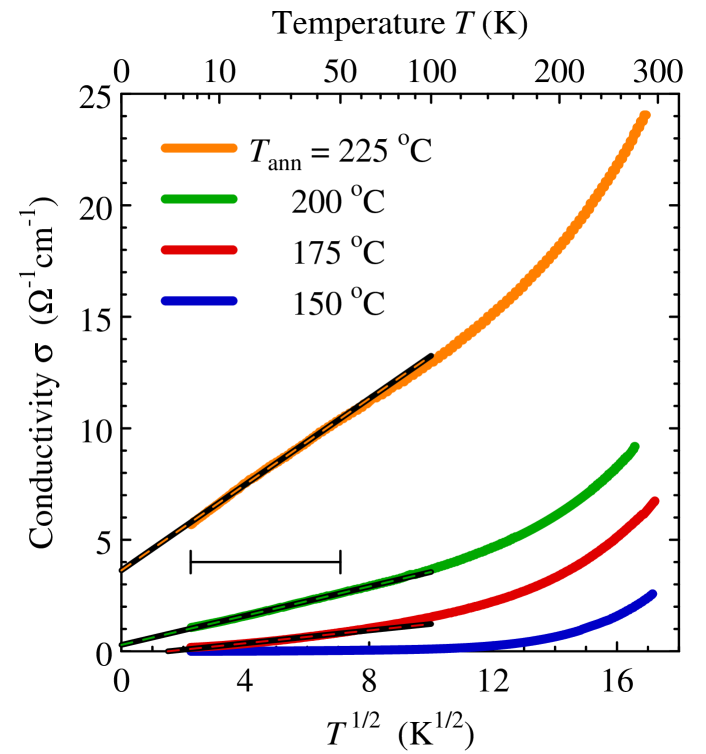
Figure 1: (Color online) Temperature dependences of the conductivity of four GeSb₂Te₄ films redrawn from Figure 3 of Ref. Sie.etal.11, . According to that plot, all these samples are considered as insulating in Ref. Sie.etal.11, . The black straight lines which are overlaid with colored dashes show corresponding $\sigma=a+b\,T^{1/2}$ approximations. The $T$ interval 5 to 50 K taken into account in adjusting the respective parameters $a$ and $b$ is marked by a horizontal bar.

To elucidate this problem, we now evaluate in detail $\rho(T)$ data for GeSb₂Te₄ from Figure 3 of Ref. Sie.etal.11, . For this aim, we digitized the curves for the four lowest annealing temperatures, $T_{\rm ann}=150$, 175, 200, and $225\ {\rm{}^{o}C}$. They are redrawn in a $\sigma$ versus $T^{1/2}$ plot in our Figure 1. This graph tests for the relation $\sigma(T)=a+b\,T^{1/2}$, the Altshuler-Aronov case of the augmented power law, Eq. (2).Alt.Aro.79 Corresponding regression lines which incorporate all data points from one temperature decade, 5–50 K, are included in Figure 1.

For $T_{\rm ann}=200$ and $225\ {\rm{}^{o}C}$, the regression lines seem to nicely approximate the experimental data, not only in the temperature range that was used in adjusting the parameters, but even beyond it up to roughly 100 K. (One should not overestimate the fit quality for $T_{\rm ann}=175\ {\rm{}^{o}C}$, since these $\sigma$ values are so small that the substantial relative deviations are not noticeable in Figure 1.) Note that, for $T_{\rm ann}=225\ {\rm{}^{o}C}$, the $\sigma=a+b\,T^{1/2}$ extrapolation yields $\sigma(T=0)=3.6\ {\rm\Omega^{-1}cm^{-1}}$. This value is smaller by a factor of 100 than the estimate of the minimum metallic conductivity for GeSb₂Te₄ by means of the $\mbox{d}\rho/\mbox{d}T=0$ criterion in Ref. Sie.etal.11, , 300 to $500\ {\rm\Omega^{-1}cm^{-1}}$.

In the augmented power law approach, the MIT is indicated by $a=0$, see Subsection 2.3. Thus, according to our Figure 1, the critical value of $T_{\rm ann}$ should amount to roughly $200\ {\rm{}^{o}C}$. This value deviates considerably from the result $275\ {\rm{}^{o}C}$ which was obtained in Ref. Sie.etal.11, by means of the $\mbox{d}\rho/\mbox{d}T=0$ criterion. Therefore, the question arises how to classify the samples annealed at temperatures in between these two values, in particular the sample obtained by annealing at $225\ {\rm{}^{o}C}$: According to our Figure 1, it should be metallic, but Figure 3 of Ref. Sie.etal.11, suggests that it is presumably insulating.

One and a half years after a first preliminary version of this review had been made available at arXiv.org, see Ref. Moe.13, , three of the authors of Ref. Sie.etal.11, submitted a subsequent study of the MIT in GeSb₂Te₄, Ref. Vol.etal.15, . – Apparently, in Refs. Sie.etal.11, and Vol.etal.15, , (almost) identical sample preparation procedures were used, compare the preparation details given in the Supplementary Information of Ref. Sie.etal.11, and in Section 2 of Ref. Vol.etal.15, with each other. – The authors of Ref. Vol.etal.15, not only extended the explored $T$ range by one order of magnitude down to 0.35 K but also changed their interpretation approach: In locating the MIT, they attached particular importance to the $\sigma=a+b\,T^{1/2}$ approximation, now trusting in it as “the most widely accepted extrapolation method”.Vol.etal.15 Indeed, Figure 2 of Ref. Vol.etal.15, shows that, again, this ansatz works rather well. Thus it supports our above conclusion on the good quality of $\sigma=a+b\,T^{1/2}$ approximations of part of the data published in Ref. Sie.etal.11, . Simultaneously, it yields that the critical annealing temperature should fall between 200 and $225\ {\rm{}^{o}C}$, but closer to the former value. This result only slightly exceeds our above estimate of roughly $200\ {\rm{}^{o}C}$ obtained from the $\sigma(T)$ in Ref. Sie.etal.11, .

Hence, together, Refs. Sie.etal.11, and Vol.etal.15, form a prime example of the decisive influence of the MIT criterion used on the character of the MIT derived. However, not mentioning the reinterpretation of their previous data in Ref. Moe.13, , although citing that source, the authors of Ref. Vol.etal.15, implicitly ascribe their altering the MIT characterization which they had concluded in Ref. Sie.etal.11, only to the focus on the lowest $T$ decade. This way, they hide the interpretation ambiguity from the reader.

Nevertheless, the $\sigma=a+b\,T^{1/2}$ approximations are not perfect. The authors of Ref. Vol.etal.15, point to the weak curvature of their $\sigma$ versus $T^{1/2}$ plots limiting the applicability range of the augmented power law; they mention similar findings for the alternative exponent $1/3$. This feature is not specific to the lowest $T$ decade of their study, which was not taken into consideration in Ref. Sie.etal.11, , and thus also not in the above examination of that work. One can already note it carefully inspecting the curve for $T_{\rm ann}=225\ {\rm{}^{o}C}$ in our Figure 1. A detailed investigation of such weak deviations will be presented for the example of crystalline Si:P in Subsection 4.2.

To gain additional information for the controversial classification of the $\sigma(T)$ data from Ref. Sie.etal.11, , we now study the $T$ dependence of the logarithmic derivative $w$, defined by Eq. (6) above. Figure 2 shows $w(T)$ for the four samples already considered in Figure 1. It compares results obtained by direct numerical differentiation of the experimental data with functions derived from analytic differentiations of various fits to the experimental $\sigma(T)$.

The numerically calculated $w(T)$ points were obtained from the $\ln T(\ln\sigma)$ relations as follows: Sliding a $\ln\sigma$ window along the curve, we calculated the slope by means of linear regression. In this procedure, we related the respective value of the slope to that $\ln\sigma$ value where the truncation error is particularly small, that means, where it is only of second order in the width of the $\ln\sigma$ window; for a detailed explanation see Appendix C. To determine the corresponding value of $\ln T$, we used linear regression. In the present case, numerically calculating $1/w=\mbox{d}\ln T/\mbox{d}\ln\sigma$ instead of $w$ was advantageous with respect to finding a window width which is almost optimal simultaneously at low and high $T$. This width was chosen as small as possible, but so large that digitization effects and random errors are of negligible influence. The values 0.30, 0.15, 0.15, and 0.10 were used for $T_{\rm ann}=150$, 175, 200, and $225\ {\rm{}^{o}C}$, respectively. To ensure that the width of the related $T$ interval does not fall below 1.75 K, the $\ln\sigma$ window was correspondingly expanded if necessary.

The reliability of this procedure was checked in two different ways: First, for $T_{\rm ann}=150\ {\rm{}^{o}C}$, additionally, the $\sigma(T)$ data were also reconstructed from the $\log\rho$ versus $T^{-1/4}$ plot in Figure 8s of the Supplementary Information of Ref. Sie.etal.11, . At low $T$, this graph has a far better resolution than Figure 3 of Ref. Sie.etal.11, . Thus, $w(T)$ could be determined using a $\ln\sigma$ window of width 0.3 over the whole $T$ range, without the occasional interval expansion mentioned above. Figure 2 shows that both the independently obtained $w(T)$ curves for $T_{\rm ann}=150\ {\rm{}^{o}C}$ nicely agree with each other. Second, several unusual patterns of the curves were analyzed. For example, in the case of $T_{\rm ann}=150\ {\rm{}^{o}C}$, the minimum at 63 K turned out not to be an artifact of the digitization but to originate from an offset of the parts of the curve below 61 K and above 65 K by roughly 1 K. This offset is also visible in a large magnification of the original graph. Hence, although the published $\sigma(T)$ data are sufficiently precise for an overview, they exhibit artifacts which substantially influence $w(T)$. Therefore one should be cautious in judging the abnormal features of $w(T)$ discussed in the following.

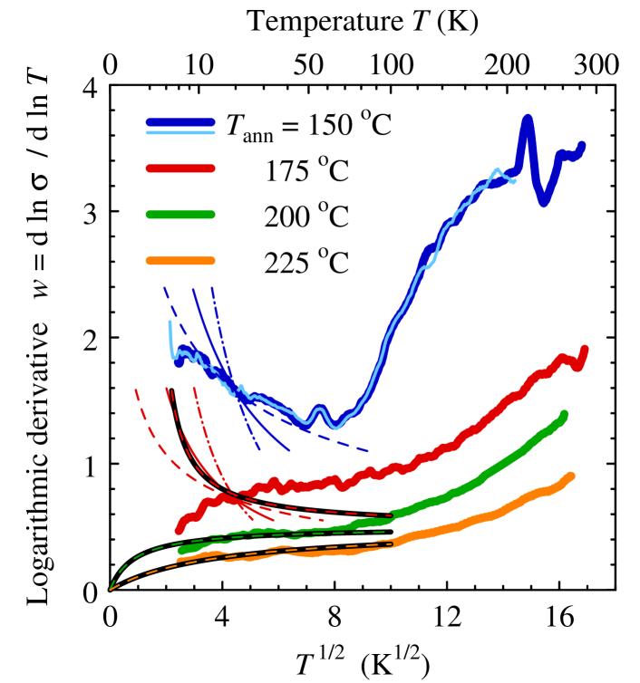
Figure 2: (Color online) Temperature dependences of the logarithmic derivative of the conductivity, $w$, for the four GeSb₂Te₄ data sets shown in Figure 1. For $T_{\rm ann}=150\ {\rm{}^{o}C}$, these values (dark-colored) are compared to data resulting from Figure 8s of the Supplementary Information of Ref. Sie.etal.11, (light-colored), see text. Black curves overlaid with colored dashes correspond to the regression lines in Figure 1. They indicate metallic behavior if $w\rightarrow 0$ as $T\rightarrow 0$. To check for activated transport, dashed, full, and dashed-dotted thin lines give approximations of $w(T)$ by Eq. (9) for $\nu=1/4$, $1/2$ and 1, respectively, see text.

Figure 2 compares the curves obtained by numerical differentiation from the reconstructed experimental data with several theoretical approximations: The dashed, full, and dashed-dotted thin lines relate to activated transport in insulating samples according to Eq. (4) with $\nu=1/4$, $1/2$, and 1, respectively. The corresponding expressions for $w(T)$ include only one adjustable parameter, $T_{0}$, see Eq. (9). Thus, to compare with the experimental data, the values of $T_{0}$ were chosen such that $w(20\ {\rm K})$ agrees with the result of numerical differentiation. The black curves overlaid with colored dashes are based on the Altshuler-Aronov approximation for metallic samples, Eq. (2) with $p=1/2$. They result from analytic differentiation of the regression curves in Figure 1.

We now discuss Figure 2 in detail. For $T_{\rm ann}=200$ and $225\ {\rm{}^{o}C}$, within a wide $T$ range, the curves obtained by numerical differentiation of the $\sigma(T)$ data agree rather well with the analytically differentiated $\sigma=\ a+b\,T^{1/2}$ regressions. Thus, the impression from Figure 1 is supported that already annealing at 225 ${\rm{}^{o}C}$ should be sufficient to reach clearly metallic behavior. Hence, from this perspective, the MIT seems to be continuous, at variance with Ref. Sie.etal.11, .

For $T_{\rm ann}=150\ {\rm{}^{o}C}$, the low-$T$ part of $w(T)$ clearly indicates activated transport due to its negative slope, as expected. In this case, below roughly 50 K, the interpretation in terms of variable-range hopping of Mott type (Eq. (4) with $\nu=1/4$) by Siegrist et al. seems to be confirmed. However, significant deviations are visible below 9 K. The shape of $w(T)$ suggests that they are presumably not real but originate from experimental inaccuracies. Note, moreover, the qualitative change of $w(T)$ at roughly 50 K. The positive slope of $w(T)$ above 50 K is not compatible with any description of a hopping mechanism by Eq. (4). However, such a behavior is not unusual: It points to a second mechanism contributing,Moe.etal.85 ; Moe.85 ; Moe.etal.99 compare also Subsection 4.5, devoted to crystalline CdSe:In.

So far so good, but what about the measurements on the sample annealed at $175\ {\rm{}^{o}C}$? For this sample, the findings are confusing: It should exhibit activated transport according to the unphysical $\sigma(T\rightarrow 0)$ extrapolation in Figure 1. (The corresponding $\sigma=a+b\,T^{1/2}$ fit implies a divergence of $w(T)$ at finite $T$, indicated by the black line overlaid with red dashes in Figure 2.) Hence, in the low $T$ region, the slope of $w(T)$ should be negative as for the three shown approximations for activated transport according to Eq. (9). In fact, however, the slope of the $w(T)$ curve obtained by numerical differentiation of the $\sigma(T)$ data is positive down to the smallest $T$ considered. This discrepancy raises serious doubts about the consistency of all the sample classifications obtained from the $\sigma=a+b\,T^{1/2}$ fits in Figure 1.

How could one understand the contradiction? On the one hand, the temperature might not be low enough. This would be the case if the above mentioned high-$T$ mechanism had a strong influence even at temperatures of a few K. Consequently, for the samples annealed at 200 and $225\ {\rm{}^{o}C}$, the usual $\sigma=a+b\,T^{1/2}$ fits in Figure 1 would be applicable only by chance. Moreover, also the Mott variable-range hopping behavior for $T_{\rm ann}=150\ {\rm{}^{o}C}$ would not be generic but result from the superposition of two mechanisms.

Another possibility is that the exponent of the augmented power law might increase when the MIT is approached. Thus, the simple $\sigma=a+b\,T^{1/2}$ extrapolation procedure might erroneously classify a metallic sample as insulating. However, such a considerable increase of $p$ in the vicinity of the MIT seems to contradict the common experience with other disordered solids, compare Subsection 2.3 and Section 4.

On the other hand, the positive slope of $w(T)$ at low temperatures for $T_{\rm ann}=175\ {\rm{}^{o}C}$ might also be caused by various experimental problems such as incomplete thermalization, Joule heating, or sample inhomogeneities. The low-$T$ deviations for $T_{\rm ann}=150\ {\rm{}^{o}C}$ mentioned above point in this direction. They may originate from a continuous resistance measurement with too fast sliding temperature. A more clear picture will probably be gained when, for a comparably small number of $T$ values, the resistance is always measured only after careful thermalization.Moe.etal.99 Of course, the effect of such an improvement of the measurement has to be checked for all samples. In particular, it will be intriguing to see how, for $T_{\rm ann}=200\ {\rm{}^{o}C}$ and $225\ {\rm{}^{o}C}$, the seemingly good agreement between measured data and regression lines in Figure 1 and between numerically and analytically obtained $w(T)$ curves in Figure 2 will be influenced. Will it persist or disappear?

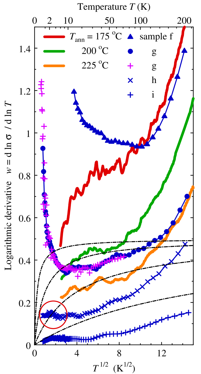
Figure 3: (Color online) Comparison of temperature dependences of the logarithmic derivative of the conductivity, $w$, obtained from two consecutive studies of GeSb₂Te₄. The three curves marked by the respective annealing temperatures are a zoom-in of Figure 2. They were obtained from Ref. Sie.etal.11, ; for explanations see the caption of Figure 2 and the related text. The data sets for the samples f, g, h, and i, marked blue, were obtained from the subsequent publication Ref. Vol.etal.15, by means of digitizing Figures 1 and 2 therein and calculating $w(T)$ numerically, see text; as precision check, data for sample g, marked by magenta $+$ here, were redrawn from Figure 3 of Ref. Vol.etal.15, . These four samples had been annealed at 175, 200, 225, and $250\ {\rm{}^{o}C}$, respectively. For comparison with theory, the dashed-dotted lines represent $w(T)$ resulting from hypothetical $\sigma=a+b\,T^{1/2}$ with $a/b=1/4$, 1, 4, and 16 (from top to bottom).

A first answer to this question is given by Figure 3 of the subsequent publication Ref. Vol.etal.15, , already pointed to above. It presents $w(T)$ curves derived from measurements on GeSb₂Te₄ films down to 0.35 K. To simplify the comparison of our Figure 2 with that diagram, we here condense $w(T)$ data sets obtained from both the Refs. Sie.etal.11, and Vol.etal.15, in a common plot, Figure 3. For this aim, we digitized Figures 1 and 2 of Ref. Vol.etal.15, and calculated the corresponding $w(T)$ sliding windows containing eight neighboring data points along the $\ln\sigma(\ln T)$ curves of the samples f, g, h, and i; these films had been annealed at 175, 200, 225, and $250\ {\rm{}^{o}C}$, respectively. Additionally, as precision check of our procedure, Figure 3 includes data points of sample g obtained by digitizing the $w(T)$ presented in Figure 3 of Ref. Vol.etal.15, .

Our Figure 3 contains a lot of valuable information as we will see in this and the next four paragraphs. Note, above about 140 K, both the $w(T)$ for $T_{\rm ann}=175\ {\rm{}^{o}C}$ from Refs. Sie.etal.11, (old) and Vol.etal.15, (new) agree rather well with each other. The same can be said about the two $w(T)$ curves for $T_{\rm ann}=225\ {\rm{}^{o}C}$ from Ref. Sie.etal.11, and for $T_{\rm ann}=200\ {\rm{}^{o}C}$ from Ref. Vol.etal.15, . On the contrary, below about 100 K, the respective old and new curves qualitatively differ from each other: While the old $w(T)$ seem to decrease with $T$ down to the lowest $T$ taken into account in such a way that both the corresponding samples should be metallic, see above, the new $w(T)$ clearly increase with decreasing $T$ at the lower end of the $T$ range considered which indicates non-metallic conduction. Based on the common assumption that the new data are more precise than the old ones, we conclude that experimental artifacts are the most likely origin of the unusual behavior of the old $w(T)$ for $T_{\rm ann}=175\ {\rm{}^{o}C}$, discussed above. Simultaneously, we mention that, according to the $w(T)$ of sample g, doubts also arise about the low-$T$ decrease of the $w(T)$ of the old sample annealed at $200\ {\rm{}^{o}C}$.

In consequence of their low-$T$ upturns, both the $w(T)$ of samples f and g exhibit minima. They occur at about 100 K for sample f, annealed at $175\ {\rm{}^{o}C}$, and at roughly 12 K for sample g, annealed at $200\ {\rm{}^{o}C}$. Thus, this $T$ value seems to decrease as the MIT is approached. Such a behavior is already known from a-Si_1-xCr_x and a-Si_1-xNi_x;Moe.Adk ; Moe.etal.99 moreover, it is present also in the case of crystalline CdSe:In as will be shown in Section 4.5.

The crucial point now is the following: According to $w(T)$, sample g is clearly non-metallic. Its minimum $w$ value, however, falls considerably below 1/2; it amounts to about 0.35. This finding is incompatible with the hypothesis of a continuous MIT at which $\sigma\propto T^{1/2}$ since $w(T={\rm const.},T_{\rm ann})$ decreases monotonically with increasing $T_{\rm ann}$; see Subsection 2.6.

This conclusion is supported by the behavior of $w(T)$ for sample h. In this case, $w(T)$ seems to be roughly constant below about 20 K; $w$ amounts to 0.14 in this $T$ range. Focusing on the diagram region highlighted by a red circle, one sees that this feature is clearly inconsistent with the properties of the $w(T)$ curves resulting from hypothetical $\sigma=a+b\,T^{1/2}$ for several values of the quotient $a/b$, which is the only adjustable parameter here. Therefore, the $T\rightarrow 0$ extrapolation by means of this ansatz in Ref. Vol.etal.15, , yielding $a=11.2\ {\rm\Omega^{-1}cm^{-1}}$ so that sample h should be metallic, cannot be trusted. – It is strange that this problem was not mentioned in that work. – Even worse, according to our Figure 3, it is not justified to conclude that the $w(T)$ of sample h vanishes as $T\rightarrow 0$. For both these reasons, the classification of this sample as metallic in Ref. Vol.etal.15, is presumably not correct. Because, however, just this classification is basic to the central statement of Ref. Vol.etal.15, that the MIT is most likely continuous, this main conclusion of that publication has to be called into question as well.

Finally, concerning sample i, annealed at $250\ {\rm{}^{o}C}$ and considered as clearly metallic in Ref. Vol.etal.15, , we point to the apparent knee in $w(T)$ at about 4 K. It could be interesting to check this unusual feature by repeating the measurements with lower current and increased precision.

Concluding, taken as a whole, the situation is paradoxical: On the one hand, our analysis of the $\sigma(T)$ data published in the original study, Ref. Sie.etal.11, , in which Siegrist et al. had claimed the MIT to be discontinuous, showed that the ansatz $\sigma=a+b\,T^{1/2}$ seems to work nicely: It yields reasonable descriptions of experimental $w(T)$ for two samples which were classified as insulating in Ref. Sie.etal.11, . This finding is not consistent with the sample classification in that work and might be an indication of the MIT being continuous. On the other hand, in the subsequent publication, Ref. Vol.etal.15, , the explored $T$ range was extended by one order of magnitude down to 0.35 K and the measurement precision was apparently improved. Therein, the authors state the MIT to be most likely continuous and make use of the ansatz $\sigma=a+b\,T^{1/2}$. However, the $w(T)$ curves presented in Figure 3 of that work and the ones in our Figure 3 clearly imply that this ansatz is not applicable in the immediate vicinity of the hypothetical MIT. Thus the continuity of the MIT is called into question.

These contradictions highlight how the “common wisdom” interpretation bias can play a subtle but decisive role in MIT studies. In Section 4, we will show that also numerous publications on the MIT in various other disordered solids suffer from such bias problems. In doing so, considering different choices of the control parameter, $x$, we will identify the likely generic features of the $w(T,x={\rm const.})$ flow diagrams for the vicinity of an MIT.

3.2 Critical charge carrier concentration

The second argument based on which Siegrist et al.Sie.etal.11 ascribe an “unparalleled quantum state of matter” to GeSb₂Te₄ is the allegedly strong deviation of their data from the Mott criterion,Edw.Sie.78

$$n_{\rm c}^{\ 1/3}a_{\rm H}^{\ *}=0.26\pm 0.05\,.$$ (10)

This universal relation links the critical charge carrier concentration, $n_{\rm c}$, at the MIT to the effective Bohr radius, $a_{\rm H}^{\ *}$, of the localized states. Its structure – without specific value at the right-hand side – follows already from a dimensional analysis, see Appendix A. Originally, such a criterion was derived by Mott.Mott.56 Later, Edwards and Sienko extended its applicability by incorporating more realistic wave functions of the localized states, see Ref. Edw.Sie.78, , especially Table I as well as Figure 1 therein. In that work, the simple estimate of $a_{\rm H}^{\ *}$ originally used, which incorporates only the effective electron mass and the permittivity, was refined.

Figure 5 of Ref. Sie.etal.11, depicts the claimed discrepancy between Eq.  (10) and the experimental finding. Siegrist et al. comment on this deviation in a firm manner: “This estimate fails completely for GeSb₂Te₄, where the observed critical carrier concentration at the MIT determined by Hall measurements is $2.0\times 10^{20}\ {\rm cm}^{-3}$. This carrier concentration reproduces the observed minimum metallic conductivity. This consistently indicates that the critical charge carrier concentration is more than a factor of 25,000 larger than the Mott prediction! We are not aware of any other solid where a similar deviation has been observed.”Sie.etal.11

This statement, however, is based on a highly questionable assumption: Siegrist et al. presume that the transport proceeds via shallow impurity states. Only the wave functions of such states may have an extension of more than 100 Å. In contrast, the wave functions of defect states deep in the gap are far more localized. Unlike Siegrist et al., we think it is very likely that these deep states govern the electrical conduction process in GeSb₂Te₄. Our interpretation is supported by the following series of independent arguments.

According to Yu and Cardona, see chapter 4.2.2 in Ref. Yu.Ca, , impurity levels tend to be shallow if the cores (atom minus its outer valence electrons) of host and impurity atoms resemble each other. If, however, the defect induces a substantial strongly localized potential, the arising central cell corrections usually cause the corresponding impurity level to be a deep one. Vacancies belong to the second of these two classes of crystal imperfections. How they give rise to deep levels is discussed in chapter 4.3 of Ref. Yu.Ca, , see also Figure 4.5 therein.

In this context, it is noteworthy that Siegrist et al. conclude from their measurements that the concentration of vacancies in GeSb₂Te₄ is high, see Figure 6a in Ref. Sie.etal.11, and the last but one paragraph on page 4 of the Supplementary Information of Ref. Sie.etal.11, . In the latter, the authors state “… the empty lattice sites play a crucial role in reducing the electrical conductivity in these phase-change materials.” Hence, the concentration of deep levels in the gap should be high and substantially affect the electronic transport.

The influence of vacancies on the electronic structure of various configurations of GeSb₂Te₄ was recently investigated by Zhang et al. by means of density functional theory calculations.Zhang.etal.12 These authors showed that a high concentration of vacancies implies a high density of states at the Fermi energy. Studying the inverse participation ratio of the cubic GeSb₂Te₄ phase with random occupation, they observed that these states are localized to regions of only 25–60 atoms. Their volume is smaller by orders of magnitude than the spatial extension of a shallow impurity state.

The annealing process in Ge₂Sb₂Te₅ films, a related material, was studied by Kato and Tanaka.Kato.Tana They concluded that, in the face-centered cubic phase, the chemical potential is situated 0.15 eV above the valence band edge.Kato.Tana This value is considerably larger than the excitation energy of a shallow doping level, estimated as 8.6 meV in Ref. Sie.etal.11, . Thus, this position of the chemical potential supports the hypothesis that deep levels with strongly localized wave functions play an essential role.

Furthermore, for the following two reasons, it is unlikely that conventional shallow impurity states played an important role in the experiment by Siegrist et al.: (i) Textbook derivations of the properties of a shallow impurity state consider a single impurity in an otherwise perfect infinite crystal. It is therefore questionable to make use of these results in a situation with a very large number of crystal imperfections within the range of the hypothetical shallow donor or acceptor wave function. (ii) Due to the nanocrystalline structure, strain as well as boundary effects may considerably influence the electronic properties of the crystallites. Thus, additional doubts on the applicability of these textbook derivations arise from the grain size of the nanocrystalline GeSb₂Te₄ films being only of the order of 10 to 20 nm, see p. 4 of the Supplementary Information of Ref. Sie.etal.11, . In the case of an effective Bohr radius of 100 Å, the probability density would still have substantial finite values at a grain surface for almost all shallow impurity states.

Our counter-arguments to the interpretation in Ref. Sie.etal.11, which have been presented in the previous paragraphs raise the following question: How does a “standard” material behave in an analogous annealing experiment? Such a study was performed by Song and co-workers for amorphous Si very heavily doped with P or B.Song.etal.10 (For crystalline Si, these elements are typical shallow donors and acceptors, respectively.) These authors deposited a-Si:H films with P and B concentrations of 0.41 and 0.42 atomic percent, respectively. Thus, in both cases, the spatial concentration of the dopants amounts to about $2\times 10^{20}\ {\rm cm}^{-3}$. This value is roughly a factor of 50 larger than the critical concentrations for the MIT in crystalline Si:P and Si:B. Nevertheless, the amorphous films showed clearly activated conduction at room-temperature. Their conductivities amounted to $3.4\times 10^{-4}$ and $1.28\times 10^{-3}\ \Omega^{-1}{\rm cm}^{-1}$, respectively.

In the annealing, the films were dehydrogenated and heavily doped nanocrystalline Si was formed. In this process, the conductivity increased by orders of magnitude up to 5.3 and $130\ \Omega^{-1}{\rm cm}^{-1}$ for the P- and B-doped films, respectively. Simultaneously, the “conductivity activation energy”, $T\mbox{d}\ln\sigma/\mbox{d}\ln T$, decreased by a factor of 10 for P doping and the conductivity almost completely lost its $T$ dependence in the case of B doping. In terms of classifying the character of conduction according to the sign of $\mbox{d}\rho/\mbox{d}T$ at the measuring temperature as in Ref. Sie.etal.11, , this means the MIT had still not been reached in the case of P doping, although the P concentration was so much higher than the critical concentration for crystalline Si:P. However, for B doping, the MIT had probably already almost been reached or even crossed. The findings described here resemble to a large extent the observations in GeSb₂Te₄ by Siegrist et al.. This similarity is a further clear argument against their claim that this phase-change material exhibits an “unparalleled quantum state of matter”.

Song et al. interpret their results in terms of a shift of the Fermi energy due to annealing.Song.etal.10 Simultaneously with the change of the activation energy, the character of the participating states should alter, from deep, strongly localized states toward shallow, far more extended states. In this process, according to Eq. (10), the critical charge carrier concentration, $n_{\rm c}$, decreases. Hence, such an MIT happens primarily due to a variation of $n_{\rm c}$, similar to the MIT caused by applying stress to heavily doped crystalline Si,Tho.etal.83 ; Waf.etal.99 see also Subsection 4.2. The same mechanism should govern the MIT in GeSb₂Te₄, where the transition occurs sometime in the recrystallization process, not at its end.

Summarizing the above arguments, it seems to be very likely that strongly localized states deep in the gap play the crucial role in the transport close to the annealing-induced MIT in GeSb₂Te₄. These states have a far smaller spatial extension than the shallow states. Hence, it is not meaningful to relate the critical charge carrier concentration to the effective Bohr radius of shallow states. In this way, the discrepancy between critical charge carrier density and effective Bohr radius stressed by Siegrist et al. in Ref. Sie.etal.11, is traced back to the authors using an inappropriate value for the latter quantity. Therefore, also concerning the Mott criterion, GeSb₂Te₄ is not special.

4 Comparison with other solids

One might shrug off the ambivalence of the GeSb₂Te₄ measurements discussed above considering them to be ambiguous results for a special, complex material. However, as we will see, contradictory information is also contained in various publications on the MIT in disordered solids which conclude that, at the transition, $\lim_{T\rightarrow 0}\sigma(T,x)$ is a continuous function of the control parameter $x$. To illustrate these contradictions, we now examine several older investigations of crystalline elemental and compound semiconductors, heavily doped with different impurities, as well as recent studies of disordered Gd and nanogranular Pt-C. In this process, to uncover the bias inherent to the usual data evaluations, we analyze in particular the respective $w(T,x={\rm const.})$ flow diagrams; moreover, we demonstrate how, in the augmented power law approach, exponent and temperature range influence the sample classification.

4.1 Crystalline Si:As

First, we turn to crystalline Si:As, an n-type semiconductor, which was studied in great detail by Shafarman et al..Shaf.etal.89 For a series of uncompensated samples with charge carrier concentration, $n$, between $6.85\times 10^{18}$ and $32.8\times 10^{18}\ {\rm cm}^{-3}$, these authors investigated $\sigma(T,n)$ down to 0.5 K. They claimed that, at sufficiently low $T$, the conductivity of their allegedly metallic samples can be well described by $\sigma(T,n)=a(n)+b(n)\,T^{1/2}$. Supposing continuity of the MIT and $\lim_{T\rightarrow 0}\sigma(T,n)\propto(n-n_{\rm c})^{\mu}$ on its metallic side, where $n_{\rm c}$ denotes the critical As concentration and $\mu$ the corresponding critical exponent, Shafarman et al. obtained $\mu=0.60\pm 0.05$; this value is consistent with previous results for Si:P.Shaf.etal.89 ; Tho.etal.83 Close to the MIT, on the insulating side, below 8 K, the authors observed $\sigma(T)$ to be well approximated by Eq. (4) with $\nu=1/4$, which seems to indicate Mott type variable-range hopping.

From the perspective of Section 2, the following points of Ref. Shaf.etal.89, are particularly interesting: According to its Figure 8, at low $T$, while $n$ is varied, $\mbox{d}\sigma/\mbox{d}T$ changes sign when $\sigma\approx 50\ {\rm\Omega^{-1}cm^{-1}}$, in agreement with corresponding Si:P data.Stu.etal.93 ; Ros.etal.81 However, in contrast to previous findings on Si:P,Ros.etal.80 ; Tho.etal.83 none of the possibly metallic Si:As samples has an extrapolated $\sigma(T=0)$ which is smaller than half this value, despite the dense distribution of As concentration values considered: For $n=8.67\times 10^{18}\ {\rm cm}^{-3}$, Figure 8 of Ref. Shaf.etal.89, depicts $\sigma(T=0)\approx 28\ {\rm\Omega^{-1}cm^{-1}}$. For the samples with $n=8.63$ and $8.59\times 10^{18}\ {\rm cm}^{-3}$, whose character Shafarman et al. regarded as not decidable, it is obvious from Figure 11a of Ref. Shaf.etal.89, that $\sigma=a+b\,T^{1/2}$ extrapolations to $T=0$ are problematic due to the considerable curvature of the $\sigma$ versus $T^{1/2}$ plots. Anyway, focusing on the data below 1 K for these two samples, we obtained the estimates $\sigma(T=0)\approx 30$ and $28\ {\rm\Omega^{-1}cm^{-1}}$, respectively. Finally, the sample with the next lower value of the charge carrier concentration, $n=8.48\times 10^{18}\ {\rm cm}^{-3}$, was classified as insulating in Ref. Shaf.etal.89, .

Note, moreover, that for the two samples with $n=8.63$ and $8.59\times 10^{18}\ {\rm cm}^{-3}$, $\sigma$ varies only by roughly 15 % between 0.5 and 4 K. As already remarked in Ref. Shaf.etal.89, , such a $\sigma$ range is much too small to draw reliable conclusions from the alternative stretched exponential fits presented in Figure 11b therein.

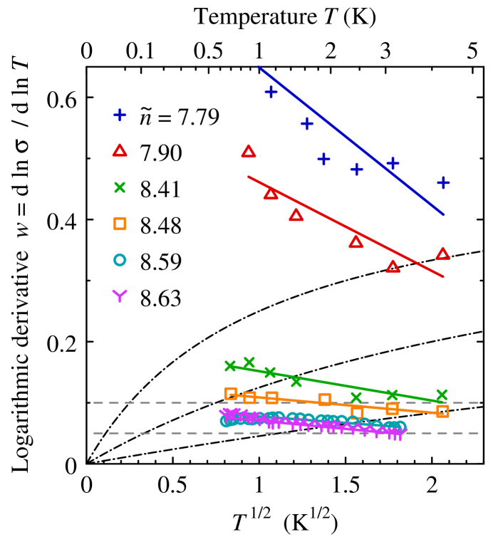
Figure 4: (Color online) Temperature dependences of the logarithmic derivative of the conductivity, $w$, for six crystalline Si:As samples investigated in Ref. Shaf.etal.89, . Here, $\tilde{n}$ indicates the donor concentration as multiple of $10^{18}\ {\rm cm}^{-3}$. The points for $\tilde{n}=7.79$ to 8.48 are redrawn from Figure 4 of Ref. Shaf.etal.89, ; we use the same symbols as in the original plot but another $T$ scale. In addition, points for $\tilde{n}=8.59$ and 8.63 are included which we obtained from the data published in Figure 11b of Ref. Shaf.etal.89, ; see text for details. The straight lines only serve as guides to the eye. The dashed-dotted lines represent $w(T)$ resulting from hypothetical $\sigma=a+b\,T^{1/2}$ with $a/b=1$, 3, and 10 (from top to bottom). To facilitate judging the slope for the samples with the smallest values of $w$, dashed gray lines mark constant $w=0.05$ and 0.1.

In this context, it is very instructive to explore the logarithmic derivative $w(T,n)$ for the Si:As data from Ref. Shaf.etal.89, . Our Figure 4 presents $w(T,n={\rm const.})$ for six samples with $n=7.79$ to $8.63\times 10^{18}\ {\rm cm}^{-3}$. This interval includes the four samples which Ref. Shaf.etal.89, considered as the clearly insulating ones closest to the MIT as well as the two samples which remained unclassified in that study, see above. Partly, the data were redrawn from Figure 4 of Ref. Shaf.etal.89, , partly, they were obtained by digitizing Figure 11b of Ref. Shaf.etal.89, and subsequent numerical differentiation of $\ln\sigma(\ln T)$ based on Appendix C. In these calculations, always, eight neighboring data points were taken into account.

For all samples considered in Figure 4, the inequalities $w>0$ and $\mbox{d}w/\mbox{d}T<0$, on sliding average, hold simultaneously, in clear contradiction to the examples of $w(T)$ curves for hypothetical $\sigma(T)$ following pure augmented power laws. – In fitting the theoretical $w(T)$ to experimental data, there would be only a single adjustable parameter, the ratio $a/b$. Therefore, such a comparison is very meaningful. – Thus, according to Section 2.6, all these samples, including the two samples which could not be classified in Ref. Shaf.etal.89, , are very likely insulating.

Moreover, since $w(T={\rm const.},n)$ decreases with increasing $n$ in the proximity of the MIT, our Figure 4 allows for a conclusion on the separatrix between metallic and non-metallic regions: It is very unlikely that $w(T)\equiv 1/2$ or 1/3 holds at the MIT itself. Hence, for Si:As, it is also very unlikely that $\sigma(T)$ follows a pure power law with exponent 1/2 or 1/3 just at the MIT.

We emphasize that $\mbox{d}w/\mbox{d}T<0$ for all the samples considered in Figure 4 despite of the very weak $T$ dependences of $\sigma$ which a part of them exhibits within the $T$ range studied; for four of them, $w<0.2$, for two of them, even $w<0.1$. Thus, as we will see in Section 5, this diagram is in accord with the hypothesis that $\lim_{T\rightarrow 0}\sigma(T,n)$ is discontinuous at the MIT, whereas, for any $T>0$, $\sigma(T={\rm const.},n)$ is continuous. This hypothesis conflicts with the data analysis by Shafarman et al.Shaf.etal.89 , but it is supported by the above stated lack of possibly metallic Si:As samples with finite $\sigma(T=0)$ extrapolations below half the $\sigma$ value at which, at low $T$, $\mbox{d}\sigma/\mbox{d}T$ changes sign when $n$ is varied.

4.2 Crystalline Si:P

We now consider a similar material, crystalline Si:P, also an n-type semiconductor. It was intensively investigated by groups from Bell Laboratories and from Karlsruhe University down to temperatures of the order of 10 mK, far lower than in the Si:As study considered above. In these Si:P investigations, the MIT was tuned by changing the P concentration, $n$,Ros.etal.80 ; Ros.etal.83 ; Stu.etal.93 and, alternatively, by varying its critical P concentration, $n_{\rm c}$, by applying stress, $S$; thus $n_{\rm c}=n_{\rm c}(S)$.Tho.etal.83 ; Waf.etal.99 In the literature, this series of Si:P studies has been regarded as key experiments confirming the continuity of $\lim_{T\rightarrow 0}\sigma(T,n-n_{\rm c})$ at $n=n_{\rm c}$.Lee.Rama ; Beli.Kirk ; Ever.Mirl

A discontinuity of $\lim_{T\rightarrow 0}\sigma(T,n-n_{\rm c})$ was still not definitely ruled out in the first of these works, Ref. Ros.etal.80, . In the subsequent publications, however, the continuity of $\lim_{T\rightarrow 0}\sigma(T,n-n_{\rm c})$ was implicitly presumed when the measurements were analyzed only by means of the augmented power law ansatz, Eq. (2). In doing so, these analyses paid little attention to the considerable curvature of the $\sigma$ versus $T^{1/2}$ plots being obvious in the respective Figures 1 of Refs. Tho.etal.83, , Waf.etal.99, , and Stu.etal.93, . – In this regard, these diagrams resemble a corresponding plot for crystalline Si:As, Figure 11a of Ref. Shaf.etal.89, , compare previous subsection. – Due to the curvature, the $\sigma(T=0)$ extrapolations significantly depend on which $T$ interval is considered in the $\sigma=a+b\,T^{1/2}$ fits.

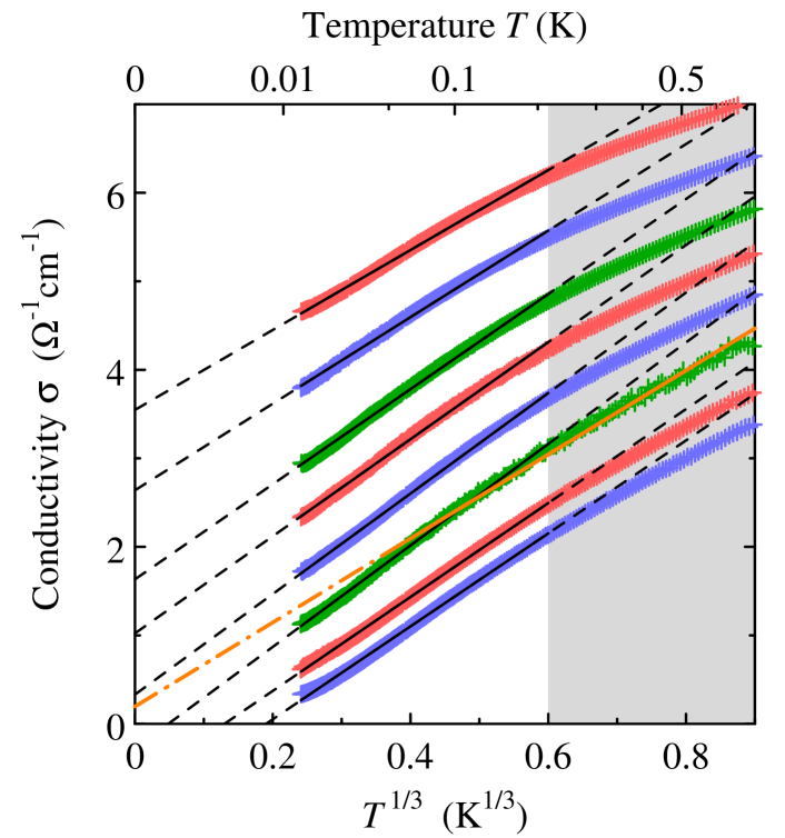
Figure 5: (Color online) Temperature dependences of the conductivity of a Si:P sample with P concentration $3.21\times 10^{18}\ {\rm cm}^{-3}$ under uniaxial stress, $S$, in $\sigma$ versus $T^{1/3}$ representation. The data are redrawn from Figure 1 of Ref. Waf.etal.99, . Compared to Figure 2a of that work, a wider $T$ range is displayed; the part additionally taken into account, 0.216 – 0.729 K, is marked by shading. The same interval of $S$ values as in Figure 2a of Ref. Waf.etal.99, is considered here; from top to bottom, $S=2.00$, 1.94, 1.87, 1.82, 1.77, 1.72, 1.66, and 1.61 kbar; different colors are used to facilitate the inspection of the diagram. (The data of $\sigma(T,1.66\ {\rm kbar})$ are left out in Figure 2a of Ref. Waf.etal.99, .) The black straight lines show respective $\sigma=a+b\,T^{1/3}$ approximations: They are given as full lines within the $T$ interval considered in the fits, 0.014 – 0.216 K as in Figure 2a of Ref. Waf.etal.99, , and as dashed lines in the extrapolation regions outside of it. For comparison, the $a+b\,T^{1/3}$ approximation of $\sigma(T,1.72\ {\rm kbar})$ within the alternative $T$ interval 0.047 – 0.729 K is presented as orange line, full within this interval and dashed-dotted in the extrapolation region.

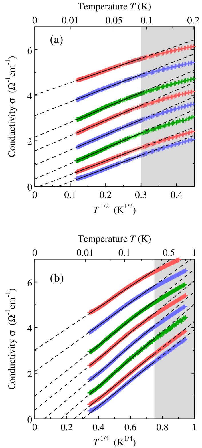
Figure 6: (Color online) Temperature dependences of the conductivity of a Si:P sample under uniaxial stress, redrawn from Figure 1 of Ref. Waf.etal.99, . The same data as in our Figure 5 are shown, but now in (a) $\sigma$ versus $T^{1/2}$ and (b) $\sigma$ versus $T^{1/4}$ representations. Here, the straight lines refer to $\sigma=a+b\,T^{p}$ approximations within the intervals (a) 0.014 – 0.090 K and (b) 0.014 – 0.316 K for $p=1/2$ and $1/4$, respectively; the high-temperature regions not taken into account in these fits are shaded. For further details see caption of Figure 5.

There is one exception among the Si:P studies mentioned above: In the report on their stress tuning of the MIT in Ref. Waf.etal.99, , Waffenschmidt et al. state that, close to the MIT, at low $T$, $\sigma=a+b\,T^{1/3}$ would better describe the experimental data than $\sigma=a+b\,T^{1/2}$. At first glance, this seems to be confirmed by their Figure 2a which shows almost linear $\sigma$ versus $T^{1/3}$ plots for $0.014\ {\rm K}\leq T\leq 0.216\ {\rm K}$; in this representation, the interpolation interval is by a factor of about 1.5 wider than the extrapolation gap. One should note, however, that the impression of a substantial curvature which one gains from the $\sigma$ versus $T^{1/2}$ plots in Figure 1 of Ref. Waf.etal.99, arises under quite other conditions: Therein, the width of the $T^{1/2}$ data range exceeds that of the corresponding low-temperature gap by a factor of about 6.5. Thus, on this basis, a fair comparison of both approximations is impossible.

Therefore, to examine whether the ansatz $\sigma=a+b\,T^{1/3}$ truly better describes the Si:P data published in Ref. Waf.etal.99, than the ansatz $\sigma=a+b\,T^{1/2}$, we now reproduce and extend the augmented power law analysis of these measurements. In doing so, we also aim to find out to what extent the sample classification depends, first, on the $T$ range taken into account in the fits and, second, on the exponent of the augmented power law used.

Our Figure 5 replots $\sigma(T,S)$ data from Figure 1 of Ref. Waf.etal.99, in a $\sigma$ versus $T^{1/3}$ diagram considering the same interval of stress, $S$, as Figure 2a of Ref. Waf.etal.99, , but a wider $T$ range. For clarity, we shaded the $T$ region additionally included into consideration.

Figure 5 shows clearly that substantial deviations from the $\sigma=a+b\,T^{1/3}$ approximations given in Figure 2a of Ref. Waf.etal.99, set in immediately above the $T$ interval taken into account in that diagram, $0.014\ {\rm K}\leq T\leq 0.216\ {\rm K}$. A more detailed inspection leads to the conclusion that precursors of these deviations are already detectable below 0.216 K for $S=2.00$, 1.94, 1.87, 1.82, 1.77, and 1.72 kbar, that means, in particular for the stress values to which the presented augmented power law fits ascribe metallic conduction. Furthermore, our diagram demonstrates for the case $S=1.72\ {\rm kbar}$ that, due to the curvature of $\sigma(T^{1/3})$, the resulting sample classification may depend on the $T$ interval considered in the augmented power law fit. Finally, we draw the reader’s attention to the weak s-shaped deviations of the measured data from the augmented power law approximations in our Figure 5; we will come back to this point later.

As alternative plots, our Figures 6a and 6b present the same data sets in analogous $\sigma$ versus $T^{1/2}$ and $\sigma$ versus $T^{1/4}$ diagrams, respectively; $p=1/4$ is a purely empirical choice. Comparing them with our Figure 5 and with each other is very instructive as is detailed in the following three paragraphs.

First, this comparison makes clear that the sample classification depends to a substantial extent on the exponent value presumed; two, three, and four of the considered $S$ values are classified as belonging to the insulating range for $p=1/2$, 1/3, and 1/4, respectively.

Second, it illustrates the problem that any attempt to find out which value of the exponent, $p$, of the augmented power laws yields the most reliable estimate of $\lim_{T\rightarrow 0}\sigma(T,S)$ is hindered by the uncertainty about the choice of the rating method. There are (at least) three easily accessible figures of merit for such a comparison: mean square deviation, width of the $T$ region considered, and ratio of the width of the interpolation interval to that of the extrapolation gap in the $\sigma$ versus $T^{p}$ plot. – A mathematically strict approach would have to be based on assumptions about $\sigma(T,S={\rm const.})$ which cannot be verified at this stage. – For example, on the one hand, the mean square deviation of the approximations shown in Figure 6a is significantly smaller than that of the fits presented in Figure 5. On the other hand, in Figure 5, the $T$ range taken into account in the fits is considerably wider than that in Figure 6a. The above mentioned ratio of interpolation interval to extrapolation gap, however, is the same in both cases.

Third, the comparison of Figures 5, 6a, and 6b shows that the applicability range of the augmented power law approximation is the wider the smaller the value of $p$. We got support for this finding when we adjusted the parameter $p$ for the individual $\sigma(T,S={\rm const.})$ by numerically minimizing the mean square deviation: For all data sets displayed in Figure 5, the optimum value of $p$ considerably decreases with increasing upper bound of the considered $T$ interval. Moreover, it is noteworthy that this optimum $p$ value varies substantially with $S$, too.

Summarizing the above three points, we have demonstrated how biased interpretations based solely on a single $\sigma$ versus $T^{p}$ diagram are. Furthermore, concerning the examined data sets, we have seen that it is impossible to draw any definite conclusion on the optimum exponent, in contradiction to the interpretation in Ref. Waf.etal.99, . In consequence, it is also not possible to locate the transition point from metallic to insulating conduction in an unambiguous manner by means of the augmented power law approach.

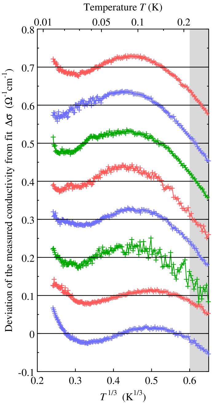
Figure 7: (Color online) Temperature dependences of deviations of the measured $\sigma(T,S={\rm const.})$ for Si:P, published in Ref. Waf.etal.99, , from the corresponding $\sigma=a+b\,T^{1/3}$ approximations shown in our Figure 5. In order to ensure simultaneously high resolution and compact presentation, $\Delta\sigma(T,S)=\sigma(T,S)-a(S)-b(S)\,T^{1/3}+c(S)$ with appropriately chosen values of $c(S)$ is presented here. From top to bottom, $S=2.00$, 1.94, 1.87, 1.82, 1.77, 1.72, 1.66, and 1.61 kbar; the horizontal black lines mark the corresponding $c(S)$. For further details see caption of Figure 5.

Nevertheless, the question arises why, as Figure 5 shows, the $\sigma=a+b\ T^{1/3}$ ansatz can approximate the measured data over more than one decade of $T$ values reasonably well. To clarify this point, our Figure 7 displays a magnification of the weak deviations between measured data and corresponding approximations to which we already pointed in the above discussion of Figure 5.

It is noteworthy that all but one of the curves in Figure 7 have a pronounced s-shape. This feature indicates that the respective $\sigma(T,S={\rm const.})$ exhibit inflection points in the $\sigma$ versus $T^{1/3}$ plot Figure 5. Thus, it is not surprising that $\sigma=a+b\,T^{1/3}$ approximations, corresponding to straight lines therein, seem to work nicely over a rather broad $T$ range in the vicinity of these points.lin_approx

We remark, moreover, that such an s-shape seems not to be consistent with the used ansatz: If a pure $\sigma=a+b\ T^{1/3}$ behavior were approached with decreasing $T$, the deviation should have a parabolic shape at sufficiently low $T$. Thus, also for this reason, the extrapolations to $T=0$ given in Figure 5 have to be called into question.

The problems with the augmented power law analysis described above are another strong motivation for an as unbiased as possible examination of the MIT studies on Si:P. Therefore, we now reanalyze these measurements inspecting the behavior of the logarithmic derivative $w(T,n={\rm const.},S={\rm const.})$. In doing so, we start with considering three experiments in which the MIT was tuned by varying the P concentration, $n$, that is, Refs. Ros.etal.80, , Ros.etal.83, , and Stu.etal.93, .

Our Figure 8 contrasts $w(T,n={\rm const.})$ which we obtained from the data published in these works with curves resulting from hypothetical $\sigma(T)$ obeying augmented power laws, for details see its caption. This diagram shows a more complex behavior than our corresponding Figure 4 on Si:As. The following features of the experimental data are particularly remarkable.

First, there are two $T$ regions with qualitatively different behavior of $w(T,n={\rm const.})$. At high $T$, the $w(T,n={\rm const.})$ have negative slope similar to the Si:As data in Figure 4, whereas, at low $T$, the $w(T,n={\rm const.})$ decrease with $T$ and seem to tend to 0. The transition temperature between both regimes, however, is experiment-specific: It amounts to 0.3 K for the data from Ref. Ros.etal.83, and to roughly 0.1 K for the measurements in Ref. Stu.etal.93, .

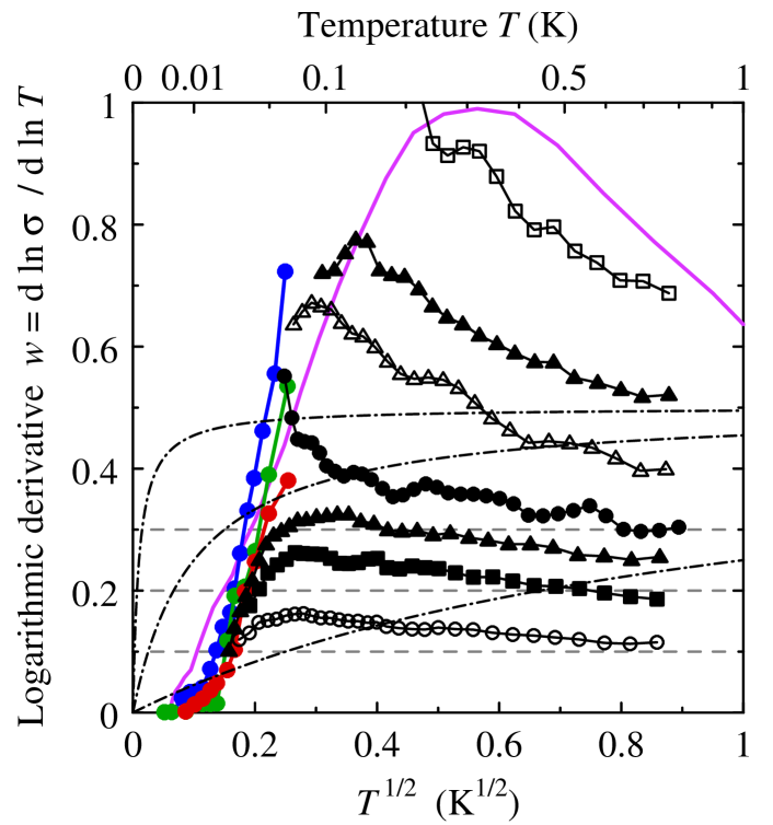
Figure 8: (Color online) Comparison of temperature dependences of the logarithmic derivative of the conductivity, $w$, obtained from three studies on crystalline Si:P in which the MIT was tuned by varying the P concentration, $n$: The colored filled circles result from the three upper curves in Figure 2 of Ref. Ros.etal.80, ; we always considered four neighboring $\ln\sigma(\ln T)$ points in calculating $w$. The magenta line was derived from the curve for $n=3.75\times 10^{18}\ {\rm cm}^{-3}$ in Figure 1 of Ref. Ros.etal.83, . The black symbols result from Figure 1 of Ref. Stu.etal.93, when always five neighboring points are taken into account; from top to bottom, they refer to $n=3.38$, 3.45, 3.50, 3.52, 3.56, 3.60, and $3.67\times 10^{18}\ {\rm cm}^{-3}$. According to the interpretation of Ref. Stu.etal.93, , the upper three of these black curves should correspond to insulating samples, whereas the lower three curves should originate from metallic conduction. The sample to which the medium curve ($n=3.52\times 10^{18}\ {\rm cm}^{-3}$) relates is considered in Ref. Stu.etal.93, to be located very close to the MIT. The dashed-dotted lines represent $w(T)$ which result from hypothetical relations $\sigma=a+b\,T^{1/2}$ with $a/b=0.01$, 0.1, and 1 (from top to bottom). Dashed gray lines mark constant $w=0.1$, 0.2, and 0.3.

Second, the comparison of the experimental data to hypothetical $w(T)$ curves which were obtained from pure augmented power law behavior of $\sigma(T)$, Eq. (2) with $p=1/2$, reveals qualitative discrepancies in both regions: At high $T$, experimental relations and hypothetical curves have slopes of opposite sign; at low $T$, the experimental relations vanish far more rapidly with decreasing $T$ than the hypothetical curves. The latter feature corresponds to the observation in Ref. Ros.etal.83, that the measured $\sigma(T)$ obeys Eq. (2) with $p=2$, which, however, has not been followed up in subsequent publications.

Third, focusing on the data obtained from Ref. Stu.etal.93, , marked by black symbols in Figure 8, we highlight the strong similarity between the $w(T,n={\rm const.})$ of the two groups of samples which were classified in that work as metallic and insulating, respectively; see caption of Figure 8. In particular, we encourage the reader to compare the three middle curves with each other: They result from the data for the samples with $n=3.50$, 3.52, and $3.56\times 10^{18}\ {\rm cm}^{-3}$ which were regarded in Ref. Stu.etal.93, as insulating, as very close to the MIT, and as metallic, respectively.

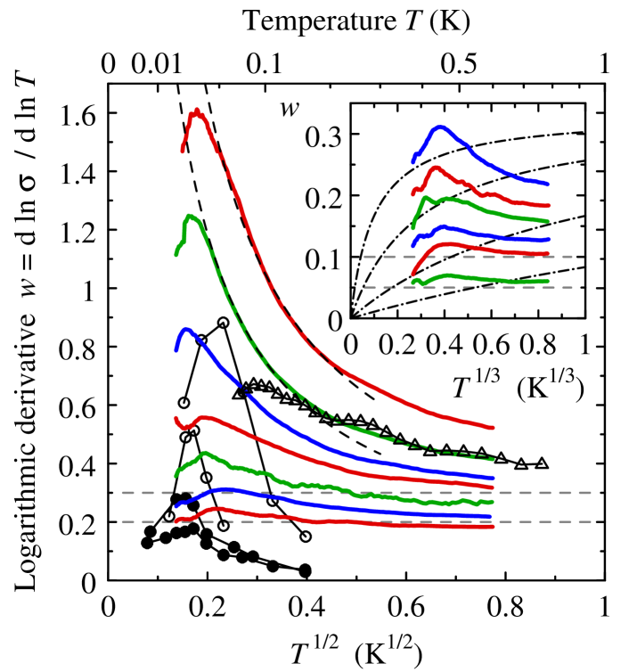
Figure 9: (Color online) Comparison of temperature dependences of the logarithmic derivative of the conductivity, $w$, obtained from two experiments on crystalline Si:P in which the MIT was tuned by varying the critical P concentration by means of stress: The points marked by black circles result from data in Figure 1 of Ref. Tho.etal.83, ; three neighboring $\ln\sigma(\ln T)$ points were considered in each numerical differentiation. From top to bottom, they relate to $S=5.73$, 6.33, 6.59, and 6.71 kbar. The authors of Ref. Tho.etal.83, concluded that the first two $S$ values (empty circles) belong to the insulating range, whereas the latter two values (filled circles) belong to the metallic range. The colored curves were obtained from $\sigma(T,S)$ data presented in Figure 1 of Ref. Waf.etal.99, ; in the calculation of these $w(T)$, we took always 30 neighboring $\sigma(T)$ points into account. From top to bottom, $S=1.50$, 1.56, 1.61, 1.66, 1.72, 1.77, and 1.82 kbar. In Ref. Waf.etal.99, , according to augmented power law fits, only the $\sigma(T,S={\rm const.})$ for the last two stress values were interpreted as indicating metallic conduction. For comparison, data for one sample from Ref. Stu.etal.93, , measured without stress, are included; they are marked by triangles as in our Figure 8. The two dashed black curves represent Eq. (9) for Efros-Shklovskii hopping with $\nu=1/2$; the only free parameter, $T_{0}$, was adjusted at $T=0.1\ {\rm K}$. With enhanced resolution concerning $w$, the inset shows $w(T,S={\rm const.})$ for $S=1.77$, 1.82, 1.87, 1.94, 2.00, and 2.17 kbar obtained from $\sigma(T,S)$ data published in Figure 1 of Ref. Waf.etal.99, . Therein, all these stress values were regarded to belong to the metallic range. In the inset, the data are plotted versus $T^{1/3}$ to facilitate a better test of the approximation $\sigma=a+b\,T^{1/3}$ used in Ref. Waf.etal.99, . The dashed-dotted lines show hypothetical $w(T)$ for this ansatz with $a/b=0.1$, 0.3, 1, and 3. In both plots, gray lines mark constant $w$ to simplify the judgement of the slope of the curves.

Next, we turn to the experiments in which the MIT in Si:P was tuned by means of stress, that is by varying the critical P concentration. Data from such publications by Thomas et al.Tho.etal.83 and by Waffenschmidt et al.Waf.etal.99 are reanalyzed in our Figure 9. The latter measurements seem to be particularly precise; therefore, the detailed discussion of the augmented power law approach in the first part of this subsection focused on them. Here, in Figure 9, the colored curves relate to data published in Ref. Waf.etal.99, . – Also in Ref. phd_waff, , $w(T,S={\rm const.})$ diagrams were derived therefrom. Similarities with and differences to our Figure 9 will be discussed at the end of this subsection. –

In comparing the colored curves with $w(T)$ relations obtained from previous experiments as well as with results from Coulomb glass theory, we made the following observations: (i) On the one hand, down to roughly 0.1 K, there is a nice agreement with a $w(T)$ curve which results from the data in Ref. Stu.etal.93, , measured without stress; the corresponding $\sigma$, however, differ by a factor of about 2.7 at 0.8 K, compare Figure 3 of Ref. Waf.etal.99, and the related discussion in that work. On the other hand, the $w(T)$ obtained from Ref. Waf.etal.99, agree only qualitatively with the $w(T)$ derived from the previous stress tuning of the MIT, Ref. Tho.etal.83, . (ii) In a part of the non-metallic region, for $w\gtrsim 0.7$ and $0.05\ {\rm K}<T<0.1\ {\rm K}$, the colored $w(T)$ can be well approximated by Eq. (9) with $\nu=1/2$ corresponding to variable-range hopping in the Coulomb glass; this finding is of high significance because only one parameter had to be adjusted in each such fit. (iii) As for the measurements without stress discussed above, the $w(T)$ obtained from Ref. Waf.etal.99, exhibit puzzling maxima at low $T$. In this case, however, they occur only at roughly 50 mK, that is at a considerably lower temperature than in the other studies.

Concerning the character of the MIT, two features of the data from Ref. Waf.etal.99, reanalyzed in our Figure 9 are particularly important: First, all these colored $w(T)$ curves show the maxima pointed to above, not only the curves which should be related to metallic behavior according to Ref. Waf.etal.99, , i.e. the curves with $\max(w)<1/3$. Even for the stress values for which $\max(w)>1$, what implies with very high likelihood non-metallic behavior, such maxima are present. Therefore, and because the maxima occur at roughly the same $T$ for all stress values and, moreover, at clearly lower $T$ than in the studies without stress analyzed in Figure 8, we think one should consider the measurements below about 50 mK with caution.

Second, above this temperature, $\mbox{d}w/\mbox{d}T<0$ holds for all curves presented. Thus, according to Subsection 2.6, we regard all these stress values to belong to the insulating side of the MIT. This interpretation is corroborated by the comparison with the hypothetical $w(T)$ obtained from $\sigma=a+b\,T^{1/3}$ in the inset of Figure 9. In Ref. Waf.etal.99, , however, all the measured $\sigma(T)$ from which we obtained the curves in the inset were classified as metallic.

The observation that, above 50 mK, $\mbox{d}w/\mbox{d}T<0$ also when $w$ is clearly smaller than 1/3, even when $w$ is of the order 0.1, accords with the findings for Si:As discussed above. Thus, the same reasoning as for Si:As suggests the hypothesis that Si:P exhibits a discontinuous MIT; but this is in contradiction to the measurements below 50 mK in Ref. Waf.etal.99, .

Finally, for completeness, we refer to the three $w(T,S={\rm const.})$ diagrams in the PhD thesis by S. Waffenschmidt, presented in Figures 4.16 and 4.17 of Ref. phd_waff, ; unfortunately, neither of them was included in the corresponding journal publication, Ref. Waf.etal.99, . These diagrams resemble our Figure 9, but they have less explanatory power for two reasons: The random deviations of the $w(T)$ points in Ref. phd_waff, are considerably larger than those of the points in our Figure 9 because, in Ref. phd_waff, , seven neighboring $\sigma(T)$ points were considered in the calculation of the $w$ values whereas we always took 30 of these very dense data points into account. Furthermore, in the above mentioned diagrams of Ref. phd_waff, , linear $T$ scales are used whereas our Figure 9 presents $w$ versus $T^{1/2}$ and versus $T^{1/3}$. Thus our plots provide better compromises between the demands for a wide $T$ range and a high low-$T$ resolution; moreover, for $p=1/2$ and $1/3$, they have a higher significance in testing of hypothetical approximate $w\propto T^{p}$ for $w\ll p$, as it follows from $\sigma=a+b\,T^{p}$.

Nevertheless, also the lower plot in Figure 4.16 of Ref. phd_waff, shows clearly that, for $0.1\ {\rm K}<T<0.6\ {\rm K}$ and $0.1<w<0.2$, the slope of $w(T)$ is negative, in agreement with our analysis above, but in contradiction to the interpretation in Ref. Waf.etal.99, .

4.3 Crystalline Si:B

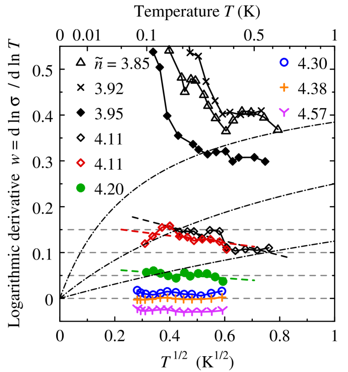
Figure 10: (Color online) Temperature dependences of the logarithmic derivative of the conductivity, $w$, for eight crystalline Si:B samples investigated in Refs. Sara.Dai.02, and Dai.etal.91, . The acceptor concentration $\tilde{n}$ is given as multiple of $10^{18}\ {\rm cm}^{-3}$. The data marked black were obtained by digitizing Figure 1 of Ref. Sara.Dai.02, , while the colored points result from the digitization of Figure 2 of Ref. Dai.etal.91, . For both data sets, always six neighboring $\ln\sigma(\ln T)$ points were considered in the numerical differentiation. The full lines only serve as a guide to the eye, while the black and colored dashed lines arise from linear regression of $w(T^{1/2})$. The dashed-dotted lines represent $w(T)$ resulting from the hypothetical relation $\sigma=a+b\,T^{1/2}$ with $a/b=0.3$, 1, and 3 (from top to bottom). To facilitate judging the slope for the samples closest to the MIT, dashed gray lines mark constant $w=0.$, 0.05, 0.1, and 0.15.

The question arises whether the inconsistencies in the augmented power law approximations of $\sigma(T)$ which have been demonstrated for Si:As and Si:P in the previous two subsections occur only in n-type Si. Therefore, we consider now uncompensated crystalline Si:B. More than two decades ago, this p-type semiconductor was studied by Dai et al. in Ref. Dai.etal.91, in order to obtain the critical exponent of $\lim_{T\rightarrow 0}\sigma(T,n)$ concerning the B concentration, $n$, for the hypothetically continuous MIT.

About ten years later, in Ref. Sara.Dai.02, , two of these authors reported scaling of the $T$ dependences of $\sigma(T,n)$ in the hopping region, compare Subsection 2.5. Therein, they stressed that the scaling curve includes data for three samples interpreted as metallic in their previous work and concluded that additional careful investigations down to “as low a temperature as possible” are required to solve this puzzle.

Our Figure 10 presents $w(T,n={\rm const.})$ relations obtained from the data published in Refs. Sara.Dai.02, and Dai.etal.91, , for details see its caption. This plot resembles our corresponding graph for Si:As, Figure 4, to a large extent as it is explicated in the following two paragraphs.

Consider first the $w(T)$ for the three samples with $n=3.85$, 3.92, and $3.95\times 10^{18}\ {\rm cm}^{-3}$, classified as insulating in Ref. Dai.etal.91, as well as in Ref. Sara.Dai.02, . In all three cases, simultaneously, the smallest value of $w$ falls clearly below 0.5, while, on sliding average, the respective slope $\mbox{d}w/\mbox{d}T$ is obviously negative. As discussed in Subsection 2.6, this finding is incompatible with the hypothesis of a continuous MIT with $\sigma\propto T^{1/2}$ just at the transition.

We now turn to the three samples which were assumed to be metallic in Ref. Dai.etal.91, but regarded as insulating in Ref. Sara.Dai.02, , that means the samples with $n=4.11$, 4.20, and $4.30\times 10^{18}\ {\rm cm}^{-3}$. We emphasize that, on the average, $\mbox{d}w/\mbox{d}T$ is clearly negative for the former two of these samples, notwithstanding that $w$ is far smaller than 0.5, even considerably smaller than 0.2. In consequence, also from the perspective chosen here, these two samples are very likely insulating.

Concerning the third of these samples, $n=4.30\times 10^{18}\ {\rm cm}^{-3}$, a definite conclusion is not possible for us at the current state because the digitized data are not precise enough to reach a reliable decision on the sign of $\mbox{d}w/\mbox{d}T$. We remark, however, that also a scaling analysis as in Ref. Sara.Dai.02, is rather uncertain in this case: The $T$ dependences of $\sigma$ for $n=4.20$ and $4.30\times 10^{18}\ {\rm cm}^{-3}$ are so weak that these curves cannot be made to overlap each other in a mastercurve construction. Therefore, one has to rely on the implicit assumptions discussed in detail in Appendix B. In particular, one has to trust in the mean hopping energy tending to zero as the MIT is approached, that means in $\mbox{d}\sigma/\mbox{d}T=0$ marking the MIT at sufficiently low temperature.

Summarizing this subsection, we conclude that the inconsistencies in the augmented power law approximations of $\sigma(T)$ for heavily doped crystalline Si seem not to be specific to n-type doping. This interpretation is also supported by observations on partially compensated Si:(P,B), see Figures 1 in Refs. Moe.89, and Hir.etal.89, .

4.4 Crystalline ⁷⁰Ge:Ga

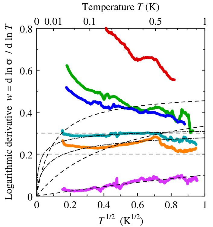
Figure 11: (Color online) Temperature dependences of the logarithmic derivative of the conductivity, $w$, for six crystalline neutron transmutation doped ⁷⁰Ge:Ga samples investigated in Ref. Wata.etal.98, . They are shown as colored curves and relate to Ga concentrations, $n$, of 1.853, 1.856, 1.858, 1.861, 1.863, and $1.912\times 10^{17}\ {\rm cm}^{-3}$, from top to bottom.Wata.etal.98 To obtain these relations, we reconstructed the $\sigma(T,n={\rm const.})$ from Figure 1 of Ref. Wata.etal.98, and differentiated the individual $\ln\sigma(\ln T)$ numerically considering groups of 30 neighboring data points. The dashed and dashed-dotted lines represent $w(T)$ curves resulting from hypothetical $\sigma=a+b\,T^{p}$ with $p=1/2$ and 1/3, respectively. Here, $a/b=0.1$, 0.5, and 4 for $p=1/2$, whereas $a/b=0.08$ and 0.2 for $p=1/3$. To facilitate judging the slope of $w(T)$, dashed gray lines mark constant $w=0.2$ and 0.3.

The next question to answer is: Might the inconsistencies of the augmented power law approximations of $\sigma(T)$ close to the MIT which were pointed out in the previous subsections be specific only to heavily doped Si?

This is not the case as our Figure 11 shows. For six ⁷⁰Ge:Ga samples with different values of the Ga acceptor concentration, $n$, it presents $w(T,n={\rm const.})$ curves which we obtained from data by Watanabe et al. published in Ref. Wata.etal.98, ; for details see caption of Figure 11. These authors used an elaborate sample preparation technique based on neutron transmutation for doping to achieve a high degree of homogeneity;Wata.etal.98 for an earlier MIT study utilizing this technology, see Ref. Zabr.Zino, . Moreover, they applied a two-step irradiation process in order to fine-tune the concentration of Ga acceptors close to the MIT.Wata.etal.98

Watanabe et al. analyzed their data by means of augmented power law fits and interpreted them in terms of a continuous MIT.Wata.etal.98 This way, they classified the samples to which the upper three curves in Figure 11 are related as insulating, whereas they regarded the samples from which the lower three curves result as metallic.Wata.etal.98 Concerning the latter three samples, the authors concluded that $\sigma(T)$ can be well approximated by augmented power laws with $p=1/2$ far from the MIT and $p=1/3$ in its immediate vicinity.Wata.etal.98

To check this interpretation, our Figure 11 contrasts the $w(T,n={\rm const.})$ relations which we obtained by numerical differentiation of the measured $\sigma(T,n={\rm const.})$ with $w(T)$ curves resulting from analytical differentiation of hypothetical $\sigma=a+b\,T^{p}$ with $p=1/2$ and 1/3, evaluated for several values of $a/b$. This graph strongly resembles the corresponding plots in the previous subsections. In detail, we interpret it as follows.

Consider first the sample with the smallest $w$, that is, the sample with $n=1.912\times 10^{17}\ {\rm cm}^{-3}$. In this case, in agreement with Ref. Wata.etal.98, , analytically differentiated $\sigma=a+b\,T^{1/2}$ with $a/b=4$ seems to well approximate the curve obtained from the measured data by numerical differentiation. Note, however, that $w<0.1$ holds for this sample in the entire $T$ range considered here.

Simultaneously, due to the strong discrepancies between the slopes of the numerically calculated $w(T)$ curves and the analytically obtained ones, the hypothesis $\sigma=a+b\,T^{1/2}$ clearly fails for all other samples. In particular, within the region $0.3<w<0.5$, positive slopes of the $w(T,n={\rm const.})$ would be expected if the MIT were continuous and $\sigma$ were proportional to $T^{1/2}$ at the transition itself. In fact, however, on sliding average, $\mbox{d}w/\mbox{d}T$ is negative in this $w$ region. Thus, again, and in agreement with Ref. Wata.etal.98, , the approximation $\sigma=a+b\,T^{1/2}$ is not applicable in the immediate vicinity of the hypothetical MIT.

The question whether or not an augmented power law with $p=1/3$ may be valid close to a continuous MIT cannot be finally decided for ⁷⁰Ge:Ga here because the $\sigma(T)$ data are not precise enough. Nevertheless, at the current stage, there are more cons than pros as is explained in the following three paragraphs.

In trying to answer this question, we focus on the other two samples which were regarded as metallic in Ref. Wata.etal.98, , that is, on the samples with $n=1.861$ and $1.863\times 10^{17}\ {\rm cm}^{-3}$; for them, $0.2<w<0.35$ holds within the $T$ interval studied in Figure 11. In the medium $T$ range of this graph, at first glance, the $w(T)$ obtained by numerical differentiation from the measured data and the results of analytical differentiation of augmented power laws with $p=1/3$ seem to be consistent with each other, in accord with Ref. Wata.etal.98, . However, the substantial deviations between the respective curves which occur at the lower and upper ends of the $T$ interval considered in Figure 11 clearly conflict with this interpretation.

Note, moreover, that the $w(T)$ curves for $n=1.853$, 1.856, and $1.863\times 10^{17}\ {\rm cm}^{-3}$ exhibit unusual bumps at about 0.5 K, presumably resulting from some measurement artifacts. These features raise additional doubts about the plausibility of the seeming consistency in the medium $T$ range for $n=1.861$ and $1.863\times 10^{17}\ {\rm cm}^{-3}$ to which we pointed in the previous paragraph.

Finally, we remark that, on average over the whole $T$ range, $\mbox{d}w/\mbox{d}T$ seems to be slightly negative and approximately zero for the samples with $n=1.861$ and $1.863\times 10^{17}\ {\rm cm}^{-3}$, respectively. Therefore, at least the former sample should actually be insulating in contradiction to the classification in Ref. Wata.etal.98, .

In consequence, since $w(T={\rm const.},n)$ decreases with increasing $n$, the data reconsidered here seem to imply the following conclusion: If the MIT is continuous and $\sigma(T)\propto T^{p}$ at the MIT itself, then $p\lesssim 0.25$; alternatively, the MIT may be discontinuous. Hence, because of the above arguments, the interpretation by Watanabe et al. that $\sigma=a+b\,T^{1/3}$ in the immediate vicinity of the MIT is unlikely to be valid. An improvement of precision and accuracy of these $\sigma(T)$ measurements should be very promising.

4.5 Crystalline CdSe:In

In the previous subsections, we have examined MIT studies of only elemental semiconductors. Now we ask whether the characteristic features of $\sigma(T,n)$ and $w(T,n)$ which we have exposed therein can be identified also in reports on compound semiconductors. First, we turn to n-type CdSe, a II-VI semiconductor. The (actual or alleged) hopping conduction in In-doped compensated CdSe was analyzed from different perspectives in three subsequent publications: In Ref. Zha.etal.90, , Zhang et al. probed the Coulomb gap; they interpreted their measurements in terms of a crossover between $\sigma(T)$ following Eq. (4) with $\nu=1/2$ at low $T$ and Eq. (4) with $\nu=1/4$ at high $T$. Later, reinterpreting and extending these investigations, universality of the crossover and two-parameter scaling were claimed in Refs. Aha.etal.92, and Zha.Sara.95, , respectively. – Refs. Zha.etal.90, and Aha.etal.92, consider the same five samples, but dopant concentration values were redetermined in Refs. Aha.etal.92, . Out of these publications, only Ref. Zha.Sara.95, presents $\sigma$ values in absolute units. –

Remarkably, for the sample with the highest net donor concentration among the ones investigated in Ref. Zha.Sara.95, , $\sigma(T)$ changes only by a factor of about 2.4 over the lowest decade of the $T$ range studied, that is, between 0.062 and 0.62 K, see Figure 1 therein. In terms of simple approximations, this low value can be interpreted in three different ways: (i) In case, the sample was located just at a continuous MIT, so that $\sigma(T)$ followed a pure power law, the quotient 2.4 would correspond to an exponent of roughly 0.4. (ii) If, alternatively, $\sigma(T)$ could be described by the augmented power law Eq. (2) with $p=1/2$, then, in consequence of the ratio 2.4, the constant contribution $a$ would be positive and thus indicate metallic conduction. (iii) Of course, such a low ratio could also result from variable-range hopping described by Eq. (4) with $T_{0}$ being comparable to the $T$ values considered. For $\nu=1/2$ and $1/4$, the ratio 2.4 implies $T_{0}=0.10\ {\rm K}$ and $0.99\ {\rm K}$, respectively; Table I of Ref. Zha.etal.90, reports $T_{0}=0.10\ {\rm K}$ and $0.65\ {\rm K}$, respectively, relating to data for higher temperatures in the latter case.

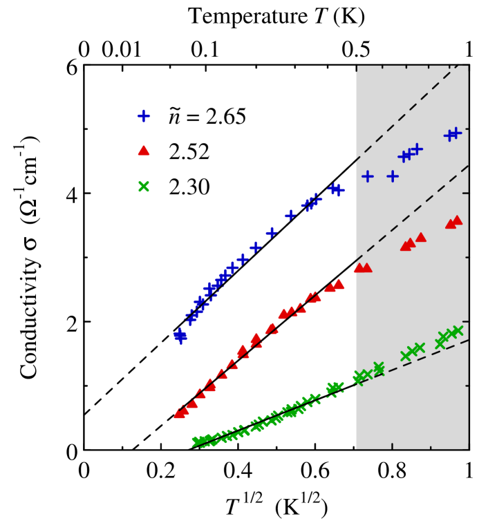
Figure 12: (Color online) Temperature dependences of the conductivity of three CdSe:In samples redrawn from Figure 1 of Ref. Zha.Sara.95, . The values of the net donor concentration, $\tilde{n}$, are given as multiple of $10^{17}\ {\rm cm}^{-3}$; they are taken from Table I of that work. All these samples are regarded as insulating in Ref. Zha.Sara.95, . The straight lines show respective $\sigma=a+b\,T^{1/2}$ approximations: They are given as full lines within the $T$ range considered in the fits, 0.06 – 0.5 K, and as dashed lines in the extrapolation region outside of it. The region above 0.5 K is shaded to simplify the discussion.

Because of this ambiguity, it should be very interesting to find out whether or not $T\rightarrow 0$ extrapolations based on the augmented power law Eq. (2) with $p=1/2$ can be used for the classification of the CdSe:In samples, too, and which result they yield. To clarify these points, we digitized the $\sigma(T)$ data published in Figure 1 of Ref. Zha.Sara.95, focusing on the three samples with the highest net donor concentrations. These data are redrawn in a $\sigma$ versus $T^{1/2}$ plot in Figure 12 here.

When covering the shaded part of our graph, one sees that Eq. (2) seems to be reasonably well fulfilled between about 0.06 and 0.5 K, that means over almost one temperature decade as also in our Figure 1 on GeSb₂Te₄ films. According to the corresponding $T\rightarrow 0$ extrapolations, the CdSe:In sample with the highest net donor concentration, $n=2.65\times 10^{17}\ {\rm cm}^{-3}$, should be metallic in contradiction to the interpretation in Ref. Zha.Sara.95, , while the two others should be insulating in agreement with that work.

Additionally taking the data points between 0.5 and 1 K into account, however, totally changes the situation: The previously obtained augmented power law fits now cease to be good approximations of the experimental data, so that the $T\rightarrow 0$ extrapolation for $n=2.65\times 10^{17}\ {\rm cm}^{-3}$ and the therefrom concluded sample classification are called into question.

The here demonstrated interpretational ambiguity of augmented power law fits to $\sigma(T)$ data sheds bright light on how questionable this approach is for CdSe:In, too. Thus, our Figure 12 shows a further example of the decisive influence of the choice of the MIT criterion on the sample classification obtained.

Note the resemblance between this graph and corresponding plots for Si:P, Figure 1 of Ref. Stu.etal.93, and our Figures 5 and 6. From all these graphs, it is obvious how strongly the usual localization theory motivated augmented power law extrapolation results depend on which $T$ interval is chosen to fit Eq. (2) to the experimental data. Nevertheless, together, these figures support the idea that the character of the MIT should be the same in CdSe:In and Si:P.

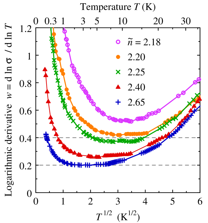
Figure 13: (Color online) Temperature dependences of the logarithmic derivative of the conductivity, $w$, for the five crystalline CdSe:In samples investigated in Refs. Zha.etal.90, and Aha.etal.92, . The values of $w(T,n)$ were obtained from Figure 1 of Ref. Aha.etal.92, as described in the text. The net dopant concentrations $\tilde{n}$, given as multiple of $10^{17}\ {\rm cm}^{-3}$, are taken from Table I of Ref. Aha.etal.92, .

The next question, of course, concerns the behavior of a set of $w(T,n={\rm const.})$ curves for CdSe:In. To answer it, we digitized the $\sigma(T)$ data for five samples published in Figure 1 of Ref. Aha.etal.92, . This graph includes values from a very wide $T$ range, from about 60 mK up to roughly 100 K. Utilizing the numerical differentiation method explained in Appendix C, we calculated $1/w(T,n={\rm const.})$ sliding a $\ln\sigma$ window of width 1.0 along the $\ln T(\ln\sigma)$ curves, analogously to our approach in Subsection 3.1. To guarantee that at least 7 data points are taken into account in each slope calculation, the $\ln\sigma$ window was correspondingly expanded if necessary. This procedure ensures that the random errors of the $w$ values are kept small in the medium temperature range, where $w(T)$ seems to vary only slowly.

The resulting $w(T,n={\rm const.})$ data are presented in Figure 13. Three features of this graph deserve particular attention. First, for $T\lesssim 1\ {\rm K}$, all $w(T,n={\rm const.})$ exhibit negative slope, in agreement with Figure 3b of Ref. Zha.etal.90, . Therefore, we support the sample classification in Refs. Zha.etal.90, ; Aha.etal.92, ; Zha.Sara.95, where all these samples are considered as insulating. Moreover, we point out that the considerable negative slope of $w(T)$ is the origin of the problems with the augmented power law approximations of $\sigma(T)$ discussed above.

Second, in contrast, at high $T$, that means above roughly 15 K, $w$ increases with $T$ for all samples considered here. This behavior very likely arises from a second conduction mechanism yielding a substantial contribution to $\sigma(T)$, see the discussion in Subsection 2.6, compare also Figure 2.

Third, in between the low- and high-$T$ regimes, all $w(T,n={\rm const.})$ exhibit pronounced minima. The corresponding temperature value, $T_{\rm min}(n)$, decreases as $n$ increases, that means as the MIT is approached, and so does $w_{\rm min}(n)=w(T_{\rm min}(n),n)$. – This feature could already be foreshadowed from inspection of Figure 3b of Ref. Zha.etal.90, , restricted to $T\lesssim 10\ {\rm K}$. – Such characteristic minima are not special to CdSe:In, they were observed already in amorphous alloys, see Figure 7 in Ref. Moe.Adk, and Figures 7a/b in Ref. Moe.etal.99, for a-Si_1-xCr_x and a-Si_1-xNi_x, respectively; see also our Figure 3 on GeSb₂Te₄. Finally, we stress that, for the CdSe:In sample closest to the MIT, $w_{\rm min}\approx 0.2$. This is incompatible with the idea of a continuous MIT at which $\sigma(T)\propto T^{p}$ with $p=1/2$ or $1/3$; for the reasoning, see Subsection 2.6.

Concluding this subsection, we encourage the reader to compare Figure 13 to the diagrams in our Section 5. They show the behavior of $w(T,x)$ in the vicinity of the MIT for four simple, qualitatively different phenomenological models of $\sigma(T,x)$, where $x$ stands for an arbitrary control parameter. In our opinion, Figure 13 closest resembles Figure 23. The latter diagram presents a set of $w(T,x={\rm const.})$ curves for a discontinuous MIT which is superimposed by an additional high-temperature conduction mechanism and for which $\mbox{d}\sigma/\mbox{d}T=0$ indicates the transition point in the low-$T$ limit. This resemblance is in accord with the interpretation in Ref. Zha.Sara.95, , where the existence of a finite minimum metallic conductivity was concluded from two-parameter scaling of the $T$ dependences of $\sigma$.

4.6 Crystalline n-Cd_0.95Mn_0.05Se

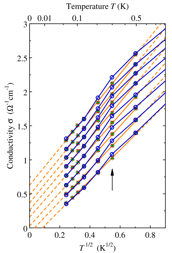
Figure 14: (Color online) Temperature dependences of the conductivity of an n-Cd_0.95Mn_0.05Se sample with net In-donor concentration $4\times 10^{17}\ {\rm cm}^{-3}$ under various magnetic fields published in Refs. Wojt.etal.86, and Dietl.etal.86, ; from top to bottom, $H=28.5$, 25.2, 22.7, 20.2, 17.7, 15.2, 12.7, and 10.3 kOe. The data marked by red $\times$ and green $+$ are redrawn from the apparently identical plots in Figure 1a of Ref. Wojt.etal.86, and Figure 6 of Ref. Dietl.etal.86, ; the data given by blue circles were obtained by digitizing the $\rho(H,T={\rm const.})$ curves in Figure 4 of Ref. Dietl.etal.86, . The orange straight lines refer to $\sigma=a+b\,T^{1/2}$ approximations of the data from Figure 6 of Ref. Dietl.etal.86, for the interval 0.059 – 0.493 K; they are given as full lines within this range and as dashed lines in the extrapolation region outside of it.

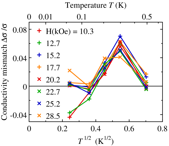
Figure 15: (Color online) Mismatch between the digitized values of the data sets published in Figures 4 and 6 of Ref. Dietl.etal.86, . This diagram presents $(\sigma({\rm Figure\ 4})-\sigma({\rm Figure\ 6}))/\sigma({\rm Figure\ 6})|_{(T,H_{i})}$ versus $T^{1/2}$ for the $H_{i}$ values listed in the caption of Figure 14.

In certain cases, alternatively to utilizing stress, the MIT can also be tuned by applying a magnetic field. Thereby, the variation of the critical dopant concentration can originate from two effects acting in opposite directions: On the one hand, the field squeezes the dopant wave functions and thus increases the critical dopant concentration. On the other hand, the field reduces the effective disorder by partially aligning d-spins which, in turn, affect the current carrying shallow impurity levels via s-d exchange interaction; this way, the field reduces the critical dopant concentration. For details see Refs. Efros.Shkl.84, and Dietl.etal.86, , respectively.

As an example of employing the second of these effects in the study of the MIT, we now evaluate the investigation of the semimagnetic crystalline semiconductor n-Cd_0.95Mn_0.05Se described in Refs. Wojt.etal.86, and Dietl.etal.86, . In these measurements, the magnetic field was directed perpendicular to the current. Thus, interpretation complications can arise from the tensor character of the conductivity. However, the authors of Ref. Wojt.etal.86, claim the magnetoresistance to be isotropic in this case, so that the corresponding corrections should be negligible in the data evaluation. In the following, we take this assumption for granted.

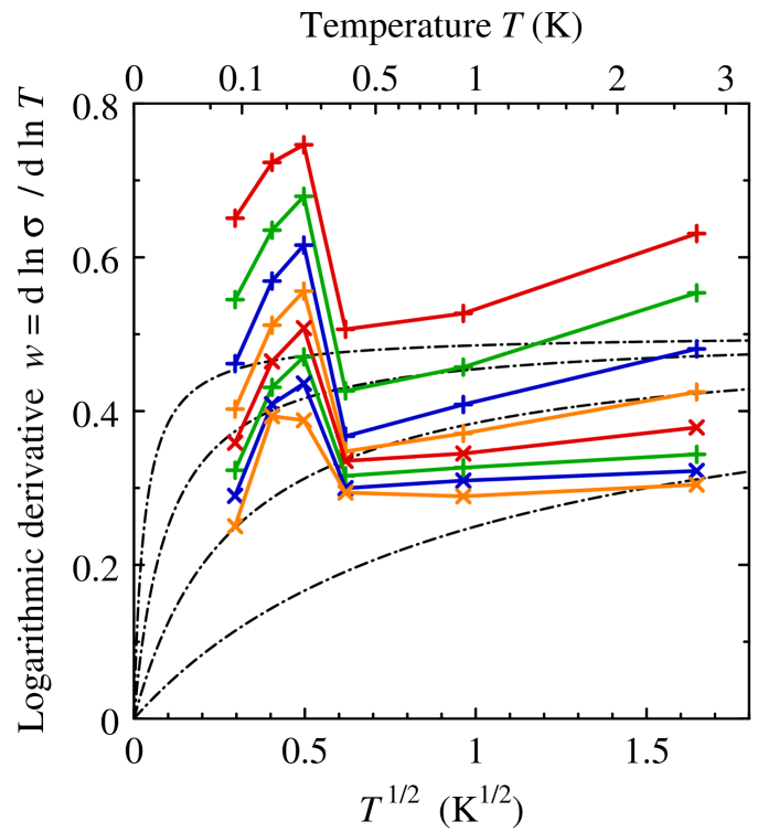
Figure 16: (Color online) Temperature dependences of the logarithmic derivative of the conductivity, $w$, for an n-Cd_0.95Mn_0.05Se sample studied in Ref. Dietl.etal.86, , in which the MIT was tuned by varying the critical dopant concentration by means of magnetic field; compare caption of Figure 14. The data presented here were obtained from Figure 4 of Ref. Dietl.etal.86, ; the symbols have the same meaning as in our Figure 15. For comparison, the dashed-dotted lines represent $w(T)$ resulting from the hypothetical relation $\sigma=a+b\,T^{1/2}$ with $a/b=0.03$, 0.1, 0.3, and 1 (from top to bottom).

To inspect an as broad as possible $T$ range, to ask for the limit of the linear range of $\sigma(T^{1/2},H={\rm const.})$ analogously to our approach in Subsection 4.2, and, moreover, to check our digitization, we took into consideration all available published data. Thus we digitized not only the apparently identical plots of $\sigma(T,H={\rm const.})$ versus $T^{1/2}$ in Figure 1a of Ref. Wojt.etal.86, and Figure 6 of Ref. Dietl.etal.86, , but also the $\log_{10}\rho(T={\rm const.},H)$ versus $H^{1/2}$ diagram Figure 4 of Ref. Dietl.etal.86, , which includes data from a wider $T$ range.

Surprisingly, the digitization precision check uncovered a systematic mismatch between these data sets: Our Figure 14 shows that, in particular, the presumably “more original” data points in Figure 4 of Ref. Dietl.etal.86, mark significantly larger values of $\sigma(0.3\ {\rm K},H)$ than the corresponding data points in Figure 1a of Ref. Wojt.etal.86, and Figure 6 of Ref. Dietl.etal.86, ; this temperature is indicated by an arrow. The first impression is confirmed by the detailed presentation of the mismatch in our Figure 15, showing that this deviation considerably exceeds the random digitization errors. – Of course, we double-checked this finding very carefully. –

Two strange effects may help to evaluate this discrepancy: First, all $\sigma(T^{1/2},H={\rm const.})$ given in Figure 6 of Ref. Dietl.etal.86, can be described almost exactly by $\sigma=a(H)+b(H)\,T^{1/2}$, compare our Figure 14, whereas the $\sigma(T^{1/2},H={\rm const.})$ obtained from Figure 4 of that work exhibit a slight s-shape, similarly to our finding for Si:P in Subsection 4.2. Second, if, instead of the actually presented values, the data from Figure 4 of Ref. Dietl.etal.86, were shown in Figure 6 of that work (or in Figure 1a of Ref. Wojt.etal.86, ), then the quality of the fits to Finkel’stein’s renormalization group equations therein would be considerably damaged. Of course, thirty years after publication, it may be impossible to solve this puzzle. However, in future work, caution is advised in drawing conclusions from Figures 1a of Ref. Wojt.etal.86, and Figure 6 of Ref. Dietl.etal.86, .

What does the logarithmic derivative $w(T,H={\rm const.})$ tell us about this MIT? To answer the question, we calculated $w$ starting from $\ln\sigma(\ln T)$ relations obtained from Figure 4 of Ref. Dietl.etal.86, ; in this case, we considered all pairs of neighboring $T$ values. The results are presented in our Figure 16: Again, the numerically obtained relations differ qualitatively from the $w(T)$ expected according to the hypothetical $\sigma=a+b\,T^{1/2}$. As for Si:P, all $w(T,H={\rm const.})$ exhibit maxima at roughly the same temperature, at about 0.2 K in the present case. Such a maximum occurs even for the field strength $10.3\ {\rm kOe}$ which, according to the corresponding maximum value of $w$, as well as to Ref. Dietl.etal.86, , should clearly fall into the insulating region. Furthermore, above this temperature, up to 0.4 K, a considerable decrease of $w$ with increasing $T$ is present also for the $H$ values interpreted as belonging to the metallic region in Ref. Dietl.etal.86, , even for the largest field, for which $w$ falls down to about 0.3. Therefore, although we consider these data with caution due to the discrepancies uncovered above, we conclude that they can definitely not be interpreted to indicate a continuous MIT at which $\sigma\propto T^{1/2}$.

4.7 Crystalline Cd_0.95Mn_0.05Te_0.97Se_0.03:In

Persistent photoconductivity is another elegant way to fine-tune the MIT.Katsu.87 ; Glod.etal.93 ; Lei.etal.98 It seems to be based on the existence of deep donors (or acceptors) with the capture rate being very small at low temperatures.Katsu.87 Thus, at low $T$, the excitation of electrons (or holes) from such levels to shallow states by illumination can cause a very long-lasting conductivity increase.

Głód et al. used this effect in Ref. Glod.etal.93, to study the MIT in the diluted magnetic semiconductor Cd_0.95Mn_0.05Te_0.97Se_0.03:In. They aimed to compare with the transition tuned in compound semiconductors by magnetic field, see previous subsection.

In Ref. Glod.etal.93, , the authors investigated four samples with different degrees of doping; the room-temperature electron concentrations were reported to range from $1.8\times 10^{17}$ to $3.1\times 10^{17}\ {\rm cm}^{-3}$. Before and after illumination, $\sigma(T)$ was measured between about 20 and 500 mK. At the end, this report concludes: “The obtained data contradict suggestions that the polaron formation could result in a discontinuous transition.”

To check this statement, we digitized the $\sigma(T)$ shown in Figures 1 and 2 of Ref. Glod.etal.93, and obtained $w(T)$ therefrom by numerical differentiation considering always sets of three neighboring points. The results of this data evaluation are presented in our Figure 17. In several aspects, as detailed below, this graph strikingly resembles our Figures 8 and 9, which concern Si:P.

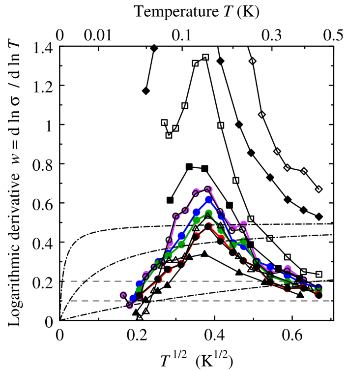
Figure 17: (Color online) Temperature dependences of the logarithmic derivative of the conductivity, $w$, for light-controlled transport in crystalline Cd_0.95Mn_0.05Te_0.97Se_0.03:In studied in Ref. Glod.etal.93, . The presented $w(T)$ data were obtained from the $\sigma(T)$ data published in Ref. Glod.etal.93, as described in the text. Here, we use the same geometric symbols as in the original $\sigma(T)$ plots: All colored symbols relate to data from Figure 1 of Ref. Glod.etal.93, , which reports on measurements of one sample after different illumination times (increasing from top to bottom here); black empty and solid symbols denote data obtained from the $\sigma(T)$ of four samples shown in Figure 2 of Ref. Glod.etal.93, which were measured before and after long illumination, respectively. For comparison, dashed-dotted lines represent $w(T)$ resulting from the hypothetical relation $\sigma=a+b\,T^{1/2}$ with $a/b=0.01$, 0.1, and 1 (from top to bottom). To facilitate judging the slope of the $w(T)$, dashed gray lines mark constant $w=0.2$ and 0.1.

Note, in particular, that all $w(T)$ curves in Figure 17 have negative slope above about 170 mK, even when $w<0.2$. This feature conflicts with the interpretation by Głód et al., who claimed that part of their $\sigma(T)$ originate from metallic transport. These authors, however, left open which of the individual $\sigma(T)$ they considered to indicate metallic transport and which not; in other words, they did not define a specific MIT point. Furthermore, as already stressed above for other disordered solids, this feature is incompatible with the assumption of a continuous MIT with $\sigma$ being proportional to $T^{1/2}$ or $T^{1/3}$ at the transition.

Note, moreover, that all $w(T)$ exhibit clear maxima at roughly the same temperature, at about 140 mK, independently of the respective maximum value of $w(T)$. In this context, we mention the investigation of the light-induced MIT in a related compound semiconductor, crystalline Cd_1-xMn_xTe:In, in Ref. Lei.etal.98, . Examining that study uncovered similar strange behavior of $w(T)$, but in that case at higher temperatures: All $w(T)$ obtained from the data in Ref. Lei.etal.98, exhibit maxima at roughly 0.5 K.Moe.etal.98

Finally, concerning Figure 17, we point to the rapid decrease of all $w(T)$ with decreasing $T$ below about 110 mK, far more rapid than expected according to Eq. (2) with $p=1/2$. Qualitatively, it resembles the rapid decrease of the $w(T)$ curves for Si:P in Figure 8 below about 50 mK. In the case of Cd_0.95Mn_0.05Te_0.97Se_0.03:In, this feature results from the saturation tendency of the individual $\sigma(T)$ below roughly 100 mK apparent in Figures 1 and 2 of Ref. Glod.etal.93, . The authors speculated that this saturation may be related to spin glass freezing, but they seem not to have followed up on this idea in later publications. To us, this feature is more likely due to some experimental artifacts.

4.8 Disordered Gd

We turn now to non-crystalline solids. For several such substances, already more than a decade ago, the augmented power law approach to locating the MIT was shown to fail, see Ref. Moe.Adk, and citations therein. Here, from this group of solids, we first examine the recent investigation of disordered Gd films by Misra et al., Ref. Mis.etal.11, . By means of rf magnetron sputtering, the authors grew thin Gd films on substrates held at 130 K.Mis.etal.11 These films were found to be stable below 77 K. Their sheet resistance could be tuned by annealing at the deposition temperature.Mis.etal.11

Misra et al. evaluated their data by means of a scaling analysis taking for granted continuity of the MIT; they considered the $T$ region from about 5 up to about 50 K. At first glance, their interpretation seems to work nicely, see Figure 3 in Ref. Mis.etal.11, . Several parameters, however, have to be adjusted in that approach, which is always associated with a certain risk of misinterpretation. Therefore, we examine here the justification of the augmented power law fits with adjustable exponents to the measured $\sigma(T)$ data, the first step of that scaling analysis.

In their Figure 2, Misra et al. present a plot of $w(T)$ for a series of samples. It exhibits a $T$-independent separatrix between metallic and insulating samples, a feature which seems to corroborate the assumed continuity of the MIT, compare Figure 20 in our Section 5. This conclusion, however, is not justified for a simple reason: The authors present only the analytical differentiations of their augmented power law fits to $\sigma(T)$ but no numerically differentiated experimental data. Thus, concerning the continuity of the MIT, first and foremost, Misra et al. only got out what they put into their data analysis.

Our Figure 18 compares $w(T)$ relations resulting from the numerical differentiation of the original data with estimates obtained by the analytical differentiation of augmented power law fits. In the former approach, it was non-trivial to find a good compromise between two contradictory demands on the window width: On the one hand, the window shifted along the $\ln\sigma(\ln T)$ curves has to be sufficiently wide to damp the random fluctuations; on the other hand, it has to be kept sufficiently small so that not too much of the low-$T$ part of $w(T)$ is lost. Therefore, we use here a window of variable width: At low $T$, we consider the first two data points, then the first three points, and so on until the $\ln T$ window reaches the width 0.3; after this, we hold the width constant and shift the window along the curve. This approach is not ideal, but it seems to be the best one can do in this case. Certainly, it might overvalue random fluctuations at low $T$.

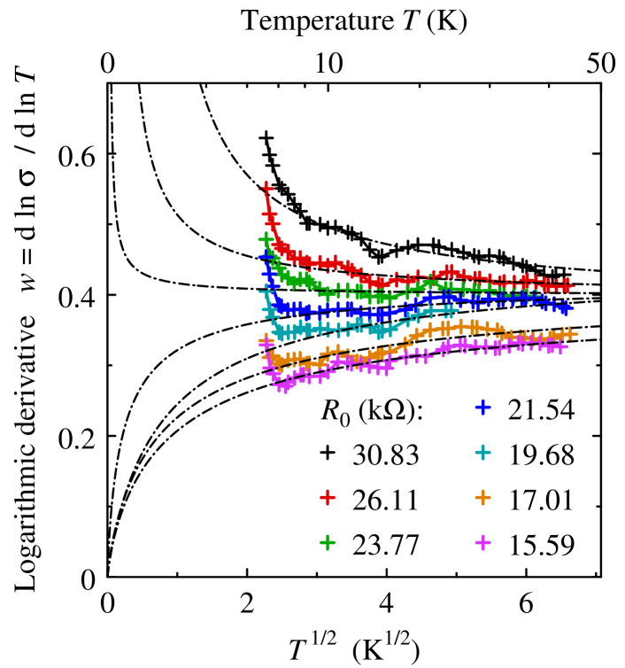
Figure 18: (Color online) Temperature dependences of the logarithmic derivative of the conductivity, $w$, for seven samples of disordered Gd investigated in Ref. Mis.etal.11, . For this reanalysis, we digitized a part of the data sets published in Figure 1 of Ref. Mis.etal.11, , displaying $T$ dependences of the normalized conductivity $\sigma_{\rm n}$. The samples are labeled by their sheet resistance at 5 K, $R_{0}$. We obtained the values of $w(T)$ in two ways: Crosses mark results of numerical differentiation obtained sliding a window of variable width along the $\ln\sigma_{\rm n}(\ln T)$ curves, for details see text; dashed-dotted lines result from analytical differentiation of augmented power law fits with freely adjustable exponents to the experimental $\sigma_{\rm n}(T;R_{0})$ above 8 K.

At about 8 K, our Figure 18 shows a qualitative change in the behavior of the $w(T)$ curves obtained by numerical differentiation. Below this threshold, they exhibit pronounced upturn-like deviations from the analytically differentiated augmented power law fits to the $\sigma(T)$ data points between 8 and about 50 K. Remarkably, these upturns have qualitatively the same shape for all the samples considered here, independently of $R_{0}$, the sheet resistance at 5 K, and independently of whether $w(T)$ decreases of increases with $T$ above 10 K. Hence, it is unlikely that they occur only by chance.

We stress that these upturns are not only present in the $w(T)$ of the samples with $R_{0}\geq 23.77\ \rm{k\Omega}$, classified as insulating in Ref. Mis.etal.11, , but also in the $w(T)$ of the samples with $R_{0}\leq 21.54\ \rm{k\Omega}$, considered as metallic therein. Because this feature is not compatible with the hypothetically metallic $\sigma(T)$ being described by an augmented power law, its presence questions the sample classification in Ref. Mis.etal.11, .

The amplitude of the upturns decreases with $R_{0}$. This might be related to the onset of this feature being shifted to lower $T$ with decreasing $R_{0}$. To some extent, this finding resembles results for insulating samples of amorphous Si_1-xNi_x; in that case, the $w(T,x={\rm const.})$ exhibit pronounced upturns which are shifted to lower $T$ with increasing $x$, see Figure 7 of Ref. Moe.etal.99, . Compare also Figures 3 and 13 in our review, regarding GeSb₂Te₄ and CdSe:In, respectively.

Anyway, the presented comparison of both approaches to obtaining $w(T)$ shows that the interpretation in Ref. Mis.etal.11, is not conclusive. More precise measurements taking into account also moderately lower temperatures are required to reach convincing results.

4.9 Nanogranular Pt-C

As further recent examples of studies on non-crystalline systems, we consider now the investigations of the MIT vicinity of nanogranular W-C and Pt-C published in Refs. Huth.etal.09, and Sac.etal.11, , respectively. These experiments investigated the electrical transport in mesoscopic samples of granular films which were produced by focused electron beam induced deposition of a metal-organic precursor and, in the case of Pt-C, subsequent electron beam irradiation. Due to the very small size of the samples, precise such electrical measurements are demanding.

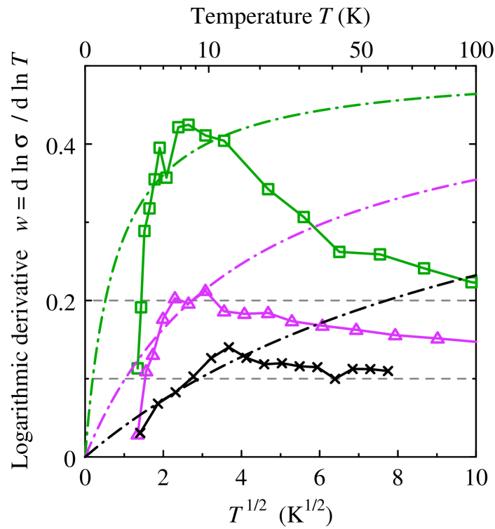
Figure 19: (Color online) Comparison of temperature dependences of the logarithmic derivative of the conductivity, $w$, obtained in two different ways for three nanogranular Pt-C samples from Ref. Sac.etal.11, . These samples were prepared by focused electron beam induced deposition and subsequent electron beam irradiation. Data points marked by green squares and magenta triangles are redrawn from Figure 1b of Ref. Sac.etal.11, . They result from numerical differentiation of the measured $\sigma(T)$ values and refer to two samples irradiated with doses of 0.48 and $0.64\ {\rm\mu C/\mu m^{2}}$, respectively. In addition, data for a sample irradiated with $0.80\ {\rm\mu C/\mu m^{2}}$ are included, labeled by black crosses. They were obtained by digitizing Figure 2a of Ref. Sac.etal.11, and subsequent numerical differentiation, in which pairs of neighboring $\ln\sigma(\ln T)$ points were considered. The dashed-dotted curves, relating to the same measurements of the three samples, were determined by analytical differentiation of the $\sigma=a+b\,T^{1/2}$ fits presented in Figure 2a of Ref. Sac.etal.11, . The dashed gray lines mark marks constant $w=0.1$ and 0.2.

For six W-based granular films, Figure 5 of Ref. Huth.etal.09, shows $w(T^{1/2})$ data obtained by numerical differentiation. Its inset compares these data with analytically differentiated augmented power law approximations for three of the samples. Two problems are obvious here: Below roughly 30 K, $w$ depends on the W content in a nonsystematic manner. Furthermore, the curves obtained by numerical differentiation of the measured data and by analytical differentiation of the augmented power law approximations, respectively, deviate considerably from each other in this $T$ region.

The latter problem is even more striking in the study of Pt-C, Ref. Sac.etal.11, , as we will show now. According to Figure 2a of this publication, $\sigma=a+b\,T^{1/2}$ fits seem to well approximate the measured data between about 1.5 and about 20 K. To check this conclusion, our Figure 19 compares data obtained by numerical differentiation of $\ln\sigma(\ln T)$ with analytic differentiations of $\sigma=a+b\,T^{1/2}$ approximations for three of the investigated samples. We interpret it as follows.

For the two samples labeled by squares and triangles, which were irradiated with doses of 0.48 and $0.64\ {\rm\mu C/\mu m^{2}}$, respectively, the results of both approaches clearly contradict each other: The numerical differentiation yields $w(T)$ increasing with decreasing $T$ down to roughly 8 K and then rapidly decreasing below this temperature. These data suggest that $w(T)$ may either vanish proportionally to a high power of $T^{1/2}$ as $T\rightarrow 0$ or reach 0 already between 1 and 2 K.rem_gr_pt – Note the resemblance to our Figure 8 on Si:P, in particular to the behavior of the colored curves below 50 mK therein, as well as to our Figure 17 regarding persistent photoconductivity in Cd_0.95Mn_0.05Te_0.97Se_0.03:In. – On the contrary, the analytically differentiated augmented power law approximations decrease monotonically with $T$ everywhere and reach 0 only at $T=0$. The sample labeled by crosses, which was irradiated with a dose of $0.80\ {\rm\mu C/\mu m^{2}}$, exhibits similar behavior of $w(T)$ but less pronounced.

Thus, the $w(T)$ obtained by analytical differentiation of $\sigma=a+b\,T^{1/2}$ fits to measured $\sigma(T)$ substantially differ from the results of numerical differentiations not only above 10 K but also below 4 K. Hence, the goodness of the fits shown in Figure 2a of Ref. Sac.etal.11, arises only from the restriction to the transition region between two qualitatively different regimes which both cannot be described by $\sigma=a+b\,T^{1/2}$. We remark that this interpretation is already suggested by careful inspection of the $\sigma$ versus $T^{1/2}$ plots for 0.80 and $1.28{\rm\mu C/\mu m^{2}}$ in Figure 2a of Ref. Sac.etal.11, .

The discrepancies uncovered here may be overlooked on first reading of Ref. Sac.etal.11, for two strange reasons: (i) For the sample irradiated with a dose of $0.64\ {\rm\mu C/\mu m^{2}}$, Figure 2a of Ref. Sac.etal.11, does not include any $\sigma(T)$ points below 4 K, whereas Figure 1b thereof presents $w(T)$ data for this sample down to 2.3 K. (ii) For the sample obtained by irradiation with a dose of $0.48\ {\rm\mu C/\mu m^{2}}$, the $w(T)$ data in Figure 1b of Ref. Sac.etal.11, are not consistent with the $\sigma(T)$ values given in Figure 2a thereof: If these $w(T)$ data are correct, then the $\sigma$ versus $T^{1/2}$ plot must exhibit a saturation tail at low $T$ as it is present in Figure 2a of Ref. Sac.etal.11, for the two samples irradiated with doses of 0.80 and $1.28\ {\rm\mu C/\mu m^{2}}$, respectively, but it does not.

In this way, the comparison presented in our Figure 19 disproves one of the central conclusions drawn in Ref. Sac.etal.11, by Sachser et al.: It is not justified to claim the presence of a universal $T^{1/2}$ contribution to $\sigma(T)$ at low temperatures as the authors did.

4.10 Common features of all $w(T,x)$ diagrams

Concluding this part of our review, we highlight the destructive result common to all the examinations of various experiments from the literature presented in the current section: For none of the samples with $w>0.1$, the behavior of $w(T)$ can be understood in terms of a metallic conduction mechanism which causes $\sigma(T)$ to obey an augmented power law, Eq. (2), with $p=1/2$ or 1/3 over a wide $T$ range.

Simultaneously, we emphasize the constructive result of these analyses: In all examined experiments, there is a wide $T$ range within which the following correlation exists. The logarithmic derivative $w(T)$ seems to always increase with decreasing $T$ when $w>0.1$, that means not only when $w>1/2$, as for (almost) exponential $\sigma(T)$, but also even when $0.1<w\leq 1/2$ arising from comparably weak $T$ dependences of $\sigma$. Only one ⁷⁰Ge:Ga sample with $w\approx 0.25$ considered in Subsection 4.4 might form a slight exception; on broad average, $w(T)$ is roughly constant in this case.

This correlation conflicts with the classification into metallic and insulating samples according to augmented power law extrapolations to $T=0$ used in most of the studies examined here. Furthermore, since, at fixed $T$, $w$ seems to decrease monotonically when the MIT is approached from the insulating side, for example with increasing dopant concentration, this correlation is incompatible with the idea of continuous MIT at which $\sigma\propto T^{p}$ with $p>0.1$.

Additionally, in some but not all studies, our examinations have uncovered a qualitatively different behavior at the lower end of the $T$ range investigated: Here, $w(T)$ decreases with $T$ and vanishes far more rapidly than proportionally to $T^{1/2}$. At the crossover between both scenarios, these $w(T)$ exhibit pronounced maxima with the unusual characteristics described in the following two paragraphs.

Concerning the corresponding temperature value, $T_{\rm max}$, we emphasize two findings: On the one hand, in each of the individual experiments, $T_{\rm max}$ seems to be almost independent of the control parameter. On the other hand, for Si:P, $T_{\rm max}$ differs considerably from experiment to experiment, see Subsection 4.2.

Concerning the peak value of $w(T,x={\rm const.})$, note the following: For Si:P and Cd_0.95Mn_0.05Te_0.97Se_0.03:In, such extrema were found even in the region $w\gtrsim 1$, that means for apparently clearly insulating samples, see Subsections 4.2 and 4.7, respectively.

Together, the findings described in the previous two paragraphs give rise to serious doubts about the soundness of the maxima and thus of the very rapid decreases of $w(T)$ with decreasing $T$ below $T_{\rm max}$.

Because of the observations listed above, none of the experimental studies analyzed here can be considered as conclusive support for a continuous MIT. Instead, as we will show in Section 5, contrasting flow diagrams of $w(T,x={\rm const.})$ obtained from four qualitatively different phenomenological models for the dependence of $\sigma$ on $T$ and control parameter $x$ with the “high-temperature” parts of our Figures 4, 8, 9, 10, 13, 17, and 19 favors the opposite interpretation: This comparison supports the hypothesis that $\lim_{T\rightarrow 0}\sigma(T,x)$ exhibits a discontinuity at the MIT. Nevertheless, since the experimental data are not completely consistent, further and more precise measurements are encouraged.

5 Four possible scenarios of $w(T,x)$

In the previous two sections, considering various solids, we have presented numerous diagrams of $T$ dependences of the logarithmic derivative of the conductivity, $w(T,x={\rm const.})$, which were obtained by numerical differentiation of experimental data from the literature. In most cases, independently of the nature of the control parameter, $x$, these results strikingly conflict with the interpretation in the respective publication.

However, as summarized in Subsection 4.10, our diagrams exhibit obvious similarities with each other. These features are intriguing because, as already pointed to in Subsection 2.6 and Ref. Moe.etal.99, , such plots of $w(T,x={\rm const.})$ for several samples with different values of $x$ can be an informative fingerprint of the character of the MIT.

The direct quantitative evaluation of $w(T,x)$ is hindered by experimental uncertainties and by the necessity of assumptions on $\sigma(T,x)$. Therefore, we here take the opposite approach and analyze the consequences of qualitatively different phenomenological hypotheses: For four very simple phenomenological models describing $\sigma(T,x)$ close to the MIT, we obtain families of $w(T,x={\rm const.})$ curves. In this way, we demonstrate how the character of the MIT determines the qualitative features of such flow diagrams and thus evaluate alternative interpretations of $\sigma(T,x)$ measurements.

First, we assume the MIT occurring at $x_{\rm c}$ to be continuous. That means, we suppose $\sigma(T={\rm const.},x)$ to be continuous there not only at any finite $T$ but also in the limit $T\rightarrow 0$. To construct a simple but sufficiently flexible model of $\sigma(T,x)$ with these characteristics, we start from Eq. (10) of Ref. Moe.etal.99, : We combine modified stretched exponential and augmented power law dependences for the insulating and metallic sides of the MIT, respectively, so that

$$\sigma(T,x)=$$

$$\left\{\begin{array}[]{l}T^{p}\exp(-(T_{0}(x)/T)^{p})\\ \\ a(x)+b(x)\,T^{p}\end{array}\mbox{\ for\ }\begin{array}[]{l}x<x_{\rm c}\\ \\ x\geq x_{\rm c}\end{array},\right.$$ (17)

where $T_{0}(x)$, $a(x)$, and $b(x)$ are continuous functions, and where $T_{0}(x)$ decreases monotonically with $x$, whereas $a(x)$ increases monotonically with $x$. Furthermore, in order to ensure continuity at $x_{\rm c}$, we presume $T_{0}(x\rightarrow x_{\rm c}-0)=0$, $a(x\rightarrow x_{\rm c}+0)=a(x_{\rm c})=0$, and $b(x\rightarrow x_{\rm c}+0)=b(x_{\rm c})=1$. In Eq. (17), for simplicity, all quantities are given in dimensionless form. Moreover, the exponents of the transport mechanisms involved are assumed to have the same value, $p$; certainly, this guess is a gross simplification, but abandoning it would not modify the qualitative features discussed below. – Our continuity and monotonicity presumptions on $T_{0}(x)$, $a(x)$, and $b(x)$ as well as our simplifying assumption on the exponents also apply to the three models considered below. –

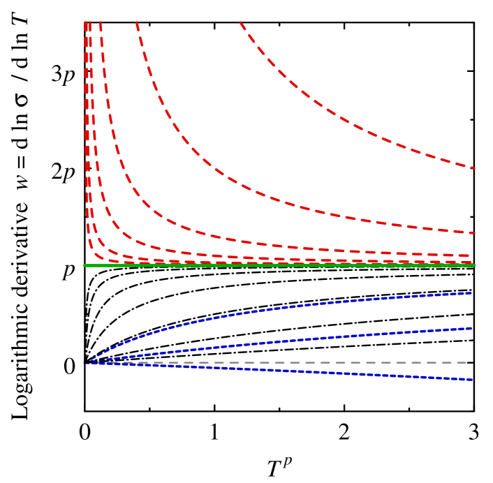
Figure 20: (Color online) Behavior of the logarithmic derivative of the conductivity, $w(T,x={\rm const.})$, for the continuous MIT modeled by Eq. (17). Dashed (red): non-metallic with $T_{0}^{\ p}=3$, 1, 0.3, 0.1, 0.03, and 0.01 (from top to bottom); dashed-dotted (black): metallic with $a=0.01$, 0.03, 0.1, 0.3, 1, 3, 10 and $b\equiv 1$ (from top to bottom); short-dashed (blue): metallic with $a=1$, 3, 10 and $b=1-0.15\,a$ (for smaller values of $a$, such curves would almost coincide with the corresponding relations for $b\equiv 1$); full (green): separatrix, i.e. $w(T,x=x_{\rm c})$. The horizontal dashed gray line marks $w=0$.

Figure 20 shows the flow diagram of $w(T,x={\rm const.})$ for two versions of Eq. (17), $b(x)\equiv 1$ and $b(x)=1-0.15\,a(x)$. In both cases, the regions with metallic and non-metallic behavior do not overlap each other; they are separated by a horizontal line, $w(T,x_{\rm c})=p$. Above this separatrix, that is for non-metallic behavior, the slope, $\mbox{d}w/\mbox{d}T$, is always negative, while, below the separatrix, that is in the metallic region, $\mbox{d}w/\mbox{d}T$ is positive whenever $w>0$; compare Subsection 2.6.

On the metallic side of the MIT, when $b(x)\equiv 1$ as in Eq. (10) of Ref. Moe.etal.99, , our Eq. (17) yields only functions $w(T,x={\rm const.})$ which are positive everywhere except at $T=0$. Hence, for realizing a sign change of $\mbox{d}\sigma/\mbox{d}T$ and thus of $w(T={\rm const.},x)$, the parameter $b$ must depend on the control parameter $x$. In Figure 20, we model such a situation by means of the assumption $b(x)=1-0.15\,a(x)$. (This relation between $a(x)$ and $b(x)$ leads to a good resolution of the family of curves; moderately modifying it does not alter the qualitative features of Figure 20 provided that $b(x_{\rm c})=1$ remains valid.)

One property of this model is particularly noteworthy: The MIT and the sign change of $\mbox{d}\sigma/\mbox{d}T$ occur at different values of $a$ and therefore at different values of $x$; for Eq. (17) with $b(x)=1-0.15\,a(x)$, when $a=0$ and when $a=6.7$, respectively. Hence, according to the model considered here, these phenomena are different in nature, which also follows from the mathematical consideration in Subsection 2.2 by logical contraposition.

Furthermore, just at the MIT described by Eq. (17), $\mbox{d}\sigma/\mbox{d}T=p\,T^{p-1}$. Hence, this derivative is positive at any finite $T$; it diverges as $T\rightarrow 0$ if $p<1$.

Second, for studying how a discontinuous MIT is reflected in the $w(T,x={\rm const.})$ flow diagram, the above model of a continuous MIT has to be modified only slightly. We incorporate an additional constant into the prefactor for the insulating side and change the limiting value of the constant part for the metallic side. Thus we obtain the following generalization of Eq. (11) of Ref. Moe.etal.99, :

$$\sigma(T,x)=$$

$$\left\{\begin{array}[]{l}(1+T^{p})\exp(-(T_{0}(x)/T)^{p})\\ \\ a(x)+b(x)\,T^{p}\end{array}\mbox{\ for\ }\begin{array}[]{l}x<x_{\rm c}\\ \\ x\geq x_{\rm c}\end{array}\right.$$ (24)

with $T_{0}(x\rightarrow x_{\rm c}-0)=0$, $a(x\rightarrow x_{\rm c}+0)=a(x_{\rm c})=1$, and $b(x\rightarrow x_{\rm c}+0)=b(x_{\rm c})=1$. This model exhibits a discontinuity in $\lim_{T\rightarrow 0}\sigma(T,x)$, whereas $\sigma(T={\rm const.},x)$ remains continuous for any $T>0$; compare Figure 11 of Ref. Moe.etal.99, .

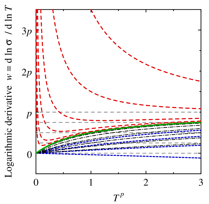
Figure 21: (Color online) Behavior of $w(T,x={\rm const.})$ for the discontinuous MIT modeled by Eq. (24), at which $\mbox{d}\sigma/\mbox{d}T^{p}\,=1$. Dashed (red): non-metallic with $T_{0}^{\ p}=3$, 1, 0.3, 0.1, 0.03, and 0.01 (from top to bottom); dashed-dotted (black): metallic with $a=1.1$, 1.4, 2, 3, 5, 10 and $b\equiv 1$ (from top to bottom); short-dashed (blue): metallic with $a=2$, 3, 5, 10 and $b=1-0.15\,(a-1)$; full (green): separatrix, $w(T,x=x_{\rm c})$. To facilitate judging the slope of the curves, dashed gray lines mark constant $w=0$, $0.25\,p$, $0.5\,p$, $0.75\,p$, and $p$.

Figure 21 presents the flow diagram of $w(T,x={\rm const.})$ for two versions of Eq. (24), that is for $b(x)\equiv 1$ and for $b(x)=1-0.15\,(a(x)-1)$. Again, in both cases, the metallic and non-metallic regions do not overlap each other and, within the metallic region, $w>0$ is correlated with positive slope of $w(T,x={\rm const.})$.

However, in the non-metallic region, $x<x_{\rm c}$, the $w(T,x={\rm const.})$ now have negative slopes for all $x$ values only in the limit $T\rightarrow 0$, in contrast to the curve set in Figure 20. At finite $T$, the sign of the slope varies: Four of the curves exhibit a minimum; it occurs if and only if $T_{0}<1$. The corresponding temperature, $T_{\rm min}(x)$, can take any positive value, whereas $0<w(T_{\rm min},x)<p$.

Note, when the MIT is approached from the insulating side, that means when $T_{0}\rightarrow 0$, both $T_{\rm min}(x)$ and $w(T_{\rm min},x)$ decrease and tend to zero; this can also be easily derived analytically. In consequence, the separatrix $w(T,x=x_{\rm c})$ tends to zero as $T$ vanishes, unlike the separatrix in Figure 20.

Because of the minima in $w(T,x={\rm const.})$, for this model, simultaneously exhibiting positive $w$ and negative slope of $w(T,x={\rm const.})$ at a certain measuring temperature is sufficient but not necessary for a sample to be insulating. Furthermore, the identification of insulating samples is hindered by the following restriction: The closer $x$ to $x_{\rm c}$, the lower the temperatures which have to be considered in order to rule out the possibility of metallic conduction by means of detecting $\mbox{d}w/\mbox{d}T<0$.

As in the case of Eq. (17), the parameter $b$ must depend on $x$ when a sign change of $w(T={\rm const.},x)$ is to be described. In Figure 21, we emulate such a situation assuming $b(x)=1-0.15\,(a(x)-1)$ in analogy to our above consideration of a continuous MIT.

Again, the MIT and the sign change of $\mbox{d}\sigma/\mbox{d}T$, now occurring when $a=1$ and $a=7.7$, respectively, do not coincide. Moreover, as for the model of a continuous MIT considered above, just at the MIT, $\mbox{d}\sigma/\mbox{d}T=p\,T^{p-1}$ is positive at any finite $T$, and diverges as $T\rightarrow 0$ if $p<1$.

Third, the question arises how to construct a model which yields a sign change of $\mbox{d}\sigma/\mbox{d}T$ just at the MIT itself. According to Subsection 2.2, such an MIT must be discontinuous. Thus we start from Eq. (24). Small modifications are sufficient to reach our aim: We only omit the $T$ dependence of the preexponential factor for $x<x_{\rm c},$ appropriately change the limit of $b(x)$, and obtain

$$\sigma(T,x)=$$

$$\left\{\begin{array}[]{l}\exp(-(T_{0}(x)/T)^{p})\\ \\ a(x)+b(x)\,T^{p}\end{array}\mbox{\ for\ }\begin{array}[]{l}x<x_{\rm c}\\ \\ x\geq x_{\rm c}\end{array}\right.$$ (31)

with $T_{0}(x\rightarrow x_{\rm c}-0)=0$, $a(x\rightarrow x_{\rm c}+0)=$ $a(x_{\rm c})=1$, $b(x\neq x_{\rm c})<0$ and $b(x\rightarrow x_{\rm c}+0)=b(x_{\rm c})=0$. This way, the discontinuity of $\lim_{T\rightarrow 0}\sigma(T,x)$ as well as the continuity of $\sigma(T={\rm const.},x)$ for $T>0$ are maintained. Now, for any $T>0$, $\mbox{d}\sigma/\mbox{d}T=0$ holds at and only at $x_{\rm c}$.

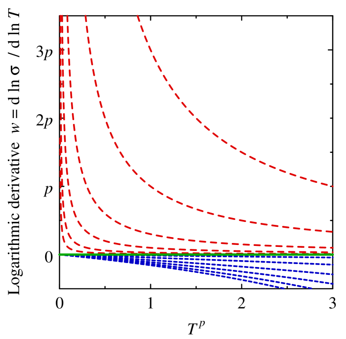
Figure 22: (Color online) Behavior of $w(T,x={\rm const.})$ for the discontinuous MIT modeled by Eq. (31), at which $\mbox{d}\sigma/\mbox{d}T$ changes sign. Dashed (red): non-metallic with $T_{0}^{\ p}=3$, 1, 0.3, 0.1, 0.03, and 0.01 (from top to bottom); short-dashed (blue): metallic with $a=1.1$, 1.4, 2, 3, 5, 10 and $b=-0.15\,(a-1)$ (from top to bottom); full (green): separatrix, $w(T,x=x_{\rm c})$.

The flow diagram of $w(T,x={\rm const.})$ for this model is given in Figure 22, where $b(x)=-0.15\,(a(x)-1)$ is assumed in analogy to the cases previously considered. Again, as in Figure 20 illustrating Eq. (17), non-metallic and metallic regions are separated by a horizontal line, but here by $w(T,x_{\rm c})=0$. Within the metallic region, in contrast to Figure 20, $w(T,x)$ is now negative for any $x>x_{\rm c}$ and any $T>0$. Furthermore, we point out that, in Figure 22, the slope $\mbox{d}w/\mbox{d}T$ is always negative on both sides of the MIT.

One specific feature of Eq. (31) has to be stressed: On the insulating side of the MIT, the $T$ dependences of $\sigma$ can be scaled according to Eq. (5). As discussed in Appendix B, this universality implies that, at the MIT, for any $T>0$, $\mbox{d}\sigma/\mbox{d}T=0$, so that $\mbox{d}w/\mbox{d}T=0$; in the present case, this follows also directly from Eq. (31) and is confirmed by Figure 22.

Fourth, in experiments, however, this inference on $\mbox{d}\sigma/\mbox{d}T$ may only be valid as low-temperature approximation, see Subsections 2.1 and 2.6. Therefore, we now incorporate into Eq. (31) the influence of an additional high-temperature conduction mechanism which enlarges $\sigma(T,x)$ on both sides of the MIT, the more, the higher $T$. To that end, we follow the data analysis approach of a multiplicative decomposition of $\sigma(T)$ in the hopping region proposed in Ref. Moe.etal.85, and extrapolate the contribution of the high-temperature mechanism from the non-metallic into the metallic region similarly as in Ref. Moe.90b, . This results in

$$\sigma(T,x)=$$

$$\left\{\begin{array}[]{l}(1+h(T))\exp(-(T_{0}(x)/T)^{p})\\ \\ a(x)+b(x)\,T^{p}+h(T)\end{array}\mbox{\ for\ }\begin{array}[]{l}x<x_{\rm c}\\ \\ x\geq x_{\rm c}\end{array}\right.$$ (38)

with $T_{0}(x)$, $a(x)$, and $b(x)$ fulfilling the same conditions as for Eq. (31). In line with Ref. Moe.90b, , we assume the high-temperature contribution, $h(T)$, to be independent of $x$. Furthermore, in order to keep the low-temperature behavior described by Eq. (31), we demand that $h(T)/T^{p}\rightarrow 0$ as $T\rightarrow 0$. Under this condition, the qualitative influence of $h(T)$ on the flow diagram of $w(T,x={\rm const.})$ does not depend on the specific form of $h(T)$. As an example, we consider here $h(T)=0.01\,T^{4p}$, describing a quadratic $T$ dependence in case $p=1/2$.

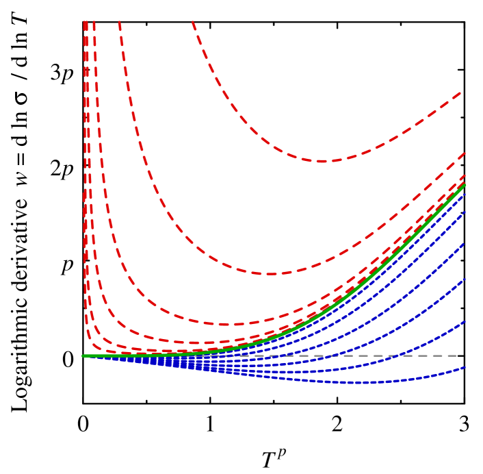
Figure 23: (Color online) Behavior of $w(T,x={\rm const.})$ for a discontinuous MIT which is superimposed by a high-$T$ mechanism contributing to the electrical conduction on both sides of the MIT. This transition is modeled by Eq. (38) with $h(T)=0.01\,T^{4p}$. Here, just at the MIT, $\mbox{d}\sigma/\mbox{d}T=0$ holds only in the limit as $T\rightarrow 0$. For the meaning of the dashed red, short-dashed blue, and full green lines see caption of Figure 22. The dashed gray line indicates $w=0$.

The flow diagram of $w(T,x={\rm const.})$ for Eq. (38) with $b(x)=-0.15\,(a(x)-1)$ is shown in Figure 23. It resembles Figure 21, which illustrates Eq. (24), in two aspects: On the insulating side of the MIT, there are minima, but now in all curves. Furthermore, the separatrix, $w(T,x_{\rm c})$, is $T$-dependent and, again, tends to zero as $T\rightarrow 0$.

In the present case, however, $w(T,x_{\rm c})$ vanishes as $T\rightarrow 0$ far more rapidly than in Figure 21 obtained from Eq. (24). For the immediate vicinity of the MIT, more precisely, for $T_{0}^{p}\ll 0.3$ and $T_{\rm lea}<1$, this difference has important consequences: When curves relating to the same value of $T_{0}$ are compared, the minimum of $w(T,x={\rm const.})$ is reached in Figure 23 at a considerably higher temperature than in Figure 21. Therefore, the width of the $x$ interval within which $w(T,x={\rm const.})$ exhibits positive slope at given $T_{\rm lea}$ despite $x<x_{\rm c}$ is far smaller for Eq. (38) than it is for Eq. (24). Furthermore, at $T_{\rm lea}$, the smallest positive value of $w$ which is correlated with negative $\mbox{d}w/\mbox{d}T$ is now far smaller as well. For these reasons, Eq. (38) may be considered to be more “experimentalist-friendly” than Eq. (24).

On the metallic side of the MIT, two new features arise from the high-temperature contribution $h(T)$: With increasing $T$, all these $w(T,x={\rm const.})$ first pass through a minimum and then change sign at some larger $T$ value. The latter feature indicates the existence of minima in $\sigma(T,x={\rm const.})$ as they have been observed in experiments on crystalline n-Ge:(As,Ga) and Si:As as well as on amorphous Si_1-xCr_x and Si_1-xNi_x; we refer here to Figure 1 of Ref. Zabr.Zino, , Figure 4a of Ref. Koo.Cas.90, , Figure 7 of Ref. Moe.etal.85, , and Figure 8a of Ref. Moe.etal.99, , respectively. The corresponding $T$ values are the lower the closer $x$ to $x_{\rm c}$, see Ref. Moe.etal.85, .

Finally, we highlight a noteworthy relation between the flow diagrams presented in this section: Qualitatively, Figures 21 and 22 can be understood as resulting from Figure 23 by zooming the $T$ scale out or in, respectively.

In the current section, we have presented four simple phenomenological models of $\sigma(T,x)$ close to the MIT yielding flow diagrams of $w(T,x={\rm const.})$ which qualitatively differ from each other. The comparison of experimental graphs to these diagrams can be very helpful in evaluating different hypotheses on the MIT: Note the qualitative similarities between our Figures 4 and 10, on the one hand, and our Figure 22, on the other hand, as well as the resemblance of Figure 13 of the present work and Figure 7 of Ref. Moe.Adk, to our Figure 23. All these similarities support the hypothesis of a discontinuous MIT. Note, furthermore, the qualitative differences between our Figures 4, 10, and 13, on the one hand, and Figure 20, on the other hand. These discrepancies disprove the phenomenological model of a continuous MIT considered here, Eq. (17), for any value of $p$ above 0.1.

6 Summarizing discussion

6.1 Analysis of the available MIT criteria

In the present work, motivated by the recent, seemingly very surprising publication on phase-change materials Ref. Sie.etal.11, , we have examined and critically reviewed the measurement interpretations in numerous experimental studies of the MIT in disordered solids. To find out whether or not the results of Ref. Sie.etal.11, are striking indeed, we started in Section 2 with elucidating the fundamentals of the corresponding data analyses. For this aim, we discussed in detail the available approaches to locate the MIT, that means to discriminate between metallic and insulating samples. In doing so, we showed that making this decision is by far not as simple as it might seem at first glance: Our investigation highlighted substantial biases inherent to the diverse available methods. Although these biases predetermine the result on the character of the MIT to a large extent, their influence has been overlooked in many publications. The related problems are summarized in the following paragraphs.

The MIT in disordered solids is primarily a zero-temperature phenomenon. Therefore, in contrast to early studies as well as to the recent Ref. Sie.etal.11, , conclusions concerning this matter can be drawn only by means of $T\rightarrow 0$ extrapolations. As an approximate substitute, the value of some physical observable at the lowest measuring temperature may be identified with its value at $T=0$. Such an approximation, however, seems to be meaningful only if the considered observable changes sign at the MIT and if, simultaneously, the corresponding control parameter value is sufficiently weakly $T$-dependent.

In this sense, the empirical criterion “sign change of $\mbox{d}\rho/\mbox{d}T$ at the lowest experimentally accessible temperature” has often been used in the literature. However, too little attention has been paid to the point that the supposed validity of this criterion necessarily implies that $\lim_{T\rightarrow 0}\sigma(T,x)$ is a discontinuous function of the control parameter $x$ and jumps from zero to some finite value at the MIT. In a number of cases, this conductivity value was found to roughly equal Mott’s estimate of the hypothetical minimum metallic conductivity. However, as shown in Appendix A, such a correlation is natural already for dimensional reasons.

Consequently, as long as claiming all samples with negative $\mbox{d}\rho/\mbox{d}T$ to be insulating is only an assumption in the data analysis, this correlation alone must not be considered a confirmation of Mott’s theory. Thus, the criterion “sign change of $\mbox{d}\rho/\mbox{d}T$ at the lowest experimentally accessible temperature” exhibits a substantial interpretation bias toward a discontinuous MIT with a finite minimum metallic conductivity.

We stress that this criterion seems to be incompatible with the currently available microscopic theories: First, since it implies the existence of a finite minimum metallic conductivity, it conflicts with all the theories which yield continuity of the MIT, in particular with the scaling theory of localization. Second, since it presumes $\mbox{d}\sigma/\mbox{d}T=0$ to hold just at the MIT, it is incompatible with the idea of an Anderson transition, occurring when the Fermi energy crosses a mobility edge. The latter interpretation, however, neglects electron-electron interaction. Therefore, this discrepancy is not a valid disproof of the hypothesis that, in the limit $T\rightarrow 0$, the MIT is connected with $\mbox{d}\rho/\mbox{d}T$ changing sign.

An alternative approach which has been frequently applied for the last three decades tries to find out when the metallic region is left while the control parameter is varied. In this case, the breakdown of the augmented power law approximation of $\sigma(T)$ is taken as MIT criterion. However, the usual restriction of the breakdown identification to only ask whether or not the adjusted parameter values are physically meaningful implies a substantial analysis bias. The reason is that the possibility of an approximation breakdown indicated by small but systematic deviations between measured data and adjusted function is ignored this way.

In a similar manner, $\sigma(T)$ ceasing to be describable by a stretched Arrhenius law may be interpreted as indication of leaving the insulating region. Such a parameter adjustment, however, is not meaningful when the mean hopping energy is smaller than the lowest experimentally accessible temperature. Moreover, this classification method has the drawback that, in these data analyses, samples with very weak $T$ dependences of $\sigma$ are often classified as metallic without further checks.

Thus, both the two approaches based on augmented power law fits and on stretched Arrhenius law fits, respectively, tend to misclassify weakly insulating samples as metallic. In consequence, the continuity of the MIT concluded in such data evaluations may be only an artifact, and not real.

We stress the significance of just these weakly insulating samples, which exhibit merely nonexponential $\sigma(T)$ within the accessible $T$ range. Their reliable discrimination from metallic ones is of central importance to the trusty characterization of the MIT: An incorrect classification of one or of a very few samples can easily change the answer to the question whether $\lim_{T\rightarrow 0}\sigma(T,x)$ is a continuous function of the control parameter $x$ or whether it exhibits a discontinuity at the MIT. Therefore, the mentioned tendency to misinterpret weakly insulating samples as metallic causes an interpretation bias toward continuity of the MIT. Furthermore, in case the MIT were indeed continuous, such a misclassification could considerably modify the obtained value of the critical exponent of $\lim_{T\rightarrow 0}\sigma(T,x)$.

One cannot escape this problem: Since the mean hopping energy very likely continuously tends to zero when the MIT is approached from the insulating side, going to lower and lower temperatures is of limited value in the characterization of the MIT. In each real experiment, there is a control parameter region of finite width in which only nonexponential $\sigma(T)$ can be observed although the corresponding samples are insulating. For this reason, every success in unambiguously classifying a given set of samples which is reached by diminishing the lowest accessible $T$ value is ruined again when the density of the considered values of the control parameter is increased.

In other words: The relevant temperature scale is set by the mean hopping energy. Hence, very likely in each experiment, when continuously varying the control parameter, one passes the MIT at infinitely high temperature, even if the measurements are performed at a few mK.

We remark that related severe experimental difficulties arise also for another reason: The critical exponent of the characteristic temperature seems to be rather large; it was estimated to amount to $2.1\pm 0.1$ for crystalline n-Ge:(As,Ga) and to $3.0\pm 0.4$ for amorphous Si_1-xCr_x, see Refs. Zabr.Zino, and Moe.90b, , respectively. Therefore, we expect that, to reduce the width of the control parameter region within which only nonexponential $\sigma(T)$ can be observed merely by a factor of 2, the lowest measuring temperature has to be diminished at least by a factor of 4, possibly even by one order of magnitude.

In this context, the study of the logarithmic temperature derivative of the conductivity, $w(T)=\mbox{d}\ln\sigma/\mbox{d}\ln T$, has turned out to be very helpful in classifying individual samples: Assume, on the metallic side of the MIT, $\sigma(T,x)$ follows an augmented power law, $\sigma(T,x)=a(x)+b(x)\,T^{p}$. Then, for any metallic sample with negative $\mbox{d}\rho/\mbox{d}T$, corresponding to positive $w$, on the one hand, $w(T)$ tends to zero as $T\rightarrow 0$ and, on the other hand, $w(T)$ cannot exceed $p$. It is particularly important that, in this case, the slope of the logarithmic derivative is positive, $\mbox{d}w/\mbox{d}T>0$. Consequently, under the assumption made, all samples for which, at low $T$, the inequalities $w>0$ and $\mbox{d}w/\mbox{d}T<0$ simultaneously hold must be insulating.

This implication has the big advantage to unambiguously identify also a large part of the weakly insulating samples with nonexponential $\sigma(T)$. It should be noted, however, that it is based on an assumption, although a plausible one: For each metallic sample with $w>0$, the deviation of $\sigma(T)$ from exact augmented power law behavior is expected to be sufficiently small, that means at least so small that ${\mbox{d}}w/{\mbox{d}}T$ retains the positive sign.

Simultaneously, the evaluation of the logarithmic derivative $w$ yields valuable information also on two other points: First, it is very sensitive to experimental inaccuracies which, despite being small, may qualitatively alter the judgement on the nature of conduction of individual samples; see Sections 3 and 4 for several examples. Second, even more importantly, flow diagrams of $w(T)$ for sets of control parameter values enable conclusions about the character of the MIT. Such diagrams for simple phenomenological models of continuous and discontinuous transitions differ substantially from each other; this was demonstrated in some detail in our Section 5. In particular, if the MIT is continuous and $\sigma=a+b\,T^{p}$ holds on its metallic side, then $0<w<p$ implies $\mbox{d}w/\mbox{d}T>0$. Conflicts between this implication and experimental findings turned out to be central to our study.

6.2 The case GeSb₂Te₄

The above summarized analysis of the available data evaluation approaches provided the basis for critically examining the interpretations in various experimental studies of the MIT in our Sections 3 and 4. In the former part, we scrutinized the seemingly surprising conclusions of the recent work by Siegrist et al. on the MIT in phase-change materials, Ref. Sie.etal.11, , which motivated our work. These authors claimed that GeSb₂Te₄ differs from other disordered systems in two features: the character of the MIT and the strong deviation of the critical charge carrier concentration from the Mott criterion estimate. Our reanalysis of data from Ref. Sie.etal.11, in Section 3 disproved both these claims of differences by means of the following two arguments.

First, as demonstrated in Subsection 3.1, the $\sigma(T)$ curves of GeSb₂Te₄ obtained from Ref. Sie.etal.11, resemble data from other disordered solids in the following sense: There are two GeSb₂Te₄ samples for which, between about 5 and 100 K, $\sigma(T)$ can be well approximated by the ansatz $\sigma=a+b\,T^{1/2}$. For one of these samples, the parameter $a$ has a positive value being by a factor of 100 smaller than the minimum metallic conductivity estimate in Ref. Sie.etal.11, , whereas, for the other, $a$ is approximately zero. – For the $T$ range from 0.35 to about 2 K, an analogous finding was reported in a very recent subsequent study of the MIT in GeSb₂Te₄, Ref. Vol.etal.15, , published by three of the authors of Ref. Sie.etal.11, . – In many previous publications of experiments on various disordered solids, such situations were interpreted as indicating continuity of the MIT, where all samples with positive values of $a$ were regarded as metallic. In Ref. Sie.etal.11, , however, Siegrist et al. classified the sample for which $a$ has a small positive value as clearly insulating and concluded the existence of a finite minimum metallic conductivity. The obvious contradiction between both these interpretations supports the sceptical perspective taken in our introduction: Ref. Sie.etal.11, is a notable example of how the choice of the data evaluation method may predetermine the conclusion on the character of the MIT.

Second, the asserted deviation of the critical charge carrier concentration from the Mott criterion value is unfounded since the latter was obtained in Ref. Sie.etal.11, from an unrealistic guess of the effective Bohr radius of the participating states: In Subsection 3.2, several arguments were given for the electronic transport in the insulating region close to the MIT proceeding via deep defect states presumably originating from vacancies instead of via shallow impurity states as presupposed in Ref. Sie.etal.11, . The latter states can only be crucial in high-quality crystalline semiconductors, additionally provided that the cores of host and impurity atoms resemble each other.

In consequence, there is no reason to agree with Siegrist et al. with respect to ascribing an unusual quantum state of matter to GeSb₂Te₄ and related phase-change materials.

Nonetheless, in Subsection 3.1, also the widely-used analysis by means of $\sigma=a+b\,T^{1/2}$ fits was found to be problematic. We checked the validity of this approximation by considering the logarithmic derivative $w(T)$. From this perspective, the GeSb₂Te₄ sample from Ref. Sie.etal.11, which was prepared by annealing at $T_{\rm ann}=\ 175\ {\rm{}^{o}C}$ is particularly puzzling: According to the $\sigma=a+b\,T^{1/2}$ fit, it should be clearly insulating, in agreement with the classification in Ref. Sie.etal.11, . However, although $w>1/2$ within a wide $T$ range reaching down to roughly 10 K, $w(T)$ seems to vanish as $T\rightarrow 0$. Such a behavior may indicate metallic transport with an augmented power law exponent considerably exceeding $1/2$ or, alternatively, a superposition of at least two $T$-dependent mechanisms. Moreover, this behavior of $w(T)$ may originate from thermal decoupling or from sample inhomogeneities. In all these cases, the $\sigma=a+b\,T^{1/2}$ analysis as a whole cannot be trusted.

Thus, the data evaluation by Siegrist et al., the extrapolations of the $\sigma=a+b\,T^{1/2}$ approximations to $T=0$, and the analysis of the low-$T$ behavior of $w(T)$ yield classifications of the samples into insulating and metallic ones which pairwise contradict each other. Therefore, based on the data in Ref. Sie.etal.11, , a precise determination of the transition point between metallic and insulating behavior is impossible. In consequence, in analyzing these data, the answer to the question whether the MIT in GeSb₂Te₄ is continuous or discontinuous depends on the perspective taken.

In part, the contradictions discussed above may originate from specific features of the $\sigma(T)$ data sets which arise from experimental imperfections. This hypothesis is suggested by our comparison of the low-$T$ part of the experimental $w(T)$ curves of the two most insulating GeSb₂Te₄ samples from Ref. Sie.etal.11, with the theoretical expectations for three different mechanisms of activated conduction.

Further, strong support for this hypothesis comes from the results of the subsequent GeSb₂Te₄ study Ref. Vol.etal.15, . In this work, the investigated $T$ range was extended by one order of magnitude down to 0.35 K. However, apparently, the samples were prepared in the same way as in Ref. Sie.etal.11, . According to the measurements in Ref. Vol.etal.15, , also for the samples annealed at 175 and $200\ {\rm{}^{o}C}$, $w(T)$ clearly increases with decreasing $T$ at the lower end of the $T$ range considered; for the latter sample, $w(T)$ has a minimum value of 0.35. Moreover, for $T_{\rm ann}=225\ {\rm{}^{o}C}$, $w(T)$ is roughly constant between 0.6 and 20 K and amounts to 0.14 there, in clear contradiction to the behavior of analytically differentiated hypothetical $\sigma=a+b\,T^{1/2}$. Thus, all these three samples are very likely insulating.

Beyond the classification of the individual samples, these findings contain valuable information on the character of the MIT: Because of the low values taken by $w$, the $w(T)$ for the samples annealed at 200 and $225\ {\rm{}^{o}C}$ clearly conflict with the interpretation in terms of a continuous MIT with $\sigma\propto T^{1/2}$ at the transition, in contrast to the interpretation in Ref. Vol.etal.15, , but in agreement with the results for many other disordered solids in our Section 4.

Nevertheless, Refs. Sie.etal.11, and Vol.etal.15, demonstrated the possibility to fine-tune localization in GeSb₂Te₄ by annealing. In this approach, various preparation parameters, in particular the composition, can be kept constant. Thus, future such experiments with enhanced precision and accuracy of the $\sigma(T)$ measurements will very likely yield further valuable information on the MIT in disordered systems. At the current stage, however, one related question on GeSb₂Te₄ is still completely open: To what extent do percolation effects arising from inhomogeneities on the grain size scale caused by segregation mask the generic behavior of homogeneous disordered solids?

6.3 Comparison with other solids

Naturally, while analyzing the MIT in phase-change materials, we were confronted with the question of how trustworthy the interpretations in publications on the MIT in other disordered solids are. Therefore, in Section 4, we examined a large number of such studies, in particular frequently cited key publications. The results are alarming: The interpretation problems described above are not specific to the reanalyzed GeSb₂Te₄ measurements. Instead, the inspection of $w(T)$ curve sets for further nine different disordered solids uncovered serious inconsistencies of the augmented power law interpretation in all these cases. Our observations concerning this matter are summarized in the following paragraphs.

(a) The evaluation of data for crystalline Si:As from Ref. Shaf.etal.89, lead to an important conclusion: When, at fixed $T$, in consequence of increasing donor concentration $n$, the MIT is approached from the insulating side, the slope of $w(T,n={\rm const.})$ at low $T$ stays negative while $w$ decreases down to $w$ values below 0.1. This is incompatible with the assumption of a continuous MIT at which $\sigma(T)\propto T^{1/2}$ or $\sigma(T)\propto T^{1/3}$, in contrast to the interpretation in the original work, Ref. Shaf.etal.89, .

(b) The MIT in crystalline Si:P was studied in particularly great detail in the literature. Therefore, exemplarily, we here reproduced and extended the augmented power law analysis from Ref. Waf.etal.99, . Our corresponding diagrams demonstrate the considerable ambiguity of such sample classifications: The obtained transition point depends on the $T$ range considered and in particular on the exponent of $T$ assumed; moreover, the optimum exponent value varies substantially with temperature and distance to the MIT. Furthermore, our check of the augmented power law approach showed that the rather wide linear range in the $\sigma$ versus $T^{1/3}$ plot presented in Ref. Waf.etal.99, does not result from convergence to asymptotic behavior, but that it is implied by inflection points of the measured $\sigma(T^{1/3})$. In order to gain deeper insight, we turned to inspecting $w(T)$ and observed the following. Contrary to the case of Si:As, the $w(T)$ of Si:P exhibit maxima, not only for possibly metallic but also for clearly insulating samples. However, because the corresponding temperature, $T_{\rm max}$, seems to be almost independent of the distance to the MIT and because, moreover, its value is experiment-specific, serious doubts about the reliability of the measurements close to and below the respective $T_{\rm max}$ are suggested. Nevertheless, remarkably, in the temperature range between the puzzling maxima and about 0.6 K, a similar behavior is present as in the case of crystalline Si:As: At fixed $T$, while $w$ decreases with increasing P concentration or increasing stress, $\mbox{d}w/\mbox{d}T$ stays negative at least until $w\approx 0.1$. Hence, extrapolations based on $\sigma=a+b\,T^{1/2}$ or $\sigma=a+b\,T^{1/3}$ are not justified, so that the conclusions about the continuity of the MIT in Refs. Tho.etal.83, , Waf.etal.99, , Ros.etal.80, , Ros.etal.83, , and Stu.etal.93, are called into question.

(c) The results on $w(T,n={\rm const.})$ for the p-type semiconductor Si:B, for which the original publications, Refs. Sara.Dai.02, and Dai.etal.91, , present different interpretations, resemble the findings on the n-type semiconductor Si:As to a large extent. Again, continuity of the MIT with $\sigma(T)\propto T^{1/2}$ or $\sigma(T)\propto T^{1/3}$ just at the transition can be excluded.

(d) Also the $w(T,n={\rm const.})$ curves for neutron-transmutation-doped ⁷⁰Ge:Ga obtained from the data in Ref. Wata.etal.98, qualitatively resemble the corresponding results for Si:As. Our inspection of the $w(T,n={\rm const.})$ for ⁷⁰Ge:Ga lead to the conclusion that $\sigma(T)\propto T^{1/2}$ at the MIT can definitely be ruled out, while $\sigma(T)\propto T^{1/3}$ at the MIT, as concluded in Ref. Wata.etal.98, , is very unlikely but not impossible. Improving the precision of the $\sigma(T)$ measurements should enable a final decision on the latter hypothesis.

(e) In contrast to all other experiments examined in Section 4, the publications on crystalline CdSe:In which we considered there, Refs. Zha.etal.90, , Aha.etal.92, , and Zha.Sara.95, , focus merely on allegedly insulating samples. Because, however, these studies of various aspects of the hopping conduction took into account also samples with only rather weak $T$ dependences of $\sigma$, trying to approximate these $\sigma(T,n={\rm const.})$ by augmented power laws is suggested. Indeed, a $\sigma$ versus $T^{1/2}$ plot shows that, when the analysis is restricted to the $T$ range 0.06 – 0.5 K, one of the CdSe:In samples could be regarded as metallic as well; this resembles the situation for GeSb₂Te₄ discussed in Section 3. When, however, a wider $T$ range is considered, a substantial curvature of $\sigma(T^{1/2})$ becomes obvious and questions the $T\rightarrow 0$ extrapolation according to the ansatz $\sigma=a+b\,T^{1/2}$, just as in the case Si:P. Our subsequent inspection of $w(T,n={\rm const.})$ uncovered interesting similarities to three doped elemental semiconductors: Below about 1 K, these curves strongly resemble the corresponding relations for crystalline Si:As, Si:B, and ⁷⁰Ge:Ga; $\mbox{d}w/\mbox{d}T$ is always negative, even if $w\approx 0.2$. On the contrary, for CdSe:In, above about 15 K, $\mbox{d}w/\mbox{d}T$ is always positive, very likely due to a second conduction mechanism substantially contributing to $\sigma(T)$. The temperature value at which, between the two regions, $w(T,n={\rm const.})$ has its minimum decreases as the MIT is approached, similarly as it was previously observed in studies of a-Si_1-xCr_x and a-Si_1-xNi_x; this feature seems to occur in the case of GeSb₂Te₄, too, see Section 3.

(f) As an example of tuning the MIT by applying a magnetic field of variable field strength $H$, we considered the study of the semimagnetic crystalline semiconductor n-Cd_0.95Mn_0.05Se published in Refs. Wojt.etal.86, and Dietl.etal.86, . In this case, our data analysis uncovered significant inconsistencies between the values published, on the one hand, in the almost identical $\sigma$ versus $T^{1/2}$ diagrams in Figures 1a and 6 of Refs. Wojt.etal.86, and Dietl.etal.86, , respectively, and, on the other hand, in the $\log_{10}\rho$ versus $H^{1/2}$ diagram Figure 4 of Ref. Dietl.etal.86, , presenting detailed data on a wider $(T,H)$-range. Thus, substantial doubts about the reliability of the data basis for the theoretical interpretation in these publications arise. Furthermore, our analysis showed that the behavior of the $w(T,H={\rm const.})$ obtained numerically from the data presented in Figure 4 of Ref. Dietl.etal.86, clearly conflicts with the $w(T)$ resulting from hypothetical $\sigma=a+b\,T^{1/2}$: Again, pronounced maxima of $w(T)$ occur for all considered values of $H$ at roughly the same temperature, here at roughly 0.2 K, even if the transport is very likely non-metallic. Moreover, from 0.2 to 0.4 K, $w$ decreases considerably in all cases, even for the largest field, and thus highest conductivity, for which $w$ falls down to about 0.3. Hence, these data cannot be understood in terms of a continuous MIT at which $\sigma\propto T^{1/2}$.

(g) Evaluating the $\sigma(T)$ data from the attempt in Ref. Glod.etal.93, to fine-tune the MIT in the persistent photoconductor crystalline Cd_0.95Mn_0.05Te_0.97Se_0.03:In by illumination, we obtained a set of $w(T)$ curves which qualitatively resemble the results for Si:P: All $w(T)$ exhibit maxima at roughly 0.14 K, although in several cases the behavior of $w(T)$ above 0.14 K seems to indicate clearly exponential character of $\sigma(T)$. Below this temperature, the $w(T)$ decline far more rapidly with decreasing $T$ than expected in consequence of $\sigma=a+b\,T^{1/2}$. Above it, in all cases, $\mbox{d}w/\mbox{d}T$ stays negative at least up to 0.4 K, even if $w$ is only a little larger than 0.1. Hence, the interpretation in Ref. Glod.etal.93, that a part of the $\sigma(T)$ shown therein exhibits metallic behavior seems unfounded.

(h) The annealing-induced MIT in thin films of disordered Gd was studied in Ref. Mis.etal.11, by means of a scaling analysis relying upon $\sigma=a+b\,T^{p}$ approximations with adjusted $p$ and $w(T)$ relations obtained analytically therefrom. However, the $w(T)$ which we obtained by numerical differentiation of the $\sigma(T)$ from Ref. Mis.etal.11, exhibit substantial systematic low-temperature deviations from the analytical differentiation of respective $\sigma=a+b\,T^{p}$ approximations. Thus, our observation questions the basic assumptions of that work and, in consequence, the validity of the scaling analysis therein.

(i) Finally, for nanogranular Pt-C studied in Ref. Sac.etal.11, , the numerically obtained $w(T)$ data (partially from Ref. Sac.etal.11, ) clearly conflict with $w(T)$ curves which we derived analytically from the $\sigma=a+b\,T^{1/2}$ fits therein: Again, all numerically obtained $w(T)$ have maxima at about the same $T_{\rm max}$. Below $T_{\rm max}$, they decrease far more rapidly with $T$ than expected according to $\sigma=a+b\,T^{1/2}$; above $T_{\rm max}$, the slopes of numerically and analytically obtained $w(T)$ have opposite signs. These findings disprove one of the main results of Ref. Sac.etal.11, , that is the presence of a $T^{1/2}$ contribution to $\sigma(T)$ at low $T$. Furthermore, it is noteworthy that, concerning important low-$T$ details, Figures 1b and 2a of Ref. Sac.etal.11, presenting $w$ versus $T^{1/2}$ and normalized $\sigma$ versus $T^{1/2}$, respectively, are clearly not consistent with each other.

6.4 Conclusions

As a whole, our reanalyses in Sections 3 and 4 provide overwhelming evidence against the usual, localization theory motivated interpretations of the conductivity data in terms of a continuous MIT with $\sigma(T)\propto T^{p}$ and $p=1/2$ or $1/3$ at the transition.

Let us leave aside for a moment the experiment-dependent part of the inconsistencies between augmented power law approximations of $\sigma(T)$ on the one hand and numerically derived $w(T)$ curve sets on the other hand, that is the $T$ region below and close to the puzzling maxima of $w(T)$. Then one feature is common to most of the $w(T)$ sets which we obtained in examining numerous studies on various disordered solids in Section 4: When approaching the MIT at fixed $T$ from the insulating side, while $\mbox{d}w/\mbox{d}T$ stays negative, $w$ decreases down to $w$ values below 0.2, in the cases of Si:As, Si:P, and Si:B even down to $w$ values below 0.1. Because of its apparent universality, this feature cannot be explained in terms of sample-specific inhomogeneities. Thus, it conflicts with all existing and future theories which yield continuity of the MIT and $\sigma(T)\propto T^{p}$ with $p>0.1$ at the transition itself.

The following possibilities remain: (i) Even at the lowest $T$ considered, several mechanisms might superimpose each other, for all disordered solids considered in similar ways. (ii) The MIT might be continuous but with the exponent $p$ being very small, $p<0.1$. (iii) The MIT might be discontinuous, so that the minimum metallic conductivity would be finite.

To us, the discontinuity hypothesis (iii) seems to have the greatest likelihood to be valid for two reasons. First, it is supported by the comparison of the $w(T)$ flow diagrams obtained from experiments on many solids in Section 4 with the results for the phenomenological models considered in Section 5. According to this comparison, the MIT seems to be indicated by $\mbox{d}\sigma/\mbox{d}T$ changing sign at infinitely small $T$. Second, as we discussed in Subsection 2.5, the discontinuity hypothesis is consistent with the scaling of the $T$ dependences of $\sigma$ in the hopping region which had been observed in several MIT studies. As detailed in Appendix B, it is very likely that, even for any $T$ within the temperature validity range of such a scaling relation, the MIT occurs precisely at that control parameter value at which $\mbox{d}\sigma/\mbox{d}T=0$. Nevertheless, at the current stage, because of the experiment-dependent features of $w(T)$ left aside for the moment, we consider our outcome for the character of the MIT still only as speculation, although as a well-founded one.

By questioning the $\sigma(T\rightarrow 0)$ extrapolations based on augmented power laws and thus the resulting sample classifications, our findings also shed new light on the long-standing critical exponent puzzle of the MIT;Hir.etal.88 ; Dai.etal.91 ; Stu.etal.93 see in particular Table I in Ref. Hir.etal.88, . They suggest a surprisingly simple solution: All the different critical exponent values for the control parameter dependence of $\lim_{T\rightarrow 0}\sigma(T)$ in the metallic region which have been reported for various experiments in the literature may not have any physical meaning.

In future experiments, to achieve a compelling phenomenological description of $\sigma(T)$ close to the MIT, the transition has to be considered from different perspectives. In particular, in each such study, consistent $w(T)$ data sets for a series of samples have to be obtained from experiment by numerical differentiation. Because $w(T)$ is very sensitive to small errors of $\sigma(T)$, high precision and accuracy of the measurements are most important. Hence, additionally to ensuring optimum preparation reproducibility and a high degree of sample homogeneity, the following aspects have to be taken care of.

For each individual data point, as in Ref. Moe.etal.99, , the resistance measurement should best be performed only after temperature equilibration has been completed, instead of taking data while $T$ is slowly floating. Since the $\sigma(T)$ curves are only weakly structured, the therefore necessary reduction in the number of data points is not an issue. Furthermore, the linearity of the current-voltage relation has to be carefully checked to eliminate the influence of Joule heating as well as that of non-Ohmic effects. Last but not least, thermal decoupling problems have to be eliminated very thoroughly, even if they are so small that they are almost not noticeable in a conventional plausibility inspection of $\sigma(T)$. For corresponding tests, $w(T)$ data from insulating samples are very useful: They are expected to show systematic control parameter dependence and $\mbox{d}w/\mbox{d}T\leq 0$ down to the lowest measuring $T$. To meet all the listed prerequisites is absolutely necessary for the reliability of experimental investigations of the MIT.

Such a strategy focusing on high-quality $w(T)$ diagrams for sets of samples should enable sensitive checks of the individual data analysis approaches. Thus, it should be very helpful in resolving discrepancies between data evaluations from different perspectives as they have been uncovered in the present work. Only if precision and/or accuracy improvements fail to yield an unambiguous sample classification on the basis of $w(T)$, the intricate extension of the temperature range toward lower $T$ will be indispensable to locate the MIT and to reach a conclusion about its character.

Furthermore, in consequence of the experience gained in our data analyses, we suggest for future experiments to also attach particular importance to the detailed study of the control parameter region where, at the lowest experimentally accessible temperature, $\mbox{d}\sigma/\mbox{d}T$ changes sign. A careful, unbiased analysis of the corresponding weak $T$ dependences of $\sigma$, incorporating samples with positive $\mbox{d}\sigma/\mbox{d}T$ as well as ones with negative $\mbox{d}\sigma/\mbox{d}T$, may be very interesting. It could yield hints whether the hypothesis about the existence of a line of continuous phase transitions in the finite-$T$ part of the $(x,T)$-plane proposed in Subsection 2.5 may have a chance to be true. – If this idea turns out to be true indeed, it will considerably simplify the unambiguous identification of the MIT. – In such an analysis, the relation between the values of $\mbox{d}\sigma/\mbox{d}T$ and of the optimal exponent of a corresponding augmented power law approximation, in which all three parameters are adjusted, may yield valuable information. For a first detailed investigation of this matter see Ref. Moe.90a, , in particular Figure 5 therein. Moreover, searching for a non-analyticity in the relations between the parameters of phenomenological models of $\sigma(T,x={\rm const.})$ which is correlated with $\mbox{d}\sigma/\mbox{d}T=0$ in the low-$T$ limit may be a promising strategy, compare Refs. Moe.etal.85, and Moe.90b, .

The MIT in disordered solids has fascinated physicists for more than fifty years. Nevertheless, for numerous publications of experiments on various such substances, the reanalyses of the reported data from different perspectives in this review have uncovered serious interpretation inconsistencies. According to our comparison with qualitatively different phenomenological models for temperature and control parameter dependences of the conductivity, the hypothesis of a discontinuous MIT occurring precisely when $\mbox{d}\sigma/\mbox{d}T$ changes sign at infinitely small $T$ has a considerably greater likelihood to correctly describe nature than current localization theory claiming continuity of the MIT. It is time to solve this puzzle. For experimentalists, improving the measurement precision should be the most promising strategy. For theoreticians, constructing a microscopic model which is capable to explain the seemingly generic features of the behavior of $\mbox{d}\ln\sigma/\mbox{d}\ln T$ illuminated in this review should be a very rewarding challenge.

APPENDICES

Appendix A Dimensional analysis of relations between characteristic charge carrier concentrations and minimum metallic conductivity

When it is known which input quantities are relevant, dimensional analysis can yield valuable restrictions on the possible outcome of detailed theories. Here, we apply this approach to studying the MIT in heavily doped crystalline semiconductors. In the field of impurity conduction, all theories with the smallest possible material specificity have four dimensioned parameters: the universal constants electron charge, $e$ [A s], and reduced Planck constant, $\hbar$ [kg m² / s], as well as the material parameters effective mass, $m^{*}$ [kg], and permittivity, $\varepsilon$ [(A² s⁴) / (kg m³)].

For determining the critical charge carrier concentration of the MIT, one expresses the edge length of the cube containing one charge carrier, in the following denoted as characteristic length, $l_{\rm c}$ [m], as product of powers of the input parameters,

$$l_{\rm c}=C_{1}e^{\alpha_{1}}\hbar^{\beta_{1}}m^{*\,\gamma_{1}}\varepsilon^{\delta_{1}}\,,$$ (39)

where $C_{1}$ is a dimensionless number. Dimensional analysis yields the following system of equations for the powers of the units kg, m, s, and A.

$$\beta_{1}+\gamma_{1}-\delta_{1}=0$$

$$2\,\beta_{1}-3\,\delta_{1}=1$$

$$\alpha_{1}-\beta_{1}+4\,\delta_{1}=0$$

$$\alpha_{1}+2\,\delta_{1}=0$$

Thus we obtain $\alpha_{1}=-2$, $\beta_{1}=2$, $\gamma_{1}=-1$, and $\delta_{1}=1$ what results in

$$l_{\rm c}=C_{1}\frac{\hbar^{2}\varepsilon}{e^{2}m^{*}}\,.$$ (40)

Since the coefficient matrix of the above system of linear equations is nonsingular, the dimensionless number $C_{1}$ is independent of all dimensioned parameters. Hence, the constant $C_{1}$ is universal, and Eq. (40) describes a proportionality.

Not surprisingly, $l_{\rm c}$ agrees with the effective Bohr radius up to a dimensionless constant. Therefore, for three-dimensional systems, the corresponding critical concentration, $n_{\rm c}=1/l_{\rm c}^{\ 3}$, must satisfy a universal relation with the structure of Eq. (10), where only the constant at the right-hand side remains undetermined.

The condition $\mbox{d}\rho/\mbox{d}T=0$ in the limit as $T\rightarrow 0$ defines a second characteristic length, $\widetilde{l_{\rm c}}$, a corresponding density $\widetilde{n_{\rm c}}$, and a characteristic conductivity value, $\sigma_{\rm c}$. In analogy to Eq. (40), the characteristic length $\widetilde{l_{\rm c}}$ must fulfill the relation

$$\widetilde{l_{\rm c}}=\widetilde{C_{1}}\frac{\hbar^{2}\varepsilon}{e^{2}m^{*}}\,,$$ (41)

where $\widetilde{C_{1}}$ is likewise a universal constant. Therefore, the ratio $\widetilde{l_{\rm c}}/l_{\rm c}$ must be universal and the ratio of the corresponding charge carrier concentrations, $\widetilde{n_{\rm c}}/n_{\rm c}$, as well. According to experiment, the latter quotient should be only slightly larger than 1 in case the MIT is continuous, while, by definition, it is identical to 1 for a discontinuous MIT at which $\mbox{d}\rho/\mbox{d}T$ changes sign in the limit as $T\rightarrow 0$.

Consider now the characteristic conductivity, $\sigma_{\rm c}$. Expressed in SI base units, it is a multiple of (A² s³) / (kg m³) in the three-dimensional case. This quantity, too, must equal a product of powers of the input parameters,

$$\sigma_{\rm c}=C_{2}e^{\alpha_{2}}\hbar^{\beta_{2}}m^{*\,\gamma_{2}}\varepsilon^{\delta_{2}}\,,$$ (42)

where $C_{2}$ is dimensionless. We get the following system of equations for the powers of the units kg, m, s, and A.

$$\beta_{2}+\gamma_{2}-\delta_{2}=-1$$

$$2\,\beta_{2}-3\,\delta_{2}=-3$$

$$\alpha_{2}-\beta_{2}+4\,\delta_{2}=3$$

$$\alpha_{2}+2\,\delta_{2}=2$$

Solving yields $\alpha_{2}=4$, $\beta_{2}=-3$, $\gamma_{2}=1$, and $\delta_{2}=-1$ such that

$$\sigma_{\rm c}=C_{2}\frac{e^{4}m^{*}}{\hbar^{3}\varepsilon}\,.$$ (43)

Since the coefficient matrix of the above system of linear equations is nonsingular, $C_{2}$ is a universal constant, too.

Note that, on the right-hand side of this equation, all the material dependence is contained in the quotient $m^{*}/\varepsilon$. This is also the case on the right-hand side of Eq. (41) determining $\widetilde{l_{\rm c}}$. Therefore, $\sigma_{\rm c}$, $\widetilde{l_{\rm c}}$, and $\widetilde{n_{\rm c}}$ are linked by a universal relation, that is, by

$$\sigma_{\rm c}=\widetilde{C_{1}}C_{2}\frac{e^{2}}{\hbar\widetilde{l_{\rm c}}}=\widetilde{C_{1}}C_{2}\frac{e^{2}}{\hbar}\widetilde{n_{\rm c}}^{1/3}\,.$$ (44)

As a further characteristic conductivity value, the minimum metallic conductivity, $\sigma_{\rm mm}$, be it finite or zero, can be determined in the same way as $\sigma_{\rm c}$. Thus it must be related to the critical charge carrier concentration, $n_{\rm c}$, by an equation of the same form as Eq. (44),

$$\sigma_{\rm mm}=C_{3}\frac{e^{2}}{\hbar l_{\rm c}}=C_{3}\frac{e^{2}}{\hbar}n_{\rm c}^{\ 1/3}\,,$$ (45)

where $C_{3}$ is universal, too. We point out that, up to the dimensionless prefactor, which remains unknown in such a consideration, Eq. (45) agrees with Eq. (1).

In conclusion, considering the three-dimensional case, we have shown that the structures of Eqs. (1) and (10) are robust against various theoretical approximations. In particular, these equations must also result from a theory, which takes electron-electron interaction perfectly into account.

For the two-dimensional case, it can be shown in an analogous manner that $\sigma_{\rm c}$ is a universal quantity being independent of $m^{*}$ and $\varepsilon$.

Appendix B Mathematical aspects of scaling analyses relating $\sigma(T,x={\rm const.})$ data sets of several samples with each other

Suppose we have found that $\sigma(T,x)$ exhibits the following features: (i) For $T\in[T_{\rm lea},T_{\rm utt}]$ and $\sigma\in[\sigma_{\rm a},\sigma_{\rm b}]$, the $\sigma(T,x)$ data of all samples investigated satisfy the scaling relation Eq. (5), repeated here for better readability,

$$\sigma(T,x)=\sigma_{\rm scal}(T/T_{0}(x))\,,$$ (46)

where the control parameter values span the interval $[x_{\rm a},x_{\rm b}]$; in the following, we abbreviate the quotient $T/T_{0}(x)$ by $t$. (ii) At the lower end of $[\sigma_{\rm a},\sigma_{\rm b}]$, $\sigma(T,x={\rm const.})$ decreases exponentially with $T$ according to Eq. (4),

$$\sigma(T,x)=\sigma_{0}(x)\,\exp(-(T_{0}(x)/T)^{\nu})\,.$$ (47)

The validity of the scaling relation Eq. (46) implies that $\sigma_{0}(x)$ is an $x$-independent constant.

As discussed in Subsection 2.5, we infer from (i) and (ii) that $[x_{\rm a},x_{\rm b}]$ belongs to the insulating side of the MIT. Strictly speaking, this conclusion relies on two plausible suppositions: (iii) For $T\in[T_{\rm lea},T_{\rm utt}]$, Eq. (46) is valid for any $x\in[x_{\rm a},x_{\rm b}]$. (iv) $\lim_{T\rightarrow 0}\sigma(T,x)=0$ holds as consequence of (ii) and (iii) for any $x\in[x_{\rm a},x_{\rm b}]$.

In our further analysis, considering the $T$ interval $(0,T_{\rm utt}]$, we rely on three plausible presumptions about the vicinity of the MIT: (v) The conductivity $\sigma(T,x)$ is a continuous function of both $T$ and $x$. (vi) Without loss of generality, for any $T>0$, $\sigma(T={\rm const.},x)$ increases strictly monotonically with $x$. (vii) On the insulating side of the MIT, $\sigma(T,x={\rm const.})$ increases strictly monotonically with $T$ within the scaling domain.

In consequence of (vi), (vii), Eq. (46), and since $\partial\sigma/\partial x=\mbox{d}\sigma_{\rm scal}(t)/\mbox{d}t\ \partial t/\partial x=\mbox{d}\sigma_{\rm scal}(t)/\mbox{d}t\ (-T/T_{0}(x)^{2})\ \mbox{d}T_{0}(x)/\mbox{d}x=\mbox{d}\sigma_{\rm scal}(t)/\mbox{d}t\ (1/T_{0}(x))\ (-T/T_{0}(x))\ \mbox{d}T_{0}(x)/\mbox{d}x=\mbox{d}\sigma_{\rm scal}(t)/\mbox{d}t\ \partial t/\partial T\ (-T/T_{0}(x))\ \mbox{d}T_{0}(x)/\mbox{d}x=\partial\sigma/\partial T\ (-T/T_{0}(x))\ \mbox{d}T_{0}(x)/\mbox{d}x$ so that $\mbox{d}T_{0}(x)/\mbox{d}x=-(T_{0}(x)/T)\ \partial\sigma/\partial x\ \Big{/}\ \partial\sigma/\partial T$, the function $T_{0}(x)$ must decrease strictly monotonically with increasing $x$ and can thus be inverted. Hence, there is a function $x_{0}(T)$ with $x_{0}(T_{0}(x))=x$. Furthermore, because of (vi), the critical control parameter value of the MIT, $x_{\rm c}$, must exceed $x_{\rm b}$.

Now, as key to the physical interpretation, we make a first generalizing hypothesis: (viii) We suppose that the scaling relation Eq. (46) holds whenever $T\in(0,T_{\rm utt}]$, $\sigma\in(0,\sigma_{\rm b}]$, as well as $x\geq x_{\rm a}$ and that $\lim_{t\rightarrow 0}\sigma_{\rm scal}(t)=0$.

The generalizing hypothesis (viii) has two immediate consequences: It excludes metallic conduction within the whole considered scaling domain and thus implies the existence of a finite minimum metallic conductivity, $\sigma_{\rm mm}$, related to $T\in(0,T_{\rm utt}]$, where $\sigma_{\rm mm}\geq\sigma_{\rm b}$. Furthermore, hypothesis (viii) means that, for $x\geq x_{\rm a}$, there is no non-metallic conduction without $\sigma(T,x)$ satisfying Eq. (46) at sufficiently low $T$. Thus, this way, the corresponding control parameter interval is extended beyond $x_{\rm b}$ up to the MIT at $x_{\rm c}$.

We reach an important conclusion on $T_{0}(x)$: Without loss of generality, be $\sigma_{\rm scal}(T/T_{0}(x)=1)=\sigma^{\star}\in[\sigma_{\rm a},\sigma_{\rm b}]$. For $T\in(0,T_{\rm lea}]$, we have $\sigma(T,x_{\rm a})\leq\sigma(T_{\rm lea},x_{\rm a})\leq\sigma_{\rm a}$, whereas, for approaching the MIT at $x_{\rm c}$ from the metallic side, $\sigma(T,x_{\rm c}+0)\geq\sigma_{\rm mm}\geq\sigma_{\rm b}$. Thus, according to (v), (vi), and the intermediate value theorem, for any arbitrarily small $\tilde{T}$, there is one and only one $\tilde{x}$ with $\sigma(\tilde{T},\tilde{x})=\sigma^{\star}$. Since, because of (viii) and the definition of $\sigma^{\star}$, $T_{0}(\tilde{x})$ equals $\tilde{T}$, we conclude that $T_{0}(x)$ can take arbitrarily small values. Therefore, due to $T_{0}(x)$ decreasing strictly monotonically with increasing $x$ and due to the physical condition $T_{0}(x)>0$, the $x$ domain of $\sigma_{\rm scal}(T/T_{0}(x))$ ends at $\lim_{\tilde{T}\rightarrow 0}x_{0}(\tilde{T})$, and so does the validity region of the scaling relation Eq. (46).

This control parameter value marks the MIT, $x_{\rm c}=\lim_{\tilde{T}\rightarrow 0}x_{0}(\tilde{T})$, because, as concluded above, for $x\geq x_{\rm a}$, there is no non-metallic conduction without $\sigma(T,x)$ satisfying Eq. (46) at sufficiently low $T$. In other words, the generalizing hypothesis (viii) together with the continuity and the strict monotonicity of $\sigma(T={\rm const.},x)$ imply $T_{0}(x)\rightarrow 0$ as $x\rightarrow x_{\rm c}-0$. In this sense, under the above suppositions, scaling of the $\sigma(T,x={\rm const.})$ curves for various $x$ answers the question about the limiting behavior of the mean hopping energy, posed in Subsection 2.2.

Up to now, the condition $\sigma(T,x)\leq\sigma_{\rm b}$ restricts the domain of the argument $t=T/T_{0}(x)$ of the scaling function $\sigma_{\rm scal}(t)$ to the finite interval $(0,t_{\rm b}]$ where $t_{\rm b}$ is given by $\sigma_{\rm scal}(t_{\rm b})=\sigma_{\rm b}$. Thus, we are confronted with the following problem: According to experimental experience, close to the MIT, the scaling verification is hindered by the increasingly weak $T$ dependence of $\sigma$ as $x\rightarrow x_{\rm c}$, see, e.g., Figures 4 and 1 of Refs. Moe.etal.83, and Liu.etal.92, , respectively. This is the natural consequence of $T_{\rm utt}/T_{0}(x)$ diverging as $x\rightarrow x_{\rm c}$.

Note, because of this singularity, to verify Eq. (46) by a mastercurve construction also for the region $\{T\leq T_{\rm utt},x<x_{\rm c},\sigma>\sigma_{\rm b}\}$, one would need an infinite number of samples. In consequence, there always is a finite $x$ interval adjacent to the MIT where one cannot reliably verify Eq. (46) by experiment. Since it would seem unphysical, however, that scaling would break down just when $x$ approaches $x_{\rm c}$, we rely on a second generalizing hypothesis: (ix) We suppose Eq. (46) to be valid whenever $T\in(0,T_{\rm utt}]$ and $x\in[x_{\rm a},x_{\rm c})$. Within this domain, $\sigma(T,x)\leq\sigma(T_{\rm utt},x)<\sigma(T_{\rm utt},x_{\rm c})$, so that $\sigma_{\rm c}=\lim_{x\rightarrow x_{\rm c}-0}\sigma(T_{\rm utt},x)=\sigma(T_{\rm utt},x_{\rm c})$ can be interpreted as maximum non-metallic conductivity.

Because of supposition (v), generalizing hypothesis (ix), and $\lim_{x\rightarrow x_{\rm c}-0}T_{0}(x)=0$, we finally obtain that $\sigma(T,x_{\rm c})=\lim_{x\rightarrow x_{\rm c}-0}\sigma(T,x)=\lim_{T_{0}\rightarrow 0}\sigma_{\rm scal}(T/T_{0})=\lim_{t\rightarrow\infty}\sigma_{\rm scal}(t)=\lim_{T_{0}\rightarrow 0}\sigma_{\rm scal}(T_{\rm utt}/T_{0})=\sigma_{\rm c}$ holds for any $T\in(0,T_{\rm utt}]$. – In the insulating region, the limits for $x$ and $T$ do not commute, $\sigma_{\rm c}=\lim_{T\rightarrow 0}\lim_{x\rightarrow x_{\rm c}}\sigma(T,x)\neq\lim_{x\rightarrow x_{\rm c}}\lim_{T\rightarrow 0}\sigma(T,x)=0$. –

Furthermore, we now see that, due to the monotonicity supposition (vi), provided $T\leq T_{\rm utt}$, the relation $\sigma(T,x)<\sigma_{\rm c}$ is satisfied if and only if $x<x_{\rm c}$. Hence, because of the continuity supposition (v), the maximum non-metallic conductivity coincides with the minimum metallic conductivity, $\sigma_{\rm c}=\sigma_{\rm mm}$.

For the MIT itself, $x=x_{\rm c}$, we showed above that $\sigma$ is independent of $T$, $\partial\sigma(T,x_{\rm c})/\partial T=0$. We now ask for the behavior of $\partial\sigma(T,x)/\partial T$ in the insulating vicinity of the MIT: Due to Eq. (46) and suppositions (vii) and (ix), $\sigma_{\rm scal}(t)$ increases monotonically with $t$. Therefore, the finiteness of $\sigma_{\rm c}=\lim_{t\rightarrow\infty}\sigma_{\rm scal}(t)$ implies that $\mbox{d}\sigma_{\rm scal}(t)/\mbox{d}\ln t\rightarrow 0$ as $t\rightarrow\infty$. Because, moreover, $\mbox{d}\sigma_{\rm scal}(t)/\mbox{d}\ln t=\mbox{d}\sigma_{\rm scal}(T/T_{0})/\mbox{d}\ln T=T\mbox{d}\sigma_{\rm scal}(T/T_{0})/\mbox{d}T=T\partial\sigma(T,x)/\partial T$, we thus obtain that, for any $T\in(0,T_{\rm utt}]$, $\partial\sigma(T,x)/\partial T$ continuously tends to zero as $x\rightarrow x_{\rm c}-0$.

This way, the scaling relation Eq. (46) together with a few plausible assumptions imply the condition $\mbox{d}\rho/\mbox{d}T=0$ to mark the MIT and to yield the value of the minimum metallic conductivity. Since scaling according to Eq. (46) is a low-$T$ phenomenon, our mathematical consideration supports the empirical MIT criterion “$\mbox{d}\rho/\mbox{d}T=0$ in the limit as $T\rightarrow 0$”, discussed in detail in Subsection 2.2.

One may now ask, what would happen if any of the above suppositions were violated in some respect, e.g., (v) by a small positive step in $\sigma(T={\rm const.},x)$ at $x_{\rm c}$, whereas, as $x\rightarrow x_{\rm c}-0$, Eq. (46) and the limiting behavior $T_{0}(x)\rightarrow 0$ were maintained for $T\in(0,T_{\rm utt}]$. In this case, the answer is that, together with the monotonicity supposition (vi) on the $x$ dependence of $\sigma$, these relations would be sufficient to imply the existence of a finite minimum metallic conductivity. This can also be easily shown by an indirect proof: Suppose the MIT is continuous and $\lim_{x\rightarrow x_{\rm c}+0}\sigma(T,x_{\rm c})=b\,T^{p}$. Then, for $T<(\sigma_{\rm c}/b)^{1/p}$, we get $\lim_{x\rightarrow x_{\rm c}-0}\sigma(T,x)=\sigma_{\rm c}>\lim_{x\rightarrow x_{\rm c}+0}\sigma(T,x)$ in contradiction to our monotonicity supposition.

The situation would be totally different if $T_{0}$ tended to a finite value as $x\rightarrow x_{\rm c}$. Then $\lim_{x\rightarrow x_{\rm c}-0}\sigma(T,x)$ would be $T$-dependent, in contrast to our conclusion $\lim_{x\rightarrow x_{\rm c}-0}\sigma(T,x)=\sigma_{\rm c}\,={\rm const.}$ drawn above. The limit would fall off exponentially as $T\rightarrow 0$. Therefore, in consequence of the very likely continuity of $\sigma(T={\rm const.},x)$, $\lim_{x\rightarrow x_{\rm c}+0}\sigma(T,x)$ would fall off exponentially as well, so that the MIT would be continuous. – Note that this limiting behavior would be incompatible with the generalizing supposition (viii). – Moreover, just on the metallic side of the MIT, $\sigma(T,x={\rm const.})$ had to follow a stretched Arrhenius law augmented by a small $x$-dependent constant contribution instead of an augmented power law. To the best of our knowledge, however, such a situation has not been reported up to now.

Appendix C Method for numerical differentiation of functions given by noisy values at non-equidistant points

The present study relies to a large extent on the as accurate as possible numerical differentiation of functions given by sets of experimental data points. For explaining our approach to this numerical task, we first remind that uncertainties of derivative values approximated by difference quotients originate both from random errors of the data and from nonlinearities of the considered function. To reduce the influence of random errors, the argument intervals used to calculate the difference quotients should be as wide as possible. However, the wider the interval, the stronger is the influence of nonlinearities. In consequence, there is an optimum interval width; its size depends on which differentiation formula is used.

When not only two, but many data points are taken into account, the corresponding averaging further reduces the influence of their random errors. Thus, we aim to slide a window along the curve and to estimate the local slope by means of linear regression on all data points within the window. In case of equidistant argument values, this can be realized by applying a special Savitzky-Golay filter; in this approach, the slope value is related to the average of the smallest and largest argument values within the window.Sav.Gol

For the present study, however, we need a procedure which is applicable to the general case of non-equidistant arguments. The approach which we use in this work has proved to be very effective in our research for many years; in particular, Eqs. (8) and (9) of Ref. Moe.etal.99, were obtained this way. However, this approach seems to be widely unknown. Therefore, we present here a short derivation in general notation.

The idea of our procedure is the following: In each regression, we additionally determine that argument value for which the linear regression slope is expected to be the best approximation of the derivative. In other words, we ask: For which argument choice do nonlinearities have the smallest influence?

To answer this question, we need an adequate quantification of these deviations. The truncation error, resulting from the truncation of the corresponding Taylor series, is best suited for this aim. We remind here that, in considering difference quotients obtained from two data points with the arguments differing by $h$, the midpoint formula is far superior to forward and backward differentiation formulas. The reason is the following: In the former case, the leading term of the truncation error arising from nonlinearities is proportional to $h^{2}$, while in the latter cases it is proportional to $h$ and thus usually far larger; the random error is always the same and proportional to $h^{-1}$. Therefore, for the midpoint formula, the total error is considerably smaller and the optimum interval width is much wider than for the forward or backward formulas.

Consider now the physical quantities $x$ and $y$ which are linked by the function $y=f(x)$. Assume, we performed $k$ measurements and obtained the data points $(x_{i},y_{i})$, where at least two of the $x_{i}$ values differ from each other. Assume, furthermore, that the uncertainties of the $x_{i}$ are negligible and that the random errors of all $y_{i}$ have the same standard deviation. (The generalization of the approach described here to the case of different standard deviations of the random errors of the individual $y_{i}$ is straightforward.)

In the first step, capturing only lowest-order nonlinearities, we approximate $f(x)$ by the quadratic ansatz

$$\varphi(x)=a+b\,x+c\,x^{2}\,,$$ (48)

where the values of the parameters $a$ and $b$ have to be adjusted, and where, for the moment, we assume that we know the value of $c$.

To determine the values of $a$ and $b$, we minimize the sum of the squared deviations,

$$\sum_{i}(y_{i}-a-b\,x_{i}-c\,{x_{i}}^{2})^{2}\ \rightarrow\ \min\,.$$ (49)

Differentiation with respect to $a$ and $b$ yields the normal equations,

$$a\,k+b\,\sum_{i}x_{i}=\sum_{i}y_{i}-c\,\sum_{i}{x_{i}}^{2}\,,$$ (50)

$$a\,\sum_{i}x_{i}+b\,\sum_{i}{x_{i}}^{2}=\sum_{i}x_{i}\,y_{i}-c\,\sum_{i}{x_{i}}^{3}\,,$$ (51)

so that

$$b=b_{0}+b_{1}\,c$$ (52)

with

$$b_{0}=\frac{k\,\sum_{i}x_{i}\,y_{i}-\sum_{i}x_{i}\,\sum_{j}y_{j}}{k\,\sum_{i}{x_{i}}^{2}-(\sum_{i}x_{i})^{2}}\,,$$ (53)

$$b_{1}=\frac{-k\,\sum_{i}{x_{i}}^{3}+\sum_{i}x_{i}\,\sum_{j}{x_{j}}^{2}}{k\,\sum_{i}{x_{i}}^{2}-(\sum_{i}x_{i})^{2}}\,.$$ (54)

Equation (53) is the well-known result for the slope obtained by linear regression. Finally, combining Eqs. (48) and (52), we get the derivative approximation

$$\frac{\mbox{d}\varphi}{\mbox{d}x}(x)=b_{0}+(b_{1}+2\,x)\,c\,.$$ (55)

Now, the decisive idea is to focus on that $x$ value, $x_{\rm a}$, where we do not need the knowledge of $c$, which we only pretended to have above. The prefactor of $c$ on the right-hand side of Eq. (55) vanishes at

$$x_{\rm a}=-\frac{b_{1}}{2}=\frac{k\,\sum_{i}{x_{i}}^{3}-\sum_{i}x_{i}\,\sum_{j}{x_{j}}^{2}}{2\,(k\,\sum_{i}{x_{i}}^{2}-(\sum_{i}x_{i})^{2})}\,.$$ (56)

Thus, at $x_{\rm a}$, as in the case of the midpoint formula of differentiation, the quadratic contribution to $\varphi(x)$ has no influence on the calculated value of $\mbox{d}\varphi/\mbox{d}x$.

Hence, for any quadratic polynomial $f(x)$, arbitrarily positioned $x_{i}$, and negligible random errors of $y_{i}$, the linear regression slope $b_{0}$ when related to the specific argument average $x_{\rm a}$ exactly equals the derivative value. (In case, the $x_{i}$ are equidistant, $x_{\rm a}$ reduces to the mean value of smallest and largest $x_{i}$ considered, which is in agreement with Ref. Sav.Gol, . For $k=2$, as well as for $k=3$ with equidistant $x_{i}$, our result is identical to the midpoint formula of differentiation.)

In the second step, we consider an arbitrary analytic function $f(x)$, but neglect the random errors of the $y_{i}$. Inserting the Taylor expansion of $f(x)$ about $x_{\rm a}$ into Eq. (53) yields after a short calculation

$$b_{0}=\frac{\mbox{d}f}{\mbox{d}x}(x_{\rm a})\,+$$

$$\frac{1}{6}\,\frac{k\,\sum_{i}{\overline{x}_{i}}^{4}-\sum_{i}\overline{x}_{i}\,\sum_{j}{\overline{x}_{j}}^{3}}{k\,\sum_{i}{\overline{x}_{i}}^{2}-(\sum_{i}\overline{x}_{i})^{2}}\,\frac{\mbox{d}^{3}f}{\mbox{d}x^{3}}(x_{\rm a})\,+$$

$$...\,,$$ (57)

where $\overline{x}_{i}=x_{i}-x_{\rm a}$. Hence, when rescaling all $\overline{x}_{i}$ by a factor $\alpha$, one has to multiply the leading term of the truncation error of $\mbox{d}f/\mbox{d}x(x_{\rm a})$ by the factor $\alpha^{2}$. In this sense, when the number of data points and all quotients of argument differences, $x_{i}-x_{j}$, are kept fixed, the truncation error of the value of $\mbox{d}f/\mbox{d}x(x_{\rm a})$ is proportional to the square of the window width, $(\max\{x_{i}\}-\min\{x_{i}\})^{2}$. Thus, this truncation error is usually far smaller than that of the value of $\mbox{d}f/\mbox{d}x(x)$ for $x\neq x_{\rm a}$, which is proportional to the window width itself. This result corresponds to the properties of the truncation errors of two-point formulas mentioned above.

Therefore, relating to $x_{\rm a}$ often enables the use of quite wide windows including rather large numbers of data points. In this way, the random errors of the derivative values, obtained by numerical differentiation, are usually considerably reduced compared to the random dispersion of values resulting from two-point formulas. – Note, however, that these random errors are always correlated over the window width. – Furthermore, due to the averaging, the prefactor in the truncation error of the derivative value obtained by our approach is usually appreciably smaller than that for the two-point midpoint formula considering the same argument interval. In consequence, a far smaller total uncertainty of the value of $\mbox{d}f/\mbox{d}x$ can be reached by linear regression with relating the slope to $x_{\rm a}$ than by applying common difference quotient approaches.

It is worth mentioning that the influence of the truncation error may be diminished even further. For this aim, $f(x)$ has to be transformed to a function $\phi(\xi)$ with weaker nonlinearity. After calculating $\mbox{d}\phi/\mbox{d}\xi$ by means of the procedure described above, one obtains the $\mbox{d}f/\mbox{d}x$ data using common differentiation rules.

Finally, we would like to emphasize that the presented method is very flexible. We have utilized it in various ways, sliding a window along experimental relations $f(x)$ and obtaining pointwise $\mbox{d}f/\mbox{d}x$ from all $(x_{i},y_{i})$ within the window. As always with numerical differentiation, the art of applying this method consists in the choice of an appropriate window width which ensures a reasonable compromise between conflicting demands: On the one hand, the random errors of the obtained derivative values of $f(x)$ should be as small as possible, while, on the other hand, the truncation errors should not be too large and the essential features of $\mbox{d}f/\mbox{d}x(x)$ must not be smeared out too much.

References

- (1) A. Lagendijk, B. van Tiggelen, and D.S. Wiersma, Fifty years of Anderson localization, Phys. Today 62, 24–29 (2009).
- (2) 50 Years of Anderson Localization, ed. E. Abrahams, World Scientific, Singapore (2010).
- (3) N.F. Mott and E.A. Davis, Electronic Processes in Non-Crystalline Materials, 2nd edition, Clarendon Press, Oxford (1979).
- (4) N.F. Mott, Metal-Insulator Transitions, 2nd edition, Taylor and Francis, London (1990).
- (5) P.A. Lee and T.V. Ramakrishnan, Disordered electronic systems, Rev. Mod. Phys. 57, 287–337 (1985).
- (6) D. Belitz and T.R. Kirkpatrick, The Anderson-Mott transition, Rev. Mod. Phys. 66, 261–380 (1994).
- (7) P.P. Edwards, The metal-nonmetal transition: the continued/unreasonable effectiveness of simple criteria at the transition, in Perspectives in Solid State Chemistry, ed. K.J. Rao, Wiley, New York (1995), pp. 250–271.
- (8) P.P. Edwards, T.V. Ramakrishnan, and C.N.R. Rao, The Metal-Nonmetal Transition: A Global Perspective, J. Phys. Chem. 99, 5228–5239 (1995).
- (9) H. v. Löhneysen, Metal-insulator transition in heavily doped semiconductors, Curr. Opin. Solid State Mater. Sci. 3, 5–15 (1998).
- (10) A. Möbius and C.J. Adkins, Metal-insulator transition in amorphous alloys, Curr. Opin. Solid State Mater. Sci. 4, 303–314 (1999).
- (11) F. Evers and A.D. Mirlin, Anderson transitions, Rev. Mod. Phys. 80, 1355–1417 (2008).
- (12) P.W. Anderson, Absence of diffusion in certain random lattices, Phys. Rev. 109, 1492–1505 (1958).
- (13) N.F. Mott, Conduction in non-crystalline systems IX. The minimum metallic conductivity, Phil. Mag. 26, 1015–1026 (1972).
- (14) E. Abrahams, P.W. Anderson, D.C. Licciardello, and T.V. Ramakrishnan, Scaling theory of localization: Absence of quantum diffusion in two dimensions, Phys. Rev. Lett. 42, 673–676 (1979).
- (15) A.M. Finkel’shteĭn, Influence of Coulomb interactions on the properties of disordered metals, Sov. Phys. JETP 57, 97–108 (1983) [Translation of Zh. Eksp. Teor. Fiz. 84, 168–189 (1983).]
- (16) C. Yamanouchi, K. Mizuguchi, and W. Sasaki, Electric conduction in phosphorus doped silicon at low temperatures, J. Phys. Soc. Jpn. 22, 859–864 (1967).
- (17) A.G. Zabrodskiĭ and K.N. Zinov’eva, Low-temperature conductivity and metal-insulator transition in compensate n-Ge, Sov. Phys. JETP 59, 425–433 (1984) [Translation of Zh. Eksp. Teor. Fiz. 86, 727-742 (1984)].
- (18) W.N. Shafarman, D.W. Koon, and T.G. Castner, dc conductivity of arsenic-doped silicon near the metal-insulator transition, Phys. Rev. B 40, 1216–1231 (1989).
- (19) G. Hertel, D.J. Bishop, E.G. Spencer, J.M. Rowell, and R.C. Dynes, Tunneling and transport measurements at the metal-insulator transition of amorphous Nb:Si, Phys. Rev. Lett. 50, 743–746 (1983).
- (20) A. Möbius, D. Elefant, A. Heinrich, R. Müller, J. Schumann, H. Vinzelberg, and G. Zies, The metal-semiconductor transition in amorphous Si1-xCrx films – scaling behaviour and minimum metallic conductivity, J. Phys. C 16, 6491–6498 (1983); in this publication, the graphs in Figures 3 and 5 were interchanged with each other, but the captions are correct.
- (21) A. Möbius, C. Frenzel, R. Thielsch, R. Rosenbaum, C.J. Adkins, M. Schreiber, H.-D. Bauer, R. Grötzschel, V. Hoffmann, T. Krieg, N. Matz, H. Vinzelberg, and M. Witcomb, Metal-insulator transition in amorphous Si1-xNix: Evidence for Mott’s minimum metallic conductivity, Phys. Rev. B 60, 14209–14223 (1999), and refs. therein.
- (22) G.A. Thomas, M. Paalanen, and T.F. Rosenbaum, Measurements of conductivity near the metal-insulator critical point, Phys. Rev. B 27, 3897–3900 (1983).
- (23) S. Waffenschmidt, C. Pfleiderer, and H. v. Löhneysen, Critical behavior of the conductivity of Si:P at the metal-insulator transition under uniaxial stress, Phys. Rev. Lett. 83, 3005–3008 (1999); to ensure optimum precision, we reconstructed the from the deposited eps-file of Figure 1 available from http://arxiv.org/format/cond-mat/9905297v1.
- (24) G. Biskupski, H. Dubois, J.L. Wojkiewicz, A. Briggs, and G. Remenyi, Magnetic field-induced metal-insulator transition in InP: new result at very low temperatures, J. Phys. C 17, L411–L416 (1984).
- (25) S. von Molnar, A. Briggs, J. Flouquet, and G. Remenyi, Electron localization in a magnetic semiconductor: GdS4, Phys. Rev. Lett. 51, 706–709 (1983).
- (26) T. Wojtowicz, T. Dietl, M. Sawicki, W. Plesiewicz, and J. Jaroszyński, Metal-insulator transition in semimagnetic semiconductors, Phys. Rev. Lett. 56, 2419-2422 (1986).
- (27) T. Dietl, L. Świerkowski, J. Jaroszyński, M. Sawicki, and T. Wojtowicz, Remarks on localization in semimagnetic semiconductors, Phys. Scr. T14, 29–36 (1986).
- (28) S. Katsumoto, The metal-insulator transition in a persistent photoconductor, in Anderson Localization, eds. T. Ando and H. Fukuyama, Springer, Berlin, Heidelberg, New York (1988), pp. 45–52.
- (29) P. Głód, T. Dietl, T. Wojtowicz, M. Sawicki, and I. Miotkowski, Light-controlled transport in doped diluted magnetic semiconductors near localization boundary, Acta Phys. Pol. A 84, 657–660 (1993).
- (30) C. Leighton, I. Terry, and P. Becla, Metal-insulator transition in the persistent photoconductor Cd1-xMnxTe:In, Europhys. Lett. 42, 67–72 (1998).
- (31) T. Siegrist, P. Jost, H. Volker, M. Woda, P. Merkelbach, C. Schlockermann, and M. Wuttig, Disorder-induced localization in crystalline phase-change materials, Nature Materials 10, 202–208 (2011).
- (32) R. Misra, A.F. Hebard, K.A. Muttalib, and P. Wölfle, Asymmetric metal-insulator transition in disordered ferromagnetic films, Phys. Rev. Lett. 107, 037201 (2011).
- (33) U. Givan and Z. Ovadyahu, Compositional disorder and transport peculiarities in the amorphous indium oxides, Phys. Rev. B 86, 165101 (2012).
- (34) N.F. Mott and Z. Zinamon, The metal-nonmetal transition, Rep. Prog. Phys. 33, 881–940 (1970).
- (35) D.B. McWhan, A. Menth, J.P. Remeika, W.F. Brinkman, and T.M. Rice, Metal-insulator transitions in pure and doped V2O3, Phys. Rev. B 7, 1920–1931 (1973).
- (36) Classifying solids, which can be investigated only at finite temperatures, according to a zero-temperature property may sound strange. At the current stage, however, it is the only possibility of an unambiguous and physically meaningful discrimination between metallic and non-metallic behaviour, see Subsection 2.1.
- (37) C.J. Adkins, Threshold conduction in inversion layers, J. Phys. C 11, 851–883 (1978).
- (38) N.F. Mott, The metal-insulator transition in extrinsic semiconductors, Adv. Phys. 21, 785–823 (1972).
- (39) B.L. Al’tshuler and A.G. Aronov, Contribution to the theory of disordered metals in strongly doped semiconductors, Sov. Phys. JETP 50, 968–976 (1979) [Translation of Zh. Eksp. Teor. Fiz. 77, 2028–2044 (1979)].
- (40) D.J. Newson and M. Pepper, Critical conductivity at the magnetic-field-induced metal-insulator transition in n-GaAs and n-InSb, J. Phys. C 19, 3983–3990 (1986).
- (41) H. v. Löhneysen, Electron-electron interactions and the metal-insulator transition in heavily doped silicon, Ann. Phys. (Berlin) 523, 599–611 (2011).
- (42) A. Möbius, The metal-semiconductor transition in three-dimensional disordered systems – reanalysis of recent experiments for and against minimum metallic conductivity, J. Phys. C 18, 4639–4670 (1985).
- (43) M.P. Sarachik and P. Dai, Scaling of the conductivity of insulating Si:B: A temperature-independent hopping prefactor, Europhys. Lett. 59, 100–106 (2002); for digitizing Figure 1, we used the eps-file deposited in http://arxiv.org/format/cond-mat/0109222.
- (44) S.V. Kravchenko, G.V. Kravchenko, J.E. Furneaux, V.M. Pudalov, and M. D’Iorio, Possible metal-insulator transition at in two dimensions, Phys. Rev. B 50, 8039–8042 (1994).
- (45) S.V. Kravchenko and M.P. Sarachik, Metal-insulator transition in two-dimensional electron systems, Rep. Prog. Phys. 67, 1–44 (2004).
- (46) X.G. Feng, D. Popović, S. Washburn, and V. Dobrosavljević, Novel metallic behavior in two dimensions, Phys. Rev. Lett. 86, 2625–2628 (2001).
- (47) M. Schreiber, Phase-change materials: Disorder can be good, Nature Materials 10, 170–171 (2011).
- (48) H. Volker, P. Jost, and M. Wuttig, Low-temperature transport in crystalline Ge1Sb2Te4, Adv. Funct. Mater. 25, 6390–6398 (2015).
- (49) T.F. Rosenbaum, K. Andres, G.A. Thomas, and R.N. Bhatt, Sharp metal-insulator transition in a random solid, Phys. Rev. Lett. 45, 1723–1726 (1980).
- (50) T.F. Rosenbaum, R.F. Milligan, M.A. Paalanen, G.A. Thomas, R.N. Bhatt, and W. Lin, Metal-insulator transition in a doped semiconductor, Phys. Rev. B 27, 7509–7523 (1983).
- (51) H. Stupp, M. Hornung, M. Lakner, O. Madel, and H. v. Löhneysen, Possible solution of the conductivity exponent puzzle for the metal-insulator transition in heavily doped uncompensated semiconductors, Phys. Rev. Lett. 71, 2634–2637 (1993).
- (52) P. Dai, Y. Zhang, and M.P. Sarachik, Critical conductivity exponent for Si:B, Phys. Rev. Lett. 66, 1914–1917 (1991).
- (53) M. Watanabe, Y. Ootuka, K.M. Itoh, and E.E. Haller, Electrical properties of isotopically enriched neutron-transmutation-doped 70Ge:Ga near the metal-insulator transition, Phys. Rev. B 58, 9851–9857 (1998); we reconstructed the from the deposited eps-file of Figure 1 available from http://arxiv.org/format/cond-mat/9806267v2.
- (54) R. Sachser, F. Porrati, C.H. Schwalb, and M. Huth, Universal conductance correction in a tunable strongly coupled nanogranular metal, Phys. Rev. Lett. 107, 206803 (2011).
- (55) Y. Zhang, P. Dai, M. Levy, and M.P. Sarachik, Probing the Coulomb gap in insulating n-type CdSe, Phys. Rev. Lett. 64, 2687–2690 (1990).
- (56) A. Aharony, Y. Zhang, and M.P. Sarachik, Universal crossover in variable range hopping with Coulomb interactions, Phys. Rev. Lett. 68, 3900–3903 (1992).
- (57) Y. Zhang and M.P. Sarachik, Two-parameter scaling of the hopping conductivity of n-type CdSe, Phys. Rev. B 51, 2580–2583 (1995).
- (58) R.L. Rosenbaum, M. Slutzky, A. Möbius, and D.S. McLachlan, Various methods for determining the critical metallic volume fraction at the metal-insulator transition, J. Phys.: Cond. Matter 6, 7977–7992 (1994).
- (59) B.W. Dodson, W.L. McMillan, J.M. Mochel, and R.C. Dynes, Metal-insulator transition in disordered germanium-gold alloys, Phys. Rev. Lett. 46, 46–49 (1981).
- (60) J.H. Mooij, Electrical conduction in concentrated disordered transition metal alloys, Phys. Stat. Sol. (a) 17, 521–530 (1973).
- (61) A. Möbius, H. Vinzelberg, C. Gladun, A. Heinrich, D. Elefant, J. Schumann, and G. Zies, The metal-semiconductor transition in amorphous Si1-xCrx films: II. Range of validity of the scaling behaviour of the conductivity, , in the semiconducting region and determination of the minimum metallic conductivity from in the metallic region, J. Phys. C 18, 3337–3355 (1985).
- (62) T.F. Rosenbaum, K. Andres, G.A. Thomas, and P.A. Lee, Conductivity cusp in a disordered metal, Phys. Rev. Lett. 46, 568–571 (1981).
- (63) W.M. Bullis, F.H. Brewer, C.D. Kolstad, and L.J. Swartzendruber, Temperature coefficient of resistivity of silicon and germanium near room temperature, Solid State Electron. 11, 639–646 (1968).
- (64) W.R. Thurber, R.L. Mattis, Y.M. Liu, and J.J. Filliben, Resistivity-dopant density relationship for phosphorus-doped silicon, J. Electrochem. Soc. 127, 1807–1812 (1980).
- (65) N.F. Mott, Metal-insulator transitions, Proc. R. Soc. Lond. A 382, 1–24 (1982).
- (66) P. Ganguly, N.Y. Vasanthacharya, C.N.R. Rao, and P.P. Edwards, Composition-controlled metal-insulator transitions and minimum metallic conductivity in the oxide systems LaNi1-xMxO3 (M = Cr, Mn, Fe, or Co), J. Solid State Chem. 54, 400–406 (1984).
- (67) N.F. Mott and M. Kaveh, Metal-insulator-transition in doped silicon, Phil. Mag. B 47, 577–603 (1983).
- (68) P. Dai, Y. Zhang, and M.P. Sarachik, Electrical conductivity of metallic Si:B near the metal-insulator transition, Phys. Rev. B 45, 3984–3994 (1992).
- (69) A. Möbius, The metal-semiconductor transition in amorphous Si1-xCrx films: -contribution to the metallic conductivity, Z. Phys. B 79, 265–273 (1990).
- (70) D. Di Sante, S. Fratini, V. Dobrosavljević, and S. Ciuchi, Disorder-driven metal-insulator transitions in deformable lattices, Phys. Rev. Lett. 118, 036602 (2017).
- (71) M.C. Maliepaard, M. Pepper, R. Newbury, and G. Hill, Length scales at the metal-insulator transition in compensated GaAs, Phys. Rev. Lett. 61, 369–372 (1988).
- (72) M.J. Hirsch, U. Thomanschefsky, and D.F. Holcomb, Critical behavior of the zero-temperature conductivity in compensated silicon, Si:(P,B), Phys. Rev. B 37, 8257–8261 (1988).
- (73) A. Möbius, Comment on “Critical behavior of the zero-temperature conductivity in compensated silicon, Si:(P,B)”, Phys. Rev. B 40, 4194–4195 (1989).
- (74) M.J. Hirsch, U. Thomanschefsky, and D.F. Holcomb, Reply to “Comment on ‘Critical behavior of the zero-temperature conductivity in compensated silicon, Si:(P,B)’ ”, Phys. Rev. B 40, 4196–4197 (1989).
- (75) N.F. Mott, Conduction in non-crystalline materials III. Localized states in a pseudogap and near extremities of conduction and valence bands, Phil. Mag. 19, 835–852 (1969).
- (76) A.L. Efros and B.I. Shklovskii, Coulomb gap and low temperature conductivity of disordered systems, J. Phys. C 8, L49–L51 (1975).
- (77) A. Möbius, The metal-semiconductor transition in amorphous Si1-xCrx films: phenomenological model for the metallic region, Z. Phys. B 80, 213–223 (1990).
- (78) Y. Liu, B. Nease, K.A. McGreer, and A.M. Goldman, Scaling of the Electrical Conductivity of Ultrathin Amorphous Palladium Films, Europhys. Lett. 19, 409–414 (1992).
- (79) S.V. Kravchenko, W.E. Mason, G.E. Bowker, J.E. Furneaux, V.M. Pudalov, and M. D’Iorio, Scaling of an anomalous metal-insulator transition in a two-dimensional system in silicon at , Phys. Rev. B 51, 7038–7045 (1995).
- (80) A. Möbius, Contradiction between the scaling theory of localisation and experiment, J. Phys. C 19, L147–L150 (1986).
- (81) A. Möbius, Indications for sharp continuous phase transitions at finite temperatures connected with the apparent metal-insulator transition in two-dimensional disordered systems, Phys. Rev. B 77, 205317 (2008).
- (82) Y. Yang, Y.J. Zhang, X.D. Liu, and Z.Q. Li, Influence of Coulomb interaction on the electrical transport properties of ultrathin Al:ZnO films, Appl. Phys. Lett. 100, 262101 (2012).
- (83) S.B. Field and T.F. Rosenbaum, Critical behavior of the Hall conductivity at the metal-insulator transition, Phys. Rev. Lett. 55, 522–524 (1985).
- (84) B. Shapiro and E. Abrahams, Scaling theory of the Hall effect in disordered electronic systems, Phys. Rev. B 24, 4025–4030 (1981).
- (85) P. Dai, Y. Zhang, and M.P. Sarachik, Critical behavior of the Hall coefficient of Si:B, Phys. Rev. Lett. 70, 1968–1971 (1993).
- (86) D.W. Koon and T.G. Castner, Does the Hall coefficient exhibit critical behavior approaching the metal-insulator transition?, Phys. Rev. Lett. 60, 1755–1758 (1988).
- (87) D.W. Koon and T.G. Castner, Hall effect near the metal-insulator transition, Phys. Rev. B 41, 12054–12070 (1990).
- (88) D.J. Bishop, E.G. Spencer, and R.C. Dynes, The metal-insulator transition in amorphous Nb:Si, Solid State Electron. 28, 73–79 (1985).
- (89) E.L. Wolf, R.H. Wallis, and C.J. Adkins, Compensation independence of anomalous metal-semiconductor tunneling near the Mott transition, Phys. Rev. B 12, 1603–1607 (1975).
- (90) B. Sandow, K. Gloos, R. Rentzsch, A.N. Ionov, and W. Schirmacher, Electronic correlation effects and the Coulomb gap at finite temperature, Phys. Rev. Lett. 86, 1845–1848 (2001).
- (91) M. Sarvestani, M. Schreiber, and T. Vojta, Coulomb gap at finite temperatures, Phys. Rev. B 52, R3820–R3823 (1995).
- (92) H.F. Hess, K. DeConde, T.F. Rosenbaum, and G.A. Thomas, Giant dielectric constants at the approach to the insulator-metal transition, Phys. Rev. B 25, (1982) 5578–5580 (1982).
- (93) M.A. Paalanen, T.F. Rosenbaum, G.A. Thomas, and R.N. Bhatt, Critical scaling of the conductance in a disordered insulator, Phys. Rev. Lett. 51, 1896–1899 (1983).
- (94) Y. Ootuka and N. Matsunaga, Static magnetic susceptibility of Si:P across the metal-insulator transition, J. Phys. Soc. Jpn. 59, 1801–1809 (1990).
- (95) M. Lakner and H. v. Löhneysen, Thermoelectric power of a disordered metal near the metal-insulator transition, Phys. Rev. Lett. 70, 3475–3478 (1993).
- (96) O. Cohen, Z. Ovadyahu, and M. Rokni, 1/f noise and incipient localization, Phys. Rev. Lett. 69, 3555–3557 (1992).
- (97) O. Cohen and Z. Ovadyahu, Resistance noise near the Anderson transition, Phys. Rev. B 50, 10442–10450 (1994).
- (98) A. Möbius, On the metal-insulator transition of disordered materials: May its character be determined by how one looks at it?, http://arxiv.org/pdf/1308.1538v1.pdf.
- (99) P.P. Edwards and M.J. Sienko, Universality aspects of the metal-nonmetal transition in condensed media, Phys. Rev. B 17, 2575–2581 (1978).
- (100) N.F. Mott, On the transition to metallic conduction in semiconductors, Can. J. Phys. 34, 1356–1368 (1956).
- (101) P.Y. Yu and M. Cardona, Fundamentals of Semiconductors, 3rd edition, Springer, Berlin, Heidelberg, New York (2003).
- (102) W. Zhang, A. Thiess, P. Zalden, R. Zeller, P.H. Dederichs, J-Y. Raty, M. Wuttig, S. Blügel, and R. Mazzarello, Role of vacancies in metal-insulator transitions of crystalline phase-change materials, Nature Materials 11, 952–956 (2012).
- (103) T. Kato and K. Tanaka, Electronic Properties of Amorphous and Crystalline Ge2Sb2Te5 Films, Jpn. J. Appl. Phys. 44, 7340–7344 (2005).
- (104) C. Song, J. Xu, G. Chen, H. Sun, Y. Liu, W. Li, L. Xu, Z. Ma, and K. Chen, High-conductive nanocrystalline silicon with phosphorous and boron doping, Appl. Surf. Science 257, 1337–1341 (2010).
- (105) The effect of the inflection point becomes clear when, as a simple example, linear approximations of and around are compared: While satisfies as long as , fulfills only within a far smaller interval, .
- (106) S. Waffenschmidt, Elektrische Leitfähigkeit von Si:P am Metall-Isolator-Übergang unter uniaxialem Druck, PhD thesis, Karlsruhe University, Cuvillier, Göttingen (1999).
- (107) B.I. Shklovskii and A.L. Efros, Electronic Properties of Doped Semiconductors, Springer, Berlin, Heidelberg, New York, Tokyo (1984).
- (108) A. Möbius, C. Frenzel, C.J. Adkins, and M. Schreiber, Comments on ”Metal-insulator transition in the persistent photoconductor Cd1-xMnxTe:In”, Europhys. Lett. 43, 605–606 (1998).
- (109) M. Huth, D. Klingenberger, C. Grimm, F. Porrati, and R. Sachser, Conductance regimes of W-based granular metals prepared by electron beam induced deposition, New J. Phys. 11, 033032 (2009).
- (110) According to own experimental experience with macroscopic samples, but in contradiction to Ref. Sac.etal.11, , we suppose that Sachser et al. applied a far too high bias voltage to their samples, causing thermal decoupling in the low- region.
- (111) A. Savitzky and M.J.E. Golay, Smoothing and differentiation of data by simplified least squares procedures, Anal. Chem. 36, 1627–1639 (1964).