Abundance gradients in spiral disks: is the gradient inversion at high redshift real?

Abstract

We compute the abundance gradients along the disk of the Milky Way by means of the two-infall model: in particular, the gradients of oxygen and iron and their temporal evolution. First, we explore the effects of several physical processes which influence the formation and evolution of abundance gradients. They are: i) the inside-out formation of the disk, ii) a threshold in the gas density for star formation, iii) a variable star formation efficiency along the disk, iv) radial flows and their speed, and v) different total surface mass density (gas plus stars) distributions for the halo. We are able to reproduce at best the present day gradients of oxygen and iron if we assume an inside-out formation, no threshold gas density, a constant efficiency of star formation along the disk and radial gas flows. It is particularly important the choice of the velocity pattern for radial flows and the combination of this velocity pattern with the surface mass density distribution in the halo. Having selected the best model, we then explore the evolution of abundance gradients in time and find that the gradients in general steepen in time and that at redshift $z\sim 3$ there is a gradient inversion in the inner regions of the disk, in the sense that at early epochs the oxygen abundance decreases toward the Galactic center. This effect, which has been observed, is naturally produced by our models if an inside-out formation of the disk and and a constant star formation efficiency are assumed. The inversion is due to the fact that in the inside-out formation a strong infall of primordial gas, contrasting chemical enrichment, is present in the innermost disk regions at early times. The gradient inversion remains also in the presence of radial flows, either with constant or variable speed in time, and this is a new result.

1 Introduction

The problem of understanding the formation and the evolution of the Milky Way is fundamental to improve the knowledge of the formation of spiral galaxies in general. An important constraint is represented by the abundance gradients along the thin disk of the Milky Way.

Abundance gradients are a feature commonly observed in many spiral galaxies and show that the abundances of metals are decreasing outward from the galactic centers. A good agreement between model predictions and observed properties of the Galaxy is generally obtained by models that assume that the disk was formed by the infall of gas (e.g Chiosi, 1980; Matteucci & François (1989); Chiappini et al. 1997, 2001; Boissier & Prantzos, 1999, 2000; François et al. 2004; Cescutti & al. 2006,2007; Colavitti & al. 2009; Marcon-Uchida & al. 2010 among others).

In most of those papers the formation timescale of the thin disk was assumed to be a function of the galactocentric distance, leading to an inside-out scenario for the Galaxy disk build-up. This assumption helps in reproducing the abundance gradients along the disk. In those papers the parameter space of the chemical evolution models was analyzed considering different infall and star formation rate (SFR) laws to reproduce the observed abundance gradients. Cescutti et al. (2007) showed that the results obtained using a chemical evolution model with a two-infall law and inside-out formation are in very good agreement with the collection of data by Andrievsky et al. (2002a,b,c, 2004) and Luck et al. (2003) on Cepheids in the Galactocentric distance range 5-17 kpc for many of the studied elements. Colavitti et al. (2009) found that it is impossible to fit all the disk constraints at the same time without assuming an inside-out formation for the Galactic disk together with a threshold in the gas density for the SFR. In particular, the inside-out formation is important to reproduce the slope of the abundance gradients in the inner disk, whereas the threshold gas density is important to reproduce present-day gradients in the outer disk. Recently, Pilkington & al. (2012), by means of pure chemical models and cosmological simulations including chemistry, have supported the conclusion that spiral disks form inside-out.

However, if gas infall is important, the Galactic disk is not adequately described by a simple multi-zone model with separated zones (Mayor & Vigroux 1981). To maintain consistency, radial gas flows have to be taken into account as a dynamical consequence of infall. The infalling gas has a lower angular momentum than the circular motions in the disk, and mixing with the gas in the disk induces a net radial inflow. Lacey & Fall (1985) estimated that the gas inflow velocity is up to a few km s^-1, and at 10 kpc is v${}_{R}=-$ 1 kms^-1. Goetz & Köppen (1992) studied numerical and analytical models including radial flows. They concluded that radial flows alone cannot explain the abundance gradients but are an efficient process to amplify the existing ones. Portinari & Chiosi (2000) implemented the radial flows of gas in a detailed chemical evolution model characterized by a single infall episode.

Recently, Spitoni & Matteucci (2011), and Spitoni et al. (2013) have taken into account inflows of gas in detailed one-infall models(treating only the evolution of the disk independently from the halo and thick disk) for the MW and M31, respectively. Spitoni & Matteucci (2011) tested also the radial flows in a two-infall model but only for the oxygen. It was found that the observed gradient of oxygen can be reproduced if the gas inflow velocity increases in modulus with the galactocentric distance, in both the one-infall and two-infall models. In contrast to the previous papers, where the velocity patterns of the inflow were chosen to produce a “best fit” model, Bilitewski & Schönrich (2012) presented a chemical evolution model where the flow of gas is directly linked to physical proprieties of the Galaxy like the angular momentum budget. The resulting velocity patterns of the flows of gas are time dependent and show a non linear trend, always decreasing with decreasing galactocentric distance. At a fixed galactocentric distance the velocity flows decrease in time.

The abundance gradient evolution in time has been studied in several works in the past, and in the literature, various predictions have been made about the time evolution of metallicity gradients in chemical evolution models: Chiappini et al. (2001) predicted a steepening with time whereas other authors predicted an initially negative gradient that then flattens in time (Molla & Diaz 2005, Prantzos & Boissier 2000). The reason for this discrepancy between different models is that chemical evolution is very sensitive to the prescriptions of the detailed physical processes that lead to the enrichment of inner and outer disks, and the flattening or steepening of gradients in time depends on the interplay between infall rate and SFR along the disk and also, as discussed above, on the presence of a threshold in the gas density for the star formation. Different recipes of star formation or gas accretion mechanisms can provide different abundance gradients predictions.

¿From the observational point of view there have been some studies trying to infer the temporal evolution of gradients from planetary nebulae (PNe) of different ages (Maciel & Costa, 2009; Maciel & al. 2013) but no firm conclusion could be derived. The first observational papers which could clarify the issue of the temporal evolution of gradients and consequently the formation of galactic disks, are from Cresci et al. (2010), Jones et al. (2010), Contini et al. (2011) and Yuan et al. (2011). In particular, Cresci & al. (2010) have found an inversion of the O gradient at redshift z=3 in some Lyman-break galaxies: they showed that the O abundance decreases going toward the galactic center, thus producing a positive gradient. This gradient inversion was already noted by Chiappini et al. (2001) for oxygen, and Curir et al. (2012) have adopted this gradient inversion to study the rotation-metallicity correlation in the thick disk found by Spagna et al. (2010), and interpreted this correlation as the fossil of this inverted gradient at early times.

In this paper we focus on the study of the abundance gradients in the Milky Way and their evolution with cosmic time with the aim of understanding how different physical processes can influence the formation and evolution of gradients in spiral galaxies in general, since our Galaxy can be considered as a typical spiral galaxy. In particular, we will follow the evolution in time of the gradients of the following elements: Fe, O, C, Ne, and S. We will start from an updated version of the two-infall model of Chiappini et al. (2001), and then we will examine the processes which mainly influence the formation of abundance gradients: i) a differential infall law leading to an inside-out formation of the disk, ii) a threshold in the gas density in the star formation process, iii) a variable star formation efficiency (SFE) and iv) radial gas flows and their velocity pattern. We will finally focus our attention on the evolution of the abundance gradients especially at high redshift in order to test whether an inversion of the gradients, as measured by Cresci & al. (2010) in high redshift disk galaxies, should be expected for the studied chemical elements and how it can be interpreted.

No chemical evolution models, with the exception of the two infall model of Chiappini et al. (1997), can predict such gradient inversion. The novelty here is that we test whether this inversion is preserved in the presence of radial flows either with speed flow constant or variable in time.

The paper is organized as follow: in Sect. 2 we describe the chemical evolution model used in this work, in Sect. 3 we report the nucleosynthesis prescriptions, in Sect. 4 we present the implementation of the radial inflow of gas in the chemical model, and in Sect. 5 observational data are shown. In Sect. 6 we report and discuss our model results concerning the present day gradients and the ones at high redshift. Finally we draw the main conclusions in Sect. 7.

2 The chemical evolution model for the Milky Way

The two-infall model considered here is an updated version of the Chiappini et al. (1997; 2001) model. The Galaxy is assumed to have formed by means of two main infall episodes: the first formed the halo and the thick disk, the second the thin disk. The time-scale for the formation of the halo-thick disk is 0.8 Gyr and the entire formation period does not last more than 2 Gyr. The time-scale for the thin disk is much longer, 7 Gyr in the solar vicinity, implying that the infalling gas forming the thin disk comes mainly from the intergalactic medium and not only from the halo. Moreover, the formation timescale of the thin disk is assumed to be a function of the galactocentric distance, leading to an inside out scenario for the Galaxy disk build-up (Matteucci & François 1989). The galactic thin disk is approximated by several independent rings, 2 kpc wide, without exchange of matter between them.

The main characteristic of the two-infall model is an almost independent evolution between the halo and the thin disk (see also Pagel & Tautvaisiene 1995). A threshold gas density of $7M_{\odot}pc^{-2}$ in the star formation process (Kennicutt 1989, 1998, Martin & Kennicutt 2001) is also adopted for the disk.

The equation below describes the time evolution of $G_{i}$, namely the mass fraction of the element $i$ in the gas:

$$\dot{G_{i}}(r,t)=-\psi(r,t)X_{i}(r,t)$$

$$+\int\limits^{M_{Bm}}_{M_{L}}\psi(r,t-\tau_{m})Q_{mi}(t-\tau_{m})\phi(m)dm$$

$$+A_{Ia}\int\limits^{M_{BM}}_{M_{Bm}}\phi(M_{B})\left[\int\limits_{\mu_{m}}^{0.5}f(\mu)\psi(r,t-\tau_{m2})Q^{SNIa}_{mi}(t-\tau_{m2})d\mu\right]dM_{B}$$

$$+(1-A_{Ia})\int\limits^{M_{BM}}_{M_{Bm}}\psi(r,t-\tau_{m})Q_{mi}(t-\tau_{m})\phi(m)dm$$

$$+\int\limits^{M_{U}}_{M_{BM}}\psi(r,t-\tau_{m})Q_{mi}(t-\tau_{m})\phi(m)dm$$

$$+X_{A_{i}}A(r,t)$$ (1)

where $X_{i}(r,t)$ is the abundance by mass of the element $i$ and $Q_{mi}$ indicates the fraction of mass restored by a star of mass $m$ in form of the element $i$, the so-called “production matrix” as originally defined by Talbot & Arnett (1973). We indicate with $M_{L}$ the lightest mass which contributes to the chemical enrichment and it is set at $0.8M_{\odot}$; the upper mass limit, $M_{U}$, is set at $100M_{\odot}$.

The SFR $\psi(r,t)$ is defined as:

$$\psi(r,t)=\nu\left(\frac{\sigma(r,t)}{\sigma(r_{\odot},t)}\right)^{2(k-1)}\left(\frac{\sigma(r,t_{Gal})}{\sigma(r,t)}\right)^{k-1}G^{k}(r,t),$$ (2)

where $\nu$ is the efficiency of the star formation process and is set to be 2 Gyr^-1 for the Galactic halo and 1 Gyr^-1 for the disk. $\sigma(r,t)$ is the total surface mass density, $\sigma(r_{\odot},t)$ the total surface mass density at the solar position, $G(r,t)$ the surface gas density. The age of the Galaxy is $t_{Gal}=14$ Gyr and $r_{\odot}=8$ kpc is the solar galactocentric distance (Reid 1993). The gas surface exponent, $k$, is set equal to 1.5 (Kennicutt 1989). With these values of the parameters, the observational constraints, in particular in the solar vicinity, are well fitted. Below a critical threshold of the gas surface density ($7M_{\odot}pc^{-2}$), we assume no star formation. This naturally produces a hiatus in the SFR between the halo-thick disk and the thin disk phase, as extensively discussed in Chiappini et al. (2001).

For the IMF, we use that of Scalo (1986), constant in time and space. $\tau_{m}$ is the evolutionary lifetime of stars as a function of their mass m (Maeder & Maynet 1989).

The Type Ia SN rate has been computed following Greggio & Renzini (1983) and Matteucci & Greggio (1986) and it is expressed as:

$$R_{SNeIa}=A_{Ia}\int\limits^{M_{BM}}_{M_{Bm}}\phi(M_{B})\left[\int\limits^{0.5}_{\mu_{m}}f(\mu)\psi(t-\tau_{M_{2}})d\mu\right]dM_{B}$$ (3)

where $M_{2}$ is the mass of the secondary, $M_{B}$ is the total mass of the binary system, $\mu=M_{2}/M_{B}$, $\mu_{m}=max\left[M_{2}(t)/M_{B},(M_{B}-0.5M_{BM})/M_{B}\right]$, $M_{Bm}=3M_{\odot}$, $M_{BM}=16M_{\odot}$. The IMF is represented by $\phi(M_{B})$ and refers to the total mass of the binary system for the computation of the Type Ia SN rate, $f(\mu)$ is the distribution function for the mass fraction of the secondary:

$$f(\mu)=2^{1+\gamma}(1+\gamma)\mu^{\gamma}$$ (4)

with $\gamma=2$; $A_{Ia}$ is the fraction of systems in the appropriate mass range, which can give rise to Type Ia SN events. This quantity is fixed to 0.05 by reproducing the observed Type Ia SN rate at the present time (Mannucci et al. 2005). Note that in the case of the Type Ia SNe the“production matrix” is indicated with $Q^{SNIa}_{mi}$ because of its different nucleosynthesis contribution (for details see Matteucci & Greggio 1986 and Matteucci 2001).

The term $A(r,t)$ represents the accretion term and is defined as:

$$A(r,t)=a(r)e^{-t/\tau_{H}(r)}+b(r)e^{-(t-t_{max})/\tau_{D}(r)}.$$ (5)

The quantities $X_{A_{i}}$ are the abundances in the infalling material, which is assumed to be primordial, while $t_{max}=1$ Gyr is the time for the maximum infall on the thin disk, $\tau_{H}=0.8$ Gyr is the time scale for the formation of the halo thick-disk and $\tau_{D}(r)$ is the timescale for the formation of the thin disk and is a function of the galactocentric distance (inside-out formation, Matteucci and François, 1989; Chiappini et al. 2001).

In particular, we assume that:

$$\tau_{D}=1.033r(\mbox{kpc})-1.267\,\,\mbox{Gyr}.$$ (6)

Finally, the coefficients $a(r)$ and $b(r)$ are obtained by imposing a fit to the observed current total surface mass density in the thin disk as a function of galactocentric distance given by:

$$\sigma(r)=\sigma_{0}e^{-r/r_{D}},$$ (7)

where $\sigma_{0}$=531 $M_{\odot}$ pc^-2 is the central total surface mass density and $r_{D}=3.5$ kpc is the scale length.

3 Nucleosynthesis prescriptions

For the nucleosynthesis prescriptions of the Fe and the other elements (namely O, S, Si, Ca, Mg, Sc, Ti, V, Cr, Zn, Cu, Ni, Co and Mn ), we adopted those suggested in Francois et al. (2004). They compared theoretical predictions for the [el/Fe] vs. [Fe/H] trends in the solar neighborhood for the above mentioned elements and they selected the sets of yields required to best fit the data but not for iron. In particular, for the yields of SNe II they found that the Woosley & Weaver (1995) ones provide the best fit to the data. No modifications are required for the yields of Ca, Fe, Zn and Ni as computed for solar chemical composition. For oxygen, the best results are given by the Woosley & Weaver (1995) yields computed as functions of the metallicity. For the other elements, variations in the predicted yields are required to best fit the data (see Francois et al. (2004) for details).

Concerning the yields from Type SNeIa, revisions in the theoretical yields by Iwamoto et al.(1999) are required for Mg, Ti, Sc, K, Co, Ni and Zn to best fit the data. The prescription for single low-intermediate mass stars is by van den Hoek & Groenewegen (1997), for the case of the mass loss parameter, which varies with metallicity (see Chiappini et al. 2003, model 5). Here we will concentrate on the evolution of O and Fe for which no corrections are needed.

4 The implementation of the radial inflow

We implement radial inflows of gas in our reference model following the prescriptions described in Spitoni & Matteucci (2011).

We define the $k$-th shell in terms of the galactocentric radius $r_{k}$, its inner and outer edge being labeled as $r_{k-\frac{1}{2}}$ and $r_{k+\frac{1}{2}}$. Through these edges, gas inflow occurs with velocity v${}_{k-\frac{1}{2}}$ and v${}_{k+\frac{1}{2}}$, respectively. The flow velocities are assumed to be positive outward and negative inward.

Radial inflows with a flux $F(r)$, contribute to altering the gas surface density $\sigma_{gk}$ in the $k$-th shell in according to

$$\left[\frac{d\sigma_{gk}}{dt}\right]_{rf}=-\frac{1}{\pi\left(r^{2}_{k+\frac{1}{2}}-r^{2}_{k-\frac{1}{2}}\right)}\left[F(r_{k+\frac{1}{2}})-F(r_{k-\frac{1}{2}})\right],$$ (8)

where the gas flow at $r_{k+\frac{1}{2}}$ can be written as

$$F(r_{k+\frac{1}{2}})=2\pi r_{k+\frac{1}{2}}\,v_{k+\frac{1}{2}}\left[\sigma_{g(k+1)}\right].$$ (9)

We take the inner edge of the $k$-shell, $r_{k-\frac{1}{2}}$, at the midpoint between the characteristic radii of the shells $k$ and $k-1$, and similarly for the outer edge $r_{k+\frac{1}{2}}$

$r_{k-\frac{1}{2}}=(r_{k-1}+r_{k})/2$, and $r_{k+\frac{1}{2}}=(r_{k}+r_{k+1})/2$. We find that

$$\left(r^{2}_{k+\frac{1}{2}}-r^{2}_{k-\frac{1}{2}}\right)=\frac{r_{k+1}-r_{k-1}}{2}\left(r_{k}+\frac{r_{k-1}+r_{k+1}}{2}\right).$$ (10)

Inserting eqs. (9) and (10) into eq. (8), we obtain the radial flow term to be added into eq. (1)

$$\left[\frac{d}{dt}G_{i}(r_{k},t)\right]_{rf}=-\,\beta_{k}\,G_{i}(r_{k},t)+\gamma_{k}\,G_{i}(r_{k+1},t),$$ (11)

where $\beta_{k}$ and $\gamma_{k}$ are, respectively:

$$\beta_{k}=-\,\frac{2}{r_{k}+\frac{r_{k-1}+r_{k+1}}{2}}\times\left[v_{k-\frac{1}{2}}\frac{r_{k-1}+r_{k}}{r_{k+1}-r_{k-1}}\right]$$ (12)

$$\gamma_{k}=-\frac{2}{r_{k}+\frac{r_{k-1}+r_{k+1}}{2}}\left[v_{k+\frac{1}{2}}\frac{r_{k}+r_{k+1}}{r_{k+1}-r_{k-1}}\right]\frac{\sigma_{(k+1)}}{\sigma_{k}},$$ (13)

where $\sigma_{(k+1)}$ and $\sigma_{k}$ are the present time total surface mass density profile at the radius $r_{k+1}$ and $r_{k}$, respectively. We assume that there are no flows from the outer parts of the disk where there is no SF. In our implementation of the radial inflow of gas, only the gas that resides inside the Galactic disk within the radius of 20 kpc can move inward by radial inflow.

5 Observational Data

The data set we used are those presented by Luck & Lambert (2011) which contain a spectroscopic investigation of 238 Cepheids in the northern sky in the Galactocentric distance range 5-17 kpc. Among these stars, about 150 are new to the study of the galactic abundance gradients, while the others are taken from the previous work by Luck et al. (2011), although these latter stars have been re-observed in order to have a final, complete and homogeneous set of data. The solar abundances adopted in Luck & Lambert (2011) are the same adopted in this paper: for the oxygen it is $log(\epsilon_{O})=8.69\pm 0.05$ (Asplund et al. 2005), whereas for the iron it is $log(\epsilon_{Fe})=7.50\pm 0.04$ (Asplund et al. 2009).

To better understand the trend of the data, we divided them in twelve bins as functions of Galactocentric distance, each 1 kpc wide. In this way it is easy to compare the observational data with the predictions of our chemical evolution models. In each bin we computed the mean abundance value and the standard deviation for the studied element. In Figs. 1 and 2 we report the whole collection of data together with the adopted bin division, for the iron and the oxygen, respectively.

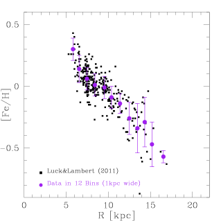
Figure 1: Radial abundance gradient for iron from observations of Cepheids. The data (black filled squares) are taken by Luck & Lambert (2011). The purple dots are the bins in which the data are divided, with their uncertainties. Each bin represents the mean abundance value in the stars located in proximity of each kpc, whereas the error bars are the standard deviation computed in each bin.

We also compare our model results with the data from HII regions and PNe. In this paper we adopt the HII region data by Deharveng et al. (2000), Esteban et al. (2005) and Rudolph et al. (2006), who analyzed the Galactic HII regions, and Costa et al. (2004) data for planetary nebulae (PNe). As for the Cepheids, the data for the sample PNe+HII regions have been treated in the same way, dividing them into twelve bins, each 1 kpc wide, as shown in Fig. 3.

We have computed the best fits to the abundance gradients for O and Fe from Cepheids on one hand, and from HII regions and PNe on the other hand. In particular, by using the least square method, the abundance gradients from the data of Cepheids of Luck & Lambert (2011) are:

$$\frac{d\left[\mbox{Fe/H}\right]}{dr}=-0.063\pm 0.003\ \mbox{dex/kpc\ \ (5-17\ kpc)},$$ (14)

$$\frac{d\left[\mbox{O/H}\right]}{dr}\,\,=-0.057\pm 0.003\ \mbox{dex/kpc\ \ (5-17\ kpc)}.$$ (15)

The data set for HII regions and PNe suggest for the oxygen the follow gradient:

$$\frac{d\left(log\left(\frac{O}{H}\right)+12\right)}{dr}=-0.059\pm 0.005\ \mbox{dex/kpc\ \ (2-18\ kpc)}.$$ (16)

It is worth noting that the Cepheid gradient obtained by Luck & Lambert (2011) is in excellent agreement with the gradient derived for HII regions and PNe.

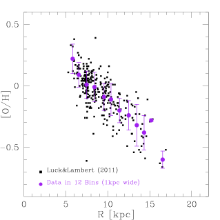
Figure 2: Radial abundance gradient for oxygen from observations of Cepheids. The data (black filled squares) are taken by Luck & Lambert (2011). The purple dots are the bins in which the data are divided, with their uncertainties. Each bin represents the mean abundance value in the stars located in proximity of each kpc, whereas the error bars are the standard deviation computed in each bin.

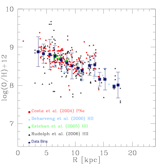
Figure 3: Radial abundance gradient for oxygen from observations. The data are taken by Deharveng et al. (2000) (light-blue crosses), Rudolph et al. (2006) (black triangles), Esteban et al. (2005) (green squares) for the HII regions and by Costa et al. (2004) (red filled circles) for the PNe.

In this work we also discuss the formation and the temporal evolution of the abundance gradients of different elements. To study their evolution in time, we need to compare our model results to the abundances as functions of the Galactocentric distance at various evolutionary stages. To compare our predictions we then need to find abundance data samples at redshift higher than zero. Unfortunately, abundance gradients at earlier times than the present one are very uncertain, such as for example those derived from old PNe. Some PNe could be in fact as old as 8-10 Gyr (PNe of type III) , whereas others are relatively young (PNe of type I). Maciel & Costa (2009) and Maciel & al. (2013) suggested a flattening of the gradient of O in the last 6-8 Gyr but the error on the estimated ages are probably too large to derive any firm conclusion. Recent data from Cresci et al. (2010) report oxygen abundances across three star-forming galaxies at redshift z $\sim$ 3. In this study, we consider two Lyman-Break galaxies, $SSA22a-C16$ at $z=3.065$ and $SSA22a-M38$ at $z=3.288$ which have similar properties to our Milky Way: each of them are star forming galaxies with masses, found assuming an exponential disk mass model to reproduce the dynamical properties of these sources, in the range $10^{10}-2\cdot 10^{12}\ M_{\odot}$, comparable with the mass of our Galaxy (see Table 1). In particular, in Table 1 we show the name of the galaxies, their redshifts, the estimated masses, the O abundances integrated over the whole galaxies as well as the O abundances in the low and high metallicity regions. The most striking result of this study is the existence of a large positive gradient in the oxygen abundance, in other words the O abundance in these galaxies seem to decrease towards the galactic centre. Although the data refer to regions in small galactocentric distance ranges (see Table 2) they clearly indicate a “gradient inversion” at redshift z=3. In particular, in Table 2 are reported the abundance gradients for the two Lyman Break galaxies obtained by considering the location (in kpc from the galactic centers) of the low and high metallicity regions, as defined in Cresci et al. (2010). In this paper we aim at understanding if this inversion is predicted by chemical evolution models and what can be its physical meaning.

Source	Redshift	Mass	$log(O/H)+12$
Name	$z$	$log\left(\frac{M_{\star}}{M_{\odot}}\right)$	(tot)	(low Z)	(high Z)
SS22a-C16	3.065	$10.68^{+0.16}_{-0.54}$	$8.36^{+0.06}_{-0.06}$	$8.18^{+0.13}_{-0.14}$	$8.52^{+0.14}_{-0.07}$
SS22a-M38	3.288	$10.86^{+0.18}_{-0.41}$	$8.26^{+0.09}_{-0.11}$	$7.84^{+0.22}_{-0.23}$	$8.59^{+0.05}_{-0.07}$

Table 1: Oxygen abundances by Cresci et al. (2010) at z=3. $z$ is the source redshift, $M_{\star}$ the stellar mass, while the last three columns show the metallicity integrated for the whole galaxy, for the low metallicity region and for the high metallicity regions respectively, in units of $12+log(O/H)$. The uncertainties are $1\ \sigma$ confidence interval.

Name	z	$log\left(\frac{M_{\star}}{M_{\odot}}\right)$	$\frac{d[log(O/H)+12]}{dRg}$ (range [kpc])
SS22a-C16	3.065	$10.68^{+0.16}_{-0.54}$	+0.13 (1.9-4.6)
SS22a-M38	3.288	$10.86^{+0.18}_{-0.41}$	+0.50 (1.9-3.4)

Table 2: Oxygen abundance gradients from two different metallicity zones in each galaxy at $z\sim 3$.

6 Model results

We use as a reference model an updated version of the Chiappini et al. (2001) model which corresponds also to the best model in Cescutti et al. (2007). First of all, we investigate in details the effects of several physical processes on abundance gradients:

• The inside-out formation of the thin disk, obtained by varying $\tau_{D}$ as a function of the galactocentric distance;

• The presence of a threshold in the gas density for star formation;

• A variable efficiency of star formation with the galactocentric distance;

• The radial gas flows and their velocity pattern

Table 3: The list of the models described in this work.

Model	Threshold [M⊙ pc-2]	$\tau_{d}$ (I-O) [Gyr]	$\sigma_{h}(r)$ [M⊙ pc-2]	SFE $\nu$ [Gyr-1]	Radial inflow
S-A	7 (Thin Disk)	1.033 R (kpc) -1.27 Gyr	17	1	/
	4 (Halo-Thick Disk)
S-B	7 (Thin Disk)	1.033 R (kpc) -1.27 Gyr	17	$\nu(R)\propto R^{-1}$	/
	4 (Halo-Thick Disk)			Colavitti et al. (2009)
S-C	/	1.033 R (kpc) -1.27 Gyr	17	1	/
S-E	7 (Thin Disk)	3 Gyr	17	1	/
	4 (Halo-Thick Disk)
S-G	/	1.033 R (kpc) -1.27 Gyr	17 if R$\leq 8$ kpc	1	/
			0.01 if R$\geq 10$
R-A	7 (Thin Disk)	1.033 R (kpc) -1.27 Gyr	17	1	velocity pattern I
	4 (Halo-Thick Disk)
R-B	7 (Thin Disk)	1.033 R (kpc) -1.27 Gyr	17	$\nu(R)\propto R^{-1}$	velocity pattern I
	4 (Halo-Thick Disk)			Colavitti et al. (2009)
R-C	7 (Thin Disk)	1.033 R (kpc) -1.27 Gyr	17	1	velocitiy pattern II
	4 (Halo-Thick Disk)
R-D	/	1.033 R (kpc) -1.27 Gyr	17 if R$\leq 8$ kpc	1	velocitiy pattern III
			0.01 if R$\geq 10$

In Table 3 all the models considered in this work are reported. The model names are shown in the first column: the letter “S” means that it is a static model, namely without any radial inflow in the disk, while “R” stands for the models that take into account the radial flows. If a threshold is present in the model, its values for the halo and thin disk phases are shown in the second column, expressed in $M_{\odot}pc^{-2}$. The inside-out scenario is expressed by a linear variation of the timescale of infall $\tau_{D}(R)$, as shown in eq. (6), and if this assumption is absent, the timescale is set to be constant having a value of 3 Gyr. In column 4 is indicated the assumed total (stars plus gas) surface mass density profile of the halo in $M_{\odot}pc^{-2}$ (see Chiappini et al. 2001). In column 5 the SFR is indicated. The variable SFE $\nu(R)$ assumes different values at different galactocentric distances, as in the work by Colavitti et al. (2009). This approach is not new since a variable $\nu$ has already been proposed on the basis of large-scale instabilities in rotating disks (e.g. Boissier & Prantzos 1999; Boissier et al. 2001). We assume a star formation efficiency (SFE) that increases towards the innermost regions of the disk. For $R\leq 14$ kpc the efficiency is $\nu\propto R^{-1}$, while in the outer parts of the disk we assume a constant value of $\nu=0.03$ Gyr^-1; the reason is that in these outer regions the gas density is very small and decreasing exponentially, so assuming a decreasing $\nu$ would lead to a very small value for this parameter and consequently to negligible star formation.

Lacey and Fall (1985) studied the Galactic chemical evolution in the presence of radial inflow of gas and demonstrated that such flow enhances the metallicity gradient within the disk. As shown in Schönrich and Binney (2009) and Spitoni & Matteucci (2011), to reproduce the data it is necessary to adopt a variable velocity for the radial gas flow. In this situation, each ring has its own velocity inflow. Here we use several velocity patterns, shown in Fig. 4. The velocities in these patterns always decrease inwards (in agreement with Edmunds & Greenhow 1995), and in modulus they span the range 0-5 km sec^-1 , in accordance with the results of Schönrich and Binney (2009) and other previous works in literature (Wong et al. 2004; Lacey & Fall 1985; and Tinsley 1980).

Our radial inflow patterns are in accordance with the ones computed by Bilitewski & Schönrich (2012), imposing the conservation of the angular momentum. Fu et al. (2013) in semi-analytic models of disk galaxy formation have taken into account a radial inflow of gas in agreement with this work and Spitoni & Matteucci (2011). Moreover, Wang & Zhao (2013) presented a chemical evolution model for the Milky Way including stellar migration and radial inflows of gas, and again the chosen patterns are in agreement with our models.

6.1 The present day gradient results

In Figs. 5 and 6 we show our results for the oxygen and iron present day gradient, respectively, compared with the data from Cepheids. The model labeled S-A is our reference model and it is just an updated version of the Chiappini & al. (2001) Model B. The Galactic disk in this model forms inside-out; this means that the inner parts are assembled before the outer ones. This kind of formation is quite successful in reproducing the main features of the Milky Way as well as of the external galaxies, especially concerning abundance gradients (e.g. Matteucci & François, 1989; Chiappini et al. 2001; Prantzos & Boissier 2000; Pilkington et al. 2012).

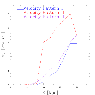
Figure 4: Radial inflow velocity profiles adopted in this paper (see text).

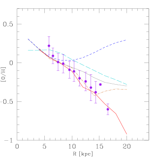
Figure 5: Effect on the oxygen abundance gradients of the four parameters that characterize the chemical evolution models where the halo surface density is fixed at the value of $\sigma_{H}=17$ M_⊙ pc^-2: threshold (model S-C, blue short dashed line), Inside-Out (model S-E, light-blue long dashed line), variable SFE (model S-B, brown dashed line) and radial flows (model R-A, red solid line). The black dotted line represents the static model by Chiappini et al. (1997), model S-A with Inside-Out, threshold, constant SFE and without inflow. The data are by Luck & Lambert (2011).

If instead we do not assume an inside-out formation for the thin disk, and keep constant the timescale of infall $\tau_{D}$ , the present day abundance gradients provided by the model are too flat in the inner part of the disk, as shown by the model S-E in both Figs. 5 and 6, even if a threshold in the gas density is assumed. In fact, the threshold influences mostly the outer gradient.

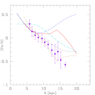
Figure 6: Effect on the iron gradients of the four parameters that characterize the chemical evolution models where the halo surface density is fixed at the value of $\sigma_{h}=17$ M_⊙ pc^-2: threshold (model S-C, blue short dashed line), Inside-Out (model S-E, light-blue long dashed line), variable SFE (model S-B, brown dashed line) and radial flows (model R-A, red solid line). The black dotted line represents the static model by Chiappini et al. (1997), model S-A with Inside-Out, threshold, constant SFE and without inflow. The data are by Luck & Lambert (2011).

From Figs. 5 and 6 it is clear that without a threshold in the standard static model (model S-C), even if an inside-out formation is considered, the gradient is too flat between 6-12 kpc and in the outer parts of the disk it even increases, clearly at variance with the observational data. The reason why the threshold steepens the gradient in the outermost regions is because every time the gas density goes below the critical value (and it is easier to happen in the outer regions), the star formation stops and starts again only when the gas has gone over the threshold thanks to gas infalling and/or restored by dying stars. Actually, at distances larger than 15-16 kpc the gas density is almost always below the assumed threshold so the abundances are very low, due to the frequent suppression of star formation. This is in agreement with what found in Chiappini et al. (2001). Thus, we can conclude that a threshold in the gas density seems to be necessary to have the right trend of the gradients in the outer parts of the disk in a static model with the inside-out formation. The model which assumes a variable SFE, a threshold, and inside-out formation (model S-B), provides a good fit to the observed present day abundance gradients from 4 to 14 kpc. However, beyond this distance the gradient predicted by the models is too flat and inconsistent with the observations. This is due to the fact that we have assumed a constant and very low ($\nu=0.03$ Gyr^-1) SFE at distances $>14$ kpc. Finally, the model R-A assumes the presence of a radial gas inflow following the velocity pattern (pattern I) similar to that adopted in Spitoni & Matteucci (2011) and shown in Fig. 4. Using this velocity pattern for the radial inflow, we can see from Fig. 5 that the oxygen gradient provided by the model R-A (-0.058 $\pm$ 0.005) is steeper than the one predicted by the static model S-A (-0.030 $\pm$ 0.002), and in better agreement with the observational data. In Fig. 7 we show that the model R-A perfectly fits also the gradient observed in the HII regions and PNe.

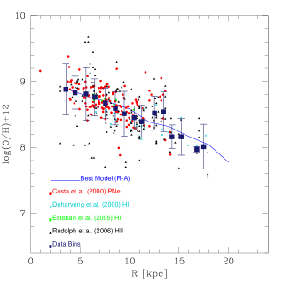
Figure 7: Comparison between the data set composed by HII regions and PNe for the oxygen, and the R-A model predictions. This model assumes Inside-Out formation, a threshold in the gas density, and radial inflow of gas with the velocity pattern taken by Spitoni & Matteucci (2011)

However, it is clear from Fig. 6 that the Fe gradient from model R-A does not fit the present time gradient, at least in the outer regions, and in any case the fit is worse than in the static model S-A. In particular, in the presence of radial flows with the velocity pattern I the Fe gradient flattens between 9 and 14 kpc. So, with this kind of radial flows the O gradients steepens, whereas that of Fe flattens.

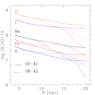
Figure 8: Present day abundance gradients for O, C, Ne, Fe, and S for the static model S-A (solid lines) and for the model with radial inflow of gas R-A (dashed lines).

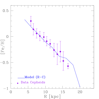
Figure 9: Iron abundance gradient: comparison between observations and model (R-C) predictions. This fit is obtained using the velocity pattern (II) shown in Fig. 4. The data are taken from Luck & Lambert (2011).

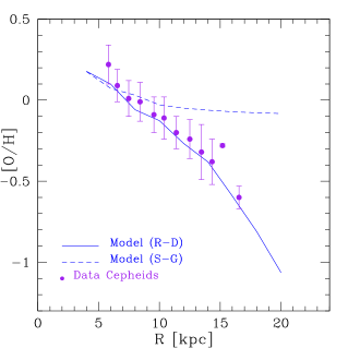
Figure 10: Oxygen abundance gradient: comparison between observations and model (S-G) and (R-D) predictions. The best fit in the model (R-D) is obtained using the velocity pattern (III) shown in Fig. 4. The data are taken from Luck & Lambert (2011).

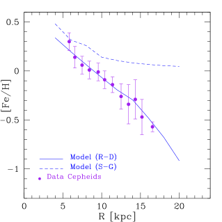
Figure 11: Iron abundance gradient: comparison between observations and model (S-G) and (R-D) predictions. The best fit in the model (R-D) is obtained using the velocity pattern (III) shown in Fig. 4. The data are taken from Luck & Lambert (2011).

In the past, several authors have suggested that the main effect of taking into account radial gas flows in chemical evolution models is the steepening of the abundance gradients. It is interesting to note that in the majority of previous works, only the O gradient was discussed in relation to radial flows. However, in Spitoni & Matteucci (2011) it was shown that for a model with just one infall, aimed at studying just the disk and not the whole Galaxy as the two-infall model, a linear law for the gas flow velocity could reproduce both the O and Fe gradient at the same time. On the other hand, also in Bilitewski & Schönrich (2012), who included radial gas flows in their model, a flat gradient in the central disk region was found for the iron in some of their models. The explanation of this behavior can be found in the combination of several processes:

• different timescales of production of chemical elements (oxygen is produced on short time scales whereas iron on long ones);

• the two-infall assumption for the gas accretion, in particular the assumed total surface mass density distribution for the halo;

• the inflow velocity pattern considered.

In particular, it seems that the flattening of the Fe gradient in the central disk regions could be due to a combination of variable velocity for the flow and long timescales for the Fe production from Type Ia supernovae. To test our hypothesis, we computed the gradients of other elements, as shown in Fig. 8, where we report the predictions for the gradients of O, Fe, C, Ne, and S, obtained with model R-A. As expected, the elements produced on short time scales, such as O and Ne show a steeper gradient relative to the static case, whereas the ones produced on long time-scales, such as C, show the same behavior as Fe. This means that with that particular velocity pattern for radial flows (pattern I), the elements produced on long timescales flatten in the central part of the disk.

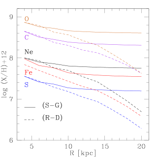
Figure 12: Present day abundance gradients for O, C, Ne, Fe, and S for the static model S-G (solid lines) and for the model with radial inflow of gas R-D (dashed lines).

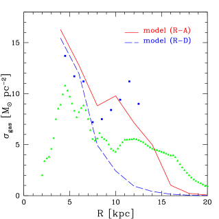
Figure 13: The surface gas density profile as a function of the radial distance for the model (R-D) drawn with the blue dashed line and for the model (R-A) drawn with solid red line. The green triangles represent the data of Dame et al. (1993), whereas the blue squares the data of Rana (1991).

Having said that, the problem remains that model R-A does not fit the present day Fe gradient. This is clearly a peculiarity of the two-infall model since Spitoni & Matteucci (2011) could fit both Fe and O gradients at the same time with a simple linear velocity pattern in the framework of the one-infall model. We have then tried another velocity pattern that can fit the Fe gradient and we have found that, in order to obtain a good fit to the present day Fe gradient we need to assume for Fe a different velocity pattern, as shown in Fig. 4 (velocity pattern II). In particular, we need a strong decrease in the inflow velocity towards the Galactic centre. With this velocity pattern, the iron abundance gradient can be very well reproduced, as shown in Fig. 9. The value of this gradient is:

$$\frac{d\left[\mbox{Fe/H}\right]}{dr}=-0.064\pm 0.004\ \mbox{dex/kpc\ \ (5-17\ kpc)}.$$ (17)

However, the gradient of O in this case is no more in good agreement with the data.

We have then finally tested a model with a total surface mass density in the halo becoming very small for distances $>$ 10 kpc (model R-D), a more realistic situation than that in model R-A, and yet a different velocity pattern (III). In this case we were able to find a very good agreement for both O and Fe present day gradient, as shown in Figs. 10 and 11. In these figures are shown also the predictions by the equivalent static model S-G. It is clear that this latter cannot reproduce the present time gradients because it does not assume any threshold in the gas density nor radial flows. In Fig. 12 we report the present day abundance gradients for O, C, Ne, Fe, and S for the model R-D with radial flow and for the equivalent static model S-G. In contrast to model R-A (Fig. 8), we see that in the model R-D all elements show a steeper gradient compared to the relative static model S-G, without any flattening in the central parts for elements produced on long time-scales. The peculiarity of models R-D and S-G is that the halo surface mass density is assumed to drop dramatically for galactocentric distances larger than 10 kpc. Therefore, the halo surface mass density distribution seems to play an important role in shaping the gradients especially in the presence of radial gas flows. The halo surface mass density can influence, in fact, the gas distribution in the disk at large galactocentric distances, as already discussed in Chiappini et al. (2001). Assuming a constant surface density of 17 M_⊙ pc^-2 for the halo is also not realistic for distances larger than 10 kpc where the surface mass density of the disk is much smaller. So, our best model is model R-D.

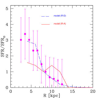
Figure 14: The SFR normalized to the solar values as a function of the galactocentric distance for the (R-A) and (R-D) models. The data are taken by Rana (1991) and are reported with the magenta points and relative error bars.

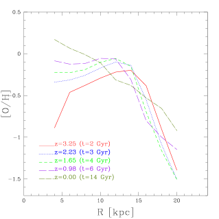
Figure 15: Evolution with redshift of the abundance gradients for the model R-A for the Oxygen. Model R-A assumes a threshold, Inside-Out formation, constant SFE and radial flows. The evolution is studied by computing the abundance gradients for the redshifts z=3.25, 2.23, 1.65, 0.98 and 0.0 whose correspond to the times t=2, 3, 4, 6 and 14 Gyr after the Big Bang (in a $\Lambda CDM$ cosmology).

We pass now to analyze how the profile of the gas along the Galactic disk is modified with the velocity patterns used for the best model (R-D) and the model (R-A). In Fig. 13, we compare our results for the gas surface density profile as a function of the radial distance with the data of Dame et al. (1993) and Rana (1991). As stated in Spitoni & Matteucci (2011), the main effect of the radial inflow with a variable velocity is to concentrate the gas in the inner regions of the Galaxy. In the inner regions between 5 and 8 kpc our results are in very good agreement with the data of Rana (1991). On the other hand, both the models (R-D) and (R-A) underestimate the gas density in the outer regions, but the model (R-A) shows agreement with the data of Rana (1991) between 8 and 14 kpc. Our models, like the majority of the others, are not able to reproduce the decrease in gas density for R $\leq$ 5 kpc of Dame et al. (1993). This is probably because the effect of bar is not considered.

In Fig. 14 the SFR along the disk of the Galaxy for the (R-D) and (R-A) models is compared with the data of Rana (1991). In this figure we show the SFR normalized to the solar value as a function of the Galactocentric distance. Because of the uncertainties in this data set, as it can be seen from the large error bars, we cannot draw firm conclusions, although the model (R-D) seems to fit the data very well. On the other hand, model (R-A) underestimates the $SFR/SFR_{\odot}$ for R $\leq$ 6 kpc, but its results are consistent with observations within the error bars given by one standard deviation.

6.2 The high redshift gradients

We show in Figs. 15 and 16 the temporal evolution of the gradients for the model (R-A) and the model with variable SFE (R-B) for the oxygen. Concerning the R-A model (that assumes a constant SFE) at z=3, corresponding to a cosmic time of 2 Gyr in a $\Lambda$CDM cosmology, the gradient reveals the inversion of the gradient, i.e. a positive value in the inner regions of the disk. Then the gradient exhibits a steepening in time, mostly in the inner regions, and at z=0.98 the gradient inversion disappears, giving way to a plateau in the inner parts of the disk. After that, the steepening continues until the gradient reaches the known shape at the present time. If we look at the temporal evolution for the model R-B, it is evident that by assuming a variable SFE, the gradient inversion is never predicted. However, as in the case of the R-A model, the steepening with time is still present, and this is due to the threshold in the gas density.

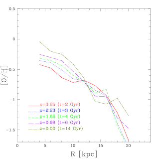
Figure 16: Evolution with redshift of the abundance gradients for the model R-B for the Oxygen. Model R-B is the same of the one R-A but with variable SFE. The evolution is studied by computing the abundance gradients for the redshifts z=3.25, 2.23, 1.65, 0.98 and 0.0 whose correspond to the times t=2, 3, 4, 6 and 14 Gyr after the Big Bang (in a $\Lambda CDM$ cosmology).

Finally, we present in Fig. 17 the temporal evolution for our best model R-D. We recall that this model is able to fit the present day abundance gradients both for O and Fe by means of the same pattern of gas flow velocity (pattern III in Figure 4). Moreover, at z=3 the model presents the inversion of the gradient, but less pronounced than the model R-A. As expected, the abundance gradient steepens in time. Using the same models listed in Table 3, we derived the abundance gradients at the time t = 2 Gyr. The results are shown in Table 4 where are reported the theoretical abundance gradients predicted by our models and their uncertainties. They were computed by means of the least square method, as done for the present day gradients. In the fitting procedure, we considered only the inner range of the thin disk (2-8 kpc) for a better comparison with the data by Cresci et al. (2010).

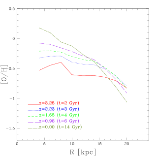
Figure 17: Evolution with redshift of the abundance gradients for the best model R-D for the oxygen. The evolution is studied by computing the abundance gradients for the redshifts z=3.25, 2.23, 1.65, 0.98 and 0.0 whose correspond to the times t=2, 3, 4, 6 and 14 Gyr after the Big Bang (in a $\Lambda CDM$ cosmology).

Table 4: Abundance gradients at high redshift ($z=3$) predicted by models S-A, S-B, S-C, S-E, S-G, R-A, R-B, R-C, and R-D. The gradients were computed with the least square method and only in the inner parts of the thin disk, where the trend is approximated by a linear regression.

Model	Range	$\frac{d\left(log(O/H)+12\right)}{dRg}$	$\frac{d\left(log(Fe/H)+12\right)}{dRg}$
	[kpc]	[dex kpc-1]	[dex kpc-1]
SA	2-8	$+0.036\pm 0.009$	$+0.047\pm 0.008$
SB	4-8	$-0.066\pm 0.008$	$-0.066\pm 0.003$
SC	2-8	$+0.038\pm 0.007$	$+0.045\pm 0.009$
SE	4-8	$+0.022\pm 0.004$	$+0.034\pm 0.001$
SG	4-8	$+0.039\pm 0.004$	$+0.060\pm 0.001$
RA	4-8	$+0.128\pm 0.050$	$+0.060\pm 0.002$
RB	4-8	$-0.054\pm 0.014$	$-0.053\pm 0.014$
RC	4-8	$+0.035\pm 0.002$	$+0.049\pm 0.003$
RD	4-8	$+0.034\pm 0.049$	$+0.050\pm 0.005$

As it is evident from Table 4, if we look at the abundance gradients at high redshift, both iron and oxygen exhibit a gradient inversion in the inner part of the disk. In other words, if we consider for example the gradients of our best model (R-D, red solid lines), at t = 2 Gyr, they show an increase of metallicity from the outer regions up to 10 kpc where they reach a peak and then a decrease for R $<$ 10 kpc. This is not true for the model (S-B) with variable SFE: this model predicts a negative abundance gradient even at high redshift. This theoretical gradient inversion in the innermost part of the disk is confirmed by the data taken by Cresci et al. (2010) (only for the oxygen because only for this element there are available metallicity measurements), which found positive gradients for both of the galaxies considered (see Table 2). Our high redshift positive gradients are in general smaller than the observed ones: the reason for this could reside in the nature of the sources used to derive the metallicity at high redshift. In fact, in the sample by Cresci et al. (2010), there are Lyman-Break galaxies showing evidence for disk. However these galaxies might be large objects than the Milky Way and this could be the reason for our gradients being smaller.

Our explanation for the gradient inversion in the Milky Way is based on the inside-out disk formation:

• at early epoch (t=2 Gyr from the Big Bang, z = 3) the efficiency of chemical enrichment (i.e. of the SFR), in the inner regions is high but the rate of infalling primordial gas is dominating, thus diluting the gas more in the inner regions than in the outer ones;

• as time passes by, the infall of pristine gas in the inner parts decreases and the chemical enrichment takes over;

• then, at later epochs, the SFR in the inner regions is still much higher than in the outer parts of the disk where the gas density is very low, but the infall is lower and the abundance gradients assume the shape seen in the observational data.

Since we assumed a flow velocity constant in time we checked the robustness of our results for the (R-D) model concerning the inversion of gradient at redshift z=3, considering a time-dependent velocity pattern consistent with the present time pattern III introduced in Fig. 4, and with the work of Bilitewski & Schönrich (2012).

We assume for this test the extreme case where the pattern III is the present day law, and we look for the pattern at times $t\leq 2$ Gyr which could end up as pattern III. In Fig. 3 of Bilitewski & Schönrich (2012), time dependent velocity patterns at times $t=$ 3 Gyr, 6 Gyr, 9 Gyr, and 12 Gyr are presented. We find that the radial velocity pattern at 3 Gyr is related to the one at 12 Gyr by the following expression: $v_{r}(3\ Gyr)=1.37\times v_{r}(12\ Gyr)$.

Therefore, for the model (R-D) we assume that the pattern at the early times up to 2 Gyr follows this equation:

$$v_{r}(t\leq 2\ Gyr)=1.5\times v_{r}(patternIII).$$ (18)

In Fig. 18, we labeled this velocity profile as “pattern V”. In Fig. 19 we show the abundance gradient for the oxygen at t=2 Gyr using this new velocity pattern, and we can see that the inversion of the gradient is preserved. We consider this a robust test.

On the other hand, a full treatment of a time dependent velocity pattern is not the aim of this paper and it will be discussed in a future work.

The last test was to check a smaller velocity of the flow at 2 Gyr (pattern IV in Fig. 18). In Fig. 19 we can see that also in this case a gradient inversion is present.

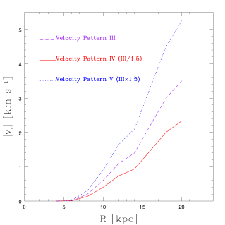
Figure 18: Radial inflow velocity used to check the inversion of gradient at high redshift: velocity pattern III (dashed magenta line), IV (red solid line), V (blue dotted line). We applied these patterns to the model (R-D) up 2 Gyr.

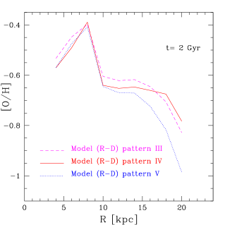
Figure 19: (R-D) model predictions for Oxygen abundance gradient at 2 Gyr using the velocity pattern III (dashed magenta line), IV (red solid line), V (blue dotted line) shown in Fig. 18.

7 Conclusions

We have computed the chemical evolution of the Milky Way with particular attention to the formation and evolution of the abundance gradients. We have tested the effects of several physical processes which can influence the formation of gradients, and studied the temporal evolution of gradients. In particular, we have tested whether the gradient inversion of redshift z=3 is preserved in the presence of radial gas flows, and this is the main novelty of the paper.

Our main conclusions can be summarized as follows:

• If we do not assume an inside-out formation for the thin disk ($\tau_{D}$ constant), the present day abundance gradients provided by the model are too flat in the inner part of the disk and the observations are not reproduced (model S-E).

• Without a threshold in the standard static model by Chiappini et al.(2001) even if an inside-out formation is considered (model S-C), the gradient is too flat between 6-12 kpc and, mostly in the outer parts of the disk, the observational data are not reproduced. The threshold steepens the gradient in the outermost regions.

• To reproduce the abundance gradients in the whole disk, it is not possible to assume a variable SFE (model S-B) because, with this assumption, a flat gradient in the outer part of the thin disk is necessarily obtained (R $>$ 14 kpc). The use of a constant $\nu$ = 1 Gyr⁻¹ along the whole disk is the best choice to reproduce the chemical evolution of the Milky Way.

• The best model we found (R-D) assumes inside-out formation of the disk, a constant efficiency of SF along the disk, a surface halo mass density decreasing with galactocentric distance and radial gas flows with a velocity pattern predicting a decrease of the speed of the gas flow for decreasing galactocentric distance in the range between 0 and 3.8 km s^-1.

• We found that the assumed velocity pattern for radial gas flows is a crucial parameter in shaping the chemical evolution of the disk and in particular the abundance gradients and their evolution.

• All the chemical evolution models presented here show a steepening of the gradient in time, mostly in the inner regions.

• At z=3 a gradient inversion in the inner regions of the thin disk is predicted for most of our chemical evolution models, including the best one. With a time dependent velocity radial inflow, the inversion of the abundance gradient at early times is preserved.

  This inversion is observationally confirmed (Cresci et al. 2010) and is interpreted as due to the strong infall of primordial material at early times in the innermost disk regions, as predicted by the inside-out formation. Therefore, the gradient inversion is a direct consequence of the inside-out disk formation.

• The only model with inside-out that does not predict the gradient inversion at high redshift is that with variable SFE (model S-B). In this model the gradient at z = 3 is negative as the present day one. If the gradient inversion will be confirmed, we can conclude that a variable the SFE, which contrasts the effect of the infall at early times, is unlikely.

• Finally, a word of caution is necessary relative to the observed gradient inversion at high z; Yuan et al. (2003) showed that the measured metallicity gradient changes systematically with angular resolution and annular binning. Seeing-limited observations produce significantly flatter gradients than higher angular resolution observations. For these reasons, more observations are needed in the future to confirm Cresci et al. (2010) high redshift positive inner gradients.

It is worth, before concluding, to discuss how robust are the above conclusions. We run several models changing the main assumptions which are: inside-out formation of the disk, efficiency of star formation, radial flows and their speed, threshold gas density for star formation and distribution of the total surface mass density of the Galactic halo. The inside-out formation scenario is a well tested assumption suggested by the majority of papers concerning the Galactic disk (e.g. Pilkington et al. 2012) and also by observations at high redshift (e. g. Mateo-Munoz et al. 2007). We conclude that the inside-out formation is necessary to reproduce the abundance gradients but also to obtain a gradient inversion at high redshift and this is a robust conclusion. In fact, even changing all the other physical processes, with the exception of a variable star formation efficiency with galactocentric distance, a model with inside-out always predict such an inversion.

On the other hand, other assumptions are probably still debatable, such as the halo total surface mass density distribution. This might appear like a quantity which should not influence abundance gradients in the disk. Instead, this quantity has a noticeable influence on the disk gradients at large galactocentric distances. In fact, at such distances the total surface mass density of the disk is negligible and that of the halo might predominates. This fact was already discussed in Chiappini et al. (2001). We find that both the O and Fe gradient at the present time in the disk can be well reproduced if the halo total surface mass density distribution is a strong decreasing function of the galactocentric radius, but we cannot say if this is an unique solution.

A variable efficiency of star formation with radius can be certainly ruled out if the gradient inversion will be confirmed and this is also a robust result.

On the other hand, the presence or absence of a gas density threshold cannot be firmly established on the basis of our models, although in the presence of radial flows we obtain better results without a threshold.

Finally, the model could be further improved by considering stellar migration in the disk which will be the subject of a forthcoming paper.

References

- Andrievsky et al. (2002) Andrievsky, S.M., Bersier, D., Kovtyukh, V. V. et al 2002a, A&A, 384, 140
- Andrievsky et al. (2002) Andrievsky, S.M., Kovtyukh, V.V., Luck R.E. et al 2002b, A&A, 381, 32
- Andrievsky et al. (2002) Andrievsky, S. M., Kovtyukh, V. V., Luck, R. E., et al. 2002c, A&A, 392, 491
- Andrievsky et al. (2004) Andrievsky, S. M., Luck, R. E., Martin, P., et al. 2004, A&A, 413, 159
- Asplund et al. (2009) Asplund, M., Grevesse, N., Sauval, A. J., Scott, P., 2009, ARA&A, 47, 481
- Asplund et al. (2005) Asplund, M., Grevesse, N., & Sauval, A. J. 2005, in Cosmic Abundances as Records of Stellar Evolution and Nucleosynthesis, ed. T. G. Barnes III, F. N., Bash, ASP Conf. Ser., 336, 25
- Cescutti et al. (1996) Bertin G., Lin C.C., 1996, Spiral structure in galaxies – A density wave theory, MIT Press, Cambridge, Massachusetts
- bilitewski et al. (2012) Bilitewski, T., & Schönrich, R. 2012, MNRAS, 426, 2266
- boisser et al. (1999) Boisser, S., Prantzos, N., 1999, MNRAS, 307, 857
- boisser et al. (2000) Boisser, S., Prantzos, N., 2000, MNRAS, 312,398
- cescutti et al. (2006) Cescutti, G., Francois, P., Matteucci, F., Cayrel, R., Spite, M., 2006, A&A, 448, 557
- Cescutti et al. (2007) Cescutti, G., Matteucci, F., Francois, P., & Chiappini, C. 2007, A&A, 462, 943
- Chiappin et al. (1997) Chiappini C., Matteucci F., & Gratton R., 1997, ApJ, 477, 765
- Chiappini et al. (2003) Chiappini C., Matteucci F., & Meynet G., 2003, ApJ, 410, 257
- Chiappini et al. (2001) Chiappini C., Matteucci F., & Romano D., 2001, ApJ, 554, 1044
- chiosi (1980) Chiosi C., 1980, A&A 83, 206
- Colavitti et al. (2009) Colavitti. E., Cescutti, G., Matteucci F., Murante G., 2009, A&A, 496, 429
- Contini et al. (2011) Contini, T., Epinat, B., Queyrel, J., Vergani, D., Tasca, L., Amram, P., Garilli, B., 2011, arXiv:1103.5579
- Costa et al. (2004) Costa, R. D. D., Uchida, M. M. M., & Maciel, W. J. 2004, A&A, 423, 199
- cresci (2010) Cresci, G., Mannucci, F., Maiolino, R., Marconi, A., Gnerucci, A., Magrini, L., 2010, Nature, 467, 811
- Curir (2012) Curir, A., Lattanzi, M. G., Spagna, A., Matteucci, F., Murante, G., Re Fiorentin, P., Spitoni, E., A&A, 545, A133
- Dame (1993) Dame, T. M., 1993, in Back to the Galaxy, ed. S. Holt & F. Verter (New York: AIP), 267
- Deharveng et al. (2000) Deharveng, L., Peña, M., Caplan, J., & Costero, 2000, MNRAS, 311, 329
- esteban et al. (2005) Esteban, C., García-Rojas, J., Peimbert, M., Peimbert, A., Ruiz, M. T., Rodriguez, M., Carigi, L., 2005, ApJ, 618, 95
- François et al. (2004) François P., Matteucci F., Cayrel R., Spite, M., Spite, F., & Chiappini, C., 2004, A&A, 421, 613
- Fu (2013) Fu, J., Kauffmann, G., Huang, M., Yates, R. M., Moran, S. H., Timothy M., Dave, R., Guo, Q., Henriques, B. M. B., 2013, arXiv1303.5586
- Götz & Köppen (1992) Götz, M., Köppen, J., 1992, A&A, 262, 455
- Greggio & Renzini (1983) Greggio L.,& Renzini A., 1983, A&A, 118, 217
- Kennicutt (1989) Kennicutt, R. C., Jr., 1989, ApJ, 344, 685
- Kennicutt (1998) Kennicutt, R. C., Jr., 1998, ApJ, 498, 541
- iwamoto (1999) Iwamoto, K., Brachwitz, F., Nomoto, K., et al. 1999, ApJ Suppl. Ser. 125, 439
- jones (2010) Jones, T., Ellis, R., Jullo, E., Richard, J., 2010, ApJ, 725, L176
- lacey (1985) Lacey C.G., Fall M., 1985, ApJ, 290, 154
- luck (2003) Luck, R. E., Gieren, W. P., Andrievsky, S. M., et al. 2003, A&A, 401, 939
- luck (2011) Luck, R. E., Lambert, D. L., 2011, AJ, 142, 136
- luck (2011) Luck, R. E., Andrievsky, S. M., Kovtyukh, V. V., Gieren, W., Graczyk, D., 2011, AJ, 142, 51
- Maciel (2009) Maciel, W. J., Costa, R. D. D., 2009, IAUS, 254, 38
- Maciel (2013) Maciel, W. J., Rodrigues, T., Costa, R. D. D., 2013, in “Planetary Nebulae: An Eye to the Future”, Proceedings of the International Astronomical Union, IAU Symposium, Volume 283, p. 424
- Maeder (1989) Maeder, A., & Meynet, G., 1989, A&A, 210, 155
- Mannucci et al. (2005) Mannucci, F ., Della Valle, M., Panagia, N., Cappellaro, E., Cresci, G., Maiolino, R., Petrosian, A., & Turatto, M, 2005, A&A, 433, 807
- uchida (2010) Marcon-Uchida, M.M., Matteucci, F., Costa, R.D.D., 2010, A&A, 520A, 35
- Martin (2001) Martin, C. L., & Kennicutt, R. C., Jr., 2001, ApJ, 555, 301
- Matteucci (2001) Matteucci, F., 2001, The Chemical Evolution Of The Galaxy, Kluwer Academic Publishers.
- Matteucci & François (1989) Matteucci, F., & François, P., 1989, MNRAS, 239, 885
- Matteucci & Greggio (1986) Matteucci M.F., Greggio L., 1986, A&A, 154, 279
- mayor (1981) Mayor M., Vigroux L., 1981, A&A 98, 1
- molla (2005) Molla, M., Diaz, A. I., 2005, MNRAS, 358, 521
- munoz (2007) Munoz-Mateos, J. C., Gil de Paz, A., Boissier, S., Zamorano, J., Jarrett, T., Gallego, J., Madore, B. F., 2007, ApJ, 658, 1006
- Pagel (1995) Pagel, B.E.J.,& Tautvaisiene, G., 1995, MNRAS, 276, 505
- Pilk (2012) Pilkington, K., Few, C. G., Gibson, B. K., et al. 2012, A&A, 540, A56
- Portinari chiosi (2000) Portinari, L., Chiosi, C., 2000, A&A, 355, 929
- Prantzos (2000) Prantzos, N., Boissier, S., 2000, MNRAS, 313, 338
- rana (1991) Rana, N. C. 1991, ARA&A, 29, 129
- reid (1993) Reid, M. J., 1993, ARA&A, 31, 345
- Rudolph et al. (2006) Rudolph, A. L., Fich, M., Bell, G.R., Norsen, T., Simpson, J.P., Haas, M.R., & Erickson, E.F., 2006, ApJS, 162, 346
- Scalo (1986) Scalo, J. M., 1986, FCPh, 11, 1
- schaye (2004) Schaye, J., 2004, ApJ, 609, 667
- binney (2009) Schmidt, M., 1959, ApJ, 129, 243
- scoen (2009) Schönrich, R., & Binney, J. 2009, MNRAS, 396, 203
- Sommer (1990) Sommer-Larsen J., Yoshii Y., 1990, MNRAS, 243, 468
- Spagna (2010) Spagna, A., Lattanzi, M. G., Re Fiorentin, P., Smart, R. L. 2010, A&A, 510, L4
- Spitoni (2011) Spitoni, E., & Matteucci, F. 2011, A&A, 531, A72
- Spitoni (2011) Spitoni, E., Matteucci, F., Marcon-Uchida, M. M., 2013, A&A, 551, A123
- Talbot (1973) Talbot, R., J., Jr., Arnett, W., D., 1973, 186, 51
- thon (1998) Thon R., Meusinger H., 1998, A&A, 338, 413
- Timmes et al. (1974) Timmes, F.X., Woosley, S.E., Weaver, T.A., 1995, ApJS, 98, 617
- Tinsley (1980) Tinsley, B. M. 1980, Fund. Cosmic Phys., 5, 287
- van den Hoek & Groenewegen (1997) van den Hoek L.B., & Groenewegen M.A.T. 1997, A&A Suppl., 123, 305
- wang (2013) Wang, Y., Zhao, G., 2013, arXiv:1303.7436
- wong (2004) Wong, T., Blitz, L., Bosma, A., 2004, Apj, 605, 183
- Woosley & Weaver. (1995) Woosley S.E., & Weaver, T.A., 1995, ApJ, 101, 181
- Yuan (2011) Yuan, T.,T., Kewley, L. J., A. M. Swinbank, A. M., Richard, J., Livermore, R. C., 2011, ApJ, 732, L14
- Yuan (2011) Yuan, T.,T., Kewley, L. J., Rich, L., 2013, ApJ, 767, 106