Anomalous non-additive dispersion interactions in systems of three one-dimensional wires

Abstract

The non-additive dispersion contribution to the binding energy of three one-dimensional (1D) wires is investigated using wires modelled by (i) chains of hydrogen atoms and (ii) homogeneous electron gases. We demonstrate that the non-additive dispersion contribution to the binding energy is significantly enhanced compared with that expected from Axilrod-Teller-Muto-type triple-dipole summations and follows a different power-law decay with separation. The triwire non-additive dispersion for 1D electron gases scales according to the power law $d^{-\beta}$, where $d$ is the wire separation, with exponents $\beta(r_{s})$ smaller than 3 and slightly increasing with $r_{s}$ from 2.4 at $r_{s}=1$ to 2.9 at $r_{s}=10$, where $r_{s}$ is the density parameter of the 1D electron gas. This is in good agreement with the exponent $\beta=3$ suggested by the leading-order charge-flow contribution to the triwire non-additivity, and is a significantly slower decay than the $\sim d^{-7}$ behaviour that would be expected from triple-dipole summations.

I Introduction

Recently there has been a resurgence in attempts to model the dispersion interaction between low-dimensional nano-scale objects more accurately. Using an array of electronic structure Spencer (2009); Misquitta et al. (2010); Drummond and Needs (2007) and analytical Dobson et al. (2006) techniques, several groups have demonstrated that the dispersion interaction between one- and two-dimensional systems can deviate strongly from that expected from the well-known additive picture of $r^{-6}$-type interactions Stone (2013); Kaplan (2005). For the case of parallel one-dimensional (1D) metallic wires separated by distance $d$, Dobson et al. Dobson et al. (2006) demonstrated that the van der Waals dispersion interaction should decay as $\sim-d^{-2}[\ln(\gamma d)]^{-3/2}$, where $\gamma$ is a constant that depends on the wire width. This analytic result was subsequently verified by Drummond and Needs Drummond and Needs (2007) using diffusion quantum Monte Carlo (DMC) calculations Foulkes et al. (2001). This change in the power-law of the dispersion energy can be understood as arising from correlations in extended plasmon modes in the metallic wires Dobson et al. (2006); Dobson (2007); Dobson et al. (2001). These plasmon modes would be expected in any low-dimensional system with a delocalized electron density.

Misquitta et al. Misquitta et al. (2010) have recently extended these results to the more general case of finite- and infinite-length wires with arbitrary band gap. Using dispersion models that include non-local charge-flow polarizabilities they were able to describe the dispersion interactions in all cases, including the insulating and semi-metallic wires. In these models the plasmon-like fluctuations are modelled by the charge-flow polarizabilities which, at lowest order, result in a $-d^{-2}$ dispersion interaction Stone (2013); Misquitta et al. (2010). For metallic wires these terms are dominant at all separations and yield the result of Dobson et al. for the dispersion.

Curiously, many of these results were known as early as 1952. Using a tight-binding Hückel-type model for linear polyenes, Coulson and Davies Coulson and Davies (1952) investigated the dispersion interactions between the chains in a variety of configurations and with a range of highest occupied to lowest unoccupied molecular orbital (HOMO–LUMO) gaps. Their conclusions about the non-additivity of the dispersion interaction and the changes in power law (deviations from the expected effective $-d^{-5}$ London behaviour) are essentially identical to those reached by Misquitta et al. Misquitta et al. (2010). A few years later Longuet-Higgins and Salem Longuet-Higgins and Salem (1961) reached similar conclusions and related the non-additivity of the dispersion to the existence of long-range correlations within the system. A decade later Chang et al. Chang et al. (1971) used Lifshitz theory to derive an analytic form of the dispersion interaction between two metallic wires that is identical to the expression of Dobson et al. Dobson et al. (2006), though the latter considered many more cases.

The current interest in this field stems from two sources. First we have recently witnessed an explosion of work on nano-scale devices confined in one or two dimensions. Examples are carbon nanotubes and devices based on graphene and related materials. To model accurately the self-assembly of these materials we need to describe correctly their interactions, particularly the ubiquitous dispersion interaction. Second, ab initio electronic structure methods have now achieved a level of accuracy and computational efficiency that allows them to be applied to such systems. These methods have exposed the inadequacies of assumptions and approximations made in many empirical models. From the research cited above we now know that the dispersion energy exhibits much more substantial non-additivity than assumed previously.

We emphasise here that empirical models for the dispersion energy prove inadequate because they rely on the assumption of additivity through the pair-wise $C_{6}^{ab}/r_{ab}^{6}$ model with van der Waals coefficients $C_{6}^{ab}$ between sites $a$ and $b$ assumed to be isotropic constants, with little or no variation with changes in chemical environment. Part of the missing non-additivity arises from the local chemical environment changes and from through-space coupling between the dipole oscillators. The remainder arises from the metallic-like contributions that are responsible for the anomalous dispersion effects that are the subject of this paper. We stress that while the first kind of non-additivity can be described by coupled-oscillator models Gobre and Tkatchenko (2013) and ab initio derived dispersion models such as those obtained from the Williams–Stone–Misquitta Misquitta and Stone (2008); Misquitta et al. (2008) effective local polarizability models, as we shall see next, the latter, that is, the non-additivity arising from metallic contributions, requires models that take explicit account of extended charge fluctuations.

Figure 1: Electronic fluctuations in (infinite) 1D wires (in blue) arise from the tightly bound electrons (not shown) and electrons at the band edge (represented by the red arrows). The extent of these fluctuations will depend on the band gap (see text) and will have a typical length scale $l_{c}$. An extended fluctuation of $+\cdots-$ in one wire will induce a $-\cdots+$ fluctuation in the other. If $d$ is the separation, we can identify two cases: (1) $d\mathchar 12604\relax l_{c}$ and (2) $d\gg l_{c}$. As explained in the text, the leading-order dispersion interaction in the former is associated with charge-induced-charge interactions, and that of the latter with dipole-induced-dipole interactions.

The unusual nature of the second-order dispersion energy, $E^{(2)}_{\rm disp}$, for infinite, parallel 1D wires of arbitrary band gap can be understood as follows. The electronic fluctuations in the wire are broadly of two types: the short-range fluctuations associated with tightly bound electrons and the long-range plasmon-type fluctuations associated with electrons at the band edge. The former give rise to the standard dispersion model while the latter are responsible for the effects discussed in this paper and those cited above. For systems with a finite gap, the plasmon-like modes will be associated with a finite length scale, $l_{c}$, defined, for example, via the Resta localization tensor Angyan (2009). For metallic systems this length scale is expected to diverge. Consider now the two cases depicted in Fig. 1. In the first case the wires are separated by $d\mathchar 12604\relax l_{c}$. Here, the leading-order contribution from the spontaneous extended fluctuation depicted in the figure is that between charges and leads to the $-d^{-2}$ behaviour of $E^{(2)}_{\rm disp}$: the spontaneous fluctuation at the first wire results in a field $\sim d^{-1}$ at the second and this interacts with the first via another $d^{-1}$ interaction leading to the favourable $-d^{-2}$ dispersion energy. Only local charge-pairs contribute to this leading order interaction, consequently the dispersion interaction per unit length remains $-d^{-2}$.

If, on the other hand, $d\gg l_{c}$, the extended fluctuation at the first wire generates a dipole field of strength $\sim d^{-3}$ at the second, and the resulting induced (extended) dipole interacts with the first via a dipole-dipole interaction leading to another factor of $d^{-3}$. This gives a nett favourable dispersion interaction of $-d^{-6}$. In this case, to find the nett dispersion interaction per unit wire length we need to sum over all the interactions between an element of one wire and all elements of the other, which leads to an effective $-d^{-5}$ dispersion interaction just as for the point-like fluctuating dipoles of the tightly-bound electrons (Parsegian, 2005, p.173). In both cases, the usual $-d^{-5}$ effective dispersion interaction from the tightly bound electrons must be included too.

The length-scale $l_{c}$ is expected to diverge in a metal, leading to a single power law $-d^{-2}$ for $E^{(2)}_{\rm disp}$. For finite-gap wires we expect the two regimes described above. This is exactly the conclusion reached by Misquitta et al. Misquitta et al. (2010) and, much earlier, by Coulson and Davies Coulson and Davies (1952).

The second-order dispersion energy is, however, only part of the story. For a group of interacting monomers (possibly of different types) the dispersion energy includes contributions from second-order as well as third- and higher-order terms. The third-order dispersion includes two- and three-body terms Stogryn (1971); the former will be denoted by $E^{(3)}_{\rm disp}[2]$ and the latter by $E^{(3)}_{\rm disp}[3]$. $E^{(3)}_{\rm disp}[2]$ is expected to be important for small-gap systems, since these are associated with large hyperpolarizabilities, but we may expect a priori that as long as $E^{(3)}_{\rm disp}[3]$ decays slowly enough with trimer separation, it is the three-body non-additive energy $E^{(3)}_{\rm disp}[3]$ that will be the dominant contributor in the condensed phase due to the far larger number of trimers compared with dimers.

The three-body non-additive energy $E^{(3)}_{\rm disp}[3]$ is usually modelled using the triple-dipole Axilrod–Teller–Muto expression (see Sec. II) Axilrod and Teller (1943); Muto (1943) from which $E^{(3)}_{\rm disp}[3]\sim R^{-9}$, that is, the non-additivity decays very rapidly with separation. As will be demonstrated below, this expression is not valid for small-gap systems; instead a more general expression is derived that includes contributions from correlations between the long-wavelength plasmon-like modes. From the physical picture of the second-order dispersion energy given above we may a priori expect that the true $E^{(3)}_{\rm disp}[3]$ will be qualitatively different from that suggested by the triple-dipole expression. As we shall see below, this is indeed the case.

The multipole expansion is a powerful method, but it would be reassuring to verify its predictions using a non-expanded ab initio approach. In order to obtain hard numerical data describing the nonadditivity of the dispersion interactions between metallic wires, we have evaluated the binding energy of three parallel, metallic wires in an equilateral-triangle configuration using the variational and diffusion quantum Monte Carlo (VMC and DMC) methods. VMC allows one to take expectation values with respect to explicitly correlated many-electron wave functions by using a Monte Carlo technique to evaluate the multidimensional integrals. The DMC method projects out the ground-state component of a trial wave function by simulating drift, diffusion, and branching processes governed by the Schrödinger equation in imaginary time. In our QMC calculations each wire was modelled as a 1D homogeneous electron gas (HEG). The dependences of the biwire and triwire interactions on the wire separation $d$ were evaluated in order to determine the asymptotic power law for the interaction and the non-additive three-body contribution. We find that the long-range non-additivity is repulsive and scales as a power law in $d$ with an exponent slightly less than three.

The paper is organised as follows. The underlying theory is described in Sec. II. In Sec. III we describe the computational details and present our results. Finally, we discuss the physical consequences of our results in Sec. IV.

II Theory

The non-expanded 3-body, non-additive dispersion energy has been shown to be Stogryn (1971) (all formulae will be given in SI units, but results will be in atomic units)

$$E^{(3)}_{\rm disp}[3] =-\frac{\hbar}{\pi(4\pi\epsilon_{0})^{3}}\int_{0}^{\infty}du\int{\mathrm{d}}^{3}{\mathbf{r}}_{1}{\mathrm{d}}^{3}{\mathbf{r}}_{1^{\prime}}{\mathrm{d}}^{3}{\mathbf{r}}_{2}{\mathrm{d}}^{3}{\mathbf{r}}_{2^{\prime}}{\mathrm{d}}^{3}{\mathbf{r}}_{3}{\mathrm{d}}^{3}{\mathbf{r}}_{3^{\prime}}$$

$$\frac{\alpha^{A}({\mathbf{r}}_{1},{\mathbf{r}}_{1^{\prime}};iu)\alpha^{B}({\mathbf{r}}_{2},{\mathbf{r}}_{2^{\prime}};iu)\alpha^{C}({\mathbf{r}}_{3},{\mathbf{r}}_{3^{\prime}};iu)}{|{\mathbf{r}}_{1^{\prime}}-{\mathbf{r}}_{2}||{\mathbf{r}}_{2^{\prime}}-{\mathbf{r}}_{3}||{\mathbf{r}}_{3^{\prime}}-{\mathbf{r}}_{1}|}.$$ (1)

Here $\alpha^{X}({\mathbf{r}}_{1},{\mathbf{r}}_{1^{\prime}};iu)$ is the frequency-dependent density susceptibility (FDDS) function for monomer $X$ evaluated at imaginary frequency $iu$ Longuet-Higgins (1965); Stone (1985). The sign of the above expression has been chosen so that the polarizability tensor defined as

$$\alpha^{aa^{\prime}}_{\alpha\alpha^{\prime}}(\omega)=-\iint\hat{Q}^{a}_{\alpha}({\mathbf{r}}_{1})\alpha({\mathbf{r}}_{1},{\mathbf{r}}_{1^{\prime}};\omega)\hat{Q}^{a^{\prime}}_{\alpha^{\prime}}({\mathbf{r}}_{1^{\prime}}){\mathrm{d}}^{3}{\mathbf{r}}_{1}{\mathrm{d}}^{3}{\mathbf{r}}_{1^{\prime}}$$ (2)

is positive-definite. Here $\hat{Q}^{a}_{\alpha}$ is the multipole moment operator for site $a$ with component $\alpha=00,10,11c,11s,\cdots$ using the notation described by Stone Stone (2013). As defined, $\alpha^{aa^{\prime}}_{\alpha\alpha^{\prime}}(\omega)$ is the distributed polarizability for sites $a$ and $a^{\prime}$. It describes the linear response of the expectation value of the local operator $\hat{Q}^{a}_{\alpha}$ to the frequency-dependent (local) perturbation $\hat{Q}^{a^{\prime}}_{\alpha^{\prime}}\cos(\omega t)$ Misquitta and Stone (2006). That is, the distributed polarizability $\alpha^{aa^{\prime}}_{\alpha\alpha^{\prime}}(\omega)$ describes the first-order change in multipole moment of component $\alpha$ at site $a$ in response to the frequency-dependent perturbation of component $\alpha^{\prime}$ at a site $a^{\prime}$.

For the sake of clarity we will use the following notation in subsequent expressions: sites associated with monomers $A$, $B$ and $C$ will be designated by $a,a^{\prime}$, $b,b^{\prime}$ and $c,c^{\prime}$, and angular momentum labels by $\alpha,\alpha^{\prime}$, $\beta,\beta^{\prime}$ and $\gamma,\gamma^{\prime}$, respectively. Molecular labels are hence redundant and will be used only if there is the possibility of confusion.

The multipole expansion of $E^{(3)}_{\rm disp}[3]$ is obtained by expanding the Coulomb terms in Eq. (1) as follows

$$\frac{1}{|{\mathbf{r}}_{1}-{\mathbf{r}}_{2}|}=\hat{Q}^{a}_{\alpha}({\mathbf{r}}_{1})T^{ab}_{\alpha\beta}\hat{Q}^{b}_{\beta}({\mathbf{r}}_{2}),$$ (3)

where $T^{ab}_{\alpha\beta}$ is the interaction function Stone (2013) between multipole $\alpha$ on site $a$ (in subsystem $A$) and multipole $\beta$ on site $b$ (in subsystem $B$). At lowest order, the interaction function $T^{ab}_{00,00}=|{\mathbf{r}}^{a}-{\mathbf{r}}^{b}|^{-1}$ describes the interaction of the charge on $a$ with that on $b$. With this multipole expansion (MP) Eq. (1) takes the form

$$E^{(3)}_{\rm disp}[3] \rightarrow E^{(3)}_{\rm disp,MP}[3]=+\frac{\hbar}{\pi(4\pi\epsilon_{0})^{3}}T^{a^{\prime}b}_{\alpha^{\prime}\beta}T^{b^{\prime}c}_{\beta^{\prime}\gamma}T^{c^{\prime}a}_{\gamma^{\prime}\alpha}~{}\times$$

$$\int_{0}^{\infty}\left[\iint{\mathrm{d}}^{3}{\mathbf{r}}_{1}{\mathrm{d}}^{3}{\mathbf{r}}_{1^{\prime}}\hat{Q}^{a}_{\alpha}({\mathbf{r}}_{1})\alpha^{A}({\mathbf{r}}_{1},{\mathbf{r}}_{1^{\prime}};iu)\hat{Q}^{a^{\prime}}_{\alpha^{\prime}}({\mathbf{r}}_{1^{\prime}})\right]$$

$$~{}~{}~{}~{}~{}~{}~{}\left[\iint{\mathrm{d}}^{3}{\mathbf{r}}_{2}{\mathrm{d}}^{3}{\mathbf{r}}_{2^{\prime}}\hat{Q}^{b}_{\alpha}({\mathbf{r}}_{2})\alpha^{B}({\mathbf{r}}_{2},{\mathbf{r}}_{2^{\prime}};iu)\hat{Q}^{b^{\prime}}_{\alpha^{\prime}}({\mathbf{r}}_{2^{\prime}})\right]$$

$$~{}~{}~{}~{}~{}~{}~{}\left[\iint{\mathrm{d}}^{3}{\mathbf{r}}_{3}{\mathrm{d}}^{3}{\mathbf{r}}_{3^{\prime}}\hat{Q}^{c}_{\gamma}({\mathbf{r}}_{3})\alpha^{C}({\mathbf{r}}_{3},{\mathbf{r}}_{3^{\prime}};iu)\hat{Q}^{c^{\prime}}_{\gamma^{\prime}}({\mathbf{r}}_{3^{\prime}})\right]du$$

$$=+\frac{\hbar}{\pi(4\pi\epsilon_{0})^{3}}T^{a^{\prime}b}_{\alpha^{\prime}\beta}T^{b^{\prime}c}_{\beta^{\prime}\gamma}T^{c^{\prime}a}_{\gamma^{\prime}\alpha}$$

$$~{}~{}~{}~{}~{}~{}~{}~{}\times~{}\int_{0}^{\infty}\alpha^{aa^{\prime}}_{\alpha,\alpha^{\prime}}(iu)\alpha^{bb^{\prime}}_{\beta\beta^{\prime}}(iu)\alpha^{cc^{\prime}}_{\gamma\gamma^{\prime}}(iu)du.$$ (4)

This is the generalized (distributed) multipole expansion for the three-body non-additive dispersion energy.

For systems with large HOMO–LUMO gaps (band gaps in infinite systems) Misquitta et al. Misquitta et al. (2010) have shown that the non-local polarizabilities decay rapidly with inter-site separation. The characteristic decay length becomes smaller as the gap increases. In this case, the non-local polarizabilities can be localized using a multipole expansion Le Sueur and Stone (1994); Lillestolen and Wheatley (2007) and we can replace $\alpha^{aa^{\prime}}_{\alpha\alpha^{\prime}}$ by a local equivalent $\alpha^{a}_{\alpha\alpha^{\prime}}\delta_{aa^{\prime}}$ in Eq. (4) to give:

$$E^{(3)}_{\rm disp,MP}[3](\mbox{loc}) =+\frac{\hbar}{\pi(4\pi\epsilon_{0})^{3}}T^{ab}_{\alpha^{\prime}\beta}T^{bc}_{\beta^{\prime}\gamma}T^{ca}_{\gamma^{\prime}\alpha}$$

$$~{}~{}~{}~{}~{}\times~{}\int_{0}^{\infty}\alpha^{a}_{\alpha\alpha^{\prime}}(iu)\alpha^{b}_{\beta\beta^{\prime}}(iu)\alpha^{c}_{\gamma\gamma^{\prime}}(iu)du.$$ (5)

This is the form of the three-body non-additive dispersion energy derived by Stogryn Stogryn (1971), which is valid for large-gap systems only. If we retain only the dipole-dipole terms in the Stogryn expression and make the further assumption that we are dealing with systems of isotropic sites of (average) polarizability $\bar{\alpha}^{a}$, we can use $\alpha^{a}_{\alpha\alpha^{\prime}}\delta_{aa^{\prime}}=\bar{\alpha}^{a}\delta_{\alpha\alpha^{\prime}}$, and we obtain the Axilrod–Teller–Muto Axilrod and Teller (1943); Muto (1943) triple-dipole term Axilrod and Teller (1943); Muto (1943):

$$E^{(3)}_{\rm disp,MP}[3,\mbox{ATM}] =\sum_{abc}C^{abc}_{9}\frac{1+3\cos\hat{a}\cos\hat{b}\cos\hat{c}}{(4\pi\epsilon_{0})^{3}R_{ab}^{3}R_{ac}^{3}R_{bc}^{3}}$$ (6)

where the $C^{abc}_{9}$ dispersion coefficient is defined by

$$C^{abc}_{9}=\frac{3\hbar}{\pi}\int_{0}^{\infty}\bar{\alpha}^{a}(iu)\bar{\alpha}^{b}(iu)\bar{\alpha}^{c}(iu)du$$ (7)

and $\hat{a}$ is the angle subtended at site $a$ by unit vectors $\hat{{\mathbf{r}}}^{ab}$ and $\hat{{\mathbf{r}}}^{ac}$, with similar definitions for the angles $\hat{b}$ and $\hat{c}$. This is the more commonly used form of the non-additive dispersion energy, though, as we see from this derivation, like the Stogryn expression, Eq. (6) is valid only for large-gap systems (insulators).

III Computational details and results

III.1 $E^{(3)}_{\rm disp}[3]$ from non-local polarizabilities

The naïve evaluation of Eq. (4) incurs a computational cost that scales as $\mathcal{O}(n^{6}(l+1)^{12}K)$, where $n$ is the number of sites, $l$ is maximum rank of the polarizability matrix, and $K$ is the number of quadrature points, typically 10. The scaling may be improved by calculating and storing the following intermediates:

$$I^{ab}_{\alpha\gamma}(iu) =\sum_{a^{\prime},\beta}\alpha^{aa^{\prime}}_{\alpha\beta}(iu)T^{ba^{\prime}}_{\gamma\beta}$$

$$I^{bc}_{\gamma\epsilon}(iu) =\sum_{b^{\prime},\delta}\alpha^{bb^{\prime}}_{\gamma\delta}(iu)T^{cb^{\prime}}_{\epsilon\delta}$$

$$I^{ca}_{\epsilon\alpha}(iu) =\sum_{c^{\prime},\phi}\alpha^{cc^{\prime}}_{\epsilon\phi}(iu)T^{ac^{\prime}}_{\alpha\phi}$$ (8)

The total computational cost of calculating these intermediates is $\mathcal{O}(n^{3}(l+1)^{6}K)$. Equation (4) now takes the form

$$E^{(3)}_{\rm disp,MP}[3] =\frac{\hbar}{\pi(4\pi\epsilon_{0})^{3}}\int_{0}^{\infty}I^{ab}_{\alpha\gamma}(iu)I^{bc}_{\gamma\epsilon}(iu)I^{ca}_{\epsilon\alpha}(iu)du$$

$$=\frac{\hbar}{\pi(4\pi\epsilon_{0})^{3}}\int_{0}^{\infty}J^{ac}_{\alpha\epsilon}(iu)I^{ca}_{\epsilon\alpha}(iu)du$$ (9)

where we have defined yet another intermediate

$$J^{ac}_{\alpha\epsilon}(iu)=\sum_{b,\gamma}I^{ab}_{\alpha\gamma}(iu)I^{bc}_{\gamma\epsilon}(iu)$$ (10)

which incurs a computational cost of $\mathcal{O}(n^{3}(l+1)^{6}K)$. Equation (9) is evaluated with a computational cost of $\mathcal{O}(n^{2}(l+1)^{4}K)$, so the overall cost of the calculation is only $\mathcal{O}(4n^{3}(l+1)^{6}K)$; a significant improvement from the naïve cost reported above.

We have studied the interactions between two parallel finite (H₂)₆₄ chains with bond-alternation parameters $\eta=2.0,1.5$ and $1.0$, where $\eta$ is the ratio of the alternate bond lengths. Frequency-dependent polarizability calculations were performed with coupled Kohn–Sham perturbation theory using the PBE functional and the adiabatic LDA linear-response kernel with the Sadlej-pVTZ basis set Sadlej (1988). Calculations on shorter chains indicated that the PBE results were qualitatively the same as those from the more computationally demanding PBE0 functional. The Kohn–Sham DFT calculations were performed using the NWChem program Bylaska et al. (2006) and the coupled Kohn–Sham perturbation theory and polarizability calculations were performed with the CamCASP program Misquitta and Stone (2013). Dispersion energies were calculated with the Dispersion program that is available upon request.

The finite hydrogen chains with bond-length alternation is a convenient model for 1D wires as we can control the metallicity of the system using the alternation parameter $\eta$: with $\eta=2.0,1.5$ and $1.0$, the Kohn–Sham HOMO–LUMO gap of the chain is $7.5,3.1$ and $1.6$ eV, respectively, the undistorted chain being the most metallic.

We have calculated distributed non-local polarizabilities with terms from rank $0$ (charge) to $4$ (hexadecapole) using a constrained density-fitting algorithm Misquitta and Stone (2006). This technique has been demonstrated to result in a compact and accurate description of the frequency-dependent polarizabilities, with relatively small charge-flow terms. Furthermore, Misquitta et al. Misquitta et al. (2010) have demonstrated that these polarizabilities can accurately model the two-body dispersion energies between hydrogen chains for which terms of rank $0$ are sufficient; the agreement with non-expanded SAPT(DFT) $E^{(2)}_{\rm disp}$ energies being excellent even for chain separations as small as $6$ a.u. We expect a similar accuracy for the three-body non-additive dispersion energy investigated in this paper.

Figure 2: The third-order non-additive dispersion energy calculated using the non-local charge-flow (rank $0$) polarizabilities of (H₂)₆₄ chains with bond alternation parameters $\eta=1$, $1.5$ and $2$. The wires are parallel and arranged in an equilateral triangular configuration with side $d$. Each set of data is associated with two straight-line fits of the form $\sim d^{-x}$ to the data in the near (solid lines) and far (dashed lines) regions. Broadly, the transition from the short- to long-range behaviour is in the region of the intersection of these lines.

Figure 3: The third-order non-additive dispersion energy calculated using the non-local charge-flow (rank $0$) polarizabilities of (H₂)₆₄ chains with bond alternation parameters $\eta=1$, $1.5$ and $2$. The wires are parallel, coplanar and equally spaced.

In Figs. 2 and 3 we report $E^{(3)}_{\rm disp,MP}[3]$ energies per H₂ unit for the equilateral triangular and coplanar configurations of the (H₂)₆₄ trimer. The broad features of these figures are:

• There is no single power law that fits the data. Instead we have two distinct regions: for separations much larger than the chain length (much greater than 70–100 a.u.) the non-additive dispersion energy decays as $\sim d^{-9}$, consistent with the Axilrod–Teller–Muto expression (Eq. (6)). This is because at such large separations the chains appear to each other as point particles.

• At sufficiently short separations we see another power-law decay, but with an exponent that varies with the bond alternation, $\eta$, of the wire. For the most insulating wire with $\eta=2.0$ the short-separation exponent is relatively close to $7$, the value expected from the summation of trimers of atoms, while for the most metallic wire with $\eta=1.0$ the exponent is close to $3$.

• The non-additive dispersion energy is enhanced as the degree of metallicity increases, and for the most metallic wires is nearly four orders of magnitude larger than that for the most insulating wire.

• The charge-flow polarizabilities are responsible for both the change in power-law exponent at short range and the enhancement at long range. Contributions from non-local dipole fluctuations, that is, terms of rank $1$ (not shown in the figures), are insignificant by comparison. This was also the observation of Misquitta et al. Misquitta et al. (2010) for the two-body dispersion energy.

• The Axilrod–Teller–Muto triple dipole expression leads to a favourable three-body non-additive dispersion energy for three atoms in a linear configuration. However, for three wires in such a configuration (Fig. 3) the non-additivity is positive, i.e., unfavourable.

These observations should perhaps not come as a surprise as they are analogous to those obtained by Misquitta et al. Misquitta et al. (2010) for the two-body dispersion energy between 1D wires. However the deviations from the standard picture are much more dramatic here. In going from the insulating, $\eta=2.0$, to near-metallic wire the two-body dispersion exhibits a large-separation enhancement of two orders of magnitude compared with four orders for the three-body non-additive dispersion, and for small wire separations the power-law changes from $d^{-5}$ to $d^{-2}$ for the two-body energy while it changes from $d^{-7}$ to $d^{-3}$ for the three-body non-additivity.

Figure 4: The anomalous three-body non-additive dispersion interaction between three parallel 1D wires (in blue) in an equilateral arrangement can be rationalised on the basis of correlations in long-range fluctuations (red arrows). Here $d$ is the side of the triangle and $l_{c}$ is the typical correlation length for electronic fluctuations. The spontaneous and induced extended fluctuations are indicated by the double-headed arrows, and their signs by the $+\cdots-$ labels.

In an analogous manner to the second-order dispersion energy $E^{(2)}_{\rm disp}$, the anomalous nature of $E^{(3)}_{\rm disp}[3]$ can be explained using a simple charge-fluctuation picture. In Fig. 4 we depict the plasmon-like long-range electronic fluctuations in the wires arranged in the equilateral triangular geometry. The dispersion interaction will be associated with both local and extended fluctuations. The local fluctuations give rise to the standard model for $E^{(3)}_{\rm disp}[3]$. Here we are concerned with the extended, plasmon-like fluctuations of typical length-scale $l_{c}$, as depicted in the figure. An extended $+\cdots-$ spontaneous fluctuation in one wire induces a $-\cdots+$ fluctuation in the second, which in turn, induces a $+\cdots-$ fluctuation in the third. The interaction between the first and third will always be repulsive leading to a positive $E^{(3)}_{\rm disp}[3]$ energy. If the wire separations satisfies $d\mathchar 12604\relax l_{c}$, the extended fluctuations cannot be regarded as dipoles, instead, as shown in Fig. 4, their interactions are modelled as between two trimers of charges resulting from extended charge fluctuations. Each pair of charges in a trimer interacts as $d^{-1}$, leading to an effective three-body non-additive dispersion of $u_{3}\sim+d^{-3}$. For wire separations much larger than $l_{c}$, the extended fluctuations can be modelled as dipoles. Each pair of these dipoles interacts as $\pm d^{-3}$, giving rise to a $+d^{-9}$ contribution to the non-additive dispersion energy. But all such interactions must be summed over, leading to the effective $u_{3}\sim+d^{-7}$ behaviour. If the wires are finite in extent, we recover the $u_{3}\sim+d^{-9}$ power law for separations much larger than the wire length.

It is now well-known that Kohn–Sham time-dependent linear-response theory is not quantitatively accurate for heavily delocalized systems, with polarizabilities typically overestimated Champagne et al. (1998); Champagne et al. (1995a, b), and hyperpolarizabilities even more so. One may therefore question the validity of our calculations. We seek, however, a description of the physical effect and make no claims to being quantitatively accurate. We know from the range of calculations described in the Introduction that our hydrogen chain models are able to describe the physics of the two-body dispersion energy between 1D wires and we see no reason to doubt their validity for trimers of such wires. Nevertheless, to remove any possibility of doubt, we have used QMC techniques to corroborate the results obtained with these models.

III.2 Diffusion Monte Carlo (DMC) calculations

In our DMC calculations we considered parallel biwires and parallel triwires in an equilateral-triangle configuration with interwire spacing $d$. Each wire was modelled by a single-component 1D HEG of density parameter $r_{s}$ in a cell of length $L(r_{s},N)=2Nr_{s}$ subject to periodic boundary conditions, where $N$ is the number of electrons per wire in the cell. The electron-electron interaction was modelled by a 1D Coulomb potential Saunders et al. (1994). The charge neutrality of each wire was maintained by introducing a uniform line of positive background charge. To estimate the asymptotic binding behaviour between long, metallic wires we must have

$$L\left(r_{s},N\right)\gg d\gg r_{s}.$$ (11)

We chose to work with real wave functions at the $\Gamma$ point of the simulation-cell Brillouin zone, and the largest systems we considered had $N=111$ electrons per wire (333 electrons in total for the triwire). To investigate finite-size errors we also performed calculations with $N=5$, 11, 21, and 55 electrons per wire.

We used many-body trial wave functions of Slater-Jastrow-backflow type. Each Slater determinant contained plane-wave orbitals of the form $\exp(ikx)$. The use of single-component (i.e., fully spin-polarised) HEGs is justified in Ref. Drummond and Needs, 2007. DMC calculations for strictly 1D systems do not suffer from a fermion sign problem because the nodal surface is completely defined by electron coalescence points, where the trial wave function goes to zero. Our DMC calculations are therefore essentially exact for the systems studied, although these systems are finite wires subject to periodic boundary conditions rather than infinite wires. Electrons in different wires were treated as distinguishable, so the triwire (biwire) wave function involves the product of three (two) Slater determinants. Our Jastrow exponent Drummond et al. (2004) was the sum of a two-body function consisting of an expansion in powers of inter-electron in-wire separation up to 10th order, and a two-body function consisting of a Fourier expansion with 14 independent reciprocal-lattice points. These functions contained optimisable parameters whose values were allowed to differ for intrawire and interwire electron pairs.

We employed a backflow transformation in which the electron coordinates in the Slater determinants were replaced by “quasiparticle coordinates” that depend on the positions of all the electrons. We used the two-body backflow function of Ref. Lopez Rios et al., 2006, which consists of an expansion in powers of inter-electron in-wire separation up to 10th order, again with separate terms for intrawire and interwire electron pairs. Backflow functions are normally used to improve the nodal surfaces of Slater determinants in QMC trial wave functions Lopez Rios et al. (2006). In the strictly 1D case the backflow transformation leaves the (already exact) nodal surface unchanged, but it provides a compact parameterisation of three-body correlations Lee and Drummond (2011).

The values of the optimisable parameters in the Jastrow factor and backflow function were determined within VMC by minimising the mean absolute deviation of the local energy from the median local energy Needs et al. (2010). The optimisations were performed using 32,000 statistically independent electron configurations to obtain statistical estimators, while 3,200 configurations were used to determine updates to the parameters Trail (2008); Trail and Maezono (2010).

Our DMC calculations were performed with a target population of 1,280 configurations. The first 500 steps were discarded as equilibration. To aid comparison of the present results with a previous study Drummond and Needs (2007), we used the same time steps: 0.04, 0.2, and 2.5 a.u. at $r_{s}=1$, 3, and 10, respectively. These are sufficiently small that the time-step bias in our results is negligible. Our QMC calculations were performed using the casino code Needs et al. (2010).

III.3 DMC results

We denote the total energy of the $N$-electron $M$-wire system as $E_{M}$, and the total energy per electron as $e_{M}$, so $e_{1}=E_{1}/N$. The parallel 2-wire system has an additional interaction energy $\Delta E_{2}(d)$, so the energy per electron is

$$e_{2}(d)=(2E_{1}+\Delta E_{2}(d))/2N\equiv e_{1}+u_{2}(d),$$ (12)

consequently the biwire interaction energy per electron $u_{2}(d)$ is

$$u_{2}(d)=e_{2}(d)-e_{1}.$$ (13)

Similarly the equilateral-triangle configuration, parallel 3-wire system has an energy per electron of

$$e_{3}(d)=(3E_{1}+3\Delta E_{2}(d)+\Delta E_{3}(d))/3N\equiv e_{1}+2u_{2}(d)+u_{3}(d),$$ (14)

from which we get the nonadditive contribution to the energy of the triwire system per electron to be

$$u_{3}(d)=e_{3}(d)-e_{1}-2u_{2}(d)=e_{3}(d)-2e_{2}(d)+e_{1}.$$ (15)

We fitted

$$u(d)=\frac{\exp(C)}{d^{\alpha}},$$ (16)

where $C$ and $\alpha$ are fitting parameters, to our DMC results for $|u_{2}(d)|$ and $|u_{3}(d)|$ (extrapolated to the thermodynamic limit), for $d$ in the asymptotic regime. As shown in Figs. 5–7, the asymptotic binding energies $u_{2}(d)$ and $u_{3}(d)$ show power-law behaviour as a function of $d$ at all densities.

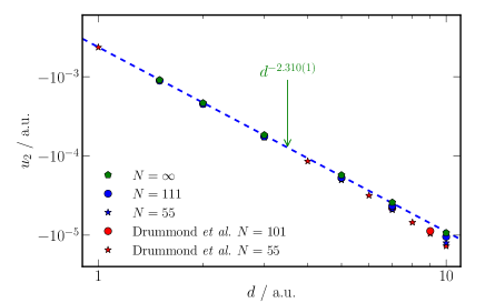
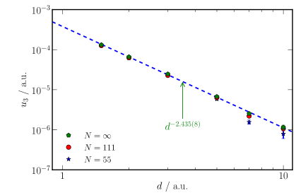
Figure 5: DMC results for the asymptotic behaviour of the biwire interaction $u_{2}$ (left panel) and the nonadditive triwire contribution $u_{3}$ (right panel) at $r_{s}=1$.

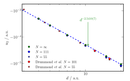
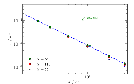
Figure 6: DMC results for the asymptotic behaviour of the biwire interaction $u_{2}$ (left panel) and the nonadditive contribution $u_{3}$ (right panel) at $r_{s}=3$.

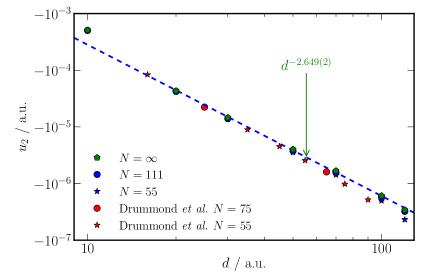
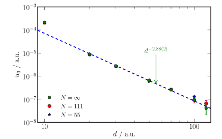
Figure 7: DMC results for the asymptotic behaviour of the biwire interaction $u_{2}$ (left panel) and the non-additive contribution $u_{3}$ (right panel) at $r_{s}=10$.

To estimate the finite-size errors at a given wire separation $d$, we examined the variation of the energy with the number $N$ of electrons per wire. It has recently been reported Lee and Drummond (2011) that the finite-size error in the total energy per electron of the 1D HEG scales as

$$e_{1}(N)=e_{1}(\infty)+\frac{c}{N^{2}},$$ (17)

where $c$ is a constant, over the range of $N$ considered here. Our results for $e_{2}$ and $e_{3}$, shown in Fig. 8, are consistent with this dependence. However, we find that the interaction energies $u_{2}$ and $u_{3}$ at a given $d$ show a more slowly decaying finite-size error:

$$u_{M}\left(N\right)=u_{M}(\infty)+\frac{c^{\prime}}{N},$$ (18)

where $c^{\prime}$ is a constant. Hence Eq. (17) cannot give the asymptotic form of the finite-size error in the total energy of a 1D system in the limit of large $N$.

We have extrapolated the binding-energy data shown in Figs. 5–7 to the thermodynamic limit at each $d$ using Eq. (18). We have then fitted Eq. (16) to the extrapolated binding-energy data for triwires and biwires, respectively. The resulting fitting parameters, including the asymptotic exponents, are given in Table 1.

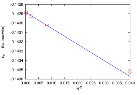
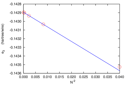
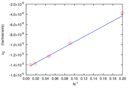
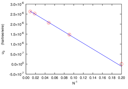
Figure 8: DMC results for the $N$-dependence of the total biwire ($e_{2}$) and triwire ($e_{3}$) energies and interaction energies ($u_{2}$ and $u_{3}$) at $r_{s}=10$ and at interwire spacing $d=30$ a.u. The data at $N=5$ ($1/N=0.2$, $1/N^{2}=0.04$) were excluded from the fits (solid lines).

Table 1: Values of power-law parameters in Eq. (16) for the two-body and three-body energies.

	$u_{2}\mathchar 12604\relax 0$			$u_{3}\mathchar 12606\relax 0$
	$C$	$\alpha$		$C$	$\alpha$
$r_{s}=1$	$-6\cdot 0685(6)$	$2\cdot 310(1)$		$-7\cdot 942(5)$	$2\cdot 435(8)$
$r_{s}=3$	$-4\cdot 084(1)$	$2\cdot 5410(7)$		$-5\cdot 565(8)$	$2\cdot 670(5)$
$r_{s}=10$	$-2\cdot 114(6)$	$2\cdot 649(2)$		$-2\cdot 98(5)$	$2\cdot 88(2)$

IV Discussion

We have investigated the nature of the non-additive dispersion between three parallel wires and we have demonstrated that as the HOMO–LUMO gap (band gap in infinite wires) decreases, the deviations of $E^{(3)}_{\rm disp}[3]$ from the conventional triple-dipole Axilrod–Teller–Muto model increase. These deviations occur mainly in two ways:

• For wire separations smaller than the typical electron correlation length, the effective three-body non-additive dispersion behaves as $u_{3}(d)\sim d^{-\beta}$, where $\beta\rightarrow 3$ as the HOMO–LUMO gag decreases. This power-law arises from the correlations between extended charge fluctuations that are associated from the plasmon-like modes in the wires. This is a substantially slower decay than the $u_{3}(d)\sim d^{-7}$ behaviour expected from the standard triple-dipole summations associated with local dipole fluctuations. For finite wires, $u_{3}(d)\sim d^{-9}$ for separations much larger than the wire length.

• $u_{3}(d)$ is substantially enhanced as the gap reduces. This is most dramatic for large separations, where we observed an enhancement of four orders of magnitude for the near-metallic wires compared with the wires with the largest HOMO–LUMO gap.

These observations are analogous to those obtained by Misquitta et al. Misquitta et al. (2010) with regard to the second-order dispersion energy $E^{(2)}_{\rm disp}$, though the effects of metallicity are more dramatic for the three-body non-additivity. We have provided a simple physical picture of correlations in extended charge fluctuations using which both of these observations can be understood.

We have established these results using two techniques: (1) a generalised multipole expansion for $E^{(3)}_{\rm disp}[3]$ that includes contributions from charge-flow polarizabilities responsible for the long-wavelength, plasmon-like fluctuations, and (2) DMC. The former has the advantage that we can directly calculate $E^{(3)}_{\rm disp}[3]$, but it is applicable only to finite systems with non-zero HOMO–LUMO gaps. By contrast, DMC is applicable to infinite systems (modelled in cells subject to periodic boundary conditions) with zero gaps, and in principle is able to describe the third-order correlation energy exactly. However, like any supermolecular technique, that is, techniques that calculate the interaction energy from total energy differences, DMC is unable to separate the two-body energy $E^{(3)}_{\rm disp}[2]$ from the three-body non-additive dispersion $E^{(3)}_{\rm disp}[3]$. Nevertheless, there is a consistency in the results from these two methods. At short range (i.e., at separations less than the correlation length) the multipole expansion used on trimers of finite (H₂)₆₄ chains yields a power-law of $u_{3}(d)\sim d^{-\beta}$ where $\beta\rightarrow 3^{+}$, that is, $\beta$ approaches $3$ from above, while in the DMC results, $\beta\rightarrow 3^{-}$ as $r_{s}$ increases. For small $r_{s}$ the exponent is significantly smaller than $3$. This could be because of finite-size effects, contributions from $E^{(3)}_{\rm disp}[2]$, or it could be a genuine effect not captured by the multipole expansion.

The increased effect of the plasmon-like, charge-flow fluctuations on $E^{(3)}_{\rm disp}[3]$ compared with $E^{(2)}_{\rm disp}$ is related to the long range of these fields produced by the fluctuations. The dipole fluctuations in insulators result in electric fields that behave as $r^{-3}$; a rapid decay compared with the $r^{-1}$ behaviour of the electric fields from the plasmon-type fluctuations. Consequently we expect the many-body expansion to be slowly convergent for conglomerates of low-dimensional semi-metallic systems. As we have demonstrated, the three-body non-additivity quenches the already enhanced two-body dispersion. Likewise, by extending our physical model for these anomalous dispersion effects, we expect that the four-body non-additivity will be attractive and decay as $-d^{-4}$ for 1D metallic systems, and will consequently quench the three-body non-additivity.

The slow decay and alternating signs of the $N$-body non-additive dispersion suggests that the many-body expansion may not be a useful way of modelling the dispersion interaction in, say, a bundle of 1D semi-metallic wires. An alternative may be a generalisation of the self-consistent polarization model proposed by Silberstein Silberstein (1917) and Applequist Applequist et al. (1972), and recently significantly developed by Tkatchenko et al. Tkatchenko et al. (2012). However, models such as these would have to be modified to include the charge-flow polarizabilities to be able to describe the metallic effects described in this article.

For finite molecular systems, the changes in power-law described here are, to an extent, of academic interest only. In practice, subtle power-law changes in the dispersion interaction can be easily masked by the other, often larger, components of the interaction energy, particularly the first-order electrostatic energy. While this may be the case, it is the second effect—the enhancement of the dispersion energy that arises from the plasmon-like modes—that may have a perceptible effect. The long-wavelength fluctuations cause an enhancement of the effective two- and three-body dispersion coefficients. We believe that this effect, which is captured by techniques such as the Williams–Stone–Misquitta methodMisquitta and Stone (2008); Misquitta et al. (2008), may prove significant even for relatively small molecular systems. We are currently working to investigate this phenomenon.

V Acknowledgments

Financial support was provided by the UK Engineering and Physical Sciences Research Council (EPSRC). Part of the computations have been performed using the K computer at Advanced Institute for Computational Science, RIKEN. R.M. is grateful for financial support from KAKENHI grants (23104714, 22104011, and 25600156), and from the Tokuyama Science Foundation.

References

- Spencer (2009) J. Spencer, Ph.D. thesis, St. Catharine’s College, University of Cambridge (2009).
- Misquitta et al. (2010) A. J. Misquitta, J. Spencer, A. J. Stone, and A. Alavi, Phys. Rev. B 82, 075312 (2010).
- Drummond and Needs (2007) N. D. Drummond and R. J. Needs, Phys. Rev. Lett. 99, 166401(4) (2007).
- Dobson et al. (2006) J. F. Dobson, A. White, and A. Rubio, Phys. Rev. Lett. 96, 073201(4) (2006).
- Stone (2013) A. J. Stone, The Theory of Intermolecular Forces (Oxford University Press, Oxford, 2013), 2nd ed.
- Kaplan (2005) I. G. Kaplan, Intermolecular Interactions (Wiley, 2005), 2nd ed.
- Foulkes et al. (2001) W. M. C. Foulkes, L. Mitas, R. J. Needs, and G. Rajagopal, Rev. Mod. Phys. 73, 33 (2001), URL http://link.aps.org/doi/10.1103/RevModPhys.73.33.
- Dobson (2007) J. F. Dobson, Surface Science 601, 5667 (2007).
- Dobson et al. (2001) J. F. Dobson, K. McLennan, A. Rubio, J. Wang, T. Gould, H. M. Le, and B. P. Dinte, Aust. J. Chem. 54, 513 (2001).
- Coulson and Davies (1952) C. A. Coulson and P. L. Davies, Trans. Faraday Soc. 48, 777 (1952).
- Longuet-Higgins and Salem (1961) H. C. Longuet-Higgins and L. Salem, Proc. R. Soc. A 259, 433 (1961).
- Chang et al. (1971) D. B. Chang, R. L. Cooper, J. E. Drummond, and A. C. Young, Phys. Lett. 37A, 311 (1971).
- Gobre and Tkatchenko (2013) V. V. Gobre and A. Tkatchenko, Nature Communications 4, 2341 (2013).
- Misquitta and Stone (2008) A. J. Misquitta and A. J. Stone, J. Chem. Theory Comput. 4, 7 (2008).
- Misquitta et al. (2008) A. J. Misquitta, A. J. Stone, and S. L. Price, J. Chem. Theory Comput. 4, 19 (2008).
- Angyan (2009) J. G. Angyan, Int. J. Quantum Chem. 109, 2340 (2009).
- Parsegian (2005) V. A. Parsegian, Van der Waals Forces: A Handbook for Biologists, Chemists, Engineers, and Physicists (Cambridge University Press, 2005).
- Stogryn (1971) D. E. Stogryn, Mol. Phys. 22, 81 (1971).
- Axilrod and Teller (1943) P. M. Axilrod and E. Teller, J. Chem. Phys. 11, 299 (1943).
- Muto (1943) Y. Muto, Proc. Phys.-Math. Soc. Japan 17, 629 (1943).
- Longuet-Higgins (1965) H. C. Longuet-Higgins, Disc. Faraday Soc. 40, 7 (1965), spiers Memorial Lecture.
- Stone (1985) A. J. Stone, Mol. Phys. 56, 1065 (1985).
- Misquitta and Stone (2006) A. J. Misquitta and A. J. Stone, J. Chem. Phys. 124, 024111 (2006).
- Le Sueur and Stone (1994) C. R. Le Sueur and A. J. Stone, Mol. Phys. 83, 293 (1994).
- Lillestolen and Wheatley (2007) T. C. Lillestolen and R. J. Wheatley, J. Phys. Chem. A 111, 11141 (2007).
- Sadlej (1988) A. J. Sadlej, Coll. Czech Chem. Commun. 53, 1995 (1988).
- Bylaska et al. (2006) E. J. Bylaska, W. A. de Jong, K. Kowalski, T. P. Straatsma, M. Valiev, D. Wang, E. Apra, T. L. Windus, S. Hirata, M. T. Hackler, et al., NWChem, a computational chemistry package for parallel computers, version 5.0, Pacific Northwest National Laboratory, Richland, Washington 99352-0999, USA. (2006).
- Misquitta and Stone (2013) A. J. Misquitta and A. J. Stone, CamCASP: a program for studying intermolecular interactions and for the calculation of molecular properties in distributed form, University of Cambridge (2013), http://www-stone.ch.cam.ac.uk/programs.html#CamCASP. Accessed: Oct 2013.
- Champagne et al. (1998) B. Champagne, E. A. Perpete, S. J. A. van Gisbergen, E.-J. Baerends, J. G. Snijders, C. Soubra-Ghaoui, K. A. Robins, and B. Kirtman, J. Chem. Phys. 109, 10489 (1998).
- Champagne et al. (1995a) B. Champagne, D. H. Mosley, M. Vracko, and J.-M. Andre, Phys. Rev. A 52, 178 (1995a).
- Champagne et al. (1995b) B. Champagne, D. H. Mosley, M. Vracko, and J.-M. Andre, Phys. Rev. A 52, 1039 (1995b).
- Saunders et al. (1994) V. R. Saunders, C. Freyria-Fava, R. Dovesi, and C. Roetti, Comp. Phys. Commun. 84, 156 (1994).
- Drummond et al. (2004) N. D. Drummond, M. D. Towler, and R. J. Needs, Phys. Rev. B 70, 235119(11) (2004).
- Lopez Rios et al. (2006) P. Lopez Rios, A. Ma, N. D. Drummond, M. D. Towler, and R. J. Needs, Phys. Rev. E 74, 066701 (2006), URL http://link.aps.org/doi/10.1103/PhysRevE.74.066701.
- Lee and Drummond (2011) R. M. Lee and N. D. Drummond, Phys. Rev. B 83, 245114 (2011), URL http://link.aps.org/doi/10.1103/PhysRevB.83.245114.
- Needs et al. (2010) R. J. Needs, M. D. Towler, N. D. Drummond, and P. L. Rios, J. Phys.: Condens. Matter 22, 023201(15) (2010).
- Trail (2008) J. R. Trail, Phys. Rev. E 77, 016703 (2008), URL http://link.aps.org/doi/10.1103/PhysRevE.77.016703.
- Trail and Maezono (2010) J. R. Trail and R. Maezono, The Journal of Chemical Physics 133, 174120 (pages 16) (2010), URL http://link.aip.org/link/?JCP/133/174120/1.
- Silberstein (1917) L. Silberstein, Phil. Mag. 33, 92 (1917).
- Applequist et al. (1972) J. Applequist, J. R. Carl, and K.-K. Fung, J. Am. Chem. Soc. 94, 2952 (1972).
- Tkatchenko et al. (2012) A. Tkatchenko, R. A. DiStasio, R. Car, and M. Scheffler, Phys. Rev. Lett. 108, 236402 (2012), URL http://link.aps.org/doi/10.1103/PhysRevLett.108.236402.