Impossibility of strict thermodynamic equilibrium establishment in the accelerated Universe

Abstract

In this article there are considered non-equilibrium cosmological scenarios with the assumption that scaling of particles interaction is restored in range of extra-high energies. On basis of energy-balance equation’s exact solutions it is obtained the strong conclusion about fundamental unattainability of local thermodynamic equilibrium in the accelerated Universe. There are presented the results of numerical simulation of previously constructed strict mathematical model which describes thermodynamic equilibrium’s establishment in the originally nonequilibrium cosmological ultrarelativistic plasma for the Universe with an arbitrary acceleration with the assumption that scaling of interactions of elementary particles is restored at energies above the unitary limit. Limiting parametres of residual nonequilibrium distribution of extra-high energy relic particles are obtained. The assumption about possibility of detection of ”truly relic particles”, which appeared at stage of early inflation, is put forward.

Keywords: physics of the early universe, particle physics - cosmology connection, inflation, ultra high energy cosmic rays

1 Conditions for the local thermodynamic equilibrium of cosmological plasma

One of the main statements of the standard cosmological scenario (SCS) is an assumption of local thermodynamic equilibrium (LTE) of cosmological plasma on the early stage of Universe expansion. As is known, to let LTE establish in the statistical system, it is required that the effective time between particles collisions, $\tau_{eff}$, is small as compared to the typical time scale of system evolution. In the cosmological situation such scale is Universe age, and more precisely, inverse value of the scale factor’s $a(t)$ logarithmical derivative. This brings us to the following well-known LTE condition in the expanding ultrarelativistic cosmological plasma:

$$\frac{\dot{a}}{a}\tau_{eff}\ll 1,\Rightarrow\frac{\dot{a}}{a}\frac{1}{n(t)\sigma_{tot}}\ll 1,$$ (1)

where $a(t)$ is a scale factor, $\dot{a}\equiv da/dt$, $n(t)$ is a particles number density, $\sigma_{tot}$ is a total cross-section of particles scattering in pair collisions.

1.1 Kinematics of four-particles collisions

Four-particles reactions of type

$$a+b\rightarrow c+d.$$ (2)

are fully described by two kinematic invariants, $s$ and $t$ (see, e.g. [2]):

$$s=(p_{a}+p_{b})^{2}\equiv(p_{a}+p_{b},p_{a}+p_{b}),$$ (3)

colliding particles’ square energy in the center-of-mass system, and

$$t=(p_{c}-p_{a})^{2}=(p_{b}-p_{d})^{2}.$$ (4)

the relativistic square of the transmitted momentum:. Next, $(p,q)\equiv g_{ik}p^{i}q^{k}$ is a scalar product of vectors $p,q$ relative to metric $g$, $a,b$ are particles indexes, $i,k=\overline{1,4}$; $\sqrt{s}$ is an energy of colliding particles in the center-of-mass system (CMS).

Invariant scattering amplitudes are determined as a result of invariant scattering amplitude averaged by “$c$” and “$d$” particles’ states at that are turned out to be dependent only on these two invariants:

$$\overline{|M_{FJ}|^{2}}=|F(s,t)|^{2},$$ (5)

where $S_{i}$ are particles spins. Total cross-section of the reaction (2) is determined by means of the invariant amplitude $F(s,t)$:

$$\sigma_{tot}=\frac{1}{16\pi\lambda(s,m^{2}_{a},m^{2}_{b})}\int\limits_{t_{min}}^{t_{max}}dt|F(s,t)|^{2},$$ (6)

where $m_{i}$ are particles rest masses, $\lambda$ is a triangle function:

$$\lambda^{2}(a,b,c)=a^{2}+b^{2}+c^{2}-2ab-2ac-2bc,$$

$$t^{\rm max}_{\rm min}=\frac{4}{s}[(m^{2}_{c}-m^{2}_{a}+m^{2}_{b}-m^{2}_{d})^{2}-(\sqrt{\lambda}\mp\sqrt{\lambda^{\prime}})^{2}],$$

where the following denotations are introduced for the simplicity:

$$\lambda=\lambda(s,m^{2}_{a},m^{2}_{b});\;\lambda^{\prime}=\lambda(s,m^{2}_{c},m^{2}_{d}).$$

In the ultrarelativistic limit

$$\frac{p_{i}}{m_{i}}\to\infty$$ (7)

we have:

$$s\rightarrow 2(p_{a},p_{b}); t\rightarrow-2(p_{a},p_{b}); \lambda\to s^{2};$$

$$t_{min}=\rightarrow-s; t_{max}\rightarrow 0; \frac{s}{m^{2}_{i}}\to\infty,$$

and formula (6) is significantly simplified by the introduction of the dimensionless variable:

$$x=-\frac{t}{s}:$$ (8)

$$\sigma_{tot}(s)=\frac{1}{16\pi s}\int\limits_{0}^{1}dx|F(s,x)|^{2}.$$ (9)

Thus, total cross-section of scattering depends only on kinematic invariant $s$ - square energy of colliding particles in the center-of-mass system:

$$\sigma_{tot}=\sigma_{tot}(s).$$ (10)

Exactly this dependency controls LTE establishment in the early Universe.

1.2 Influence of $\sigma(s)$ on the process of LTE restoration

In the space-flat Friedmann metric which is considered in the article,

$$ds^{2}=dt^{2}-a^{2}(t)(dx^{2}+dy^{2}+dz^{2})$$ (11)

integral of motion is a conformal momentum (see e.g. [3])

$$\tilde{p}=a(t)p={\rm const},$$ (12)

where $p=\sqrt{-g_{\alpha\beta}p^{\alpha}p^{\beta}}$ is a physically three-dimensional momentum ($\alpha,\beta=\overline{1,3}$) $a$ is a scale factor. Thus, for ultrarelativistic particles

$$s\sim p^{2}\sim a^{-2}.$$ (13)

Assuming power dependence of total particles cross-section on $s$

$$\sigma_{tot}\sim s^{\nu}$$ (14)

and barotropic summary equation of matter state ${\rm p}=\varkappa\varepsilon$, where ${\rm p}$ is a summary pressure , $\varepsilon$ is a summary energy density, $\varkappa$ is a barotrope factor, under the assumption of total particles number conservation $n(t)a^{3}(t)={\rm const}$ we arrive to the following conclusion [5].

Statement 1

At fulfillment of the condition

$$4\nu+3(1-\varkappa)>0;\quad(\varkappa\not=-1),$$ (15)

LTE is maintained on early stages of expansion and is broken on the late ones, i.e., at:

$$\nu>-\frac{3}{4}(1-\varkappa)\Rightarrow\;LTE\;\mbox{\rm at}\;t<t_{0},$$ (16)

and at fulfillment of the inverse to (16) condition LTE is broken on early stages and is restored at late ones $t>t_{0}$.

In particular,
$1^{0}$. in case of ultrarelativistic equation of state $\varkappa=1/3$ we obtain from (16) the condition of LTE existence on early stages of expansion [5] —

$$\nu>-\frac{1}{2}\Rightarrow\;LTE\;\mbox{\rm at}\;t<t_{0},\quad p=\frac{1}{3}\varepsilon;$$ (17)

$2^{0}$. in case of utmost rigid equation of state $\varkappa=1$ condition of LTE maintenance on early stages and breaking on late stages is equivalent to the condition

$$\nu>0\Rightarrow\;LTE\;\mbox{\rm at}\;t<t_{0},\quad(p=\varepsilon)$$ (18)

(hence it follows that at constant cross-section of scattering $\nu=0$ in case of utmost rigid equation of state time is completely excluded from the condition of LTE [5], - at this stage of expansion in the Universe LTE either exists at all times or always is absent.);
$3^{0}$. in case of inflation $\varkappa=-1$ at fulfillment of the condition

$$\nu>-\frac{3}{2}$$ (19)

LTE is maintained at early stages ($t<t_{0}$) and is broken on late ones ($t>t_{0}$). The last is obviously true at conservation of the total particles number at the inflationary stage of expansion.

2 Unified asymptotic cross-section of scattering

2.1 Unitarity and unitary limit

For the investigation of the early Universe processes’ kinetics it is required to know an asymptotic behavior of the invariant amplitudes$F(s,t)$ in the limit (7). Modern experimental possibilities are limited by values $\sqrt{s}$ of the order of several Tev. It would be incautious to bear on one or another field interaction model for the forecasting of the asymptotic behavior of the scattering cross-section in range of extra-high energies of the order of $10^{11}\div 10^{16}$ Tev. At modern conditions it looks more reasonable to bear on the conclusions of the asymptotic theory of $S$-matrix, which are obtained on the basis of fundamental laws of unitarity, causality, scale invariance etc. The unitarity of the $S$-matrix leads to the well-known asymptotic relation (see e.g. [6]):

$$\left.\frac{d\sigma}{dt}\right|_{s\to\infty}\sim\frac{1}{s^{2}}$$ (20)

at value of $s$ above the unitary limit, i.e under the condition (7), if by $m_{i}$ we understand masses of all intermediate particles. However then from (9) it follows:

$$F(s,1)|_{s\to\infty}\sim\mbox{Const}.$$ (21)

Conception of the unitary limit was first introduced by L.D. Landau in 1940 for vector mesons [7]. Following that article, by unitary limit energy we understand such a critical energy, above the value of which the growth of the effective cross-section of scattering is stopped and its behavior obeys the condition of unitarity. For example, for the standard $\nu e$ - scattering the energy of the unitary limit $E_{u}=\sqrt{s_{u}}$ is (see e.g. [6]) $\sqrt{\sqrt{2}\pi/G_{\nu}}$ $\approx 600$ Gev, where $G_{\nu}$ is an electroweak interaction constant.

2.2 Asymptotic behavior of particles scattering cross-sections in range of extra-high energies

On the basis of the axiomatic theory of the $S$ - matrix in 60’s there were obtained strict limitations on the asymptotic behavior of the total cross-sections of scattering and its invariant amplitudes:

$$\frac{C_{1}}{s^{2}\ln s}<\sigma_{tot}(s)<C_{2}\ln^{2}s,$$ (22)

where $C_{1},C_{2}$ are unknown constants. The upper limit (22) has been determined in articles [8], [9], [10], the lower one - in articles [11], [12], see also a review in the book [13]. Let us also point out limitations on the invariant amplitudes of scattering [13]:

$$|F(s,t)|\leq|F(s,0)|;$$ (23)

$$C^{\prime}_{1}<|F(s,0)|<C^{\prime}_{2}s\ln^{2}s.$$ (24)

Thus invariant amplitudes of scattering in the limit (7) must be functions of only one variable $x=-t/s$, i.e.:

$$|F(s,t)|=|F(x)|,\;(s\to\infty).$$ (25)

However then as a result of (9)

$$\sigma_{tot}(s)=\frac{1}{16\pi s}\int\limits_{0}^{1}dx|F(x)|^{2}=\frac{\mbox{Const}}{s}$$ (26)

— the total cross-section’s behavior is the same as for the electromagnetic interactions, i.e. at extra-high energies, scaling is restored.

Scaling asymptotics of scattering (26) lies strictly in the middle of possible extreme asymptotics of total scattering cross-section (22). Moreover, if (26) is fulfilled, relations (20) and (21) obtained on the basis of the axiomatic theory of the $S$ - matrix are also automatically fulfilled

For the lepton-hadron interaction a suggestion of scaling existence has been put forward in articles [14], [15], [16]. In particular, for the total cross-section of the reaction ”$e+e^{+}\rightarrow\mbox{hadrons}$” an expression has been obtained:

$$\sigma_{tot}=\frac{4\pi\alpha^{2}}{3s}\sum e^{2}_{i},$$

where $\alpha$ is a fine structure constant, $e_{i}$ are charges of fundamental fermion fields. The data obtained on the Stanford collider, confirmed scaling existence for these interactions. For the gravitational interactions scaling, apparently, should be restored at extra-high energies in consequence of the scale invariance of the gravitational interactions in WKB-approach [17]. There can be made a lot of similar examples which are reliable established facts.

2.3 Universal asymptotic cross-section of
scattering

Let us hereinafter suggest the existence of scaling at energies above the unitary limit $s\to\infty$. Then the question about the meaning of the constant in formula (26) and also about the logarithmic refinement of this constant arises. This value can be estimated from the following simple considerations. First, let $m$ be a rest mass of the colliding particles. Since $\sqrt{s}$ is an energy of the interacting particles in the center-of-mass system, the minimum value $\sqrt{s}$ for the four-particles reactions with the particles of mass $m$ is:

$$\sqrt{s_{\rm min}}=2m\Rightarrow s_{\rm min}=4m^{2}.$$ (27)

Next, if the idea about unification of all interactions on Planck energy scales $E_{pl}=m_{pl}=1$ is correct, then at $s\sim 1$ all four-particle interactions must be described by the single cross-section of scattering, that is formed of three fundamental constants $G,\hbar,c$, i.e., in the chosen system of units it should be:

$$\sigma|_{s\sim 1}=2\pi l^{2}_{pl}\Rightarrow\sigma(4)=\frac{8\pi}{s_{pl}}\quad(=2\pi),$$ (28)

where:

$$s_{pl}=4m^{2}_{pl}=4$$ (29)

is a Planck value of the kinematic invariant $s$ corresponding to two colliding plankeons with mass $m_{pl}$ and Compton scale $l_{pl}$:

$$m_{pl}=\sqrt{\frac{\hbar c}{G}}\;(=1),\quad l_{pl}=\sqrt{\frac{G\hbar}{c^{3}}}\;(=1).$$ (30)

However, in order to decrease to such value on Planck energy scales, starting from values of order $\sigma_{T}=8\pi\alpha^{2}/3m^{2}_{e}$ ($m_{e}$ - electron mass, $\sigma_{T}$ - Thompson cross-section of scattering) for the electromagnetic interactions, i.e. at $s\sim 4m^{2}_{e}$, cross-section of scattering should decrease in inverse proportion to $s$, i.e. again by scaling law. Let us note that this fact is one more independent argument in favor of existence of scaling in range of extra-high energies. Refining this dependency logarithmically we introduce the universal asymptotic cross-section of scattering (ACS), which first was proposed in articles [4] (1984), [5], (see also [18]):

$$\sigma_{0}(s)=\frac{8\pi\beta}{sL(s)},$$ (31)

where $\beta\sim 1$, $L(s)$ is a logarithmical factor:

$$L(s)=1+\ln^{2}\left(1+\frac{s_{0}}{s}\right)>1,$$ (32)

which is a monotone decreasing function of the kinematic invariant $s$: $dL/ds<0,$ and $s_{0}=4$ is a squared total energy of two colliding Planck masses so that on Planck energy scales:

$$L(s_{0})\simeq 1,$$ (33)

at that on Compton scales of energy, i.e. at $s=m^{2}_{e}$:

$$\frac{1}{\sqrt{L(m^{2}_{e})}}\approx\frac{1}{102}\simeq\alpha\approx\frac{1}{137},$$ (34)

where $\alpha=1/137$ is a fine structure constant.

Relation (34) allows to consider value $1/\sqrt{L(s)}$ as logarithmically changing effective constant of interaction, which, in its turn, realizes the ideology of running interaction constants of standard theories of $SU(5)$ - type fundamental interactions.

Introduced by formual (31), cross-section of scattering $\sigma_{0}$, ACS, possesses a number of remarkable features (see also Figure 2.3):
$1^{o}$. ACS is formed with a use of only fundamental constants $G,\hbar,c$;
$2^{o}$. ACS behaves itself so that its values lie strictly in the middle of possible extreme limits of the asymptotic behavior of cross-section (22), which were established by means of the asymptotic theory of the $S$-matrix;
$3^{o}$. With logarithmic accuracy ACS is a scaling cross-section of scattering ;
$4^{o}$. ACS with a remarkable accuracy coincides with cross-sections of all known fundamental processes on the corresponding energy scales, starting from the electromagnetic and finishing with gravitational ones on the huge range of energy values (from $m_{e}$ to $10^{22}m_{e}$) — the values of the first kinematic invariant at that changes by an order of of 44!! (see Figure 2.3).
In the previous works there were given the arguments in favor of scaling behavior of the scattering cross-section in range of energy above the unitary limit. Among them there was provided the comparison of ACS with the specific cross-sections of scattering for certain specific four-particle reactions at the corresponding energy ranges. However, during the discussions with experts in the quantum field theory the unacceptance of the statement about scaling behavior of the scattering cross-section is often found out. The Author suggests that this unacceptance is caused, first of all, by quite limited range of energies for which the calculations of concrete scattering cross-sections are carried out, and second, by the “look from below” on quantum procedures of calculation of scattering cross-sections in sense that energy is considered below the unitary limit. For elimination of this misunderstanding” in this article Author represents the comparison of the asymptotic scattering cross-section’s values (31) with the known quantum four-partial processes in the graphic format (Figure 2.3).

Figure 1.     Comparison of the universal cross-section of scattering (31) at factor $\beta=1$ with the well-known cross-sections of fundamental processes is noted by bold line. Dotted line corresponds to the graph of universal cross-section of scattering at factor $\beta=2$. On the abscissa axis are laid values of the common logarithm of the first kinematic invariant $\lg s$ in Planck units; along the ordinate axis are laid values of the common logarithm of the dimensionless invariant, $\lg s\sigma(s)$. 1 – Thompson scattering, 2 – Compton scattering on electrons at $E_{SCM}=10$ Mev, 3 – Compton scattering of electrons at $E_{SCM}=1$ Gev, 4 – electroweak interaction with participation of: $W$ - bosons, 5 – with participation of $Z$ - bosons, 6 – with participation of H-bosons at energy of the order of 7 Tev ($\sigma\sim 10$fb); 7 – $SU(5)$ - interaction at mass of the superheavy X-bosons $10^{15}$ Gev, 8 – $10^{14}$ Gev; 9 – gravitational interaction on Planck scales. Vertical dotted lines correspond to energy values of the unitary limit for $SU(2)\times SU(1)$ - interactions, $E_{u}=617$ Gev, and SU(5) - interactions, $E_{u}\sim 10^{14}$ Gev.

These remarkable properties of ACS hardly can be accidental and allow us further use ACS as a reliable formula for the asymptotic value of scattering cross-sections for all interactions.

3 Kinetic equations for superthermal particles

3.1 Simplification of relativistic collision integral

Process of thermodynamic equilibrium establishment is described by relativistic kinetic equations. In paper [3] it is shown that relativistic kinetic equations are conformally invariant in ultrarelativistic limit at existence of scaling of interactions. This fact is the basis for the assertion that at least in the ultrarelativistic Universe LTE could be broken. So, we consider homogenous isotropic distributions of particles in Friedmann metric (11). Such distributions are described by functions:

$$f_{a}(x^{i},p^{k})=f_{a}(t,p).$$ (35)

Relativistic kinetic equations relatively to homogenous isotropic distributions (35) take form (details see in [19], [20], [21], [22], [23]):

$$\frac{\partial f_{a}}{\partial t}-\frac{\dot{a}}{a}p\frac{\partial f_{a}}{\partial p}=\frac{1}{\sqrt{m_{a}^{2}+p^{2}}}\sum\limits_{b,c,d}J_{ab}(t,p),$$ (36)

where $J_{ab}(t,p)$ -is an integral of 4-particle reactions [23], [21]:

$$J_{ab}(t,p)=(2\pi)^{4}\int d\pi_{b}d\pi_{c}d\pi_{d}\delta^{(4)}(p_{a}+p_{b}-p_{c}-p_{d})$$ (37)

$$\times[(1\pm f_{a})(1\pm f_{b})|f_{c}f_{d}\overline{|M_{cd\to ab}|^{2}}-(1\pm f_{c})(1\pm f_{d})f_{a}f_{b}|\overline{M_{ab\to cd}|^{2}}\,],$$

signs $\pm$ correspond to bosons ($+$) and fermions ($-$), $M_{i\to f}$ are invariant scattering amplitudes (underscore means averaging by particles’ polarization states), $d\pi_{a}$ is a normalized volume element of momentum space of $a$-particle:

$$d\pi_{a}=\sqrt{-g}\frac{\rho_{a}dp^{1}dp^{2}dp^{3}}{(2\pi)^{3}p_{4}},$$ (38)

$\rho_{a}$ - degeneration factor.

Let us simplify the integral of 4-particle interactions (3.1), using properties of distributions $f_{a}(t,p)$ isotropy. For the fulfillment of two inner integrations by momentum variables we pass to the local center-of-mass system, where integration is carried out very simply. After the inverse Lorentz transform and proceed to the spherical coordinate system in the momentum space in the ultrarelativistic limit (7) we find ([5], [24]):

$$J_{ab}(p)\!\!=\!\!-{\displaystyle\frac{2S_{b}+1}{(2\pi)^{3}p}}{\displaystyle\int\limits_{0}^{\infty}}\!dq{\displaystyle\int\limits_{0}^{4pq}\!\!\frac{ds}{16\pi}}{\displaystyle\int\limits_{0}^{1}}dx|F(x,s)|^{2}{\displaystyle\int\limits_{0}^{2\pi}}\!\!d\varphi\times$$

$$\{f_{a}(p)f_{b}(q)[1\pm f_{c}(p-\Delta)][1\pm f_{d}(q+\Delta)]$$

$$-f_{c}(p-\!\!\Delta)f_{d}(q+\!\!\Delta)[1\pm\!\!f_{a}(p)][1\pm\!\!f_{b}(q)]\},$$ (39)

where $x=-t/s$ dimensionless variable (8), and

$$\Delta=x(p-q)-\cos\varphi\sqrt{x(1-x)(4pq-s)}.$$ (40)

3.2 Relativistic kinetic equations in terms of conformally corresponding space

Taking into account the fact that variable $\tilde{p}$ (12) is an integral of motion in Friedmann metric and at that for any function $\Psi(t,p)$ holds the relation [19]:

$$\frac{\partial\Psi(t,p)}{\partial t}-\frac{\dot{a}}{a}p\frac{\partial\Psi(t,p)}{\partial p}=\frac{\partial\Psi(t,\tilde{p})}{\partial t},$$ (41)

we transform the kinetic equations for the homogenous isotropic distributions to the form:

$$\frac{\partial f_{a}}{\partial\eta}=\frac{a}{\sqrt{m_{a}^{2}+p^{2}}}\sum\limits_{b,c,d}J_{ab}(\eta,p),$$ (42)

where it is necessary to substitute $p=\tilde{p}/a$.

Let us note that from the other hand, transformation to varaible (12), $\tilde{p}$, is practically a conformal transformation to the homogenous static space

$$ds^{2}=a^{2}ds_{0}^{2}=a^{2}(d\eta^{2}-dl^{2}),$$

where physical component of the momentum, $p$, is transformed by the law:

$$p=\frac{\tilde{p}}{a}.$$ (43)

Thus, the momentum variable (12), $\tilde{p}$, is an absolute magnitude of the physical momentum in the conformally corresponding static space of constant curvature, and $\eta$ is a time variable in this space.

Particles number densities, $n(\eta)$, and their energy densities, $\varepsilon(\eta)$, relatively to the isotropic particles distribution, $f(\eta,p)$ are determined by formulas):

$$n(\eta)={\displaystyle\frac{\rho}{2\pi^{2}}\int\limits_{0}^{\infty}}p^{2}f(\eta,p)dp={\displaystyle\frac{\rho}{2\pi^{2}a^{3}}\int\limits_{0}^{\infty}}\tilde{p}^{2}f(\eta,\tilde{p})d\tilde{p};$$ (44)

$$\begin{array}[]{l}\varepsilon(\eta)={\displaystyle\frac{\rho}{2\pi^{2}}\int\limits_{0}^{\infty}}\sqrt{m^{2}+p^{2}}p^{2}f(\eta,p)dp=\\ ={\displaystyle\frac{\rho}{2\pi^{2}a^{3}}\int\limits_{0}^{\infty}}\tilde{p}^{2}\sqrt{m^{2}+\tilde{p}^{2}/a^{2}}f(\eta,\tilde{p})d\tilde{p}.\end{array}$$ (45)

In connection with this it is convenient to introduce conformal particles number densities, $\tilde{n}(\eta)$, and for the ultrarelativistic particles also their energy densities, $\tilde{\varepsilon}(\eta)$:

$$\tilde{n}(\eta)={\displaystyle\frac{\rho}{2\pi^{2}}\int\limits_{0}^{\infty}}\tilde{p}^{2}f(\eta,\tilde{p})d\tilde{p};$$ (46)

$$\tilde{\varepsilon}(\eta)={\displaystyle\frac{\rho}{2\pi^{2}}\int\limits_{0}^{\infty}}\sqrt{m^{2}+p^{2}}p^{2}f(\eta,p)dp\approx{\displaystyle\frac{\rho}{2\pi^{2}}\int\limits_{0}^{\infty}}\tilde{p}^{3}f(\eta,\tilde{p})d\tilde{p}.$$ (47)

Then two relations are held:

$$\tilde{n}(\eta) = n(\eta)a^{3}(\eta);$$ (48)

$$\tilde{\varepsilon}(\eta) \approx \varepsilon(\eta)a^{4}(\eta);\qquad(p/m\to\infty),$$ (49)

from which the first one is strictly fulfilled and the second is fulfilled asymptotically in the ultrarelativistic limit.

3.3 Collision integral for weak deviation of distributions from the equilibrium

Let us first investigate weak breakdown of the thermodynamic equilibrium in the hot model, when the main part of particles $n_{e}(t)$, lays in the state of thermal equilibrium and only for the small part, $n_{ne}(t)$, –

$$n_{ne}(t)\ll n_{e}(t)$$ (50)

thermal equilibrium is broken (see Figure 3.3). Henceforth in this article we suppose that distribution functions differ slightly from the equilibrium ones in range of energy small values, under the certain unitary limit, $p=p_{0}$ (or $T=T_{0}$), below which scaling is absent can freatly differ at energies above the unitary limit:

$$\!\!\!f_{a}(p)\approx\left\{\begin{array}[]{ll}\!\!\!f^{0}_{a}=\left[\exp(\frac{-\mu_{a}+E_{a}(p)}{T})\pm 1\right]^{-1},&p<p_{0};\\ &\\ \!\!\!\Delta f_{a}(p);\;f_{a}^{0}(p)\ll\Delta f_{a}(p)\ll 1,&p>p_{0},\\ &\\ \end{array}\right.$$ (51)

where $\mu_{a}(t)$ are chemical potentials, $T(t)$ is a temperature of the equilibrium component of plasma. Thus, in range $p>p_{0}$ it can be observed anomalously great number of particles as compared to the equilibrium one, simultaneously small (see (50)) as compared to the total number of equilibrium particles.

Let us investigate the process of distribution $f_{a}(p)$ relaxation to the equilibrium $f^{0}_{a}(p)$. Problem in this statement for the particular case of initial distribution $f(t=0,p)$ has been solved earlier in articles [4], [5], [24]. Here we give the general solution of this problem. As we will see further the cosmological plasma at that can formally be considered as a two-component system of equilibrium part with distribution $f_{a}^{0}(t,p)$, and non-equilibrium, superthermal part with distribution $\delta f_{a}(t,p)=\Psi(t,p)$. Particles number in non-equilibrium component at that is small, but its energy density, generally speaking, is random. Let us investigate the collision integral (3.1) in range

$$p\geq p_{0}\gg T.$$ (52)

Figure 2.     Schematic representation of distribution function’s deviation from the equilibrium.

In consequence of inequality (51) we can neglect superthermal particles’ collisions between themselves in this range, confining ourselves to account of superthermal particles scattering on equilibrium particles. Therefore in collision integral the value of one of the momentums, either $p^{\prime}=p-\Delta$ or $q^{\prime}=q+\Delta$ should be found in thermal range, the second one’s - in superthermal range above the unitary limit. Outside of this range the integrand value of the collision integral is extremely small. As a result of this fact we can neglect the second member in curly brackets (3.1) since it can compete with the first one only in asymptotically small variation ranges of variables $x$ and $\varphi$: $x(1-x)\lesssim T/p\to 0$. Statistical factors of form $[1\pm f_{a}(p^{\prime})]$ in the first member of integral (3.1) can appreciably differ from one only in range of thermal momentum values. As a result in the examined range of momentum values the collision integral (3.1) can be written in form [24]:

$$\left.J_{ab\leftrightarrow cd}(p)\right|_{p\geq p_{0}}=\frac{(2S_{b}+1)\Delta f_{a}(p)}{(2\pi)^{3}p}\int\limits_{0}^{\infty}\frac{qf_{b}^{0}(q)dq}{\sqrt{m^{2}_{b}+q^{2}}}\int\limits_{2p(q^{4}-q)}^{2p(q^{4}+q)}\frac{ds}{16\pi}\int\limits_{0}^{1}dx|F(x,s)|^{2}.$$ (53)

Using here the definition of the total cross-section of scattering (3.1), we obtain from (53):

$$\left.J_{ab\leftrightarrow cd}(p)\right|_{p\geq p_{0}}=\frac{(2S_{b}+1)\Delta f_{a}(p)}{(2\pi)^{3}p}\int\limits_{0}^{\infty}\frac{qf_{b}^{0}(q)dq}{\sqrt{m^{2}_{b}+q^{2}}}\int\limits_{2p(q^{4}-q)}^{2p(q^{4}+q)}\!\!\!\!\!\sigma_{tot}s(s)ds.$$ (54)

Finally, substituting into the inner integral the expression for $\sigma_{tot}$ in form of ACS, (31), carrying out integration with logarithmical accuracy and summing up the obtained expression by all reactions channels we find:

$$\left.J_{a}(p)\right|_{p\geq p_{0}}=-\Delta f_{a}(p)\sum\limits_{b}\frac{4(2S_{b}+1)\nu_{ab}}{\pi}\int\limits_{0}^{\infty}\frac{q^{2}f^{0}_{b}(q)}{\sqrt{m^{2}_{b}+q^{2}}}\frac{dq}{L(\bar{s})},$$ (55)

where

$$\bar{s}=\frac{1}{2}pq^{4},$$

$\nu_{ab}$ is a number of channels of the reactions, in which can participate the $a$-sort particle.

Let us calculate the values of integral (55) in the extreme cases.

3.4 Expressions for equilibrium densities

Let us write out expressions for macroscopic densities relative to equilibrium distributions $f^{0}_{a}(p)$ (44), (45), $\stackrel{{\scriptstyle 0}}{{n}}$, and energy $\stackrel{{\scriptstyle 0}}{{\varepsilon}}$. In case of massless particles gas ($\mu=0$) we obtain (see e.g. [25]):

$$\stackrel{{\scriptstyle 0}}{{n}}=\frac{\rho}{2\pi^{2}}\int\limits_{0}^{\infty}\frac{p^{2}dp}{e^{p/T}\pm 1}=\frac{\rho T^{3}}{\pi^{2}}g_{n}\zeta(3);$$ (56)

$$\stackrel{{\scriptstyle 0}}{{\varepsilon}}=\frac{\rho}{2\pi^{2}}\int\limits_{0}^{\infty}\frac{p^{3}dp}{e^{p/T}\pm 1}=\frac{\rho\pi^{2}T^{4}}{30}g_{e},$$ (57)

where $\rho$ is a number of independent spin polarizations of particle ($\rho=2$ for photons and massless neutrinos), $g_{a}$ is a statistical factor:

$$g_{n}=g_{e}=1\quad\mbox{for Bose particles};$$

$$g_{n}=3/4,\;g_{e}=7/8\quad\mbox{for Fermi particles}.$$ (58)

sign “+” corresponds to fermions, “-” - to bosons, $\zeta(x)$ - $\zeta$ is Riemann function.

The total energy density of massless particles is equal to:

$$\varepsilon=\sum\limits_{a}\stackrel{{\scriptstyle 0}}{{\varepsilon}}_{a}=N\frac{\pi^{2}T^{4}}{15},$$ (59)

where

$$N=\frac{1}{2}\left[\sum\limits_{B}(2S+1)+\frac{7}{8}\sum\limits_{F}(2S+1)\right]$$ (60)

is an effective number of particle types ($S$ is a spin of particle); summation is carried out by bosons (B) and fermions (F) correspondingly. Let us introduce numbers of bosons’ and fermions’, $N_{B}$ and $N_{F}$:

$$N_{B}=\frac{1}{2}\sum\limits_{B}(2S+1);\quad N_{F}=\frac{1}{2}\sum\limits_{F}(2S+1).$$ (61)

Then:

$$N=N_{B}+\frac{7}{8}N_{F}.$$ (62)

For the non-relativistic particles gas:

$$\stackrel{{\scriptstyle 0}}{{n}}_{a}\approx\delta\stackrel{{\scriptstyle 0}}{{n}}_{\gamma}=\delta\frac{2T^{3}}{\pi^{2}}\zeta(3),\;\varepsilon_{a}\approx m_{a}n_{a},$$ (63)

where $\stackrel{{\scriptstyle 0}}{{n}}_{\gamma}$ is a number density of relict photons,

$$\delta\sim 10^{-10}.$$ (64)

It should be noted that possible average concentration of particles of non-baryon kind of dark matter $\delta_{nb}$, at its density of order of 25% from the critical one, $\rho_{c}\approx 0.9\cdot 10^{-29}$ g/cm³, and estimated minimal mass of particle of order of 50 Gev is even less than $1/\delta$ and is of order of $0.5\cdot 10^{-11}$.

3.5 Scattering on non-relativistic particles

If equilibrium particles of $b$-sort are non-relativistic, i.e. $q\ll m_{b}$ then integral(55) is reduced to the expression:

$$\left.J_{a}(p)\right|_{p\geq p_{0}}=-32\pi^{2}\Delta f_{a}(p)\sum\limits_{b}\frac{n^{0}_{b}(t)}{m_{b}}{\displaystyle\frac{\nu_{ab}}{1+\ln^{2}pm_{b}/2}},\quad(m_{b}>T).$$ (65)

3.6 Scattering on ultrarelativistic particles

If equilibrium particles of $b$-sort are ultrarelativistic, i.e. $m_{b}\ll T$ and their chemical potential is small - $\mu_{b}\ll T$ then calculating integral (55) with respect to equilibrium distribution (51) we find:

$$\left.J_{a}(p)\right|_{p\geq p_{0}}=-\frac{4\pi}{3}\frac{\tilde{N}T^{2}(t)}{1+\ln^{2}Tp/2}\Delta f_{a}(p),\quad(m_{b}\ll T,\;\mu_{b}\ll T),$$ (66)

where

$$\tilde{N}\!\!=\!\!\frac{1}{2}\left[\sum\limits_{B}(2S+1)\!\!+\!\!\frac{1}{2}\sum\limits_{F}(2S+1)\right]=N_{B}+\frac{1}{2}N_{F}.$$

Calculating the relation of investments of non-relativistic and ultrarelativistic equilibrium particles to the collision integral we obtain:

$$\frac{J_{non}}{J_{ultra}}\sim\frac{24\pi n^{0}_{b}}{m_{b}T^{2}}=\zeta(3)\delta\frac{64T(t)}{\pi m_{b}}\sim 10^{-9}\frac{T}{m_{b}},$$ (67)

- relation of investments is small at $T\ll 10^{9}m_{b}$ and decreases with time. Therefore hence we neglect the investment of non-relativistic particles into the collision integral.

4 Construction and solution of the energy-balance equation

Let us build the strict self-consistent mathematical model of thermal equilibrium establishment in the expanding Universe at conditions of equilibrium weak violation in terms of smallness of the number of non-equilibrium particles as compared to the number of equilibrium ones (50). Let us note that energy contained in the non-equilibrium high-energy “tail” of the distribution $\Delta f_{a}(t,p)$ at that can be very high and even sufficiently exceed the energy of the cosmological plasma’s equilibrium component. Let us write out first main relations determining cosmological plasma dynamics.

4.1 Model of matter

As is known (see e.g. [26]), Einstein equations in case of isotropic homogenous cosmological model with zero three-dimensional curvature are reduced to the system of two ordinary differential equations of the first order:

$$\frac{\dot{a}^{2}}{a^{2}}=\frac{8\pi}{3}\varepsilon;$$ (68)

$$\dot{\varepsilon}+3\frac{\dot{a}}{a}(\varepsilon+{\rm p}(\varepsilon))=0.$$ (69)

Next:

$$\varepsilon=\varepsilon_{p}+\varepsilon_{s};\quad{\rm p}={\rm p}_{p}+{\rm p}_{s},$$ (70)

where $\varepsilon_{p},{\rm p}_{p}$ are the energy density and pressure of the cosmological plasma, $\varepsilon_{s},p_{s}$ are the energy density and pressure of all possible fundamental fields, probably scalar, which lead to the Universe acceleration.

An invariant acceleration of the Universe

$$\Omega=\frac{a\ddot{a}}{\dot{a}^{2}}$$ (71)

is connected with the effective barotrope coefficient of matter, $\varkappa\equiv{\rm p}/\varepsilon$, by the relation:

$$\Omega=-\frac{1}{2}(1+3\varkappa).$$ (72)

Thus, on the acceleration stage ($t>t_{1}$) it is:

$$0<\Omega<1,\Rightarrow-1<\varkappa<-\frac{1}{3}.$$ (73)

Before that moment it was $\varkappa\in[1/3,-1/3]$. According to (68) – (69) the scale factor and the summary energy density at given constant barotrope coefficient are changing by law:

$$a=a_{1}t^{2/3(\varkappa+1)};\;\varepsilon=\frac{1}{6\pi(\varkappa+1)^{2}t^{2}},\quad\varkappa+1\not=0$$ (74)

Let us rewrite the relations (74) in more convenient form using the relation (72):

$$a=a_{1}t^{1/(1-\Omega)};\;\varepsilon=\frac{3}{8\pi(1-\Omega)^{2}t^{2}},\quad\Omega<1.$$ (75)

Let us note that at any values of the invariant acceleration $\Omega={\rm Const}\in[-1,1)$ the energy density is proportional to $t^{-2}$.

4.2 Basic model assumptions

Statement 2

Let us accept the following assumptions within the model:
$1^{o}$.     Scaling character of elementary particles’ interactions in range of extra-high energies and unification of all interparticle interactions on the basis of fundamental constants $G,\hbar,c$ at energies above the unitary limit, which leads us to the formula of the asymptotic cross-section of scattering (31);
$2^{o}$.     The minimality of connectivity between the fundamental macroscopic fields and cosmological plasma. This automatically means that the energy conservation law (75) is held separately for the fundamental fields and plasma:

$$\dot{\varepsilon_{s}}+3\frac{\dot{a}}{a}(\varepsilon_{s}+{\rm p}_{s}(\varepsilon_{s}))=0,$$ (76)

$$\dot{\varepsilon_{p}}+3\frac{\dot{a}}{a}(\varepsilon_{p}+{\rm p}_{p}(\varepsilon_{p}))=0.$$ (77)

$3^{o}$.     Ultrarelativistic equation of cosmological plasma state on the considered stage of expansion:

$$p_{p}=\frac{1}{3}\varepsilon_{p},\quad(\ref{IV.11})\Rightarrow\varepsilon_{p}a^{4}={\rm Const}.$$ (78)

$4^{o}$.     Ultrarelativistic start of the Universe:

$$\lim_{t\to 0}\varkappa=\frac{1}{3}.$$ (79)

4.3 Energy balance of the cosmological plasma

The basis of the developed theory here is the energy-balance equation of the cosmological plasma, which is in fact the conservation law of its energy. For the case of summary ultrarelativistic state of the matter this theory has been developed by author in articles [5], [24]. Here we generalize and specify the results of this theory for the case of the arbitrary summary equation of matter state. From (77) with the account of (78) it right away follows:

$$\varepsilon_{p}a^{4}\equiv\tilde{\varepsilon}_{p}={\rm Const},$$ (80)

where $\tilde{\varepsilon}_{p}$ is a conformal energy density of the cosmological plasma. Let us define this constant assuming according to (75) on the initial ultrarelativistic expansion stage it is:

$$\left.a(t)\right|_{t\to 0}=\sqrt{t}.$$ (81)

Then for the conformal energy density of plasma assuming that cosmological plasma is the single ultrarelativistic cimponent of matter, we obtain

$$\tilde{\varepsilon}_{p}=\frac{3}{32\pi}.$$ (82)

Let us further introduce the temperature $T_{0}(t)$ of the cosmological plasma in the ideal Universe where on the given moment of cosmological time $t$ all plasma is locally equilibrium. Thus, energy density of this plasma is described by formula (59) with $N=N_{0}$ being an effective number of equilibrium particles types in plasma with temperature $T_{0}$. Hence subject to (82) we obtain the evolution law of plasma temperature in the expanding Universe:

$$T_{0}(t)=\frac{1}{a(t)}\left(\frac{45}{32\pi^{3}N_{0}}\right)^{\frac{1}{4}}.$$ (83)

Relative to the value of $N_{0}$ the effective number of types of particles, lying in thermodynamic equilibrium, we will assume that $N_{0}(t)$ is a slowly changing function of the cosmological time:

$$\dot{N}_{0}t\ll 1.$$ (84)

Let now $T(t)$ be the genuine temperature of the cosmological plasma’s equilibrium component, and $\Delta f_{a}(p,t)$ be the distribution function of ¡¡$a$¿¿ -sort non-equilibrium particles of plasma. Let us find energies of the equilibrium, $\varepsilon_{e}$, and non-equilibrium, $\varepsilon_{ne}$, components:

$$\varepsilon_{e}= {\displaystyle\frac{N\pi^{2}}{15}}T^{4}(t);$$ (85)

$$\varepsilon_{ne}= {\displaystyle\frac{1}{2\pi^{2}}}\sum\limits_{a}(2S+1)\int\limits_{0}^{\infty}p^{3}\Delta f_{a}(p,t)dp,$$ (86)

where $S$ is a spin of particles; $N(t)$ is an effective number of equilibrium particle types in plasma with temperature $T(t)$. Expressing further the scale factor via temperature $T_{0}(t)$ by means of (83) and introducing the new dimensionless conformal momentum variable $\tilde{p}$:

$$p=\left(\frac{45}{32\pi^{3}}\right)^{\frac{1}{4}}\cdot\frac{\tilde{p}}{a(t)}=T_{0}(t)N_{0}^{\frac{1}{4}}\tilde{p},$$ (87)

for the (86) we obtain:

$$\tilde{\varepsilon}_{ne}=\frac{45}{64\pi^{5}}\sum\limits_{a}(2S+1)\int\limits_{0}^{\infty}\tilde{p}^{3}\Delta f_{a}(\tilde{p},t)d\tilde{p}.$$ (88)

Next, from (83) and (85) for the conformal energy density of plasma equilibrium component we obtain:

$$\tilde{\varepsilon}_{e}=\frac{3}{32\pi}y^{4},$$ (89)

where it is introduced the dimensionless function, $y(t)$ – relative temperature [24]:

$$y(t)=\frac{T(t)}{T_{0}(t)}\leqslant 1.$$ (90)

From (89) we can obtain a ratio:

$$\sigma(t)\equiv y^{4}(t)\equiv\frac{\varepsilon_{e}}{\varepsilon_{p}}\equiv\frac{\tilde{\varepsilon}_{e}}{\tilde{\varepsilon}_{e}+\tilde{\varepsilon}_{ne}}.$$ (91)

Thus, cosmological plasma’s energy conservation law (82) with a use of relations (86) and (89) can be rewritten in from

$$y^{4}+\frac{15}{2\pi^{4}}\sum\limits_{a}(2S+1)\int\limits_{0}^{\infty}\tilde{p}^{3}\Delta f_{a}(\tilde{p},t)d\tilde{p}=1.$$ (92)

The relation (92) is called plasma energy-balance equation. It is obtained with a use of three model suggestions — $2^{o}$, $3^{o}$, $4^{o}$. Let us note that in author’s previous articles this basic relation of the mathematical model of thermodynamical equilibrium’s restoration has been obtained under more special suggestions. At given dependency of nonequilibrium particles’ distribution function on the temperature of plasma’s equilibrium component and cosmological time the energy-balance equation becomes a nonlinear integral equation relative to equilibrium component’s temperature. Therefore, to obtain this equation in the explicit form it is necessary to solve the kinetic equation for the nonequilibrium particles.

5 The kinetic equation for nonequilibrium particles

5.1 Solution of the kinetic equation

The energy-balance equation (92) in its turn is determined by the kinetic equation’s solution relative to the non-equilibrium distribution
$\Delta f(t,p)$. Using here he relation (87) we can reduce the kinetic equation for superthermal particles (42) with the collision integral (66) to form:

$$\frac{\partial\Delta f_{a}}{\partial t}=-{\displaystyle\frac{8\pi N}{3\tilde{p}L(\frac{1}{2}\tilde{p}\ T_{0}TN^{1/4})}}{\displaystyle\left(\frac{2\pi^{3}}{45}\right)^{1/4}}T^{2}(t)a(t)\Delta f_{a}.$$ (93)

Solving (93) we obtain:

$$\Delta f_{a}(t,\tilde{p})=\Delta f^{0}_{a}(\tilde{p})\exp\left[-{\displaystyle\frac{8\pi}{3\tilde{p}}\left(\frac{2\pi^{3}}{45}\right)^{1/4}\int\limits_{0}^{t}\frac{NaT^{2}dt}{L(\frac{1}{2}\tilde{p}\ T_{0}TN_{0}^{1/4})}}\right],$$ (94)

where

$$\Delta f^{0}_{a}(\tilde{p})\equiv\Delta f_{a}(0,\tilde{p}).$$ (95)

5.2 Transformation to the dimensionless normalized variables

Let us introduce the average conformal energy of ultrarelativistic particles’ non-equilibrium component at the initial time,$\langle\tilde{p}\rangle_{0}$, –

$$\langle\tilde{p}\rangle_{0}=\frac{\tilde{\varepsilon}(0)}{\tilde{n}(0)}\equiv{\displaystyle\frac{\sum\limits_{a}(2S+1)\int\limits_{0}^{\infty}\Delta f^{0}_{a}(\tilde{p})\tilde{p}^{3}d\tilde{p}}{\sum\limits_{a}(2S+1)\int\limits_{0}^{\infty}\Delta f^{0}_{a}(\tilde{p})\tilde{p}^{2}d\tilde{p}}}$$ (96)

and the dimensionless normalized momentum variable, $\rho$, –

$$\rho\equiv\frac{\tilde{p}}{\langle\tilde{p}\rangle_{0}},$$ (97)

so that

$$\langle\rho\rangle_{0}=\frac{\tilde{\varepsilon}(0)}{\langle\tilde{p}\rangle_{0}\tilde{n}(0)}\equiv 1\Rightarrow$$

$$\langle\rho\rangle_{0}={\displaystyle\frac{\sum\limits_{a}(2S+1)\int\limits_{0}^{\infty}\Delta f^{0}_{a}(\rho)\rho^{3}d\rho}{\sum\limits_{a}(2S+1)\int\limits_{0}^{\infty}\Delta f^{0}_{a}(\rho)\rho^{2}d\rho}}=1.$$ (98)

According to the mathematical model of non-equilibrium plasma, the average energy of particles in the initial non-equilibrium distribution must be higher and even much higher then the thermal energy of particles. Thus, relative to (87), (96) in the considered model it is:

$$\langle\tilde{p}\rangle_{0}\gg 1.$$ (99)

Value $\langle\tilde{p}\rangle_{0}$ in fact is an independent parameter of the considered model and the physical meaning of this dimensionless parameter is the relation of the average energy of the initial particles’ non-equilibrium distribution to the temperature of plasma in the equilibrium Universe at the initial time These values themselves can be infinite but their relation is finite. As opposed to the conformal momentum variable $\tilde{p}$ the average value of the dimensionless conformal momentum variable $\rho$ is identically equal to $1$.

Let us transform an expression in the exponent of (94), processing to the dimensionless variables $y,\rho$. Taking into account the weak dependency of the logarithmical factor $L$ on its arguments and the decreasing character of the integrand in (94), we accept the following estimation of the logarithmical factor:

$$L\left(\frac{1}{2}\tilde{p}\ T_{0}TN_{0}^{1/4}\right)\simeq L(\langle\tilde{p}\rangle_{0}T_{0}^{2})\equiv L_{0}(t).$$ (100)

Thus, we represent the solution (94) in compact form with a logarithmical accuracy:

$$\Delta f_{a}(t,\rho)=\Delta f^{0}_{a}(\rho)\exp\left(-\frac{2}{\rho}\int\limits_{0}^{t}\xi\frac{y^{2}}{a}dt\right),$$ (101)

there the denotation is introduced:

$$\xi(t)=\left(\frac{5\pi}{18}\right)^{1/4}\frac{N}{\langle\tilde{p}\rangle_{0}N_{0}^{1/2}L_{0}(t)}\approx\frac{0.967N}{\langle\tilde{p}\rangle_{0}N_{0}^{1/2}L_{0}(t)}\approx\frac{N}{\langle\tilde{p}\rangle_{0}N_{0}^{1/2}L_{0}(t)}.$$ (102)

Introducing now the new dimensionless time variable, $\tau$, –

$$\tau=2\int\limits_{0}^{t}\frac{\xi}{a}\ dt\ ,$$ (103)

such that:

$$\frac{d\tau}{dt}\equiv 2\frac{\xi}{a}>0,$$ (104)

and the new dimensionless function, $Z(\tau)$, –

$$Z(\tau)=\int\limits_{0}^{\tau}y^{2}(\tau)d\tau,$$ (105)

we reduce the kinetic equation’s solution (101) to form:

$$\Delta f_{a}(\tau,\rho)=\Delta f^{0}_{a}(\rho)\cdot{\rm e}^{\displaystyle-\frac{Z(\tau)}{\rho}}.$$ (106)

We investigate the coupling equation (103) for the dimensionless time variable $\tau$ and cosmological time $t$. Assuming the power dependency of the scale factor $a(t)$ on the cosmological time in (103) and taking into account the weak dependency of $\xi$ factor on time, we receive:

$$a\sim t^{\alpha}\rightarrow\left\{\begin{array}[]{ll}t^{1-\alpha},&\alpha\not=1,0;\\ \tau\sim\ln t,&\alpha=1.\\ \end{array}\right.$$ (107)

Hence it follows that at $\alpha\leqslant 1\to$ $\tau(\infty)=\infty$, and at $\alpha<1\to$ $\tau(\infty)=\tau_{\infty}<\infty$. Comparing the relation (107) with the relations (72) – (75), we arrive to the next important conclusion:

$$\begin{array}[]{ll}\varkappa\geqslant-\frac{1}{3}&(\Omega\leqslant 0)\Rightarrow\tau(\infty)=+\infty;\\[10.0pt] \varkappa<-\frac{1}{3}&(\Omega>0)\Rightarrow\tau(\infty)=\tau_{\infty}<+\infty.\end{array}$$ (108)

Since the distribution function of cosmological plasma’s non-equilibrium component(106) depends only on time via the monotonously increasing function of variable $Z(\tau)$, the relations (108) mean that in ultrarelativistic cosmological plasma in the Universe with negative acceleration the total thermodynamic equilibrium is attained asymptotically, while in the accelerating Universe it is never attained strictly.

5.3 Conformal energy density of the non-equilibrium component

Substituting the solution of the kinetic equation in form of (106) into expression for the conforaml energy density of non-equilibrium particles, we obtain

$$\tilde{\varepsilon}_{ne}=\frac{45}{64\pi^{5}}\sum\limits_{a}(2S+1)\int\limits_{0}^{\infty}\tilde{p}^{3}\Delta f^{0}_{a}(\rho){\rm e}^{-\frac{Z(\tau)}{\rho}}.$$ (109)

Let us carry out an identical transformation of the given expression, taking into account the fact that according to definition (91) and the energy-balance equation (92):

$$\tilde{\varepsilon}_{ne}^{0}=(1-\sigma_{0})\frac{3}{32\pi}:$$ (110)

$$\tilde{\varepsilon}_{ne}\equiv\frac{\tilde{\varepsilon}_{ne}}{\tilde{\varepsilon}_{ne}^{0}}\tilde{\varepsilon}_{ne}^{0}=(1-\sigma_{0})\Phi(Z)\frac{3}{32\pi},$$ (111)

where subject to the transformation to the dimensionless momentum variable $\rho$ (97) we introduce the new dimensionless function $\Phi(Z)$:

$$\Phi(Z)\equiv{\displaystyle\frac{\sum\limits_{a}(2S+1)\int\limits_{0}^{\infty}d\rho\rho^{3}\Delta f^{0}_{a}(\rho){\rm e}^{\displaystyle-\frac{Z(\tau)}{\rho}}}{\sum\limits_{a}(2S+1)\int\limits_{0}^{\infty}d\rho\rho^{3}\Delta f^{0}_{a}(\rho)}}.$$ (112)

5.4 Solution and analysis of the energy-balance equation

As a result of definition (105) function $Z(\tau)$ satisfies following conditions:

$$Z^{\prime}(\tau)=y^{2}(\tau)\Rightarrow Z^{\prime}\ {}^{2}=\sigma(\tau);$$ (113)

$$Z(0)=0;\quad Z^{\prime}(0)=y^{2}(0)=\sqrt{\sigma_{0}},$$ (114)

where

$$Z^{\prime}\equiv\frac{dZ}{d\tau}>0.$$ (115)

Thus, taking into account (111) – (113) the energy-balance equation (92)can be rewritten in form of the differential equation relative to function $Z(\tau)$:

$$y^{2}+(1-\sigma_{0})\Phi(Z)=1\Rightarrow Z^{\prime 2}+(1-\sigma_{0})\Phi(Z)=1,$$ (116)

solving which subject to relations (114) – (115), we find a formal solution in the implicit form:

$$\int\limits_{0}^{Z}\frac{du}{\sqrt{1-(1-\sigma_{0})\Phi(u)}}=\tau.$$ (117)

According to definition(153) function $\Phi(Z)$ s a nonnegative one:

$$\Phi(Z)>0,\quad(Z\in[0,+\infty)),$$ (118)

and

$$\Phi(0)=1;\quad\lim_{Z\to+\infty}\Phi(Z)=0.$$ (119)

Calculating the first and the second derivatives of function $\Phi(Z)$ by $Z$ and differentiating the relation (153) by $Z$, we find:

$$\Phi(Z)^{\prime}_{Z}<0,\quad(Z\in[0,+\infty));$$ (120)

$$\Phi(Z)^{\prime\prime}>0,\quad(Z\in[0,+\infty)).$$ (121)

In consequence of (120) function $\Phi(Z)$ is strictly monotonously decreasing one but then as a result of the relations (119) it is limited on the interval:

$$\Phi(Z)\in[0,1];\quad(Z\in[0,+\infty)),$$ (122)

and function’s $\Phi(Z)$ graph is concave. As a result of these properties of function $\Phi(Z)$ equation $\Phi(Z)=\Phi_{0}$ within the limit being researched, always has a single and the only one solution $Z=Z_{0}$, i,e., mapping $Y=\Phi(Z)$ on the set of nonnegative numbers is bijective.

Next, from (113) it follows that function $Z(\tau)$ monotonously increases on the interval $\tau\in[0,\tau_{\infty}]$. Differentiating relation (116) by $\tau$ as a composite function, we find:

$$Z^{\prime}[2Z^{\prime\prime}+(1-\sigma_{0})\Phi^{\prime}_{Z}]=0.$$ (123)

Hence as a result of $Z^{\prime}$ positivity (116) let us find the second derivative:

$$Z^{\prime\prime}=-\frac{1}{2}(1-\sigma_{0})\Phi^{\prime}_{Z}.$$ (124)

Therefore in consequence of (120) and (90) – (91) we obtain from (124):

$$Z^{\prime\prime}>0,$$ (125)

i.e function’s $Z(\tau)$ graph is also concave. Then, differentiating (IV.53), subject to (125) we find:

$$y^{\prime}>0,$$ (126)

— i.e. function $y(\tau)$ (and function $\sigma(\tau)$ together with it) is a monotonously increasing one. From the other hand it is limited from below by the initial value $y_{0}$ ($\sigma_{0}$), and is limited from the above by value $1$:

$$y^{\prime}>0,y\in[y_{0},1);\quad\sigma^{\prime}>0,\sigma\in[\sigma_{0},1).$$ (127)

Mentioned properties of functions $y(\tau)$, $Z(\tau)$ and $\Phi(Z)$ assert the bijectivity of chain of mappings $\tau\leftrightarrow y$, $y\leftrightarrow Z$, $Z\leftrightarrow\Phi$. Finally, each value $\Phi$ has a one and only one corresponding value $Z$ and one and only one value $\tau$: $\tau\leftrightarrow\Phi$. To close this chain it is enough to determine functions $y(\tau)$ and $Z(\tau)$ coupling by means of the energy-balance equation (149):

$$y=[1-(1-\sigma_{0})\Phi(Z)]^{1/4}.$$ (128)

Equations (149) and (150) are the parametric solution of the energy-balance equation (116), and above mentioned properties of functions $\Phi(Z)$ and $Z(\tau)$ assert the uniqueness of the solution. According to (153) function $\Phi(Z)$ is fully determined by the initial distribution of nonequilibrium particles $\Delta f^{0}_{a}(\rho)$. Therefore from the mathematical point of view the problem of thermodynamical equilibrium recreation in Universe with arbitrary acceleration is completely solved. Concrete models are determined by dark matter model and model of initial nonequilibrium distribution of particles.

Let us differentiate now the relation (124) by $\tau$ and take account of the connection (113) between functions $y(\tau)$ and $Z(\tau)$:

$$Z^{\prime\prime\prime}=-\frac{1}{2}(1-\sigma_{0})\Phi^{\prime\prime}_{ZZ}Z^{\prime}\Rightarrow y^{\prime\prime}y=-y^{\prime 2}-\frac{1}{4}(1-\sigma_{0})\Phi^{\prime\prime}_{ZZ}y^{2}.$$ (129)

Thus, as a result of(121):

$$y^{\prime\prime}<0,$$ (130)

— i.e. graph of function $y(\tau)$, and $\sigma(\tau)$ graph together with it, are concave. Then since $\Phi_{Z}(Z\to\infty)=0$, from (124) it follows:

$$\lim_{\tau\to\infty}y^{\prime}(\tau)=0\Rightarrow\lim_{\tau\to\infty}\sigma^{\prime}(\tau)=0,$$ (131)

— i.e., value $\sigma=1$ is attained asymptotically at $\tau\to\infty$. This allows to draw a qualitative graph of functions $y(\tau)$ (Figure 3). The finiteness of the dimensionless time $\tau_{\infty}$ conducts to the establishment of the limiting value of function $y(\tau)$:

$$y(\tau_{\infty})=y_{\infty}<1\Rightarrow\lim_{t\to\infty}y(t)=y_{\infty}<1.$$ (132)

In consequence of that the certain part of comsological plasma energy is forever conserved in the nonequilibrium superthermal component:

$$\lim_{t\to\infty}\frac{\varepsilon_{ne}(t)}{\varepsilon_{p}(t)}=1-\sigma_{\infty}=\left\{\begin{array}[]{ll}=0,&\tau_{\infty}=\infty\\ >0,&\tau_{\infty}<\infty\end{array}\right..$$ (133)

According to (108) this is possible only for the accelerated expanding Universe.

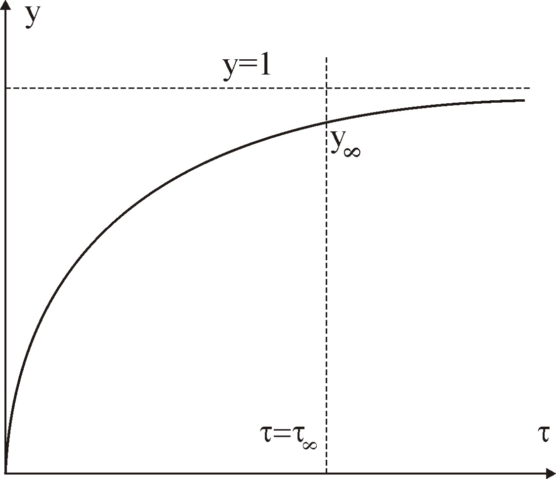
Figure 3: Qualitative form of function’s $y(\tau)$ graph.

6 Exact model of transition from the ultrarelativistic stage to the inflationary one

Let us consider a simple model of matter consisting of 2 components (see for details [27, 28, 29]) – minimally coupled massive scalar field (cosmological member) with a state equation:

$$p_{s}=-\varepsilon_{s},$$ (134)

and the ultrarelativistic plasma with the state equation (78). Then summary barotropic factor and invariant acceleration can be written in form:

$$\varkappa(t)=\frac{1}{3}\frac{1-3\delta}{1+\delta};\quad\Omega(t)=-\frac{1-\delta}{1+\delta},$$ (135)

where

$$\delta=\delta(t)=\frac{\varepsilon_{s}}{\varepsilon_{p}}.$$ (136)

Thus at $\delta={\rm Const}$ formulas(74) can be written in the following convenient form [28, 29]:

$$a=a_{1}t^{(1+\delta)/2};\;\varepsilon=\frac{3}{32\pi}\frac{(1+\delta)^{2}}{t^{2}},\quad\Omega<1.$$ (137)

Energy conservation laws (76) – (77) take form:

$$\varepsilon_{s}={\rm Const}=\frac{3\Lambda^{2}}{8\pi};$$ (138)

$$\varepsilon_{p}a^{4}\equiv\tilde{\varepsilon}_{p}={\rm Const}\simeq\frac{3}{32\pi}.$$ (139)

Substituting (157)-(158 )into the equation (68) and integrating it, we obtain:

$$\!\!a(t)=\frac{1}{\sqrt{2}}\left[\left(t_{0}+\sqrt{t^{2}_{0}+b^{2}}\right){\rm e}^{(t-t_{0})/2\Lambda}-\frac{b^{2}}{t_{0}+\sqrt{t^{2}_{0}+b^{2}}}{\rm e}^{-(t-t_{0})/2\Lambda}\right]^{\frac{1}{2}},$$ (140)

where:

$$b^{2}=\frac{3}{32\pi\Lambda^{2}}.$$ (141)

Hence we have, in particular, for the scale factor at $t_{0}=0$:

$$a(t)=\frac{1}{\Lambda}\sqrt{\frac{3}{32\pi}{\rm sh}\frac{t}{2\Lambda}}$$ (142)

Calculating according to (136), (157), (158) and (159) the relation $\delta$, we find:

$$\delta(t)=\left(\frac{3}{16\pi\Lambda}\ {\rm sh}\frac{t}{2\Lambda}\right)^{2}.$$ (143)

Next, according to(136) it is possible to calculate an effective barotropic factor and an invariant acceleration (see Figure 4).

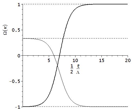
Figure 4: Evolution of the effective barotropic factor $\kappa(t)$ (thin line) and invariant acceleration $\Omega(t)$ (heavy line) relative to the exact solution (159) at $\Lambda=1$. Asymptotes $-1;\;1/3;\;1$ are denoted by the dotted lines.

Following figure shows that by means of parameter $\Xi$ it is easy to control the time of transition to the inflationary acceleration regime $\kappa\to-1$. Let us recall that cosmological time $t$ is measured in Planck units.

Thus according to(103) we can determine the new dimensionless time variable $\tau$:

$$\tau=\frac{2\Lambda\langle\xi\rangle}{\langle\tilde{p}\rangle_{0}}{\rm F}(\varphi,1/\sqrt{2}),$$ (144)

where:

$$\varphi=\arccos\frac{1-{\rm sh}\;t/2\Lambda}{1+{\rm sh}\;t/2\Lambda};$$ (145)

${\rm F}(\varphi,k)$ is an elliptic integral of the first type (see e.g.:

$${\rm F}(\varphi,k)=\int\limits_{0}^{\varphi}\frac{d\alpha}{\sqrt{1-k^{2}\sin^{2}\alpha}};\quad(k^{2}<1).$$ (146)

Thus:

$$\frac{d\tau}{dt}=\frac{1}{2\Lambda}\frac{1}{{\rm sh}\;\varphi}\frac{{\rm ch}\;\varphi}{1+{\rm sh}\;\varphi}>0;\quad\tau\in[0,\tau_{\infty}),$$ (147)

where

$$\tau_{\infty}=\lim\limits_{t\to+\infty}\tau(t)=\frac{2\Lambda\langle\xi\rangle}{\langle\tilde{p}\rangle_{0}}{\rm F}(1,1/\sqrt{2}),$$ (148)

$F(1,1/\sqrt{2}\approx 1.083216773$.

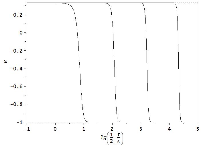
Figure 5: The evolution of the barotrope effective coefficient $\kappa(t)$ relative to the exact solution (159) subject to the cosmological constant $\Lambda$ left to right: $\Lambda=1$, $\Lambda=10$, $\Lambda=100$, $\Lambda=1000$.

7 The numerical model of LTE restoration in the accelerating Universe

7.1 The model of the initial non-equilibrium distribution

Thus, as it has been mentioned above, the mathematical model of LTE restoration process in cosmological plasma is reduced to two parametric equations

$$\int\limits_{0}^{Z}\frac{du}{\sqrt{1-(1-\sigma_{0})\Phi(u)}}=\tau.$$ (149)

$$y=[1-(1-\sigma_{0})\Phi(Z)]^{1/4},$$ (150)

which at given function $\Phi(Z)$ define the relations of form:

$$\tau=\tau(Z);$$ (151)

$$y=y(Z),$$ (152)

solving which we can determine function $y(\tau)$ and thereby formally solve stated problem completely. Thus, the final solution of the task is found in quadratures specifying the initial distribution of non-equilibrium particles $\Delta f_{0}(p)$ and following definition of the integral function $\Phi(Z)$:

$$\Phi(Z)\equiv{\displaystyle\frac{\sum\limits_{a}(2S+1)\int\limits_{0}^{\infty}d\rho\rho^{3}\Delta f^{0}_{a}(\rho){\rm e}^{\displaystyle-\frac{Z(\tau)}{\rho}}}{\sum\limits_{a}(2S+1)\int\limits_{0}^{\infty}d\rho\rho^{3}\Delta f^{0}_{a}(\rho)}}.$$ (153)

Let us note that formally parametric equations (149) and (150), as well as function’s $\Phi(Z)$ definition, do not differ from the similar, obtained earlier by the Author in articles [5], [24]. The main new statement is brought by the acceleration of the Universe and consists in the relation $\tau(t)$ (103).

In order to construct a numerical model let us consider the initial distribution of white noise type:

$$\Delta f_{0}(\rho)=\frac{A}{\rho^{3}}\chi(\rho_{0}-\rho),$$ (154)

where $A$ is a normalization constan, $\rho_{0}>1$ is a dimensionless parameter, $\chi(x)$ is a Heaviside step function, so that the conformal energy density with respect to this distribution is equal to:

$$\tilde{\varepsilon}^{0}_{ne}=\frac{\langle\tilde{p}\rangle_{0}^{4}A\rho_{0}}{32\pi^{5}}.$$ (155)

Calculating function $\Phi(Z)$ relative to distribution (154), we find:

$$\Phi(Z)=e^{-x}-x{\rm Ei}(x);\quad x\equiv\frac{Z}{\rho_{0}},$$ (156)

where ${\rm Ei}(x)$ is an integral exponential function

$${\rm Ei}(x)=\int\limits_{-1}^{\infty}\frac{e^{-tx}}{t}dt.$$

7.2 The results of numerical integration

Thus, the problem is reduced to the numerical integration of the system of equations (103), (149), (150). Below the certain integration results are represented. Further according to (76)–(78)

$$\varepsilon_{s}={\rm Const}=\frac{3\Lambda^{2}}{8\pi};$$ (157)

$$\varepsilon_{p}a^{4}\equiv\tilde{\varepsilon}_{p}={\rm Const}\simeq\frac{3}{32\pi}.$$ (158)

and (159)

$$a(t)=\frac{1}{\Lambda}\sqrt{\frac{3}{32\pi}{\rm sh}\frac{t}{2\Lambda}}$$ (159)

it may be convenient to introduce a time cosmological constant

$$t_{0}\equiv 4\Lambda.$$ (160)

In article [30] there was described Author’s program designed with Maple v15 and intended for the numerical simulation of the presented above mathematical model of thermodynamic equilibrium’s restoration in the Universe. Model included transition to the acceleration stage. Below we describe the results of numerical modeling in-detail and carry out the analysis.

On Figure 6 the results of numerical integration for the definition of the parameter $\tau_{\infty}$ are shown.

Figure 6: Dependency of the dimensionless time variable’s $\langle\tilde{p}\rangle_{0}\tau$ common logarithm on the cosmological time $t$. Bottom-up: $t_{0}=1$; $10$; $10^{2}$; $10^{3}$; $10^{4}$; $10^{5}$. It is introduced everywhere $N_{0}=100$; $N=10$.

In particular, the integration of the relation (103) confirmed insensitivity of value $\tau_{\infty}$ from the number of parameters and, practically, confirmed the estimation formula (103) [27]

$$\tau_{\infty}=\lim\limits_{t\to+\infty}\tau(t)=\frac{2\Lambda\langle\xi\rangle}{\langle\tilde{p}\rangle_{0}}{\rm F}(1,1/\sqrt{2}),$$ (161)

which did not account the details of the logarithmical dependency of the parameter $\langle\xi\rangle$ on time. On Figure 7 the results of this value’s numerical integration are shown.

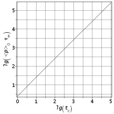
Figure 7: Dependency of the dimensionless time parameter $\tau_{\infty}\langle\tilde{p}\rangle_{0}$ on the time cosmological constant $t_{0}\equiv t_{c}$ (160); everywhere is $t_{c}=1$; $N_{0}=100$; $N=10$, $\langle\tilde{p}\rangle_{0}$; $\sigma_{0}$ — bottom-up: 0.01; 0.1; 0.2; 0.5.

These results are well described by formula

$$\tau_{\infty}\approx\frac{2.57t_{0}}{\langle\tilde{p}\rangle_{0}}.$$ (162)

On Figure 8 the dependency of the variable Z(t) at different values of time cosmological constant is shown.

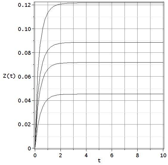
Figure 8: Dependency of the dimensionless function $Z(t)$ on time; it is everywhere $t_{c}=1$; $N_{0}=100$; $N=10$, $\langle\tilde{p}\rangle_{0}=10$; $\sigma_{0}$ — bottom up: 0.01; 0.1; 0.2; 0.5.

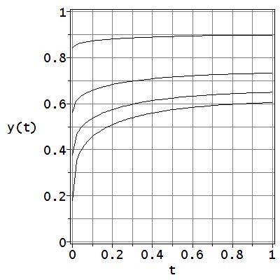
Figure 9: Dependency of the relative temperature $y(t)$ on time; it is everywhere $t_{c}=1$; $N_{0}=100$; $N=10$, $\langle\tilde{p}\rangle_{0}=10$; $\sigma_{0}$ — bottom up: 0.01; 0.1; 0.2; 0.5.

As it is follows from the results represented on this figure, function’s $Z(t)$ value also has a limit value at $t\to\infty$:

$$\lim\limits_{t\to\infty}Z_{\infty}<\infty.$$ (163)

According to (106)

$$\Delta f_{a}(\tau,\rho)=\Delta f^{0}_{a}(\rho)\cdot{\rm e}^{\displaystyle-\frac{Z(\tau)}{\rho}},$$ (164)

this means that at $t\to\infty$ superthermal particles’ distribution is “frozen”:

$$\Delta f_{a}(\tau_{\infty},\rho)=\Delta f^{0}_{a}(\rho)\cdot{\rm e}^{-\frac{Z_{\infty}}{\rho}}.$$ (165)

Thus, in modern Universe there can remain the “tail” of non-equilibrium particles of extra-high energies:

$$E\gtrsim E_{\infty}=Z_{\infty}\langle\tilde{p}\rangle_{0}.$$ (166)

On Figure 10–11 the results of numerical integration for the relative temperature $y(t)=T(t)/T_{0}(t)\leq 1$ are shown. According to the meaning of that value the dimensionless parameter:

$$e_{\infty}=1-\sigma_{\infty}=1-y^{4}_{\infty}>0$$ (167)

is a relative part of cosmological plasma’s energy concluded in this non-equilibrium “tail” of distribution.

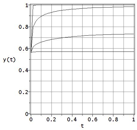
Figure 10: Dependency of the relative temperature $y(t)$ on time; it is everywhere $\sigma_{0}=0.1$; $N_{0}=100$; $N=10$, $\langle\tilde{p}\rangle_{0}=10$; $t_{c}$ — bottom-up: 0.1; 1; 10; 100.

Figure 11: Dependency of the relative temperature $y(t)$ on time; it is everywhere $\sigma_{0}=0.01$; $N_{0}=100$; $N=10$, $\langle\tilde{p}\rangle_{0}=1000$; $t_{0}$ — bottom-up: 1; 10; 100; 1000.

7.3 Asymptotic values of parametres of nonequilibrium distribution at an inflationary stage

For the observation in present age of the Universe the knowledge of possible limiting values of parametres of nonequilibrium distribution of particles is important. Such probable observable parametres are the relative temperature $y_{\infty}$, the relative part of energy concluded in the nonequilibrium tail of distribution, and also the form of this distribution. On Figure 12, 13, 14, 15, 16, 17 the calculated values of the first two parametres are presented.

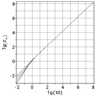
Figure 12: Dependency of the dimensionless function $Z_{\infty}$ on cosmological constant $t_{0}$; it is everywhere $\langle\tilde{p}\rangle_{0}=100$; $N_{0}=100$; $N=10$; $\sigma_{0}$ — bottom-up: 0.001; 0.01; 0.1; 0.5.

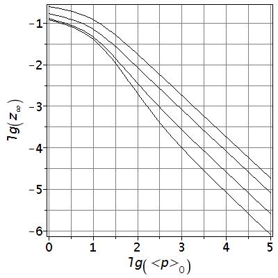
Figure 13: Dependency of the dimensionless function $Z_{\infty}$ on parameter $\langle\tilde{p}\rangle_{0}$; it is everywhere $t_{0}=1$; $N_{0}=100$; $N=10$; $\sigma_{0}$ — bottom-up: 0.001; 0.01; 0.1; 0.5.

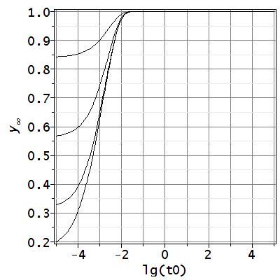
Figure 14: Dependency of the relative temperature $y_{\infty}$ on cosmological constant $t_{0}$; it is everywhere $t_{0}=1$; $N_{0}=100$; $N=10$; $\sigma_{0}$ — bottom-up: 0.001; 0.01; 0.1; 0.5.

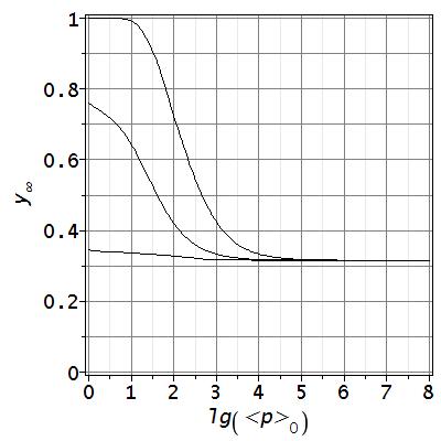
Figure 15: of the relative temperature $y_{\infty}$ on parameter $\langle\tilde{p}\rangle_{0}$; it is everywhere $\sigma_{0}=0.1$; $N_{0}=100$; $N=10$; $t_{0}$ — bottom-up: 0.1; 1; 10.

7.4 Analysis of numerical simulation

From these results it follows, that starting from values of parameter $\langle\tilde{p}\rangle_{0}$ of the order of 10-100, the survival of considerable number of nonequilibrium relic particles at modern stage of Universe evolution is possible. It is the striking fact as we recall that according to the results of the Author’s early papers, considering standard cosmological scenario which excludes inflationary stage, at the modern stage of expansion it is only relic particles with energy of an order $10^{12}$Gev and above which can survive. At presence of a modern inflationary stage nonequilibrium relic particles with energy of an order of 1 Kev can survive!

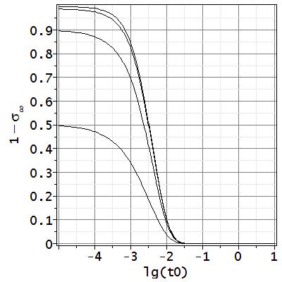
Figure 16: Dependence of a relative part of energy of nonequilibrium particles, $1-\sigma_{\infty}$, on cosmological constant $t_{0}$; it is everywhere $\langle\tilde{p}\rangle_{0}=1000$; $N_{0}=100$; $N=10$, $\sigma_{0}$ — top-down: 0.001; 0.01; 0.1; 0.5.

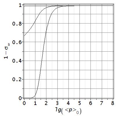
Figure 17: Dependence of a relative part of energy of nonequilibrium particles, $1-\sigma_{\infty}$, on cosmological constant $t_{0}$; it is everywhere $\sigma_{0}=0.01$; $N_{0}=100$; $N=10$, $\langle\tilde{p}\rangle_{0}=1000$; $t_{0}$ — top-down: 0.1; 1; 10.

On Figure 19 the evolution of distribution of density of energy of nonequilibrium particles in the assumption of their initial distribution in form

$$\left(\frac{d\varepsilon}{d\rho}\right)_{0}=A\frac{\chi(\rho_{0}-\rho)}{(1+\rho/\langle\tilde{p}\rangle_{0})^{3}}$$ (168)

is represented.

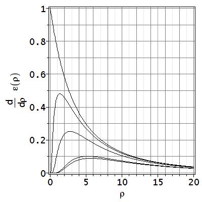
Figure 18: Evolution of density of distribution of energy; it is everywhere $\sigma_{0}=0.5$; $N_{0}=100$; $N=10$, $\langle\tilde{p}\rangle_{0}=10$, $t_{0}=1$; from top to down: t= 0.0001; 0.01; 0.1; 1; 10; 100. Lines at t=10 and t=100 are coincide.

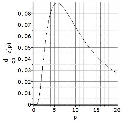
Figure 19: Fixing of nonequilibrium function of distribution at $t=\infty$. $\sigma_{0}=0.5$; $N_{0}=100$; $N=10$, $\langle\tilde{p}\rangle_{0}=10$, $t_{0}=1$.

Calculating a maximum of distribution of density of energy from a relationship (106), we will find:

$$\rho_{\infty}^{max}=\sqrt{Z_{\infty}\langle\tilde{p}\rangle_{0}}.$$ (169)

On Figure 20 the dependency of the maximum of energy spectrum of nonequilibrium particles on cosmological constant $t_{0}$ is presented. From this figure it is apparent, that at not very great values of the cosmological constant, the maximum of energy spectrum of nonequilibrium particles is in the field of quite low energies, that, of course, means their detection is possible in space conditions.

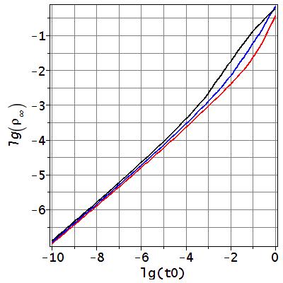
Figure 20: Dependence of relativity limiting energy of a maximum $\lg\rho_{\infty}$ of distribution on a cosmological constant at $\sigma_{0}=0.01$, $N_{0}=100$; $N=10$. Red line – $\langle\tilde{p}\rangle_{0}=1$, blue line – $\langle\tilde{p}\rangle_{0}=10$, black line – $\langle\tilde{p}\rangle_{0}=100$.

Let’s notice, that value of dimensionless energy $\rho$ actually means, that in present period the particle has energy which $\rho\langle\tilde{p}\rangle_{0}$ times bigger than temperatures of relic radiation. Thus, in present period we can observe truly relic particles with energies of order of 1 Kev and more in a maximum of the distribution. Speaking about ”truly relic particles”, we mean the particles which have survived from the moment of the Universe birth, unlike relic photons or neutrino, which were formed at the radiationally-dominated stage of the Universe. Detection of truly relic particles in cosmic space would allow to receive the information about the moment of the Universe birth, and also about elementary particles interaction specifics at extra-high energies which never would be attainable by mankind.

In the next article we will consider the process of restoration of thermodynamic equilibrium in the Universe with real parameters of the cosmological constant $\Lambda$.

References

References

- [1] Steven Weinberg. Cosmology, Oxford University Press, 2008.
- [2] H.M. Pilkuhn. Relativistic Particle Physics, Springer-Verlag, New York Inc, 1979.
- [3] Yu.G. Ignat’ev, J. Sov. Phys. (Izv. Vuzov). 25 No 4, 92 (1982)
- [4] Yu.G. Ignat’ev, in: “Actual theoretical and experimantal problems of relativity theory and gravitation”, Report of Soviet conference, Moscow, 1984 (in Russian).
- [5] Yu.G. Ignat’ev, J. Sov. Phys. (Izv. Vuzov). 29, No 2, 19 (1986).
- [6] L.B. Okun, Leptons and quarks, North-Holland, Amsterdamm Oxford New-York Tokyo, 1981.
- [7] L.D. Landau, J.Sov.Phys. (JETP), 10, 718 (1940).
- [8] M. Froissart, Phys. Rev., 123, 1053 (1961)
- [9] A. Martin, Phys. Rev., 129, 1432 (1963)
- [10] A. Martin, Nuovo. Cim., 142, 930 (1966)
- [11] Y.S. Jin, A. Martin, Phys. Rev.B 135, 1369 (1964)
- [12] M. Sugawara, Phys. Rev. Lett., 14, 336 (1965)
- [13] R.I. Eden, High Energy Collisions of Elementary Particles, Cambridge At the University Press, 1967
- [14] J.D. Bjorken, E.A. Paschos, Phys. Rev., 185, 1975 (1969)
- [15] R.P. Feyman, Phys. Rev. Lett., 23, 1415 (1969)
- [16] N. Cabibo, G. Parivisi, M. Tesla, Lett. Nuovo. Cimento,35, 4. (1970)
- [17] L.P. Gritchuk, J. Sov. Phys. (JETF), 67, 825 (1974).
- [18] Yu.G.Ignatyev, Gravitation & Cosmology Vol.13 (2007), No. 1 (49), pp. 1-14.
- [19] Yu.G. Ignat’ev, J. Sov. Phys. (Izv. Vuzov). 23 No 8, 42 (1980).
- [20] Yu.G. Ignat’ev, J. Sov. Phys. (Izv. Vuzov). 23 No 9, 27 (1980).
- [21] Yu.G.Ignatyev, in: Problems of Gravitation Theory and Elementary Particles, Moskow, Atomizdat, No 11, 113 (1980).
- [22] Yu.G. Ignat’ev, J. Sov. Phys. (Izv. Vuzov). 26, No 8, 19 (1983).
- [23] Yu.G. Ignat’ev, J. Sov. Phys. (Izv. Vuzov). 26 No 12 9 (1983)
- [24] Yu.G.Ignatyev, D.Yu.Ignatyev, Gravitation & Cosmology Vol.13 (2007), No. 2 (50), pp. 101-113
- [25] L.D. Landau, E.M. Lifshitz. Statistical Physics. Vol. 5 (3rd ed.). Pergamon Press. Oxford New York Toronto Sydney Paris Frankfurt, 1980.
- [26] L.D. Landau, E.M. Lifshitz. The Classical Theory of Fields. Pergamon Press. Oxford New York Toronto Sydney Paris Frankfurt, 1971
- [27] Yu. G. Ignat’ev, Russian Physics Journal, Vol. 56, No. 6, November, 2013. - p. 693-706 DOI: 10.1007/s11182-013-0087-4
- [28] Yurii Ignatyev, arXiv:1306.3633v1 [gr-qc] 13 June 2013.
- [29] Yu.G. Ignatyev, Grav. and Cosmol., to be publish in vol. 19, No 4, 2013.
- [30] Yu. G. Ignat’ev, Russian Physics Journal, to be publish in Vol. 57, No. 1, Jenuvary, 2014; Yu.G. Ignatyev, arxiv.org/pdf/1310.2183.pdf [gr-qc] 8 October 2013.